Abstract
Annuity insurance is a crucial financial tool for mitigating risks associated with aging, yet it has not gained significant traction in China’s insurance market, especially amid the challenges posed by an aging population. This study develops a discrete-time multi-period life-cycle model to analyze optimal annuity purchases for China’s middle-aged population under disability risk and explores in depth the impact and underlying mechanisms of disability risk on their annuity insurance purchase decisions. Disability is endogenized via two channels: financial-constraint effects (medical costs and pre-retirement income loss) and stochastic health state transitions with recovery and mortality. Using data from China Health and Retirement Longitudinal Study (2018–2020) to estimate age- and gender-specific transition matrices and data from China Household Finance Survey (2019) to link income with initial assets, we solve the model by the endogenous grid method and simulate actuarially fair annuities. The findings reveal substantial under-demand for annuities among China’s middle-aged population. Under inflation, the modest yield premium of annuities over inflation significantly depresses purchases by middle- and low-wealth households, while high-wealth individuals are jointly constrained by rapidly rising health expenditures and inadequate annuity returns. Notably, behavioral patterns could shift fundamentally under a hypothetical zero-inflation scenario.
MSC:
91G05
1. Introduction
China is currently facing the complex issue of population aging. Annuity insurance, a significant financial instrument tailored to mitigate individual risks associated with aging, can effectively mitigate the financial burden on the elderly by ensuring a steady income. Despite its potential benefits, annuity insurance remains underutilized in the current insurance market, with a generally low market penetration rate and limited demand. The gap between theoretical predictions and real-world participation is known as the “annuity puzzle”. Based on expected utility theory, Yaari demonstrated that, under actuarially fair pricing and in the absence of bequest motives, rational individuals should allocate all their wealth to annuities to maximize their lifetime utility [1]. Nevertheless, real-world data show that annuity participation rates are insufficient. For example, in the United States, only 6% of 401K plan participants choose to annuitize their assets [2], and in the United Kingdom, the proportion of households voluntarily allocating to annuities is only 5.9% [3]. In China, premium income from retirement annuity insurance accounted for only 2% of the total premium income of life insurance companies in 2022 (source: http://m.ce.cn/cj/202301/30/t20230130_38364990.shtml (accessed on 30 January 2023)).
The essence of the annuity puzzle lies in the gap between theoretical predictions and actual behavior. The life-cycle and dynamic programming framework provides a unified perspective for studying household decisions on consumption, saving, and insurance under uncertainty. Since Modigliani and Brumberg proposed the life-cycle hypothesis, the intertemporal allocation of resources across one’s lifetime has become the starting point for understanding insurance and wealth dynamics [4]. Subsequently, Samuelson and Merton embedded consumption–investment choices within dynamic (stochastic) programming and continuous-time optimization, laying the theoretical and methodological foundation for joint optimization in multi-period state-dependent environments with constraints and incomplete markets [5,6,7]. Gourinchas and Parker’s structural estimation further characterizes the systematic variation in risk exposure and consumption–saving paths across different life stages [8].
The life-cycle–dynamic programming framework also offers multiple quantifiable explanatory mechanisms for the annuity puzzle. Background risks such as income and medical shocks induce households to dynamically trade off between “self-insurance” (precautionary saving, buffer-stock wealth) and “market insurance” (life, health, and annuities). Hubbard et al. use a stochastic life-cycle model to conclude that means-tested welfare programs disincentivize saving, leading to the prevalence of low-wealth households [9]. Market and institutional frictions (loadings, fees, adverse selection, and supply-side constraints) reduce the monetary worth of annuities [10], weakening their appeal. When facing income and medical risks and borrowing constraints, households tend to maintain liquidity buffers and self-insure [11], thereby reducing reliance on rigid annuitization. Heterogeneity in family structure, bequest motives, and longevity or health expectations further undermines the universality of full annuitization [12]. Reichling and Smetters (2015) and Peijnenburg et al. (2017) pointed out that high medical costs reduce the present value of annuities, and when liquidity is needed to cope with health shocks in early retirement, it may be optimal to shorten annuities [13,14]. Chen and Fan showed that health risks significantly suppress annuity demand among elderly individuals with moderate wealth [15]. Yogo developed a life-cycle model with stochastic health depreciation, in which retirees make decisions regarding consumption, health expenditures, and the allocation of wealth across assets [16]. This model explains the characteristics of asset allocation and health expenditures across different health statuses and age groups. To evaluate why the uptake of Long-term Care Insurance (LTCI) and annuities is so low, Timo and Frederik provide an overview of all factors impacting LTCI and annuity purchase decisions [17].
Across the above studies, it is consistently highlighted that, in the causes of the annuity puzzle, health risks play a crucial role. Although the average life expectancy of residents in China has increased, the healthy life expectancy has not extended at the same pace [18]. Individuals may prioritize saving funds to cope with potential high medical expenses, income loss, and care costs due to disability, rather than purchasing annuities. In other words, health risks increase financial uncertainty.
However, some studies have also pointed out that health risks can increase the demand for annuities. Pang and Warshawsky argued that after incorporating health risks, annuities become more attractive because they better hedge mortality risk and are safer than stocks, thus increasing demand [19]. Ai et al. found that when the average duration of disability in old age is longer, the demand for annuities rises [20].
Moreover, there are studies on other interaction effects. Koijen et al., Hambel et al., Ameriks et al., Hambel, Chen et al., and Chen et al. examined the optimal allocation and interaction effects between annuities and other types of insurance (such as life insurance, long-term care insurance, and critical illness insurance) under health risks [21,22,23,24,25,26].
Despite advancements in current research, several limitations persist. Firstly, the literature predominantly overlooks specific age demographics, primarily focusing on the elderly while neglecting to delve deeply into the distinct health risks and financial requirements of China’s middle-aged “baby boomer” cohort as they approach old age. Secondly, the analysis of causal mechanisms remains superficial, with some studies incorporating elements such as disability health expenses and inflation projections into life-cycle models without thoroughly exploring their influence on individual decision-making processes. Lastly, the refinement of model parameters remains inadequate, as most multi-period life-cycle models merely consider health state transitions and associated costs in assessing disability health risks, disregarding potential income loss during periods of disability. Moreover, income is typically treated as a constant, with minimal consideration given to variations in initial assets.
To address the aforementioned limitations and to better reveal the mechanisms through which health risk affects annuity purchase decisions, this study introduces the following innovations and contributions:
This study targets the middle-aged population amid China’s rapid aging demographic. The forthcoming waves of the “baby boomer” cohort, specifically those born between 1962–1975 and 1981–1991, are anticipated to reach old age en masse by 2027 and 2046, respectively [27]. Unlike the elderly with high health expenses and limited asset appreciation time or the youth with a lesser awareness of longevity risks, the current middle-aged “baby boomer” demographic possesses a solid economic foundation. They are currently grappling with the dual imperatives of retirement planning and healthcare security. Consequently, this group, being emblematic and pivotal in annuity insurance acquisition and retirement security decision-making, warrants focused investigation [28]. By concentrating on this demographic, this study aims to scrutinize the annuity insurance demand and decision-making processes, shedding light on their behavioral traits. Such insights hold significant practical implications for enhancing pension financial systems and addressing the challenges posed by population aging.
The bottleneck identified in this study is how a middle-aged person’s financial vulnerability, under the impact of health risk, systematically alters the mechanism of optimal annuity decision-making. Our model innovation is designed to more precisely capture the abovementioned financial constraint effects. This allows us to move beyond simplistic explanations based on “psychological reluctance” and reveal the root causes of the bottleneck at the micro-mechanism level of decision-making.
In terms of model innovation, a “log–log linear income–asset regression model” is incorporated into the multi-period life-cycle framework. By introducing dynamic income and asset structures that vary with health status and life-cycle stage, the model setting better reflects real-world conditions. Health risk is focused specifically on disability risk, with key model assumptions including health state transition probabilities, inflation expectations, and disability costs, while also incorporating income loss due to disability. Through controlled variables, this study separately examines the impact of these factors on the annuity insurance decisions of the middle-aged population. Our model more accurately reflects the financial vulnerability and changes in insurance demand faced by the middle-aged group when encountering health shocks, thereby enhancing the scientific rigor of the analysis and the relevance of the policy recommendations.
2. Construction and Solution of a Multi-Period Life-Cycle Model Based on Disability Risk
2.1. Theoretical Preparation: Dynamic Programming Algorithm
Dynamic programming was proposed by Bellman to solve optimization problems in multi-stage decision-making processes [29]. Its core idea is to decompose complex problems into multiple sequential decision stages (i.e., ). At each stage, based on the current state , a decision is made, which drives the state transition through either of the following:
- (1)
- Deterministic transition: or
- (2)
- Stochastically ,
where denotes the state transition probability measure. Within this framework, the sequence of decisions can be optimized according to an objective function, such as the total lifetime utility
where represents the instantaneous utility function, and denotes the expectation accounting for stochastic transitions. is the discount factor. The effectiveness of this algorithm requires two key properties:
- (1)
- Optimal substructure: any sub-policy of an overall optimal policy must itself be optimal for its corresponding starting state.
- (2)
- Markov property: the evolution of future states depends only on the current state and decision , and is independent of the historical path.
2.2. Model Design
In this study, the annuity purchase decision is modeled as a discrete-time stochastic multistage decision problem, in which the state variables include assets, health status, and income, and the transition of health status is stochastic. Within this framework, the dynamic programming approach can effectively characterize and solve an individual’s optimal decision path under uncertainty at different stages.
An individual lifetime expected utility maximization model was constructed. Utility is derived from consumption and bequest , subject to three constraints.
- (1)
- Consumption lower bound (the minimum subsistence level);
- (2)
- Consumption upper boundwhere is the minimum subsistence level at time , is the labor income at time , represents the assets at time , and is the disability cost at time . If the individual becomes disabled before retirement, then until the person recovers or retires, reflecting the loss of labor income due to disability;
- (3)
- Asset accumulation equation
The health status evolves stochastically according to the transition probability . In particular, 4 represents death, which is an absorbing state, and does not transition to any other health status.
The core Bellman equation is as follows:
If ,
subject to the budget constraint
where
If ,
where is the subjective discount factor. is the maximum expected lifetime utility starting from time , health status , and assets , under optimal decisions at present and in the future.
The analysis concerns a stochastic system. Health status and assets represent the state variables, and serves as the control variable.
2.3. Model Solution
The above model is numerically solved using the endogenous grid method (EGM) proposed by Carroll, as follows [30].
- (1)
- Parameter Setting and Initialization
Suppose the terminal period of the life cycle is , with a subjective discount factor and an asset grid .
The value function is initialized at the terminal period .
If (alive), , subject to the constraints,
If (dead), .
- (2)
- Backward induction (from to )
For each period and health status (alive), the following steps are performed.
Step 1: Construct the expected value function for the next period.
Define the asset grid points for the next period , and compute the interpolation function for the derivative of the expected value function.
For (death), the derivative is . For (alive), the derivative is interpolated from the discrete grid values.
Step 2: Compute the optimal consumption using the first-order condition.
For each , solve the first-order condition
to obtain the optimal consumption of
Thus, the current-period asset is calculated as follows:
Step 3: Handle the constraint conditions.
Consumption lower bound constraint (): if , enforce , and recalculate the asset ; non-negativity constraint (): only include in the grid ; the consumption upper bound constraint is automatically satisfied, because is guaranteed by the budget constraint.
Step 4: Calculate the value function.
For each , the value function is calculated as follows: .
Step 5: Construct the current-period value function.
Collect the set of points , sort by , and build continuous functions and through interpolation (such as linear interpolation).
- (3)
- Handle the death state.
If , direct assignment
- (4)
- Forward simulation.
Starting from the initial state , the optimal consumption function and the health state transition probability are used to simulate the entire life-cycle path.
2.4. The Core of the Multi-Period Life-Cycle Model Based on Disability Risk
2.4.1. Optimal Annuity Purchase Decision
The annuity insurance product considered in this study is a one-time premium payment at age :
where is the purchase proportion, and represents the initial assets. From the retirement period onward, the policyholder receives a survival benefit of each period (assuming that each 1 unit of premium currently provides an annual annuity payment of beginning at retirement).
The optimal proportion is determined via a discrete grid search: in the interval [0,1], choose an equally spaced set of points . For each , the model parameters are adjusted as follows: initial assets are adjusted to , and after retirement (), income is corrected as . A forward simulation is then performed to calculate the expected utility . The that maximizes is taken as the optimal annuity purchase proportion, and the optimal purchase amount is .
2.4.2. The Endogenous Characterization Mechanism of Disability Risk
The model endogenizes disability risk through a dual mechanism, which in turn shapes annuity purchase decisions.
- (1)
- Financial constraint effect: The disabled state triggers disability-related health costs (which directly deplete current assets ) and potential income loss (caused by disability before retirement), both of which jointly reduce the disposable resources available for consumption and annuity premium payments.
- (2)
- State transition randomness: The health state evolves stochastically according to an age-dependent transition probability matrix
The probability of health deterioration (transition to the disabled state) directly affects individuals’ expectations regarding future high medical expenses and the risk of income interruption, prompting them to weigh the potential liquidity risk against the risk of premium loss due to premature death when purchasing annuities (which provide longevity risk protection). The probability of death is associated with the strength of bequest motives and demand for annuity survival benefits.
3. Empirical Analysis of Optimal Annuity Insurance Decisions for the Middle-Aged Population
3.1. Definition of Core Concepts
The definitions of the key concepts in this study are as follows:
- (1)
- Middle-aged and elderly population. Based on the World Health Organization’s age classification standards and China’s gradually delayed retirement policy (to be implemented from 2025), individuals aged above 45 are defined as entering middle age, with above 65 as the starting point for old age and retirement.
- (2)
- Annuity insurance. This specifically refers to individual annuity insurance products within the personal pension security system.
- (3)
- Health status. According to the Activity of Daily Living Scale (ADL), individual health status is divided into four discrete levels: healthy (no impairment in either the Physical Self-Maintenance Scale (PSMS) or Instrumental Activities of Daily Living (IADL), mildly disabled (1–2 impairments in only one of the two abilities), severely disabled (surviving but not falling into the above two categories), and deceased.
3.2. Data Resource
3.2.1. China Health and Retirement Longitudinal Study (CHARLS)
This study used CHARLS as the primary data source. CHARLS adopts internationally standardized questionnaires and systematically collects individual health data through a multidimensional indicator system covering dimensions such as physiological indicators, prevalence of chronic diseases, activities of daily living (ADL), cognitive function, mental health, and utilization of medical services. This enables effective classification of health status based on the Physical Self-Maintenance Scale (PSMS) and Instrumental Activities of Daily Living Scale (IADL).
CHARLS has completed five waves of nationwide longitudinal surveys from 2011 to 2020, with panel response rates exceeding 80% for each wave from 2013 to 2020. This ensures strong timeliness and validity for longitudinal analysis, providing high-quality data to support the estimation of health state transition probabilities among the middle-aged population. According to the definition of the middle-aged group in this study (starting from the end of age 45), the study sample is highly consistent with the CHARLS sample of individuals aged 45 and above. The age distribution of the data shows that the sample is mainly concentrated in the 46–70 age range and is approximately normally distributed, effectively avoiding age discontinuity issues and ensuring good representativeness of the sample.
3.2.2. China Household Finance Survey (CHFS)
This study uses data from the 2019 CHFS. The project adopts a probability proportional to size (PPS) sampling method, covering 355 districts and counties across 29 provinces nationwide, and has collected micro-level financial data from 40,011 households, making it the largest non-official household asset survey in China. The data provide detailed records of household social security, commercial insurance, and subjective attitudes, providing a reliable basis for the financial parameters used in this study.
According to the CHFS 2019 data, approximately 90% of individuals aged 46 years have assets of CNY 750,000 or less. Our subsequent analysis of annuity purchase decisions sets the initial asset upper limit at CNY 750,000.
3.2.3. Data Integration and Application
- (1)
- Health state transition probabilities: based on CHARLS panel data from 2018 to 2020, two-year health state transition probabilities were calculated by age group and then converted into five-year probability matrices, which serve as the core parameters of the life-cycle model.
- (2)
- Income–asset relationship modeling: using CHFS 2019 data, a log–linear regression model of income and assets for individuals aged 46 years is constructed to estimate the income trajectories of individuals with different initial asset levels.
The selection of the 2019 CHFS data was motivated by the complementary strengths of the datasets. While CHARLS excels in health and retirement details, it lacks comprehensive data on household assets and income. Conversely, CHFS provides detailed household balance sheets and income flows, crucial for accurately fitting our income–asset regression model. Despite being separate, both are high-quality nationally representative surveys of the middle-aged population. By leveraging CHARLS for health transitions and CHFS for financial modeling, we optimize the parameter estimation methodologically, enhancing the accuracy without introducing systematic bias.
3.3. Income–Asset Model
3.3.1. Design of the Log–Log Linear Income–Asset Regression Model
The existing literature typically sets income in each period as a fixed value (such as the national average income) and only examines the impact of asset variation on the proportion of annuity purchases [15,31].
However, this approach deviates from real-world economic logic: among individuals of the same age group, where assets and income are positively correlated, and those with higher assets generally have higher income. According to the descriptive statistics of 2019 CHFS (see Appendix A, Table A1 for details), there may be a positive correlation between income and assets. However, since both variables exhibit highly uneven distributions and large standard deviations (The standard deviation of income is 50,581.55, while the standard deviation of initial assets is 761,636.3), we consider using a double-log model to estimate individual income in each period.
So, this study uses data from the 2019 CHFS to fit a log–log linear regression model of income and assets for individuals aged above 46 (age was derived from the 2019 survey date and the birth date).
Here, denotes individual income, represents individual initial assets, and is the random disturbance term. The coefficient is interpreted as the “elasticity of income with respect to assets” (that is, for every increase in assets, income changes on average by ), and is the constant term.
3.3.2. Estimated Coefficients for the Log–Log Linear Regression Model of Income and Assets
Based on the log–log linear regression model examining the relationship between income and assets, a regression analysis was conducted using 1061 observations—providing a robust sample size for inference. The results show an R2 of 0.3191 and an adjusted R2 of 0.3185, indicating that approximately 31.9% of the variation in income is explained by the model. This reflects a moderate level of explanatory power. The close alignment between the adjusted and unadjusted R2 values suggests that the model avoids overfitting and that the variable selection is appropriate. The positive and statistically significant coefficient of ln(assets) implies that income increases with asset levels, aligning with economic intuition and reinforcing the expected positive association between wealth and earnings. Detailed parameter estimates are presented in Appendix A, Table A2.
3.4. Parameter Setting
3.4.1. Probability of Health State Transition
We opted to use the two-wave CHARLS panel data from 2018 and 2020, rather than the complete three-wave dataset from 2015, 2018, and 2020, primarily due to concerns regarding panel attrition and estimation accuracy. In longitudinal surveys, the sample size inevitably declines with each successive wave due to participant dropout. Utilizing all three waves from 2015, 2018, and 2020 would restrict the analysis to a substantially smaller cohort of individuals who participated in every survey, which could result in unstable or biased estimates of the health state transition probabilities. By focusing on the most recent consecutive two-wave period (2018 and 2020), we were able to maximize the valid sample size, thereby obtaining more robust and accurate estimates of the health state transition probabilities.
First, the two-year health state transition probabilities were calculated based on the 2018 and 2020 CHARLS survey data. Given that CHARLS is a longitudinal survey, individuals who participated in both the 2018 and 2020 surveys were identified in the 2020 data using unique IDs numbers. The health status in 2018 was set as the initial health state, and the health status in 2020 was set as the final health state.
Starting from age 46 (age was derived from the 2018 survey date and the birth date.), every ten years was defined as an age group. For each age group, the frequencies with which individuals in each initial health state (“healthy”, “mildly disabled”, and “severely disabled”) transitioned to each of the four possible terminal health states were calculated. These frequencies were used to estimate the health state transition probabilities. This section illustrates the state transition probability matrices using the male 46–55 age group as an example. Owing to the small sample size of the oldest-old group (aged 86 and above), it was assumed that the five-year mortality probability for individuals aged 86 and above was 1.
Following the matrix transformation method proposed by Wang and Wang [32], let the 46–55 age group two-year state transition probability matrix be ; then,
and the five-year state transition probability matrix is . According to the Kolmogorov forward equation, the relationship between the state transition probability matrix and the transition intensity matrix is given by
Therefore, the transition intensity matrix can be calculated using the matrix logarithm as follows:
Subsequently, the five-year state transition probability matrix of the 46–55 age group can be expressed as
The detailed calculation results for each age group are shown in Table A3 and Table A4 of Appendix A.
Based on the five-year health state transition probabilities provided in Table A4 of the Appendix A, the following general patterns can be observed regarding disability state transitions:
- (1)
- The probability of remaining healthy decreases with age. In the 46–55 age group, the probability of healthy males remaining healthy is 86.13%, and for females, it is 75.47%. By ages 76–85, these probabilities decline significantly to 39.33% for males and 35.83% for females, indicating a marked reduction in the ability to maintain health with advancing age.
- (2)
- Disability states show a “downward trend”. The probability of transitioning from “mildly disabled” to “severely disabled” is notable across all age groups (e.g., 12.48% for males and 20.29% for females aged 56–65). In contrast, reverse transitions (from severely disabled to mildly disabled or healthy) are highly unlikely, reflecting the irreversible nature of disability progression.
- (3)
- The mortality risk increases significantly with age and disability severity. The five-year mortality probability for healthy individuals is less than 2% in the 46–55 age group, while for the severely disabled, it is 6.17% for males and 4.77% for females during the same period. By ages 76–85, the mortality probability for severely disabled males rises sharply to 46.87%, and for females, to 29.97%, indicating a strong correlation between disability severity and mortality risk.
- (4)
- Gender differences are evident in disability transitions. Females generally show a survival advantage when healthy or mildly disabled. Moreover, under severe disability, their mortality risk is typically lower than that of males in the same age group. For example, among severely disabled individuals aged 76–85, the mortality probability for females (29.97%) is significantly lower than for males (46.87%).
3.4.2. Utility Function
In this study, we selected the constant relative risk aversion (CRRA) utility function, which is an important tool for describing decision-making behavior under uncertainty and risk preferences. The utility functions for consumption and bequests are specified as follows:
Here, is the coefficient of relative risk aversion, representing the degree of an individual’s risk aversion; denotes the strength of the bequest motive, with a larger indicating a stronger bequest motive. The other parameters are defined consistently with the previous text.
Empirical evidence from multiple studies in this research field indicates that the estimated parameter values of the relative risk aversion coefficient for Chinese residents are consistent. For example, Chen and Fan, when constructing a multi-period life-cycle model for the elderly in China, set the relative risk aversion coefficient to 2 [15]; Song et al. estimate that the relative risk aversion coefficient of Chinese consumers is 2 [33]; Ai and Wang find that the relative risk aversion coefficient for urban residents in China is 1.9 [34]. Based on previous research, this study sets the relative risk aversion coefficient to and thus adopts the following utility function .
Referring to the study by Chen and Fan, the bequest strength parameter is set to 2 [15]. This value corresponds to the distinctive economic characteristic of Chinese residents, who exhibit significant intergenerational wealth transfer tendencies and a high intensity of bequest motives. Thus, the bequest utility is given by
Note that if it takes the value 0, this would result in a denominator of zero. To avoid this issue, this study specifies the bequest utility function as follows:
3.4.3. Other Parameters
According to data from the national “Statistical Bulletin on the Development of Civil Affairs” over the past three years, the average minimum subsistence allowance level in urban areas in China has increased annually, reaching 711.4 CNY/person·month, 752.3 CNY/person·month, and 785.9 CNY/person·month in 2021, 2022, and 2023, respectively. Based on this, this study assumes a five-year minimum consumption level of CNY 50,000.
According to the “China Pension Development Report 2023”, the replacement rate for the first pillar (basic endowment insurance) of China’s pension system in 2023 is about 46%. Accordingly, this study assumes that starting from age 66, the individual’s income for each five-year period is 46% of their pre-retirement income.
Based on public data released at the “China Elderly Health Report” press conference, the additional monthly medical expenditure for senior citizens with disabilities is CNY 2629 (mild, level 3), CNY 2976 (moderate, level 2), and CNY 4433 (severe, level 1). Therefore, this study assumes a five-year medical cost of CNY 150,000 for mild disability and CNY 270,000 for severe disability.
Considering that disability leads to loss of labor income, this study specifies the following: if an individual becomes disabled (including mild and severe) before retirement, their current period income is recorded as zero until they recover or reach retirement age, whichever comes first.
Referring to Chen et al., this study selects a five-year subjective utility discount factor [25]. This setting reflects the significant preference for savings among Chinese residents and their emphasis on future consumption patterns.
Considering the regulatory requirements and the environment of declining interest rates, the model assumes a 2% rate of return for annuity insurance. Based on this, for each 1 CNY premium paid at the current age, the individual will receive annual annuity payments starting from retirement.
According to the “China Life Insurance Mortality Table (2010–2013)”, the one-year mortality rate for males and females at each age can be determined. The present value at age 66 of an annuity that pays CNY 1 at the beginning of each year is calculated as follows:
Under the actuarial fairness principle, the premium paid by the insured should be equal to the present value of future annuity payments, meaning that under a no-profit assumption, the insurer breaks even. Based on the above calculation of the annuity present value at age 66, the single premium should be CNY 16.6598 and 18.9839 for males and females, respectively.
According to the actuarial fairness principle, a male individual at the end of age 45, for every CNY 1 of premium paid at present, will receive an annual annuity of yuan starting from retirement, where (for females, ). The value of can be calculated using the following formula:
where is the probability that a person aged survives to age 66. is the probability that a person aged 66 dies within the next years.
4. Empirical Results of Optimal Annuity Purchase Decisions for the Middle-Aged Group
4.1. Baseline Scenario
4.1.1. Annuity Purchase Decisions Under the Baseline Scenario
In this study, the baseline scenario is defined as the optimal annuity purchase strategy for individuals aged 46 year in the middle-aged group, given different levels of initial assets and income.
By substituting the aforementioned parameters and assumptions into the model for calculation, Figure 1 and Figure 2 present the maximum lifetime expected utility and the optimal annuity purchase amount for 46-year-old males and females, respectively, when the initial assets range from CNY 110,000 to 750,000.
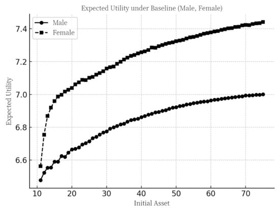
Figure 1.
Maximum expected utility under the baseline scenario.
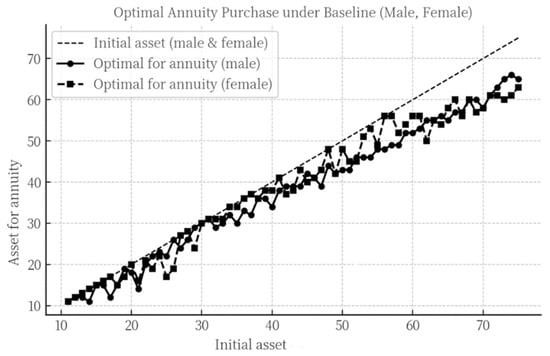
Figure 2.
Optimal annuity purchase decisions under the baseline scenario.
Firstly, as initial assets increase, the expected utility curves for both males and females exhibit the “law of diminishing marginal utility”. In comparison, the overall expected utility for females is higher than that for males. This is because, although females have a higher incidence of disability in old age, their mortality rate is lower, resulting in a longer expected lifespan and, thus, higher overall expected utility.
Secondly, as initial assets increase, the amount allocated to annuity purchases by both males and females generally shows an upward trend, characterized by a “stepwise increase”. Specifically, when an individual has initial assets of (in ten thousand CNY), the amount allocated to annuity purchases is . For each additional CNY 10,000 in initial assets, the annuity purchase amount increases by CNY 0 to 10,000, until the initial assets reach ′. Beyond this point, a further increase of CNY 10,000 in initial assets may actually lead to a decrease in the amount allocated to annuity purchases, after which it resumes its upward trend with further increases in initial assets.
Finally, by observing the separation between the initial asset points and annuity purchase points, it can be seen that as initial assets increase, the proportion of assets allocated to annuity purchases declines for both males and females. Individuals with lower initial assets optimally allocate 100% of their assets to annuity insurance, enabling them to save wealth at an interest rate higher than the market rate and transfer consumption to old age for a greater utility. In contrast, individuals with higher initial assets allocate only a portion of their wealth to annuity insurance, with the remainder being used for current consumption. This is because the marginal utility derived from current consumption exceeds that derived from transferring consumption via annuity purchases, reflecting the overall diminishing marginal utility of annuity insurance. In other words, after annuity purchases reach a certain level, individuals tend to allocate more resources to immediate consumption rather than to further insurance purchases. This preference is partly attributable to the subjective utility discount factor being less than one and partly to the diminishing marginal utility inherent in the utility function.
Furthermore, as this study focuses on the impact of disability risk on annuity purchase decisions, it is necessary to conduct a comparative analysis of with results that exclude the effects of disability risk. Following the aforementioned concept of disability risk, the control variable method is used to examine the isolated impacts of disability-related health costs and disability-related income loss on annuity purchase decisions.
4.1.2. Impact of Disability-Related Health Costs on Annuity Purchase Decisions Under the Baseline Scenario
In the baseline scenario, the disability-related health cost parameter was set to 0 (i.e., ), while all other parameter settings remained unchanged. The model is run again under this configuration, and the relevant results are shown in Figure 3.
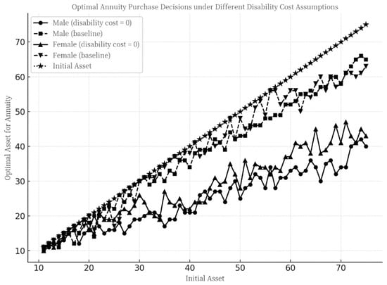
Figure 3.
Optimal annuity purchase decisions under the baseline scenario with disability-related health costs .
As shown in Figure 3, under the scenario where only the disability-related health cost is set to zero while all other settings remain unchanged, the optimal annuity purchase amount still exhibits an overall “stepwise increasing” pattern. However, for both males and females, the assets allocated to annuity purchases deviate to varying degrees compared to the baseline scenario (where disability-related health costs are non-zero).
Specifically, when initial assets are low, individuals tend to allocate almost all their assets to annuity purchases, regardless of whether disability-related health costs are present. However, as the initial assets increase, the optimal annuity purchase amount decreases significantly in the scenario with zero disability-related health costs compared to the case with positive disability-related health costs.
This indicates that, under the baseline scenario, disability-related health costs serve as a significant motivator for annuity purchases among middle-aged males and females around 46 years of age, particularly for those with higher asset levels. This is because that individuals with lower initial assets typically have lower incomes, making it difficult for them to cope with the financial risks associated with disability-related health costs or to maintain high consumption utility in the present. Therefore, regardless of the presence of disability-related health costs, the optimal strategy for this group is to invest all their assets in annuities to achieve asset appreciation and enhance their consumption utility during retirement.
In contrast, for individuals with higher initial assets, when disability-related health costs are zero, their decisions primarily involve intertemporal consumption trade-offs. In this case, the marginal utility of annuity purchases decreases continuously as the amount increases, prompting them to allocate some assets to current consumption to obtain a higher marginal utility. However, when disability-related health costs are present, individuals must not only weigh intertemporal consumption but also prepare for asset depletion shocks due to the disability. This significantly reduces the assets available for consumption in the event of disability, thereby increasing the marginal expected utility derived from annuities, which partially substitutes the marginal utility of current consumption.
4.1.3. The Impact of Disability-Related Income Loss on Annuity Purchase Decisions Under the Baseline Scenario
Under the baseline scenario, the disability-related income loss parameter was set to 0 (), while all other parameter settings remained unchanged, which means if the individual becomes disabled before retirement. The model was executed again under this configuration, and the corresponding results are presented in Figure 4.
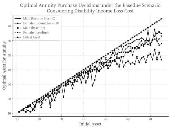
Figure 4.
Optimal annuity purchase decisions under the baseline scenario with disability-related income loss .
As illustrated in Figure 4, under the scenario where only the disability-related income loss is set to zero while all other parameters remain unchanged, the optimal annuity purchase decisions continue to exhibit a “stepwise increasing” pattern. Compared to the results observed when only the disability-related health cost was set to zero, the allocation of assets toward annuity purchases shows only minor deviations from the original baseline.
This result indicates that, in the decision-making process regarding whether and how much to invest in annuities, individuals are primarily motivated by the need to mitigate the impact of disability-related health costs on their lifetime expected utility, while disability-related income loss does not serve as a major influencing factor in this regard. A plausible explanation is that the probability of disability occurring in the middle-aged group between 46 and 65 years old-the pre-retirement stage-is relatively low, and the likelihood of recovery from disability during this period is high. Moreover, because the disability-related income loss in the model is confined to this specific age range, its overall influence on annuity purchase decisions remains limited.
4.2. Model Extension Under Inflation Scenario
4.2.1. Annuity Purchase Decisions Under a Dual-Inflation Scenario
The baseline scenario examines a situation with a 2% annuity yield and zero inflation. Although the increase in China’s national Consumer Price Index (CPI) has been modest in recent years, the growth in medical costs cannot be overlooked. Data show that China’s average CPI over the past five years was 101.77. However, according to the 2024 Global Medical Trends Survey report, China’s medical cost growth rate in 2024 reached 8.35%, indicating that the increase in disability-related health costs significantly outpaced general inflation.
To reflect a more realistic scenario, it is necessary to extend the baseline model by incorporating inflation, particularly the growth in disability-related health costs. First, the minimum consumption level, initial assets, and income in each period are adjusted to 1.0917 times the previous period’s value (approximately equivalent to ). Second, the disability-related health cost in each period is adjusted to 1.4934 times that of the previous period (approximately equal to ). This framework is referred to as the “dual-inflation” model.
By incorporating these adjustments into the model, the annuity purchase decisions under the dual-inflation scenario are derived. The computational results are presented in Figure 5 and Figure 6.
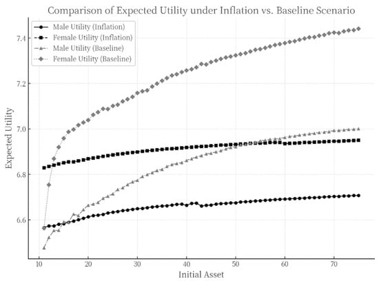
Figure 5.
Comparison of maximum expected utility: dual-inflation scenario vs. baseline scenario.
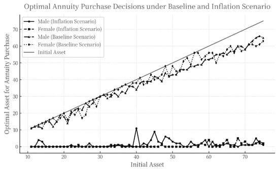
Figure 6.
Comparison of optimal annuity purchase strategies: dual-inflation scenario vs. baseline scenario.
Figure 5 compares the expected utility between the dual-inflation scenario and the baseline scenario for both males and females as initial assets increase. It can be observed that in both cases, expected utility rises with higher initial assets while exhibiting a pattern of “diminishing marginal utility”, consistent with the baseline scenario. As initial assets grow, expected utility under the dual-inflation scenario is significantly lower than that in the baseline scenario across most asset levels, a trend that holds consistently for both genders. This suggests that inflation erodes overall individual welfare, thereby reducing the utility gains derived from initial asset levels and annuity planning.
Notably, however, for individuals with very low initial assets, lifetime expected utility under the dual-inflation scenario is actually higher than in the baseline case.
A further analysis of Figure 6 reveals that, under the inflation scenario, the amount of assets allocated to annuity purchases decreases significantly for both males and females, approaching zero in the vast majority of cases. This finding is consistent with the existing literature. Studies by Hu and Deng and Chen and Fan, based on multi-period life cycle models, also indicate that individuals with initial assets up to CNY 750,000 exhibit zero demand for annuities under inflationary conditions [15,31]. Similarly, Liao et al. observe that the optimal annuity purchase decisions among middle-aged individuals around 45 years old remain at very low levels [28].
Furthermore, the significant divergence in annuity purchase behaviors between the dual-inflation scenario and the baseline scenario carries important practical implications. In the baseline scenario, individuals allocate a relatively high proportion of their assets to annuity insurance regardless of initial wealth levels, whereas under the dual-inflation scenario, annuity purchases are nearly zero.
This phenomenon can be attributed to two main reasons:
- (1)
- The growth rate of disability-related health costs substantially exceeds both the general inflation rate and the annuity yield. This implies that even if individuals invest in annuities, the returns are insufficient to hedge against the financial risks posed by high future health expenditures. With continuously rising medical costs—particularly in the context of a rapidly aging population—the need for health protection becomes increasingly urgent. While annuities can provide certain financial security, their protective effect is limited in the face of rapidly escalating health expenses. Consequently, individuals tend to prioritize allocating resources to mitigate potential disability risks, thereby reducing investment in annuities to avoid future financial distress caused by high health costs.
- (2)
- The annuity yield offers only a limited advantage over the inflation rate, making it difficult for annuity products to provide additional compensatory expected utility to purchasers. This further diminishes individuals’ willingness to purchase annuity insurance.
4.2.2. Optimal Annuity Purchase Decisions Under a Single-Inflation Scenario
The single-inflation model encompasses the following two scenarios:
Scenario 1: Only medical costs due to disability are subject to inflation, while the minimum consumption level, initial assets, and income remain unchanged from the previous period.
Scenario 2: The minimum consumption level, initial assets, and income are adjusted for inflation, while health costs associated with disability are assumed to experience no inflation.
The corresponding results are shown in Figure 7.
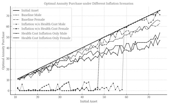
Figure 7.
Optimal annuity purchase decisions under the single-inflation model. (Note: scenario 1: health cost inflation only male and health cost inflation only female. Scenario 2: inflation w/o health cost male and inflation w/o health cost female).
As can be seen from Figure 7, compared to the baseline scenario, the optimal annuity purchase decisions show an overall declining trend when only medical cost inflation due to disability is taken into account (while only , and ). It is worth noting that this effect is not uniformly distributed across all initial asset levels. The higher the initial assets, the more significantly medical cost inflation suppresses the willingness and behavior to purchase annuities, leading high-asset groups to reduce their annuity allocations more markedly when facing such inflationary pressure.
Compared to the dual-inflation scenario discussed earlier, considering only medical cost inflation does not result in drastic changes in annuity purchasing behavior. The reason is that in this scenario, although medical costs grow rapidly, other parameters such as income remain unchanged. This increases the risk of financial insolvency in case of disability, prompting some individuals to maintain or even increase annuity purchases as a form of risk diversification—since annuities can provide a continuous income stream even after financial insolvency occurs.
In contrast, when inflation is applied only to other parameters (such as consumption and income) but not to medical costs (while only ), a different pattern emerges: for individuals with low to medium initial asset levels, annuity purchases decrease significantly and mostly fluctuate near zero, resembling the behavior observed under the full dual-inflation model. However, high-asset individuals almost allocate all their assets to annuity purchases.
This phenomenon can be attributed to two main reasons. First, for high-asset groups, even though the annuity yield offers only a limited advantage over the inflation rate, their large asset base enables them to generate considerable interest income, thereby increasing their willingness to purchase annuities. Second, as indicated in the earlier linear regression analysis, higher initial assets are often associated with higher income. Under the assumption of no inflation in medical costs, these individuals can accumulate wealth steadily through stable income, maintaining high consumption and marginal utility levels. Thus, they are able to both ensure their current quality of life and allocate more resources to future financial security.
On the other hand, for middle- and low-asset groups, the limited improvement of the annuity yield relative to inflation makes it difficult for annuities to provide additional expected utility, which suppresses their demand for such products.
In summary, under inflationary conditions, the limited increase in annuity yields is a key factor restraining demand for annuities among middle- and low-asset groups. High-asset groups, however, are dually affected by rapidly rising medical costs and limited improvement in annuity returns. A single inflationary factor is insufficient to significantly suppress annuity demand among high-asset individuals; only when both factors are present does the inhibitory effect become pronounced.
4.2.3. The Impact of Disability-Related Health Costs on Annuity Purchase Decisions Under Inflation Scenarios
In the baseline scenario, disability-related health costs serve as a significant factor motivating annuity purchases among middle-aged individuals. However, after incorporating inflation into the model, it remains necessary to examine whether the influence of this factor undergoes changes. Under the inflationary scenario, the disability-related health cost parameter is set to 0 while keeping all other settings unchanged (). The model is recalibrated and rerun under this configuration, and the specific computational results are presented in Figure 8.
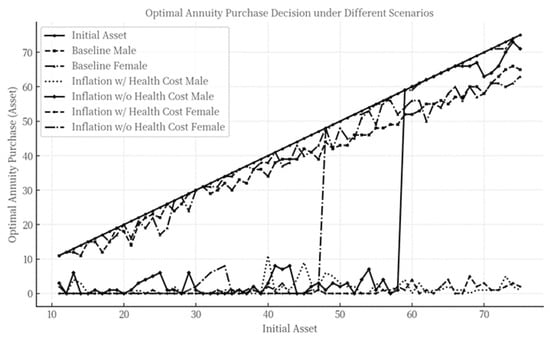
Figure 8.
Optimal annuity purchase decisions under an inflation scenario with disability-related health costs .
As can be observed from Figure 8, under the inflation scenario, the annuity purchase decisions when the disability-related health cost is set to 0 closely resemble those in scenario 2 of the single-inflation model—where disability-related health costs were assumed to experience no inflation.
The reason for this similarity lies in the fact that setting the disability-related health cost to 0 represents a special case of the no-medical-cost-inflation assumption, meaning that health costs remain zero in all periods and do not increase over time. In this situation, the financial impact of disability-related health costs is entirely eliminated. Overall, even under inflationary conditions, assuming disability-related health costs to be zero still significantly suppresses annuity purchases among middle-aged individuals.
4.2.4. The Impact of Disability-Related Income Loss on Annuity Purchase Decisions Under Inflation Scenarios
In the baseline scenario, income loss due to disability shows almost no significant effect on annuity purchase decisions. After introducing inflation into the model, it becomes necessary to examine whether the influence of this factor undergoes any changes. By setting the disability-related income loss parameter to 0 while keeping all other settings unchanged, the model is recalibrated and rerun, which means and if the individual becomes disabled before retirement. The specific computational results are presented in Figure 9.
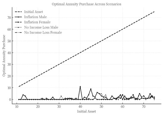
Figure 9.
Optimal annuity purchase decisions under an inflation scenario with disability-related income loss .
As observed in Figure 9, compared to the results derived from the baseline scenario, the annuity purchase decisions under the inflation model exhibit a higher degree of overlap, regardless of whether disability-related income loss is incorporated. Specifically, even when accounting for the potential economic risk of income loss due to disability, its influence on an individual’s decision to purchase annuities appears particularly limited and almost negligible in altering the final outcome. This suggests that, in the presence of inflation, the importance of disability-related income loss as a determinant in annuity purchase decisions is further significantly reduced.
5. Conclusions and Recommendations
5.1. Conclusions
By incorporating health state transition probabilities, disability-related health costs, and disability-related income loss into a multi-period life-cycle model, this study provides an in-depth analysis of annuity purchase decisions among China’s middle-aged population. First, based on CHARLS data, we estimate health state transition probabilities and empirically analyze the correlation between income and assets among the middle-aged population using CHFS data. On this basis, the study examines annuity purchase decisions under a zero-inflation baseline scenario and separately investigates the impact of disability-related health costs and income loss on these decisions.
Furthermore, the model is extended to a more realistic inflation scenario, analyzing the reasons for significant differences in annuity purchase decisions compared to the baseline. Finally, the study quantitatively evaluates the impact of disability-related health costs and income loss on annuity purchase decisions under inflation.
Based on the above analyses, the main conclusions are as follows:
First, there is indeed insufficient demand for annuity products among China’s middle-aged population under current conditions. Specifically, for individuals with low to medium initial assets, the limited increase in annuity yields relative to the inflation rate is the key factor suppressing annuity purchases. Although disability-related health costs are rising rapidly, their inhibitory effect on purchase decisions is less significant than that of inflation.
Second, for those with higher initial assets, the situation differs. The combination of rapidly increasing disability-related health costs and limited improvements in annuity yields serves as an important constraint on annuity purchases. However, with respect to the relationship between annuity yields and inflation, this group exhibits distinct behavioral characteristics: even when annuity yields only marginally outpace inflation, their demand for annuity products is not suppressed and may even be stimulated.
This behavioral divergence can be partially explained by the heterogeneity in risk and time preferences from behavioral economics: the low-to-medium asset group, facing stricter budget constraints, is motivated primarily by the need for asset appreciation when purchasing annuities, thus showing greater sensitivity to the cost of purchase (i.e., the yield–inflation gap). In contrast, the high-asset group views annuities not only as a long-term wealth planning tool but also as a means to hedge against longevity-related disability risks. As a result, a single unfavorable factor change is unlikely to significantly influence their decision-making.
It is noteworthy that, regardless of the initial asset level, disability-related income loss has almost no impact on annuity purchase decisions for the middle-aged population. This conclusion holds in both inflationary and non-inflationary scenarios, indicating that, when making annuity purchase decisions, the middle-aged group is more focused on factors such as health costs rather than the loss of income due to disability.
Moreover, comparing the scenarios with and without inflation reveals significant changes in annuity purchase behavior. Under the baseline scenario with zero inflation, almost all middle-aged individuals tend to allocate the vast majority of their assets to annuity purchases. In this case, disability-related health costs become an important factor influencing decisions at different asset levels, with their impact increasing as initial assets rise. This suggests that, in the absence of inflationary pressure, disability-related health costs are particularly critical for those with higher asset levels, who are more likely to adjust their annuity purchase strategies in response to changes in these costs.
In summary, the relative relationship between inflation and annuity yields, as well as the growth of disability-related health costs, are core variables influencing annuity purchase decisions among China’s middle-aged population. Additionally, the study reveals that, under certain conditions (such as zero inflation), behavioral patterns may undergo fundamental shifts, offering important insights for relevant policy-making and product design.
5.2. Recommendations for Optimizing Annuity Products
Currently, annuity purchase decisions among China’s middle-aged population exhibit significant stratification, shaped by the complex interplay of initial asset levels, health costs, inflation, and annuity yields. Based on the empirical analysis from the multi-period life-cycle model, the following policy recommendations are proposed:
5.2.1. Differentiated Product Design to Meet Layered Needs
It is important to address the middle-aged group’s high sensitivity to the gap between inflation and annuity yields. For the low- and middle-asset groups, it is recommended that insurers develop inflation-protected annuity products by linking annuity payments to inflation indices (such as the CPI) or dynamically adjusting payment amounts. This would help mitigate the suppressive effect of the yield–inflation gap on purchase decisions. At the same time, the mechanism for forming annuity yields should be optimized to enhance long-term investment capabilities; diversified asset allocation can be used to boost yields and narrow the gap with inflation. A profit-sharing mechanism could be introduced, returning a portion of excess investment returns to policyholders to enhance product attractiveness. Additionally, drawing on the premium payment structure of universal life insurance, a tiered premium payment plan could be designed, allowing for low-threshold initial entry and flexible subsequent top-ups, thereby reducing the financial burden for low- and middle-asset groups.
For the high-asset group, under expectations of low inflation and rapidly rising health costs, annuity purchase willingness is significantly constrained. To address this, it is recommended to embed disability risk management functions in product design, aiming to reduce the expected value of future health expenditures. On one hand, annuity payments can be linked with long-term care costs, developing hybrid products that combine annuities with long-term care insurance, thereby providing dual protection against disability risk and indirectly alleviating the pressure of rising health costs, or integrating medical resources to lower expected future medical expenditures. On the other hand, insurers could combine health management services (such as regular check-ups and disease prevention) with annuity products, providing health management support to help reduce the probability of future disability, further enhancing annuity purchase willingness among high-asset individuals.
5.2.2. Institutional Contingency Plans for Zero Inflation Scenarios
In a zero-inflation scenario, annuity purchase behavior among the middle-aged may shift abruptly, leading to surges in demand and even excessive allocation of assets to annuity products. Thus, product and regulatory design should balance risk prevention and market stability, focusing on reconciling individual rational decisions with systemic risk.
First, a dynamic liquidity management mechanism should be established, requiring insurers to adjust reserve standards in response to macroeconomic conditions. For instance, simulating annuity payout stress under extreme deflation scenarios and limiting investment in high-risk assets to prevent liquidity crises triggered by surging demand. Second, the counter-cyclical regulatory framework should be optimized, with temporary relaxation of minimum yield requirements for annuity products during deflationary periods, alongside actuarial balance constraints. Insurers should regularly assess the match between actual yields and promised benefits, and when deviations exceed a threshold, an automatic adjustment mechanism for benefit payments should be triggered to avoid the accumulation of long-term interest rate spread losses.
To address the risk of individual over-allocation, a cap could be set on the proportion of annuity premiums relative to disposable assets, with real-time monitoring achieved through banking and insurance data integration. For purchases exceeding the threshold, a mandatory financial health assessment process should be initiated, with an independent third party reviewing the policyholder’s asset-liability structure and short-term liquidity needs to guard against personal financial risks arising from excessive annuity allocation.
5.3. Limitations and Future Research
This paper applies a dynamic programming algorithm to solve the optimal annuity purchase decision problem for the middle-aged population, which leads to certain limitations and shortcomings in this study. First, the dynamic programming algorithm lacks a standardized solution template. In practical applications, it requires deeply integrating the characteristics of the problem to design tailored solutions. As a result, this study can only obtain numerical solutions rather than closed-form solutions. Additionally, as the dimensionality of variables increases, the total computational and storage requirements grow exponentially. Consequently, due to constraints in computer storage and processing speed, modern computers still cannot use dynamic programming methods to solve large-scale problems, a phenomenon known as the “curse of dimensionality”. To mitigate this issue, this study adopts certain methods to reduce dimensionality and accelerate iterative computations, such as setting state transitions to occur at 5-year intervals and discretizing continuous variables like income and assets. However, these approaches come at the cost of reduced precision. Future research could enhance solution accuracy with advancements in computer technology, for example, by increasing the frequency of state transitions and reducing the degree of discretization for continuous variables.
Author Contributions
Methodology, Z.X.; software, Z.X.; validation, L.S.; formal analysis, L.S.; investigation, L.S.; resources, X.Y.; data curation, Z.X.; writing—original draft preparation, Z.X.; writing—review visualization, X.Y.; supervision, X.Y.; All authors have read and agreed to the published version of the manuscript.
Funding
This research received no external funding.
Data Availability Statement
The original contributions presented in the study are included in the article material. Further inquiries can be directed to the corresponding author.
Conflicts of Interest
Author Spyridon Louvros was employed by the company Mobile Cloud Network & Services. The author declare that the research was conducted in the absence of any commercial or financial relationships that could be construed as a potential conflict of interest. The company Mobile Cloud Network & Services had no role in the design of the study; in the collection, analyses, or interpretation of data; in the writing of the manuscript, or in the decision to publish the results.
Appendix A

Table A1.
Descriptive statistics of income and assets.
Table A1.
Descriptive statistics of income and assets.
| Variables | Sample Size | Mean | Standard Deviation | Minimum | Maximum |
|---|---|---|---|---|---|
| Income | 1061 | 38,740.07 | 50,581.55 | 10,000.44 | 726,434.4 |
| Initial Assets | 1061 | 451,589.8 | 761,636.3 | 10,069.67 | 8,623,458 |
Table A2.
Regression results of the model.
Table A2.
Regression results of the model.
| Variables | Estimated Coefficients | Standard Deviation | p Value |
|---|---|---|---|
| 0.3122366 | 0.0140144 | 0.000 | |
| Constant | 6.431887 | 0.1720796 | 0.000 |
Table A3.
Two-year health state transition probabilities for ages 46–85.
Table A3.
Two-year health state transition probabilities for ages 46–85.
| Two-Year Health State Transition Probability Matrix for Ages 46–55 | |||||||||
|---|---|---|---|---|---|---|---|---|---|
| Terminal | Healthy | Mildly Disabled | Severely Disabled | Death | |||||
| Initial | Male | Female | Male | Female | Male | Female | Male | Female | |
| Healthy | 0.9034 | 0.8261 | 0.0654 | 0.1196 | 0.0254 | 0.0519 | 0.0058 | 0.0024 | |
| Mildly disabled | 0.6875 | 0.5855 | 0.1875 | 0.2565 | 0.1094 | 0.1554 | 0.0156 | 0.0026 | |
| Severely disabled | 0.3784 | 0.3267 | 0.2072 | 0.1633 | 0.3784 | 0.4821 | 0.0360 | 0.0279 | |
| Death | 0.0000 | 0.0000 | 0.0000 | 0.0000 | 0.0000 | 0.0000 | 1.0000 | 1.0000 | |
| Two-Year Health State Transition Probability Matrix for Ages 56–65 | |||||||||
| Terminal | Healthy | Mildly disabled | Severely disabled | Death | |||||
| Initial | Male | Female | Male | Female | Male | Female | Male | Female | |
| Healthy | 0.8254 | 0.7613 | 0.1138 | 0.1528 | 0.0487 | 0.0790 | 0.0121 | 0.0069 | |
| Mildly disabled | 0.5841 | 0.5000 | 0.2389 | 0.2857 | 0.1327 | 0.2068 | 0.0442 | 0.0075 | |
| Severely disabled | 0.2137 | 0.2121 | 0.1694 | 0.2283 | 0.5282 | 0.5313 | 0.0887 | 0.0283 | |
| Death | 0.0000 | 0.0000 | 0.0000 | 0.0000 | 0.0000 | 0.0000 | 1.0000 | 1.0000 | |
| Two-Year Health State Transition Probability Matrix for Ages 66–75 | |||||||||
| Terminal | Healthy | Mildly disabled | Severely disabled | Death | |||||
| Initial | Male | Female | Male | Female | Male | Female | Male | Female | |
| Healthy | 0.7547 | 0.6596 | 0.1541 | 0.1974 | 0.0621 | 0.1238 | 0.0292 | 0.0192 | |
| Mildly disabled | 0.4645 | 0.4357 | 0.2663 | 0.2946 | 0.2041 | 0.2448 | 0.0651 | 0.0249 | |
| Severely disabled | 0.1311 | 0.1621 | 0.1860 | 0.1971 | 0.5427 | 0.5838 | 0.1402 | 0.0571 | |
| Death | 0.0000 | 0.0000 | 0.0000 | 0.0000 | 0.0000 | 0.0000 | 1.0000 | 1.0000 | |
| Two-Year Health State Transition Probability Matrix for Ages 76–85 | |||||||||
| Terminal | Healthy | Mildly disabled | Severely disabled | Death | |||||
| Initial | Male | Female | Male | Female | Male | Female | Male | Female | |
| Healthy | 0.6082 | 0.5652 | 0.1881 | 0.2174 | 0.1285 | 0.1696 | 0.0752 | 0.0478 | |
| Mildly disabled | 0.2973 | 0.3086 | 0.3108 | 0.3025 | 0.2905 | 0.3333 | 0.1014 | 0.0556 | |
| Severely disabled | 0.1415 | 0.1051 | 0.1317 | 0.1797 | 0.4585 | 0.5593 | 0.2683 | 0.1559 | |
| Death | 0.0000 | 0.0000 | 0.0000 | 0.0000 | 0.0000 | 0.0000 | 1.0000 | 1.0000 | |
Table A4.
Five-year health state transition probability.
Table A4.
Five-year health state transition probability.
| Five-Year Health State Transition Probability Matrix for Ages 46–55 | |||||||||
|---|---|---|---|---|---|---|---|---|---|
| Terminal | Healthy | Mildly Disabled | Severely Disabled | Death | |||||
| Initial | Male | Female | Male | Female | Male | Female | Male | Female | |
| Healthy | 0.8613 | 0.7547 | 0.0785 | 0.1404 | 0.0433 | 0.0963 | 0.0169 | 0.0085 | |
| Mildly disabled | 0.8075 | 0.6996 | 0.0927 | 0.1512 | 0.0686 | 0.1370 | 0.0312 | 0.0122 | |
| Severely disabled | 0.6912 | 0.5783 | 0.1193 | 0.1535 | 0.1278 | 0.2205 | 0.0617 | 0.0477 | |
| Death | 0.0000 | 0.0000 | 0.0000 | 0.0000 | 0.0000 | 0.0000 | 1.0000 | 1.0000 | |
| Five-Year Health State Transition Probability Matrix for Ages 56–65 | |||||||||
| Terminal | Healthy | Mildly disabled | Severely disabled | Death | |||||
| Initial | Male | Female | Male | Female | Male | Female | Male | Female | |
| Healthy | 0.7364 | 0.6477 | 0.1308 | 0.1821 | 0.0905 | 0.1499 | 0.0422 | 0.0203 | |
| Mildly disabled | 0.6524 | 0.5755 | 0.1359 | 0.1969 | 0.1248 | 0.2029 | 0.0868 | 0.0247 | |
| Severely disabled | 0.4411 | 0.4417 | 0.1431 | 0.2091 | 0.2490 | 0.2953 | 0.1668 | 0.0539 | |
| Death | 0.0000 | 0.0000 | 0.0000 | 0.0000 | 0.0000 | 0.0000 | 1.0000 | 1.0000 | |
| Five-Year Health State Transition Probability Matrix for Ages 66–75 | |||||||||
| Terminal | Healthy | Mildly disabled | Severely disabled | Death | |||||
| Initial | Male | Female | Male | Female | Male | Female | Male | Female | |
| Healthy | 0.6131 | 0.5074 | 0.1681 | 0.2117 | 0.1264 | 0.2236 | 0.0924 | 0.0573 | |
| Mildly disabled | 0.4961 | 0.4484 | 0.1688 | 0.2128 | 0.1831 | 0.2693 | 0.1520 | 0.0695 | |
| Severely disabled | 0.2934 | 0.3226 | 0.1587 | 0.2017 | 0.2801 | 0.3597 | 0.2678 | 0.1161 | |
| Death | 0.0000 | 0.0000 | 0.0000 | 0.0000 | 0.0000 | 0.0000 | 1.0000 | 1.0000 | |
| Five-Year Health State Transition Probability Matrix for Ages 76–85 | |||||||||
| Terminal | Healthy | Mildly disabled | Severely disabled | Death | |||||
| Initial | Male | Female | Male | Female | Male | Female | Male | Female | |
| Healthy | 0.3933 | 0.3583 | 0.1794 | 0.2107 | 0.2003 | 0.2817 | 0.2269 | 0.1494 | |
| Mildly disabled | 0.3015 | 0.2887 | 0.1685 | 0.2039 | 0.2377 | 0.3277 | 0.2923 | 0.1797 | |
| Severely disabled | 0.1942 | 0.1880 | 0.1194 | 0.1698 | 0.2177 | 0.3425 | 0.4687 | 0.2997 | |
| Death | 0.0000 | 0.0000 | 0.0000 | 0.0000 | 0.0000 | 0.0000 | 1.0000 | 1.0000 | |
References
- Yaari, M.E. Uncertain lifetime, life insurance, and the theory of the consumer. Rev. Econ. Stud. 1965, 32, 137–150. [Google Scholar] [CrossRef]
- Schaus, S. Annuities make a comeback. J. Pension Benefits Issues Adm. 2005, 12, 34–38. [Google Scholar]
- Inkmann, J.; Lopes, P.; Michaelides, A. How deep is the annuity market participation puzzle? Rev. Financ. Stud. 2011, 24, 279–319. [Google Scholar] [CrossRef]
- Modigliani, F.; Brumberg, R. Utility Analysis and the Consumption Function: An Interpretation of Cross-Section Data. In Post-Keynesian Economics; Kurihara, K.K., Ed.; Rutgers University Press: New Brunswick, NJ, USA, 1954; pp. 388–436. [Google Scholar]
- Samuelson, P.A. Lifetime Portfolio Selection by Dynamic Stochastic Programming. Rev. Econ. Stat. 1969, 51, 239–246. [Google Scholar] [CrossRef]
- Merton, R.C. Lifetime Portfolio Selection: The Continuous-Time Case. Rev. Econ. Stat. 1969, 51, 247–257. [Google Scholar] [CrossRef]
- Merton, R.C. Optimum Consumption and Portfolio Rules in a Continuous-Time Model. J. Econ. Theory 1971, 3, 373–413. [Google Scholar] [CrossRef]
- Gourinchas, P.-O.; Parker, J.A. Consumption over the Life Cycle. Econometrica 2002, 70, 47–89. [Google Scholar] [CrossRef]
- Hubbard, R.G.; Skinner, J.; Zeldes, S.P. Precautionary saving and social insurance. J. Political Econ. 1995, 103, 360–399. [Google Scholar] [CrossRef]
- Mitchell, O.S.; Poterba, J.; Warshawsky, M.; Brown, J. New Evidence on the Money’s Worth of Individual Annuities. Am. Econ. Rev. 1999, 89, 1299–1318. [Google Scholar] [CrossRef]
- De Nardi, M.; French, E.; Jones, J.B. Why do the elderly save? The role of medical expenses. J. Political Econ. 2010, 118, 39–75. [Google Scholar] [CrossRef]
- Lewis, F.D. Dependents and the Demand for Life Insurance. Am. Econ. Rev. 1989, 79, 452–467. [Google Scholar]
- Reichling, F.; Smetters, K. Optimal annuitization with stochastic mortality and correlated medical costs. J. Am. Econ. Rev. 2015, 105, 3273–3320. [Google Scholar] [CrossRef]
- Peijnenburg, K.; Nijman, T.; Werker, B.J.M. Health cost risk: A potential solution to the annuity puzzle. Econ. J. 2017, 127, 1598–1625. [Google Scholar] [CrossRef]
- Chen, B.Z.; Fan, C. The impact of health risks on annuity demand among the elderly in China. Insur. Stud. 2020, 9, 52–63. [Google Scholar]
- Yogo, M. Portfolio Choice in Retirement: Health risk and the demand for annuities, housing, and risky assets. J. Monet. Econ. 2016, 80, 17–34. [Google Scholar] [CrossRef]
- Timo, R.L.; Frederik, T.S. Displaced, disliked and misunderstood: A systematic review of the reasons for low uptake of long-term care insurance and life annuities. J. Econ. Ageing 2020, 17, 100236. [Google Scholar] [CrossRef]
- Cui, X.D.; Zhou, H.H.; Zhu, Y.M.; Chen, P.W. Longevity and health: A verification based on a state-transition probability model. Stat. Res. 2022, 39, 134–146. (In Chinese) [Google Scholar]
- Pang, G.; Warshawsky, M. Optimizing the equity-bond-annuity portfolio in retirement: The impact of uncertain health expenses. Insur. Math. Econ. 2010, 46, 198–209. [Google Scholar] [CrossRef]
- Ai, J.; Brockett, P.L.; Golden, L.L.; Zhu, W. Health state transitions and longevity effects on retirees’ optimal annuitization. J. Risk Insur. 2017, 84, 319–343. [Google Scholar] [CrossRef]
- Koijen, R.S.J.; Van Nieuwerburgh, S.; Yogo, M. Health and mortality delta: Assessing the welfare cost of household insurance choice. J. Financ. 2016, 71, 957–1010. [Google Scholar] [CrossRef]
- Hambel, C.; Kraft, H.; Schendel, L.S.; Steffensen, M. Life insurance demand under health shock risk. J. Risk Insur. 2017, 84, 1171–1202. [Google Scholar] [CrossRef]
- Ameriks, J.; Briggs, J.; Caplin, A.; Shapiro, M.D.; Tonetti, C. Long-term-care utility and late-in-life saving. J. Political Econ. 2020, 128, 2375–2451. [Google Scholar] [CrossRef]
- Hambel, C. Health shock risk, critical illness insurance, and housing services. Insur. Math. Econ. 2020, 91, 111–128. [Google Scholar] [CrossRef]
- Chen, X.B.; Fu, D.S.; Ge, C.J. A dynamic optimization simulation of consumption and investment behavior over the life cycle of Chinese residents. J. Financ. Res. 2006, 21–35. (In Chinese) [Google Scholar]
- Chen, C.C.; Chang, C.C.; Sun, E.W.; Yu, M.T. Optimal decision of dynamic wealth allocation with life insurance for mitigating health risk under market incompleteness. Eur. J. Oper. Res. 2022, 300, 727–742. [Google Scholar] [CrossRef]
- Ren, Z.P. China Aging Report. Dev. Res. 2023, 40, 22–30. [Google Scholar]
- Liao, P.; Yang, H.Q.; Huang, X.Y. Optimal allocation of personal insurance under health risks. Chin. J. Manag. Sci. 2023, 32, 61–73. [Google Scholar]
- Bellman, R. The theory of dynamic programming. Bull. Am. Math. Soc. 1954, 60, 503–516. [Google Scholar] [CrossRef]
- Carroll, C.D. The method of endogenous gridpoints for solving dynamic stochastic optimization problems. Econ. Lett. 2006, 91, 312–320. [Google Scholar] [CrossRef]
- Hu, X.; Deng, R.H. Analysis of the impact of health risk and longevity risk on residents’ optimal annuity and long-term care insurance decisions. In Proceedings of the International Conference on Insurance and Risk Management (CICIRM 2023), Guangzhou, China, 12–15 July 2023; pp. 72–87. [Google Scholar]
- Wang, X.J.; Wang, J.Y. Pricing of long-term care insurance based on a Markov Model. Insur. Stud. 2018, 10, 87–99. [Google Scholar]
- Song, Z.; Storesletten, K.; Zilibotti, F. Growing like China. Am. Econ. Rev. 2011, 101, 196–233. [Google Scholar] [CrossRef]
- Ai, C.R.; Wang, W. Excess sensitivity of Chinese household consumption under habit formation: An analysis based on interprovincial dynamic panel data from 1995 to 2005. J. Quant. Technol. Econ. 2008, 25, 98–114. [Google Scholar]


Disclaimer/Publisher’s Note: The statements, opinions and data contained in all publications are solely those of the individual author(s) and contributor(s) and not of MDPI and/or the editor(s). MDPI and/or the editor(s) disclaim responsibility for any injury to people or property resulting from any ideas, methods, instructions or products referred to in the content. |
© 2025 by the authors. Licensee MDPI, Basel, Switzerland. This article is an open access article distributed under the terms and conditions of the Creative Commons Attribution (CC BY) license (https://creativecommons.org/licenses/by/4.0/).