Controlled Filtered Poisson Processes

Abstract

Filtered Poisson processes are used as models in various applications, in particular in statistical hydrology. In this paper, controlled filtered Poisson processes are considered. The aim is to minimize the expected time that the process will spend in the continuation region. The dynamic programming equation satisfied by the value function is derived. To obtain the value function, and hence the optimal control, a non-linear integro-differential equation must be solved, subject to the appropriate boundary conditions. Various cases for the size of the jumps are treated and explicit results are obtained.

1. Introduction

Let $\left\{X\right(t),t\ge 0\}$ be the stochastic process defined by

$$X\left(t\right)=x+\sum _{k=1}^{N\left(t\right)}w(t,T_k,Y_k),$$

(1)

where $x=X\left(0\right)$, $\left\{N\right(t),t\ge 0\}$ is a Poisson process with rate or intensity $\lambda$ and $w(·,·,·)$ is called the response function. The random variables $T_1,T_2,\dots$ are the arrival times of the events of the Poisson process, and $\{Y_1,Y_2,\dots \}$ is a sequence of independent random variables that are identically distributed as a random variable Y.

The process $\left\{X\right(t),t\ge 0\}$ is known as a filtered Poisson process (FPP); see [1] (p. 145). It has applications in various fields. In [2], Lefebvre and Guilbault used these processes to model a river flow. The authors also estimated return periods in hydrology based on FPPs.

In hydrology, an appropriate response function is of the form

$$w(t,T_k,Y_k)=Y_k{e}^{-(t-T_k)/c},$$

(2)

where c is a positive constant. This is the response function that will be used in this paper.

Remark 1.

Notice that with the response function defined in Equation (2), we can express $X(t+\Delta t)$ in terms of $X\left(t\right)$:

$$\begin{array}{ccc}\hfill X(t+\Delta t)& =& x+\sum _{k=1}^{N(t+\Delta t)}{Y}_k{e}^{-(t+\Delta t-T_k)/c}\hfill \\ & =& x+\sum _{k=1}^{N\left(t\right)}{Y}_k{e}^{-(t+\Delta t-T_k)/c}+\sum _{k=N\left(t^{+}\right)}^{N(t+\Delta t)}{Y}_k{e}^{-(t+\Delta t-T_k)/c}\hfill \\ & =& e^{-\Delta t}\left[X\left(t\right)-x\right]+\sum _{k=N\left(t^{+}\right)}^{N(t+\Delta t)}{Y}_k{e}^{-(t+\Delta t-T_k)/c}.\hfill \end{array}$$

(3)

Moreover, since the Poisson process $\left\{N\right(t),t\ge 0\}$ has independent increments, the summation in the above equation is independent of $X\left(t\right)$.

Filtered Poisson processes have applications in physics, operation research, finance and actuarial science, among other fields. Many theoretical and applied papers have been written on FPPs or generalizations of these processes. Racicot and Moses [3] used FPPs in vibration problems. Hero [4] estimated the time shift of a non-homogeneous FPP in the presence of additive Gaussian noise. Grigoriu [5] developed methods in order to find properties of the output of linear and non-linear dynamic systems to random actions represented by FPPs. Novikov et al. [6] considered first-passage problems for FPPs. Yin et al. [7] modelled snow loads as FPPs. Theodorsen et al. [8] obtained statistical properties of an FPP with additive random noise. Alazemi et al. [9] computed estimators of FPP intensities. In Grant and Szechtman [10], the process $\left\{N\right(t),t\ge 0\}$ is replaced by a non-homogeneous Poisson process.

In this paper, we consider a controlled version of $\left\{X\right(t),t\ge 0\}$:

$$X\left(t\right)=x+b_0{\int }_0^{t}u\left[X\left(s\right)\right]\mathrm{d}s+\sum _{k=1}^{N\left(t\right)}{Y}_k{e}^{-(t-T_k)/c},$$

(4)

where $b_0$ is a positive constant and the control $u(·)$ is assumed to be a continuous function.

Let $\tau \left(x\right)$ be the first-passage time random variable defined by

$$\tau \left(x\right)=inf\{t\ge 0:X(t)\ge d\mid X(0)=x\},$$

(5)

where $x\le d$. Our aim is to minimize the expected value of the cost function

$$J\left(x\right):={\int }_0^{\tau \left(x\right)}\left\{{\displaystyle \frac{1}{2}}{q}_0{u}^2\left[X\left(t\right)\right]+\theta \right\}\mathrm{d}t+K\left[X\left(\tau \left(x\right)\right)\right],$$

(6)

where $q_0$ and $\theta$ are positive constants and $K(·)$ is the terminal cost function. Because the parameter $\theta$ is positive, the optimizer wants to minimize the expected time that the controlled process will spend in the interval $(-\infty ,d)$, while taking into account the quadratic control costs and the terminal cost. We could assume instead that $\theta$ is negative, so that the objective would be to maximize the expected time in the continuation region $(-\infty ,d)$.

This type of problem, in which the optimizer controls a stochastic process until a certain event occurs, is known as a homing problem. Whittle [11] has considered these problems for n-dimensional diffusion processes. In [12], he generalized the cost criterion by taking the risk-sensitivity of the optimizer into account.

The author has written numerous papers on homing problems for different types of stochastic processes. Recently, he and Yaghoubi have solved homing problems for queueing systems and for continuous-time Markov chains; see [13].

Next, we define the value function

$$F\left(x\right)=\underset{\begin{array}{c}u\left[X\right(t\left)\right]\\ t\in [0,\tau (x\left)\right)\end{array}}{inf}E\left[J\left(x\right)\right].$$

(7)

It gives the expected cost obtained if the optimizer chooses the optimal value of the control $u\left[X\right(t\left)\right]$ in the interval $[0,\tau (x\left)\right)$.

In Section 2, the dynamic programming equation satisfied by the value function will be derived. Then, in Section 3, various cases for the distribution of the random variable Y, which denotes the size of the jumps, will be considered. Explicit results will be obtained for the value function and the optimal control. To do so, we will have to solve a non-linear integro-differential equation.

2. Dynamic Programming Equation

We have, for $x<d$,

$$\begin{array}{ccc}\hfill F\left(x\right)& :=& \underset{\begin{array}{c}u\left[X\right(t\left)\right]\\ t\in [0,\tau (x\left)\right)\end{array}}{inf}E\left[J\left(x\right)\right]=\underset{\begin{array}{c}u\left[X\right(t\left)\right]\\ t\in [0,\tau (x\left)\right)\end{array}}{inf}E\left[{\int }_0^{\tau \left(x\right)}\left\{{\displaystyle \frac{1}{2}}{q}_0{u}^2\left[X\left(t\right)\right]+\theta \right\}\mathrm{d}t\right]\hfill \\ & =& \underset{\begin{array}{c}u\left[X\right(t\left)\right]\\ t\in [0,\tau (x\left)\right)\end{array}}{inf}E\left[{\int }_0^{\Delta t}\left\{{\displaystyle \frac{1}{2}}{q}_0{u}^2\left[X\left(t\right)\right]+\theta \right\}\mathrm{d}t+{\int }_{\Delta t}^{\tau \left(x\right)}\left\{{\displaystyle \frac{1}{2}}{q}_0{u}^2\left[X\left(t\right)\right]+\theta \right\}\mathrm{d}t\right].\hfill \end{array}$$

(8)

For a $\Delta t$ that is small,

$${\int }_0^{\Delta t}\left\{{\displaystyle \frac{1}{2}}{q}_0{u}^2\left[X\left(t\right)\right]+\theta \right\}\mathrm{d}t=\left\{{\displaystyle \frac{1}{2}}{q}_0{u}^2\left(x\right)+\theta \right\}\Delta t+o(\Delta t).$$

(9)

Moreover, using Bellman’s principle of optimality (see [14]), we can express the second integral in Equation (8) in terms of the value function:

$$\underset{\begin{array}{c}u\left[X\right(t\left)\right]\\ t\in [\Delta t,\tau (x\left)\right)\end{array}}{inf}E\left[{\int }_{\Delta t}^{\tau \left(x\right)}\left\{{\displaystyle \frac{1}{2}}{q}_0{u}^2\left[X\left(t\right)\right]+\theta \right\}\mathrm{d}t\right]=E\left[F\left(X(\Delta t)\right)\right]+o(\Delta t),$$

(10)

where

$$X(\Delta t)=x+b_{0}u\left(x\right)\Delta t+\sum _{k=1}^{N(\Delta t)}{Y}_k{e}^{-(\Delta t-T_k)/c}+o(\Delta t).$$

(11)

It follows that it is sufficient to find the optimal value of the control $u\left[X\right(t\left)\right]$ at the initial instant:

$$F\left(x\right)=\underset{u\left(x\right)}{inf}\left\{\left({\displaystyle \frac{1}{2}}{q}_0{u}^2\left(x\right)+\theta \right)\Delta t+E\left[F\left(X(\Delta t)\right)\right]\right\}+o(\Delta t).$$

(12)

Next,

$$P[N(\Delta t)=k]=\left\{\begin{array}{cc}1-\lambda \Delta t+o(\Delta t)& \mathrm{if}k=0,\hfill \\ \lambda \Delta t+o(\Delta t)& \mathrm{if}k=1,\hfill \end{array}\right.$$

(13)

so that

$$P\left[N\right(\Delta t)\ge 2]=o(\Delta t).$$

(14)

Hence, we can write that

$$X(\Delta t)=\left\{\begin{array}{cc}x+b_{0}u\left(x\right)\Delta t+o(\Delta t)& \mathrm{with}\mathrm{probability}1-\lambda \Delta t+o(\Delta t),\hfill \\ x+b_{0}u\left(x\right)\Delta t+Y_1{e}^{-(\Delta t-T_1)/c}+o(\Delta t)& \mathrm{with}\mathrm{probability}\lambda \Delta t+o(\Delta t).\hfill \end{array}\right.$$

(15)

Now, we have

$$P[N(\Delta t)=1]=P[T_1\le \Delta t]+o(\Delta t)$$

(16)

and

$$T_1\mid \{T_1\le \Delta t\}\sim \mathrm{U}(0,\Delta t],$$

(17)

where $T_1$ is the arrival time of the first event of the Poisson process $\left\{N\right(t),t\ge 0\}$. That is, given that $T_1\le \Delta t$, the random variable $T_1$ has a uniform distribution on the interval $(0,\Delta t]$. It follows, making use of the law of total probability for continuous random variables, that

$$\begin{array}{ccc}\hfill E\left[F\left(X(\Delta t)\right)\right]& =& F\left[x+b_{0}u\left(x\right)\Delta t\right][1-\lambda \Delta t+o(\Delta t)]\hfill \\ & & +{\int }_{-\infty }^{\infty }{\int }_0^{\Delta t}F\left[x+b_{0}u\left(x\right)\Delta t+y{e}^{-(\Delta t-s)/c}\right]{\displaystyle \frac{1}{\Delta t}}{f}_Y\left(y\right)\mathrm{d}s\mathrm{d}y\hfill \\ & & \times [\lambda \Delta t+o(\Delta t\left)\right]+o(\Delta t),\hfill \end{array}$$

(18)

where $f_Y\left(y\right)$ is the probability density function of the random variable Y (the parent random variable of $Y_1,Y_2,\dots$).

We deduce from Taylor’s theorem that

$$F\left[x+b_{0}u\left(x\right)\Delta t\right]=F\left(x\right)+b_{0}u\left(x\right)\Delta t{F}^{\prime }\left(x\right)+o(\Delta t).$$

(19)

Furthermore,

$$e^{-(\Delta t-s)/c}=e^{s/c}\left[1-{\displaystyle \frac{\Delta t}{c}}+o(\Delta t)\right],$$

(20)

which implies that

$${\int }_0^{\Delta t}{e}^{-(\Delta t-s)/c}\mathrm{d}s=c\left[e^{\Delta t/c}-1\right]\left[1-{\displaystyle \frac{\Delta t}{c}}+o(\Delta t)\right]=\Delta t+o(\Delta t).$$

(21)

Similarly,

$${\int }_0^{\Delta t}{e}^{-k(\Delta t-s)/c}\mathrm{d}s={\displaystyle \frac{c}{k}}\left[e^{k\Delta t/c}-1\right]\left[1-{\displaystyle \frac{k\Delta t}{c}}+o(\Delta t)\right]=\Delta t+o(\Delta t)$$

(22)

for any $k\in \mathbb{N}$. Hence,

$$\begin{array}{ccc}\hfill {\int }_0^{\Delta t}F\left[x+b_{0}u\left(x\right)\Delta t+y{e}^{-(\Delta t-s)/c}\right]\mathrm{d}s& =& F\left(x\right)\Delta t+b_{0}u\left(x\right){(\Delta t)}^2{F}^{\prime }\left(x\right)\hfill \\ & & +y\Delta t{F}^{\prime }\left(x\right)+{\displaystyle \frac{y^2}{2}}\Delta t{F}^{″}\left(x\right)+\dots +o(\Delta t)\hfill \\ & =& F\left(x\right)\Delta t+b_{0}u\left(x\right){(\Delta t)}^2{F}^{\prime }\left(x\right)\hfill \\ & & +\left[F(x+y)-F\left(x\right)\right]\Delta t+o(\Delta t).\hfill \end{array}$$

(23)

From what precedes, we may write that

$$\begin{array}{ccc}\hfill F\left(x\right)& =& \underset{u\left(x\right)}{inf}\{\left({\displaystyle \frac{1}{2}}{q}_0{u}^2\left(x\right)+\theta \right)\Delta t+\left[F\left(x\right)+b_{0}u\left(x\right)\Delta t{F}^{\prime }\left(x\right)+o(\Delta t)\right][1-\lambda \Delta t+o(\Delta t)]\hfill \\ & & +\left[F\left(x\right)+b_{0}u\left(x\right)\Delta t{F}^{\prime }\left(x\right)+{\int }_{-\infty }^{\infty }\left[F(x+y)-F\left(x\right)\right]f_Y\left(y\right)\mathrm{d}y+o(\Delta t)\right]\hfill \\ & & \times [\lambda \Delta t+o(\Delta t\left)\right]\}+o(\Delta t).\hfill \end{array}$$

(24)

That is,

$$\begin{array}{ccc}\hfill 0& =& \underset{u\left(x\right)}{inf}\{\left({\displaystyle \frac{1}{2}}{q}_0{u}^2\left(x\right)+\theta \right)\Delta t+b_{0}u\left(x\right)\Delta t{F}^{\prime }\left(x\right)\hfill \\ & & +\lambda \Delta t{\int }_{-\infty }^{\infty }\left[F(x+y)-F\left(x\right)\right]f_Y\left(y\right)\mathrm{d}y+o(\Delta t)\}+o(\Delta t).\hfill \end{array}$$

(25)

Finally, dividing both sides of the above equation by $\Delta t$ and taking the limit as $\Delta t$ decreases to zero, we obtain the following proposition.

Proposition 1.

The value function $F\left(x\right)$ satisfies the dynamic programming equation (DPE)

$$0=\underset{u\left(x\right)}{inf}\left\{{\displaystyle \frac{1}{2}}{q}_0{u}^2\left(x\right)+\theta +b_{0}u\left(x\right)F^{\prime }\left(x\right)+\lambda {\int }_{-\infty }^{\infty }\left[F(x+y)-F\left(x\right)\right]f_Y\left(y\right)\mathrm{d}y\right\}$$

(26)

for $x<d$. Moreover, we have the boundary condition

$$F\left(x\right)=K\left(x\right)forx\ge d.$$

(27)

Remark 2.

Since the stochastic process $\left\{X\right(t),t\ge 0\}$ has jumps, the terminal cost function $K(·)$ can be used to penalize a final value of the process that is well above the boundary at $x=d$. For example, in the application of filtered Poisson processes in hydrology, the manager of a dam may have the objective of keeping the water level below a given value d. If this water level exceeds the maximum desired value by much, the consequences can be very serious. The optimizer must therefore choose a value of the control variable $u(·)$ that minimizes this risk as much as possible.

Now, we deduce from the DPE that the optimal control $u^{*}\left(x\right)$ is given by

$$u^{*}\left(x\right)=-{\displaystyle \frac{b_0}{q_0}}{F}^{\prime }\left(x\right).$$

(28)

Hence, substituting this expression into Equation (26), we find that in order to obtain the value function, we must solve the non-linear integro-differential equation (IDE)

$$\begin{array}{ccc}\hfill 0& =& -{\displaystyle \frac{1}{2}}{\displaystyle \frac{b_0^2}{q_0}}{\left[F^{\prime }\left(x\right)\right]}^2+\theta +\lambda {\int }_{-\infty }^{\infty }\left[F(x+y)-F\left(x\right)\right]f_Y\left(y\right)\mathrm{d}y\hfill \\ & =& -{\displaystyle \frac{1}{2}}{\displaystyle \frac{b_0^2}{q_0}}{\left[F^{\prime }\left(x\right)\right]}^2+\theta +\lambda {\int }_{-\infty }^{\infty }F(x+y)f_Y\left(y\right)\mathrm{d}y-\lambda F\left(x\right),\hfill \end{array}$$

(29)

subject to the boundary condition in Equation (27).

In the next section, various cases will be considered for the distribution of the size Y of the jumps.

3. Particular Cases

Case I. Suppose first that the random variable Y is actually a constant $c\ge d$. Then,

$${\int }_{-\infty }^{\infty }F(x+y)f_Y\left(y\right)\mathrm{d}y=F(x+c)=K(x+c).$$

(30)

Assume that $x\ge 0$ and $K\left(x\right)=K_0$ for any $x\ge d$. Equation (29) reduces to

$$0=-{\displaystyle \frac{1}{2}}{\displaystyle \frac{b_0^2}{q_0}}{\left[F^{\prime }\left(x\right)\right]}^2+\theta +\lambda K_0-\lambda F\left(x\right).$$

(31)

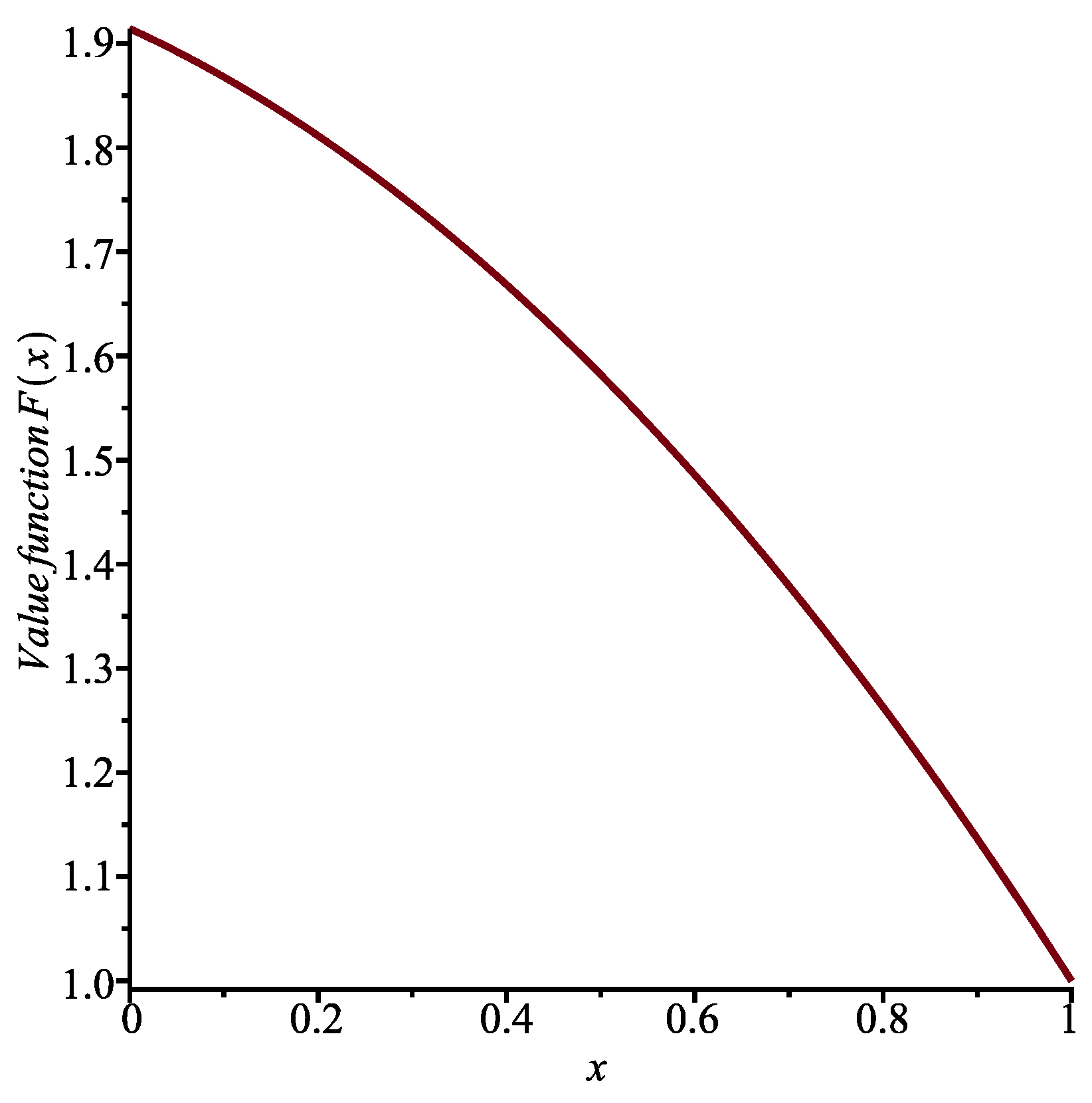
Let us take $\theta =\lambda =b_0=q_0=K_0=d=1$. The solution to the above first-order non-linear ordinary differential equation (ODE) that satisfies the boundary condition $F\left(1\right)=K_0=1$ is (see Figure 1)

$$F\left(x\right)=-{\displaystyle \frac{x^2}{2}}+(1-\sqrt{2}x)+\sqrt{2}+{\displaystyle \frac{1}{2}}\mathrm{for}0\le x\le 1.$$

(32)

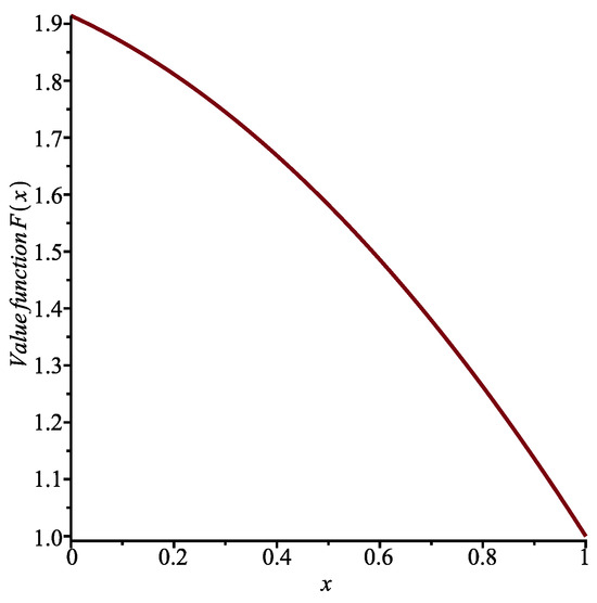
Figure 1. Value function $F\left(x\right)$ for $0\le x\le 1$ in Case I with $\theta =\lambda =b_0=q_0=K_0=d=1$.

Remark 3.

There is a second solution to Equation (31) that is such that $F\left(1\right)=1$, namely

$$F\left(x\right)=-{\displaystyle \frac{x^2}{2}}+(1+\sqrt{2}x)-\sqrt{2}+{\displaystyle \frac{1}{2}}\mathrm{for}0\le x\le 1.$$

(33)

However, because θ is positive, the value function $F\left(x\right)$ must also be positive in the interval $[0,1]$, as well as decreasing with increasing x. The function in the above equation is increasing and negative for $x\in [0,\sqrt{2}-1)$. Therefore, it must be discarded.

The optimal control is an affine function:

$$u^{*}\left(x\right)=x+\sqrt{2}-1\mathrm{for}0\le x\le 1.$$

(34)

Case II. Suppose that, in the previous case, the terminal cost function $K(·)$ is rather $K\left[X\right(\tau \left(x\right)\left)\right]=X\left(\tau \right(x\left)\right)$. It follows that

$${\int }_{-\infty }^{\infty }F(x+y)f_Y\left(y\right)\mathrm{d}y=F(x+c)=x+c.$$

(35)

We must now solve

$$0=-{\displaystyle \frac{1}{2}}{\displaystyle \frac{b_0^2}{q_0}}{\left[F^{\prime }\left(x\right)\right]}^2+\theta +\lambda (x+c)-\lambda F\left(x\right).$$

(36)

Choosing the same constants as those in Case I and $c=2$, the mathematical software program Maple finds that the solution to the above equation is

$$F\left(x\right)=3-{\displaystyle \frac{1}{2}}{\left[\mathrm{LambertW}\left(c_{1}exp\{-x-1\}\right)+1\right]}^2+x,$$

(37)

where $c_1$ is an arbitrary constant and LambertW is a special function defined in such a way that

$$\mathrm{LambertW}\left(x\right)e^{\mathrm{LambertW}\left(x\right)}=x.$$

(38)

Solving Equation (36) with the software program Mathematica yields an equivalent expression in terms of the ProductLog function, which gives the principal solution for w in the equation $z=w{e}^w$. However, both software programs fail to give the solution that satisfies the boundary condition $F\left(1\right)=1$, together with the other conditions in our problem: $F\left(x\right)$ must be positive and decreasing with $x\in [0,1]$.

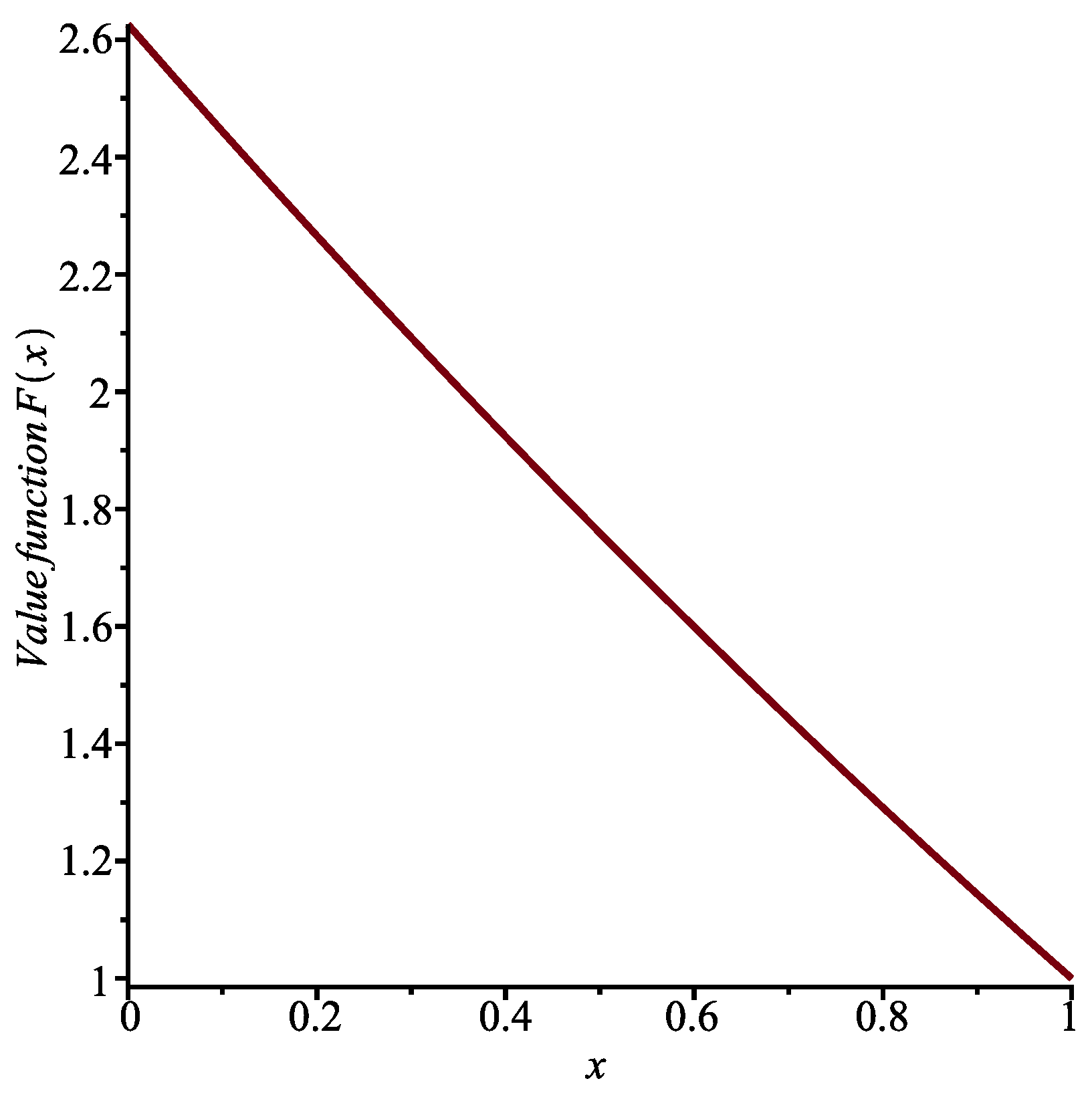
Making use of the NDSolve function in Mathematica, which employs a numerical technique, we obtain the graph shown in Figure 2. The solution that we are looking for is represented by the full line. From this function, we can determine the optimal control $u^{*}\left(x\right)$.

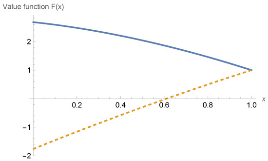
Figure 2. Value function $F\left(x\right)$ for $0\le x\le 1$ in Case II (full line) with $\theta =\lambda =b_0=q_0=K_0=d=1$ and $c=2$.

Remark 4.

Maple and Mathematica can solve (simple) integral equations, but not integro-differential equations directly. This is the reason why we must try to transform the equation into a (non-linear) ordinary differential equation. There are, however, many papers on numerical solutions of integro-differential equations; see, for example, [15].

Case III. Next, we assume that $Y\sim$ Exp$\left(\alpha \right)$, so that

$$f_Y\left(y\right)=\alpha e^{-\alpha y}\mathrm{for}y\ge 0.$$

(39)

We then have

$${\int }_{-\infty }^{\infty }F(x+y)f_Y\left(y\right)\mathrm{d}y={\int }_0^{d-x}F(x+y)\alpha e^{-\alpha y}\mathrm{d}y+{\int }_{d-x}^{\infty }K(x+y)\alpha e^{-\alpha y}\mathrm{d}y.$$

(40)

(a) First, we take $K\left(x\right)=K_0$ for $x\ge d$, as those in Case I. It follows that

$${\int }_{d-x}^{\infty }K(x+y)\alpha e^{-\alpha y}\mathrm{d}y=K_0{e}^{-\alpha (d-x)}.$$

(41)

Moreover, we can write that

$$I\left(x\right):={\int }_0^{d-x}F(x+y)\alpha e^{-\alpha y}\mathrm{d}y={\int }_x^{d}F\left(z\right)\alpha e^{-\alpha (z-x)}\mathrm{d}z.$$

(42)

We must solve the IDE

$$0=-{\displaystyle \frac{1}{2}}{\displaystyle \frac{b_0^2}{q_0}}{\left[F^{\prime }\left(x\right)\right]}^2+\theta -\lambda F\left(x\right)+\lambda \left\{I\left(x\right)+K_0{e}^{-\alpha (d-x)}\right\}.$$

(43)

We calculate

$$I^{\prime }\left(x\right)=\alpha [I\left(x\right)-F\left(x\right)].$$

(44)

Hence, differentiating Equation (43) with respect to x, we find that $F\left(x\right)$ satisfies the second-order non-linear ODE

$$0=-{\displaystyle \frac{b_0^2}{q_0}}{F}^{\prime }\left(x\right)F^{″}\left(x\right)-\lambda F^{\prime }\left(x\right)+{\displaystyle \frac{1}{2}}\alpha {\displaystyle \frac{b_0^2}{q_0}}{\left[F^{\prime }\left(x\right)\right]}^2-\alpha \theta .$$

(45)

This equation is subject to the boundary condition $F\left(d\right)=K_0$. Furthermore, we deduce from Equation (43) (and the fact that $F^{\prime }\left(x\right)$ must be negative) that

$$F^{\prime }\left(d\right)=-{\displaystyle \frac{\sqrt{2\theta q_0}}{b_0}}.$$

(46)

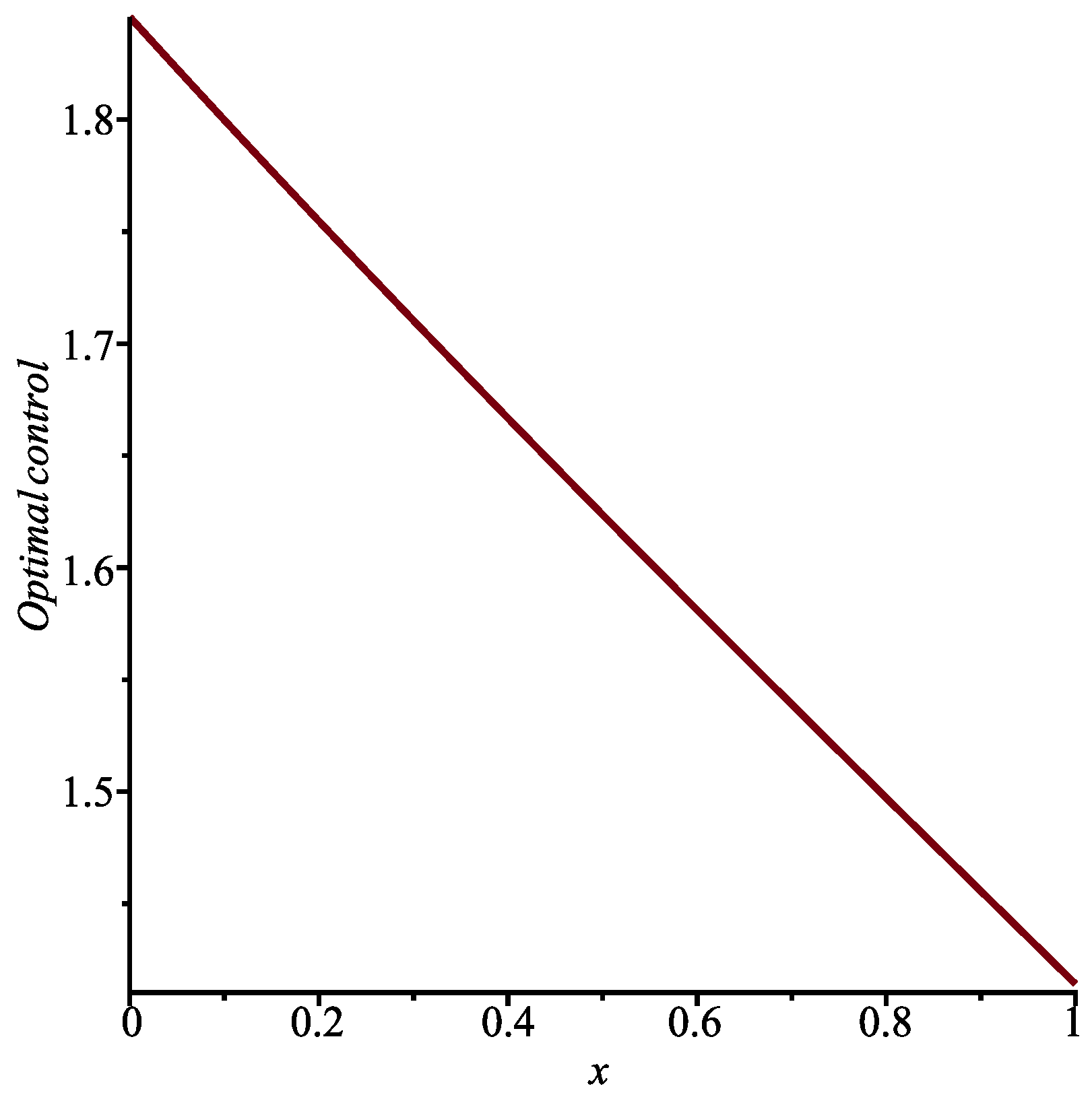
Choosing the same constants as those in Case I and $\alpha =1$, we can obtain (using a numerical method) both the value function $F\left(x\right)$ and the optimal control $u^{*}\left(x\right)$ in the interval $[0,1]$; see Figure 3 and Figure 4.

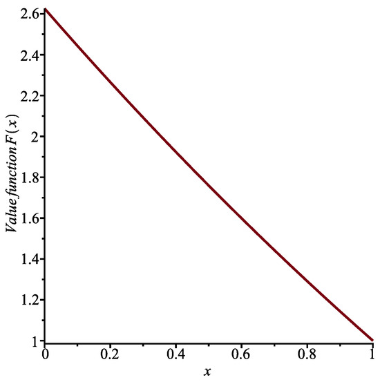
Figure 3. Value function $F\left(x\right)$ for $0\le x\le 1$ in Case III (a) with $\theta =\lambda =\alpha =b_0=q_0=K_0=d=1$.

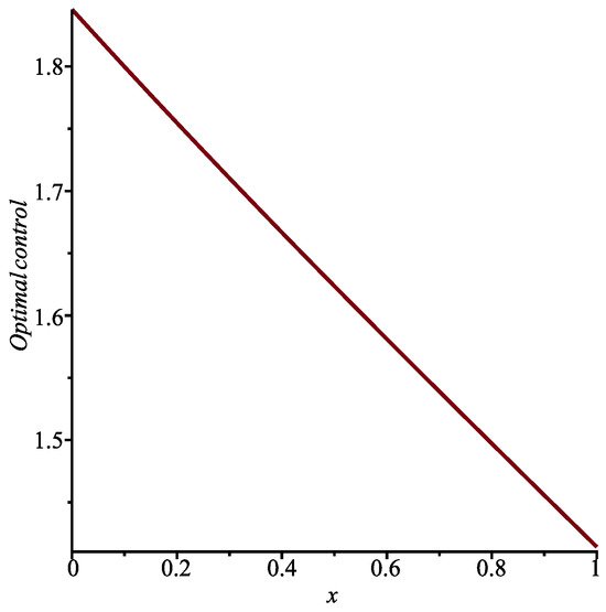
Figure 4. Optimal control for $0\le x\le 1$ in Case III (a) with $\theta =\lambda =\alpha =b_0=q_0=K_0=d=1$.

(b) If $K\left(x\right)=x$ for $x\ge d$, as in Case II, we calculate

$${\int }_{d-x}^{\infty }K(x+y)\alpha e^{-\alpha y}\mathrm{d}y={\displaystyle \frac{(\alpha d+1)}{{\alpha }^2}}{e}^{-\alpha (d-x)}.$$

(47)

It follows that the function $F\left(x\right)$ satisfies the IDE

$$0=-{\displaystyle \frac{1}{2}}{\displaystyle \frac{b_0^2}{q_0}}{\left[F^{\prime }\left(x\right)\right]}^2+\theta -\lambda F\left(x\right)+\lambda \left\{I\left(x\right)+{\displaystyle \frac{(\alpha d+1)}{{\alpha }^2}}{e}^{-\alpha (d-x)}\right\}.$$

(48)

Proceeding as in (a), we find that $F\left(x\right)$ satisfies Equation (45). However, the second boundary condition becomes

$$F^{\prime }\left(d\right)=-{\displaystyle \frac{\sqrt{2q_0}}{b_0}}\left(\theta -\lambda d+{\displaystyle \frac{\lambda (\alpha d+1)}{{\alpha }^2}}\right).$$

(49)

Hence, with the above constants, we now obtain that $F^{\prime }\left(1\right)=-2\sqrt{2}$.

Case IV. Finally, we suppose that $Y\sim$ U$[0,\alpha ]$, with $\alpha \le d$. We have

$${\int }_{-\infty }^{\infty }F(x+y)f_Y\left(y\right)\mathrm{d}y=\left\{\begin{array}{cc}{\displaystyle \frac{1}{\alpha }}{\int }_0^{\alpha }F(x+y)\mathrm{d}y& \mathrm{if}x+\alpha <d,\hfill \\ {\displaystyle \frac{1}{\alpha }}{\int }_0^{d-x}F(x+y)\mathrm{d}y+{\displaystyle \frac{1}{\alpha }}{\int }_{d-x}^{\alpha }K(x+y)\mathrm{d}y& \mathrm{if}x+\alpha \ge d.\hfill \end{array}\right.$$

(50)

(i) When $x+\alpha <d$, we must solve the IDE

$$\begin{array}{ccc}\hfill 0& =& -{\displaystyle \frac{1}{2}}{\displaystyle \frac{b_0^2}{q_0}}{\left[F^{\prime }\left(x\right)\right]}^2+\theta +{\displaystyle \frac{\lambda }{\alpha }}{\int }_0^{\alpha }F(x+y)\mathrm{d}y-\lambda F\left(x\right)\hfill \\ & =& -{\displaystyle \frac{1}{2}}{\displaystyle \frac{b_0^2}{q_0}}{\left[F^{\prime }\left(x\right)\right]}^2+\theta +{\displaystyle \frac{\lambda }{\alpha }}{\int }_x^{x+\alpha }F\left(z\right)\mathrm{d}z-\lambda F\left(x\right).\hfill \end{array}$$

(51)

It follows that $F\left(x\right)$ satisfies the equation

$$0=-{\displaystyle \frac{b_0^2}{q_0}}{F}^{\prime }\left(x\right)F^{″}\left(x\right)+{\displaystyle \frac{\lambda }{\alpha }}[F(x+\alpha )-F\left(x\right)]-\lambda F^{\prime }\left(x\right).$$

(52)

Now, we can write that

$$F(x+\alpha )-F\left(x\right)=\alpha F^{\prime }\left(x\right)+{\displaystyle \frac{{\alpha }^2}{2}}{F}^{″}\left(x\right)+\cdots ,$$

(53)

so that, if $\alpha$ is small,

$$0\approx -{\displaystyle \frac{b_0^2}{q_0}}{F}^{\prime }\left(x\right)F^{″}\left(x\right)+{\displaystyle \frac{\lambda \alpha }{2}}{F}^{″}\left(x\right).$$

(54)

Assuming that $F^{″}\left(x\right)\ne 0$, we thus have

$$F^{\prime }\left(x\right)\approx -{\displaystyle \frac{q_0}{b_0^2}}{\displaystyle \frac{\lambda \alpha }{2}}⟹F\left(x\right)\approx -{\displaystyle \frac{q_0}{b_0^2}}{\displaystyle \frac{\lambda \alpha }{2}}x+c_0,$$

(55)

where $c_0$ is an arbitrary constant.

(ii) In the case when $x+\alpha \ge d$, the IDE becomes

$$\begin{array}{ccc}\hfill 0& =& -{\displaystyle \frac{1}{2}}{\displaystyle \frac{b_0^2}{q_0}}{\left[F^{\prime }\left(x\right)\right]}^2+\theta +\lambda \left\{{\displaystyle \frac{1}{\alpha }}{\int }_0^{d-x}F(x+y)\mathrm{d}y+{\displaystyle \frac{1}{\alpha }}{\int }_{d-x}^{\alpha }K(x+y)\mathrm{d}y\right\}-\lambda F\left(x\right)\hfill \\ & =& -{\displaystyle \frac{1}{2}}{\displaystyle \frac{b_0^2}{q_0}}{\left[F^{\prime }\left(x\right)\right]}^2+\theta +\lambda \left\{{\displaystyle \frac{1}{\alpha }}{\int }_x^{d}F\left(z\right)\mathrm{d}z+{\displaystyle \frac{1}{\alpha }}{\int }_d^{x+\alpha }K\left(z\right)\mathrm{d}z\right\}-\lambda F\left(x\right).\hfill \end{array}$$

(56)

Differentiating with respect to x, we have

$$0=-{\displaystyle \frac{b_0^2}{q_0}}{F}^{\prime }\left(x\right)F^{″}\left(x\right)-{\displaystyle \frac{\lambda }{\alpha }}F\left(x\right)+{\displaystyle \frac{\lambda }{\alpha }}K(x+\alpha )-\lambda F^{\prime }\left(x\right).$$

(57)

To obtain an approximate expression for the function $F\left(x\right)$, we can first try to solve the above ODE, subject to the condition $F\left(d\right)=K\left(d\right)$ and the value of $F^{\prime }\left(d\right)$ deduced from Equation (56). Next, we can use the continuity of $F\left(x\right)$ to determine the value of the constant $c_0$ in Equation (55).

The Inverse Problem

As we have seen above, finding the value function $F\left(x\right)$ for a given density function $f_Y\left(y\right)$ is generally a difficult task. To end this paper, we will consider the inverse problem: if we assume that $F\left(x\right)$ is of a certain form, is there at least one density function $f_Y\left(y\right)$ (and a terminal cost function K) for which the function $F\left(x\right)$ can indeed be considered as the value function in a particular case of our homing problem?

Case I. The simplest case is of course the one when $F\left(x\right)$ is a positive constant $F_0$. Moreover, we assume that $K\left(x\right)\equiv F_0$ as well. Then, Equation (29) reduces to

$$0=\theta .$$

(58)

Hence, we deduce that $F\left(x\right)$ cannot be a constant, unless $\theta =0$. The corresponding optimal control would be identical to 0. This result is in fact obvious, because if $\theta =0$ and $K\left(x\right)\equiv F_0$, it is clear that $E\left[J\right(x\left)\right]$ cannot be smaller than $F_0$, which is obtained by choosing $u\left(x\right)\equiv 0$. Furthermore, as we mentioned earlier, the value function $F\left(x\right)$ should be decreasing as x increases when $\theta >0$, and therefore should not be a constant.

Suppose however that we replace the parameter $\theta$ in the cost function $J\left(x\right)$ by $\theta g\left[X\right(t\left)\right]$. The IDE (29) will then become

$$0=-{\displaystyle \frac{1}{2}}{\displaystyle \frac{b_0^2}{q_0}}{\left[F^{\prime }\left(x\right)\right]}^2+\theta g\left(x\right)+\lambda {\int }_{-\infty }^{\infty }F(x+y)f_Y\left(y\right)\mathrm{d}y-\lambda F\left(x\right).$$

(59)

Assume that $x\ge 0$ and that $K\left(x\right)=F_{0}x/d$ (so that $K\left(d\right)=F\left(d\right)=F_0$, as required). Then, if $Y\sim$ U$[0,d]$, we obtain the equation

$$\begin{array}{ccc}\hfill 0& =& \theta g\left(x\right)+\lambda \left\{F_{0}P[Y<d-x]+{\int }_{d-x}^{\infty }K(x+y)f_Y\left(y\right)\mathrm{d}y\right\}-\lambda F_0\hfill \\ & =& \theta g\left(x\right)-\lambda F_{0}P[Y\ge d-x]+{\displaystyle \frac{\lambda }{d}}{\int }_{d-x}^{d}K(x+y)\mathrm{d}y\hfill \\ & =& \theta g\left(x\right)-{\displaystyle \frac{\lambda F_0}{d}}x+{\displaystyle \frac{\lambda F_0}{d^2}}{\int }_{d-x}^d(x+y)\mathrm{d}y\hfill \\ & =& \theta g\left(x\right)+{\displaystyle \frac{\lambda F_0}{2d^2}}{x}^2.\hfill \end{array}$$

(60)

Thus, the value function will indeed be equal to the constant $F_0$ (and $u^{*}\left(x\right)\equiv 0$) if and only if

$$g\left(x\right)=-{\displaystyle \frac{\lambda F_0}{2\theta d^2}}{x}^2.$$

(61)

Note that the aim would be to keep the controlled process in the interval $[0,d)$ for as long as possible (taking into account the quadratic control costs), rather than trying to minimize the expected time spent by the process in $[0,d)$.

Case II. Next, we look for value functions of the form $F\left(x\right)=F_{1}x+F_0$ for $x\in [0,d]$, where $F_1<0$ and $F_0\ge -F_{1}d$, and we assume that $K\left(x\right)=F\left(x\right)$. Substituting the expression for $F\left(x\right)$ and $K\left(x\right)$ into the IDE (29), we obtain, after simplification, that we must have

$$0=\theta -{\displaystyle \frac{1}{2}}{\displaystyle \frac{b_0^2}{q_0}}{F}_1^2+\lambda F_{1}E\left[Y\right].$$

(62)

It follows that this solution is valid for any (positive) random variable Y having an expected value $E\left[Y\right]$ such that

$$F_1=\lambda \kappa E\left[Y\right]-\sqrt{{\left(\lambda \kappa E\left[Y\right]\right)}^2+2\kappa \theta },$$

(63)

where $\kappa :=q_0/b_0^2$. The optimal control would be $u^{*}\left(x\right)\equiv -b_0{F}_1/q_0>0$.

This case could be generalized by taking $K\left(x\right)=K_{1}x+K_0$, with $F_{1}d+F_0=K_{1}d+K_0$.

4. Discussion

In this paper, a homing problem for FPPs was set up and solved explicitly in various particular cases. This is the first time such problems were considered for FPPs. These processes have applications in numerous fields. Therefore, the results that we obtained may be useful for people working in these fields.

To obtain exact solutions to our problem, we had to solve a non-linear integro-differential equation, which is the main limitation of the technique used in this paper. Sometimes, this equation can be transformed into a differential equation. However, solving this differential equation, subject to the appropriate boundary conditions, is in itself a difficult problem.

We can at least try to find approximate analytical expressions for the value function and the optimal control. When this is not possible, we can resort to numerical methods or simulation.

A possible extension of the work presented in this paper would be to treat the case when the parameter $\theta$ in the cost function $J\left(x\right)$ is negative, so that there is a reward as long as the controlled process is in the continuation region. As mentioned above, in the application of the FPPs in hydrology, the problem could be to maintain the level of a river below a critical value for as long as possible, beyond which the risk of flooding is high. We could also add some noise in the form of a diffusion process to the model. Having time-varying parameters is another possibility. However, then the equation satisfied by the value function would include a partial derivative with respect to time, making the task of finding an explicit solution to this equation even more challenging.

References

- Parzen, E. Stochastic Processes; Holden-Day: San Francisco, CA, USA, 1962. [Google Scholar]
- Lefebvre, M.; Guilbault, J.-L. Using filtered Poisson processes to model a river flow. Appl. Math. Model. 2008, 32, 2792–2805. [Google Scholar] [CrossRef]
- Racicot, R.W.; Moses, F. Filtered Poisson process for random vibration problems. J. Eng. Mech. Div. 1972, 98, 159–176. [Google Scholar] [CrossRef]
- Hero, A.O. Timing estimation for a filtered Poisson process in Gaussian noise. IEEE Trans. Inf. Theory 1991, 37, 92–106. [Google Scholar] [CrossRef]
- Grigoriu, M. Dynamic systems with Poisson white noise. Nonlinear Dyn. 2004, 36, 255–266. [Google Scholar] [CrossRef]
- Novikov, A.; Melchers, R.E.; Shinjikashvili, E.; Kordzakhia, N. First passage time of filtered Poisson process with exponential shape function. Probabilist. Eng. Mech. 2005, 20, 57–65. [Google Scholar] [CrossRef]
- Yin, Y.-J.; Li, Y.; Bulleit, W.M. Stochastic modeling of snow loads using a filtered Poisson process. J. Cold Reg. Eng. 2011, 25, 16–36. [Google Scholar] [CrossRef]
- Theodorsen, A.; Garcia, O.E.; Rypdal, M. Statistical properties of a filtered Poisson process with additive random noise: Distributions, correlations and moment estimation. Phys. Scr. 2017, 92, 054002. [Google Scholar] [CrossRef]
- Alazemi, F.; Khalifa Es-Sebaiy, K.; Ouknine, Y. Efficient and superefficient estimators of filtered Poisson process intensities. Commun. Stat. Theory Methods 2019, 48, 1682–1692. [Google Scholar] [CrossRef]
- Grant, J.A.; Szechtman, R. Filtered Poisson process bandit on a continuum. Eur. J. Oper. Res. 2021, 295, 575–586. [Google Scholar] [CrossRef]
- Whittle, P. Optimization over Time; Wiley: Chichester, UK, 1982; Volume I. [Google Scholar]
- Whittle, P. Risk-Sensitive Optimal Control; Wiley: Chichester, UK, 1990. [Google Scholar]
- Lefebvre, M.; Yaghoubi, R. Optimal service time distribution for an M/G/1 queue. Axioms 2024, 13, 594. [Google Scholar] [CrossRef]
- Bellman, R. Dynamic Programming; Princeton University Press: Princeton, NJ, USA, 1957. [Google Scholar]
- Mohammed, J.K.; Khudair, A.R. Integro-differential equations: Numerical solution by a new operational matrix based on fourth-order hat functions. Partial Differ. Equ. Appl. Math. 2023, 8, 100529. [Google Scholar] [CrossRef]
Disclaimer/Publisher’s Note: The statements, opinions and data contained in all publications are solely those of the individual author(s) and contributor(s) and not of MDPI and/or the editor(s). MDPI and/or the editor(s) disclaim responsibility for any injury to people or property resulting from any ideas, methods, instructions or products referred to in the content. |
© 2025 by the author. Licensee MDPI, Basel, Switzerland. This article is an open access article distributed under the terms and conditions of the Creative Commons Attribution (CC BY) license (https://creativecommons.org/licenses/by/4.0/).