Application of Natural Generalized-Laplace Transform and Its Properties

Abstract

In this work, we combine the Natural Transform and generalized-Laplace Transform into a new transform called, the Natural Generalized-Laplace Transform, (NGLT) and some of its properties are provided. Moreover, the existence condition, convolution theorem, periodic theorem, and non-constant coefficient partial derivatives are proved with some details. The (NGLT) is applied to gain the solutions of linear telegraph and partial integro-differential equations. Also, we obtained the solution of the singular one-dimensional Boussinesq equation by employing the Natural Generalized-Laplace Transform Decomposition Method, (NGLTDM).

1. Introduction

Partial differential equations (PDEs) play a fundamental role across numerous disciplines, including physics, engineering, and the broader sciences. In recent years, there has been growing scholarly interest in developing analytical techniques for solving both ordinary differential equations (ODEs) and PDEs, driven by the need for precise and efficient models of complex phenomena; for example, in [1], the authors addressed the solution of both linear and nonlinear integro-differential equations defined on arbitrary time scales by employing the Laplace-Adomian Decomposition Method (LADM). In [2], the authors employed both the classical Adomian Decomposition Method (ADM) and its improved variant (IADM) to investigate the computational significance of the GI equation in modeling shock wave phenomena, using a benchmark exact soliton solution for validation. In [3], the authors employed the Sumudu Transform Adomian Decomposition Method (STADM) to obtain solutions to the n-generalized Korteweg–de Vries (KdV) equation within the framework of fractional calculus. In [4], the authors derived solutions to the telegraph equation and a class of partial integro-differential equations by employing the Double Laplace Transform technique. In [5], the Double Laplace Transform was employed to obtain solutions for the heat, wave, and Laplace equations involving convolution terms. In [6] the authors used the finite integral transform method to derive exact bending solutions for fully clamped orthotropic rectangular thin plates subjected to arbitrary loading conditions. Natural Transform was first obtained by [7], and later its properties were discussed by [8,9]. The Natural Decomposition Method was used to solve a coupled system of nonlinear PDEs; see [10]. In [11] the authors successfully applied the Natural Homotopy Perturbation Method to obtain analytical solutions for both linear and nonlinear Schrödinger equations. In [12], the researchers extended the concept of the one-dimensional Natural Transform to a two-dimensional framework, referred to as the Double Natural Transform. This generalized approach was subsequently applied to derive solutions for linear telegraph equations, wave equations, and partial integro-differential equations. The Natural Transform Decomposition Method (NTDM) has proven to be an effective analytical tool for deriving solutions to partial differential equations [13,14]. Linear and nonlinear Boussinesq equations serve as mathematical models for a wide range of scientific, engineering, and technological processes, including the simulation of water flow in unconfined aquifers. To construct both general and periodic solutions to the Boussinesq equation, researchers have employed the Modified Decomposition Method as an effective analytical approach in [15,16]. This study proposes analytical solutions for non-homogeneous telegraphic equation, partial integro-differential equations and the singular one-dimensional Boussinesq equation by employing the Natural Generalized-Laplace Transform (NGLT), and the Natural Generalized-Laplace Transform Decomposition Method (NGLTDM), respectively. This analytical technique examines how the solutions of the differential equations can be approximated.

Remark 1.

Throughout this study, we adopt the following abbreviations:

• (1) (GLT) instead of ”Generalized-Laplace Transform”.
• (2) (NT) instead of ” Natural transform”.
• (3) (NGLT) instead of ” Natural Generalized-Laplace Transform”.
• (4) (INGLT) instead of ” Inverse Natural Generalized-Laplace Transform”.
• (5) (NGLTDM) instead of ” Natural Generalized-Laplace Transform Decomposition Method”.

Let us recall the definitions of the Natural Transform (NT) and Generalized-Laplace Transform (GLT), respectively.

Definition 1.

Over the set of functions

$$A=\left\{\begin{array}{c}f\left(x\right):\exists M,{\tau }_1,{\tau }_2>0,\mathit{such}\mathit{that}\\ \left|f\left(x\right)\right|<M{e}^{{\displaystyle \frac{\left|x\right|}{{\tau }_j}}},,\mathit{if}t\in {(-1)}^j\times [0,\infty ),j=1,2.\end{array}\right\}$$

the Natural Transform (NT) is defined by

$${\mathbf{N}}_x^{+}\left[f\left(t\right)\right]=R\left(p;u\right)={\displaystyle \frac{1}{u}}{\int }_0^{\infty }{e}^{-{\displaystyle \frac{p}{u}}x}f\left(x\right)dx,\mathrm{Re}\left(p\right),\mathrm{Re}\left(u\right)>0,$$

(1)

where the variables u and p are complex variables of the (NT); for more details we refer to [7,8].

Definition 2

([17]). Let $f\left(t\right)$ be an integrable function, for all $t\ge 0$. The Generalized-Laplace Transform $G_{\alpha }$ of the function $f\left(t\right)$ is given by

$$F\left(s\right)=G_{\alpha }\left(f\right)=s^{\alpha }{\displaystyle \underset{0}{\overset{\infty }{\int }}}f\left(t\right)e^{-{\displaystyle \frac{t}{s}}}d\nu ,$$

(2)

for, $s\in \mathbb{C}$ and $\alpha \in Z$.

In the following sections, we address the main results of this work.

2. Properties of Natural Generalized-Laplace Transform

Here we explain the basic ideas and properties of the (NGLT) utilized in the consequence.

$$\begin{array}{ccc}\hfill {\mathbf{N}}_x^{+}{G}_t\left[f\left(x,t\right)\right]& =& F\left(p;u,s\right)={\displaystyle \frac{s^{\alpha }}{u}}{\int }_0^{\infty }{\int }_0^{\infty }{e}^{-{\displaystyle \frac{p}{u}}x-{\displaystyle \frac{1}{s}}t}f(x,t)dtdx,\hfill \\ \hfill \mathrm{Re}\left(s\right),\mathrm{Re}\left(p\right)& >& 0,\mathrm{Re}\left(u\right)>0\mathrm{and}\alpha \in Z,\hfill \end{array}$$

(3)

where ${\mathbf{N}}_x^{+}{G}_t$ denotes the (NGLT). The inverse Natural Generalized-Laplace Transform (INGLT) is described by

$${\mathbf{N}}_{p;u}^{-1}{G}_s^{-1}\left(F\left(p;u,s\right)\right)=f\left(x,t\right)={\displaystyle \frac{1}{{\left(2\pi i\right)}^2}}{\int }_{\lambda -i\infty }^{\lambda -i\infty }{\int }_{\beta -i\infty }^{\beta -i\infty }{e}^{{\displaystyle \frac{p}{u}}x+{\displaystyle \frac{1}{s}}t}F\left(p;u,s\right)dsdp.$$

Remark 2.

From the definition of (NGLT), we generate the following transformation:

1. 

Setting $\alpha =-1, p=1$ and $s=v$, we gained double Sumudu transform

$${\mathbf{S}}_x{S}_t\left[f\left(x,t\right)\right]=F\left(u,v\right)={\displaystyle \frac{1}{uv}}{\int }_0^{\infty }{\int }_0^{\infty }{e}^{-{\displaystyle \frac{1}{u}}x-{\displaystyle \frac{1}{v}}t}f(x,t)dtdx,$$

2. 

Setting $\alpha =0, u=1$ and $s={\displaystyle \frac{1}{s}},$ we obtained Double Laplace Transform as

$$L_x{L}_t\left[f\left(x,t\right)\right]=F\left(p,s\right)={\int }_0^{\infty }{\int }_0^{\infty }{e}^{-px-st}f(x,t)dtdx,$$

3. 

Setting $\alpha =0, u=1$ and $s=\omega ,$ we obtained Laplace–Yang Transform

$$L_{x}Y\left[f\left(x,t\right)\right]=F\left(p,\omega \right)={\int }_0^{\infty }{\int }_0^{\infty }{e}^{-px-{\displaystyle \frac{1}{\omega }}t}f(x,t)dtdx,$$

The next examples are useful in this paper.

Example 1.

The (NGLT) of the function $f(x,t)=e^{ax+bt}$ is granted by

$$F\left(p;u,s\right)={\mathbf{N}}_x^{+}{G}_t\left[e^{ax+bt}\right]={\displaystyle \frac{1}{\left(p-au\right)}}{\displaystyle \frac{s^{\alpha +1}}{\left(1-bs\right)}}$$

Example 2.

The (NGLT) of $f(x,t)={\left(xt\right)}^n$ is denoted by

$${\mathbf{N}}_x^{+}{G}_t\left[{\left(xt\right)}^n\right]={\displaystyle \frac{{\left(n!\right)}^2{u}^n{s}^{n+\alpha +1}}{p^{n+1}}},$$

where n is a positive integer. If $a(>-1)$ and $b(>-1)$ are real numbers, then

$${\mathbf{N}}_x^{+}{G}_t\left[x^a{t}^b\right]={\displaystyle \frac{u^a\Gamma \left(a+1\right)\Gamma \left(b+1\right)s^{\alpha +b+1}}{p^{a+1}}},$$

then it follows from the definition of (NGLT) that

$$\begin{array}{ccc}{\mathbf{N}}_x^{+}{G}_t\left[x^a{t}^b\right]& =& {\displaystyle \frac{s^{\alpha }}{u}}{\int }_0^{\infty }{\int }_0^{\infty }{e}^{-{\displaystyle \frac{p}{u}}x-{\displaystyle \frac{s}{v}}t}{x}^a{t}^{b}dtdx\\ & =& {\displaystyle \frac{1}{u}}{\int }_0^{\infty }{e}^{-{\displaystyle \frac{p}{u}}x}{x}^a\left(s^{\alpha }{\int }_0^{\infty }{e}^{-{\displaystyle \frac{1}{s}}t}{t}^{b}dt\right)dx,\hfill \end{array}$$

by substituting ${\displaystyle \frac{p}{u}}x=r$, and ${\displaystyle \frac{1}{s}}t=q,$ one gets

$$\begin{array}{ccc}{\mathbf{N}}_x^{+}{G}_t\left[x^a{t}^b\right]& =& {\displaystyle \frac{1}{u}}{\int }_0^{\infty }{\left({\displaystyle \frac{u}{p}}r\right)}^a{e}^{-r}{\displaystyle \frac{u}{p}}dr{s}^{\alpha }{\int }_0^{\infty }{\left(sq\right)}^b{e}^{-q}sdq\hfill \\ & =& {\displaystyle \frac{u^a}{p^{a+1}}}{s}^{\alpha +b+1}{\int }_0^{\infty }{\int }_0^{\infty }{r}^a{q}^b{e}^{-r}{e}^{-q}drdq\\ & =& {\displaystyle \frac{u^a\Gamma \left(a+1\right)\Gamma \left(b+1\right)s^{\alpha +b+1}}{p^{a+1}}},\end{array}$$

where gamma functions of a and b are defined by the uniformly convergent integral as follows.

$$\Gamma \left(a\right)\Gamma \left(b\right)={\int }_0^{\infty }{e}^{-r}{r}^{a-1}dx{\int }_0^{\infty }{e}^{-q}{q}^{b-1}dt,,a>0,b>0.$$

• Existence Condition for the (NGLT):

If $f(x,t)$ is an exponential order c and d as $x\to \infty$, $t\to \infty ,$ if there exists a positive constant M such that for all $x>X$ and $t>T$

$$\left|f(x,t)\right|\le M{e}^{cx+dt},$$

(4)

it is straightforward to gain,

$$f(x,t)=O\left(e^{cx+dt}\right)\mathrm{as}x\to \infty ,t\to \infty ,$$

Or equally,

$$\underset{\begin{array}{c}x\to \infty \\ t\to \infty \end{array}}{\lim }{e}^{-{\displaystyle \frac{\mu }{u}}x-{\displaystyle \frac{1}{\nu }}t}\left|f(x,t)\right|=K\underset{\begin{array}{c}x\to \infty \\ t\to \infty \end{array}}{\lim }{e}^{-\left({\displaystyle \frac{\mu }{u}}-c\right)x-\left({\displaystyle \frac{1}{\nu }}-d\right)t}=0,$$

where ${\displaystyle \frac{\mu }{u}}>c$ and ${\displaystyle \frac{1}{\nu }}>d.$ The function $f(x,t)$ is named an exponential order as $x\to \infty ,t\to \infty$, and obviously, it does not grow faster than ${Me}^{cx+dt}$ as $x\to \infty ,t\to \infty$.

Theorem 1.

If a function $f(x,t)$ is continuous in every bounded interval $(0,X)$ and $(0,T)$ and of exponential order $e^{cx+dt}$, then the (NGLT) of $f(x,t)$, which is determined by $F\left(p;u,s\right)$, exists $\forall \mathrm{Re}{\displaystyle \frac{p}{u}}>c,\forall \mathrm{Re}{\displaystyle \frac{1}{s}}>d$.

Proof. 

Applying the definition of (NGLT) for the $f(x,t),$ we have

$$\begin{array}{ccc}\left|F\left(p;u,\nu \right)\right|& =& \left|{\displaystyle \frac{{\nu }^{\alpha }}{u}}{\int }_0^{\infty }{\int }_0^{\infty }{e}^{-{\displaystyle \frac{p}{u}}x-{\displaystyle \frac{1}{\nu }}t}f(x,t)dtdx\right|\\ & \le & M\left|{\displaystyle \frac{v^{\alpha }}{u}}{\int }_0^{\infty }{\int }_0^{\infty }{e}^{-\left({\displaystyle \frac{p}{u}}-c\right)x-\left({\displaystyle \frac{1}{v}}-d\right)t}dtdx\right|\\ & =& {\displaystyle \frac{M{v}^{\alpha +1}}{\left(p-cu\right)\left(1-dv\right)}}.\end{array}$$

(5)

From Equation (5) we conclude

$$\underset{\begin{array}{c}x\to \infty \\ t\to \infty \end{array}}{\lim }\left|F\left(p;u,v\right)\right|=0\mathrm{or}\underset{\begin{array}{c}x\to \infty \\ t\to \infty \end{array}}{\lim }F\left(p;u,v\right)=0.$$

□

Theorem 2.

Assume that the (NGLT) of the function $f(x,t)$ exists and $f(x,t)$ is a periodic function of periods M and T where $f(x+M,t+T)=f(x,t),$$\forall \left(x,t\right)$, hence

$${\mathbf{N}}_x^{+}{G}_t\left[f\left(x,t\right)\right]={\displaystyle \frac{\frac{s^{\alpha }}{u}{\int }_0^T{\int }_0^M{e}^{-\frac{p}{u}x-\frac{1}{s}t}f\left(x,t\right)dtdx}{\left(1-\frac{s^{\alpha }}{u}{e}^{-\frac{p}{u}M-\frac{1}{s}T}\right)}}$$

Proof. 

By using definition of (NGLT), we have

$$\begin{array}{ccc}{\mathbf{N}}_x^{+}{G}_t\left[f\left(x,t\right)\right]& =& {\displaystyle \frac{s^{\alpha }}{u}}{\int }_0^{\infty }{\int }_0^{\infty }{e}^{-{\displaystyle \frac{p}{u}}x-{\displaystyle \frac{1}{s}}t}f\left(x,t\right)dtdx\\ & =& {\displaystyle \frac{s^{\alpha }}{u}}{\int }_0^T{\int }_0^M{e}^{-{\displaystyle \frac{p}{u}}x-{\displaystyle \frac{1}{s}}t}f\left(x,t\right)dtdx\\ & & +{\displaystyle \frac{s^{\alpha }}{u}}{\int }_T^{\infty }{\int }_M^{\infty }{e}^{-{\displaystyle \frac{p}{u}}x-{\displaystyle \frac{1}{s}}t}f\left(x,t\right)dtdx.\end{array}$$

Let $x=M+\rho$ and $t=T+\sigma ,$ the last integral in the R.H.S; thus we have

$$\begin{array}{ccc}{\mathbf{N}}_x^{+}{G}_t\left[f\left(x,t\right)\right]& =& {\displaystyle \frac{s^{\alpha }}{u}}{\int }_0^T{\int }_0^M{e}^{-{\displaystyle \frac{p}{u}}x-{\displaystyle \frac{1}{s}}t}f\left(x,t\right)dtdx\hfill \\ & & +{\displaystyle \frac{s^{\alpha }}{u}}{e}^{-{\displaystyle \frac{p}{u}}M-{\displaystyle \frac{1}{s}}T}{\int }_0^{\infty }{\int }_0^{\infty }{e}^{-{\displaystyle \frac{p}{u}}\rho -{\displaystyle \frac{1}{s}}\sigma }f\left(M+\rho ,T+\sigma \right)d\sigma d\rho ,\hfill \end{array}$$

by using the relation $f(x+M,t+T)=f(x,t),$ the above equation becomes

$$\begin{array}{ccc}{\mathbf{N}}_x^{+}{G}_t\left[f\left(x,t\right)\right]& =& {\displaystyle \frac{s^{\alpha }}{u}}{\int }_0^T{\int }_0^M{e}^{-{\displaystyle \frac{p}{u}}x-{\displaystyle \frac{1}{s}}t}f\left(x,t\right)dtdx\hfill \\ & & +{\displaystyle \frac{s^{\alpha }}{u}}{e}^{-{\displaystyle \frac{p}{u}}M-{\displaystyle \frac{1}{s}}T}{\int }_0^{\infty }{\int }_0^{\infty }{e}^{-{\displaystyle \frac{p}{u}}\rho -{\displaystyle \frac{1}{s}}\sigma }f\left(\rho ,\sigma \right)d\sigma d\rho ,\hfill \end{array}$$

hence

$$\begin{array}{ccc}{\mathbf{N}}_x^{+}{G}_t\left[f\left(x,t\right)\right]& =& {\displaystyle \frac{s^{\alpha }}{u}}{\int }_0^T{\int }_0^M{e}^{-{\displaystyle \frac{p}{u}}x-{\displaystyle \frac{1}{s}}t}f\left(x,t\right)dtdx\hfill \\ & & +{\displaystyle \frac{s^{\alpha }}{u}}{e}^{-{\displaystyle \frac{p}{u}}M-{\displaystyle \frac{1}{s}}T}{\mathbf{N}}_x^{+}{G}_t\left[f\left(x,t\right)\right],\hfill \end{array}$$

therefore

$${\mathbf{N}}_x^{+}{G}_t\left[f\left(x,t\right)\right]={\displaystyle \frac{\frac{s^{\alpha }}{u}{\int }_0^T{\int }_0^M{e}^{-\frac{p}{u}x-\frac{1}{s}t}f\left(x,t\right)dtdx}{\left(1-\frac{s^{\alpha }}{u}{e}^{-\frac{p}{u}M-\frac{1}{s}T}\right)}}.$$

□

• The Natural Transform of the convolution product:

Theorem 3.

The (NGLT) of the functions $f(x,t)$ and $g(x,t)$ exists. Then (NGLT) of the double convolution of the $f(x,t)$ and $g(x,t)$,

$$\left(f\ast \ast g\right)\left(x,t\right)={\int }_0^x{\int }_0^{t}f\left(x-\zeta ,t-\eta \right)g\left(\zeta ,\eta \right)d\eta d\zeta ,$$

(6)

specified by

$${\mathbf{N}}_x^{+}{G}_t\left[f\left(x,t\right)\ast \ast g\left(x,t\right)\right]={\displaystyle \frac{u}{s^{\alpha }}}F\left(p;u,s\right)G\left(p;u,s\right).$$

(7)

where $F\left(p;u,s\right)$ and $G\left(p;u,s\right)$ are the (NGLT) of the functions $f\left(x,t\right)$ and $g\left(x,t\right)$, respectively, and the variables $u,p$ and s are the complex variables of the (NGLT).

Proof. 

Utilizing the definition of the (NGLT) and double convolution yields that

$$\begin{array}{ccc}{\mathbf{N}}_x^{+}{G}_t\left[f\left(x,t\right)\ast \ast g\left(x,t\right)\right]& =& {\displaystyle \frac{s^{\alpha }}{u}}{\int }_0^{\infty }{\int }_0^{\infty }{e}^{-{\displaystyle \frac{p}{u}}x-{\displaystyle \frac{1}{s}}t}f\left(x,t\right)\ast \ast g\left(x,t\right)dtdx\hfill \\ & =& {\displaystyle \frac{s^{\alpha }}{u}}{\int }_0^{\infty }{\int }_0^{\infty }{e}^{-{\displaystyle \frac{p}{u}}x-{\displaystyle \frac{1}{s}}t}\left({\int }_0^x{\int }_0^{t}f\left(\zeta ,\eta \right)g\left(x-\zeta ,t-\eta \right)d\zeta d\eta \right)dtdx,\hfill \end{array}$$

putting $\gamma =x-\zeta$ and $\delta =t-\eta$ and stretching the upper boundaries of integrals to $x\to \infty$, $t\to \infty$ means that

$${\mathbf{N}}_x^{+}{G}_t\left[f\left(x,t\right)\ast \ast g\left(x,t\right)\right]={\displaystyle \frac{s^{\alpha }}{u}}{\int }_0^{\infty }{\int }_0^{\infty }{e}^{-{\displaystyle \frac{p}{u}}x-{\displaystyle \frac{1}{s}}t}f\left(\zeta ,\eta \right)\left({\int }_{-\gamma }^{\infty }{\int }_{-\delta }^{\infty }{e}^{-{\displaystyle \frac{p}{u}}\gamma -{\displaystyle \frac{1}{s}}\delta }g\left(\gamma ,\delta \right)d\gamma d\delta \right)d\zeta d\eta ,$$

where the functions $f\left(x,t\right)$, $g\left(x,t\right)$ are defined at $x>0,$ $t>0.$ Hence $f\left(x,t\right)$, $g\left(x,t\right)$ are zero at $x<0$, $t<0,$ therefore

$${\mathbf{N}}_x^{+}{G}_t\left[f\left(x,t\right)\ast \ast g\left(x,t\right)\right]={\displaystyle \frac{u}{s^{\alpha }}}\left({\displaystyle \frac{s^{\alpha }}{u}}{\int }_0^{\infty }{\int }_0^{\infty }{e}^{-{\displaystyle \frac{p}{u}}x-{\displaystyle \frac{1}{s}}t}f\left(\zeta ,\eta \right)\left({\displaystyle \frac{s^{\alpha }}{u}}{\int }_0^{\infty }{\int }_0^{\infty }{e}^{-{\displaystyle \frac{p}{u}}\gamma -{\displaystyle \frac{1}{s}}\delta }g\left(\gamma ,\delta \right)d\gamma d\delta \right)d\zeta d\eta \right),$$

Thus

$${\mathbf{N}}_x^{+}{G}_t\left[f\left(x,t\right)\ast \ast g\left(x,t\right)\right]={\displaystyle \frac{u}{s^{\alpha }}}F\left(p;u,s\right)G\left(p;u,s\right).$$

  □

• The fundamental properties of the (NGLT) of partial derivatives:

If the (NGLT) of the function $f(x,t)$ is given by ${\mathbf{N}}_x^{+}{G}_t\left[f\left(x,t\right)\right]=F\left(p;u,s\right)$ then the (NGLT) of ${\displaystyle \frac{\partial f\left(x,t\right)}{\partial x}},$${\displaystyle \frac{{\partial }^{2}f\left(x,t\right)}{\partial x^2}},$${\displaystyle \frac{\partial f\left(x,t\right)}{\partial t}}$ and ${\displaystyle \frac{{\partial }^{2}f\left(x,t\right)}{\partial t^2}}$ are granted by

$$\begin{array}{ccc}{\mathbf{N}}_x^{+}{G}_t\left[{\displaystyle \frac{\partial f\left(x,t\right)}{\partial x}}\right]& =& {\displaystyle \frac{p}{u}}F\left(p;u,s\right)-{\displaystyle \frac{1}{u}}f\left(0,s\right),\hfill \end{array}$$

(8)

$$\begin{array}{ccc}{\mathbf{N}}_x^{+}{G}_t\left[{\displaystyle \frac{{\partial }^{2}f\left(x,t\right)}{\partial x^2}}\right]& =& {\displaystyle \frac{p^2}{u^2}}F\left(p;u,s\right)-{\displaystyle \frac{p}{u^2}}f\left(0,s\right)-{\displaystyle \frac{1}{u}}{\displaystyle \frac{\partial f\left(0,s\right)}{\partial x}},\hfill \end{array}$$

(9)

and

$$\begin{array}{ccc}{\mathbf{N}}_x^{+}{G}_t\left[{\displaystyle \frac{\partial f\left(x,t\right)}{\partial t}}\right]& =& {\displaystyle \frac{F\left(p;u,s\right)}{s}}-s^{\alpha }f\left(p;u,0\right),\hfill \end{array}$$

(10)

$$\begin{array}{ccc}{\mathbf{N}}_x^{+}{G}_t\left[{\displaystyle \frac{{\partial }^{2}f\left(x,t\right)}{\partial t^2}}\right]& =& {\displaystyle \frac{F\left(p;u,s\right)}{s^2}}-s^{\alpha -1}f\left(p,0\right)-s^{\alpha }{\displaystyle \frac{\partial f\left(p,0\right)}{\partial t}},\hfill \end{array}$$

(11)

In the next theorem, we discuss the (NGLT) of the functions $xg\left(x,t\right)$, $x{\displaystyle \frac{\partial f\left(x,t\right)}{\partial t}}$ and $x{\displaystyle \frac{{\partial }^{2}f\left(x,t\right)}{\partial t^2}}$. The following theorem has two proofs: In the first proof, we apply the derivative with respect to p, and in the second proof employ the derivative with respect to u, as follows.

Theorem 4.

If the (NGLT) of the partial derivatives ${\displaystyle \frac{\partial f\left(x,t\right)}{\partial t}}$ and ${\displaystyle \frac{{\partial }^{2}f\left(x,t\right)}{\partial t^2}}$ are denoted by Equations (10) and (11), then the (NGLT) of the $x{\displaystyle \frac{\partial f\left(x,t\right)}{\partial t}}$, $x{\displaystyle \frac{{\partial }^{2}f\left(x,t\right)}{\partial t^2}}$, and $xg\left(x,t\right)$ with respect to p, are given by

$$\begin{array}{ccc}{\mathbf{N}}_x^{+}{G}_t\left[x{\displaystyle \frac{\partial f\left(x,t\right)}{\partial t}}\right]& =& -u{\displaystyle \frac{d}{dp}}\left({\mathbf{N}}_x^{+}{G}_t\left[{\displaystyle \frac{\partial f\left(x,t\right)}{\partial t}}\right]\right)\hfill \end{array}$$

(12)

$$\begin{array}{ccc}{\mathbf{N}}_x^{+}{G}_t\left[x{\displaystyle \frac{{\partial }^{2}f\left(x,t\right)}{\partial t^2}}\right]& =& -u{\displaystyle \frac{d}{dp}}\left({\mathbf{N}}_x^{+}{G}_t\left[{\displaystyle \frac{{\partial }^{2}f\left(x,t\right)}{\partial t^2}}\right]\right)\hfill \end{array}$$

(13)

$$\begin{array}{ccc}{\mathbf{N}}_x^{+}{G}_t\left[xg\left(x,t\right)\right]& =& -u{\displaystyle \frac{d}{dp}}\left({\mathbf{N}}_x^{+}{G}_t\left[g\left(x,t\right)\right]\right),\hfill \end{array}$$

(14)

and with respect to u are granted by

$${\mathbf{N}}_x^{+}{G}_t\left[x{\displaystyle \frac{\partial f\left(x,t\right)}{\partial t}}\right]={\displaystyle \frac{u}{ps}}{\displaystyle \frac{d}{du}}\left(uF\left(p;u,s\right)\right)-{\displaystyle \frac{s^{\alpha }u}{p}}{\displaystyle \frac{d}{du}}\left(uF\left(p;u,0\right)\right)$$

(15)

and

$$\begin{array}{ccc}{\mathbf{N}}_x^{+}{G}_t\left[x{\displaystyle \frac{{\partial }^{2}f\left(x,t\right)}{\partial t^2}}\right]& =& {\displaystyle \frac{u}{p{s}^2}}{\displaystyle \frac{d}{du}}\left(uF\left(p;u,s\right)\right)-{\displaystyle \frac{u{s}^{\alpha -1}}{p}}{\displaystyle \frac{d}{du}}\left(uf\left(p;u,0\right)\right)\hfill \\ & & -{\displaystyle \frac{u{s}^{\alpha }}{p}}{\displaystyle \frac{d}{du}}\left(u{f}_t\left(p;u,0\right)\right)\hfill \end{array}$$

(16)

$${\mathbf{N}}_x^{+}{G}_t\left[xf\left(x,t\right)\right]={\displaystyle \frac{u}{p}}{\displaystyle \frac{d}{du}}\left(uF\left(p;u,s\right)\right)$$

(17)

First: We prove Equations (12)–(14) by taking the derivative with respect to $p.$

Proof. 

Utilizing the definition of the (NGLT) of the first-order partial derivatives, one gains

$${\mathbf{N}}_x^{+}{G}_t\left[{\displaystyle \frac{\partial f\left(x,t\right)}{\partial t}}\right]={\displaystyle \frac{s^{\alpha }}{u}}{\int }_0^{\infty }{\int }_0^{\infty }{e}^{-{\displaystyle \frac{p}{u}}x-{\displaystyle \frac{1}{s}}t}{\displaystyle \frac{\partial f\left(x,t\right)}{\partial t}}dtdx,$$

(18)

and by taking the ${}^{\mathrm{n}}\mathrm{th}$ derivative with respect to p for both sides of Equation (61), we have

$$\begin{array}{ccc}{\displaystyle \frac{d}{dp}}\left({\mathbf{N}}_x^{+}{G}_t\left[{\displaystyle \frac{\partial f\left(x,t\right)}{\partial t}}\right]\right)& =& {\displaystyle \frac{s^{\alpha }}{u}}{\int }_0^{\infty }{\int }_0^{\infty }{\displaystyle \frac{d^n}{d{p}^n}}\left(e^{-{\displaystyle \frac{p}{u}}x-{\displaystyle \frac{1}{s}}t}{\displaystyle \frac{\partial f\left(x,t\right)}{\partial t}}dtdx\right)\hfill \\ & =& {\displaystyle \frac{s^{\alpha }}{u}}{\int }_0^{\infty }{\int }_0^{\infty }-{\displaystyle \frac{x}{u}}\left(e^{-{\displaystyle \frac{p}{u}}x-{\displaystyle \frac{1}{s}}t}{\displaystyle \frac{\partial f\left(x,t\right)}{\partial t}}dtdx\right)\hfill \\ & =& {\displaystyle \frac{-1}{u}}\left({\displaystyle \frac{s^{\alpha }}{u}}{\int }_0^{\infty }{\int }_0^{\infty }x\left(e^{-{\displaystyle \frac{p}{u}}x-{\displaystyle \frac{1}{s}}t}{\displaystyle \frac{\partial f\left(x,t\right)}{\partial t}}dtdx\right)\right)\hfill \\ & =& {\displaystyle \frac{-1}{u}}{\mathbf{N}}_x^{+}{G}_t\left[x{\displaystyle \frac{\partial f\left(x,t\right)}{\partial t}}\right],\hfill \end{array}$$

and we obtain

$$-u{\displaystyle \frac{d}{dp}}\left({\mathbf{N}}_x^{+}{G}_t\left[{\displaystyle \frac{\partial f\left(x,t\right)}{\partial t}}\right]\right)={\mathbf{N}}_x^{+}{G}_t\left[x{\displaystyle \frac{\partial f\left(x,t\right)}{\partial t}}\right].$$

Similarly, we can prove Equations (13) and (14).  □

Second: We prove Equations (15)–(17) by using the derivative with respect to $u.$

Proof. 

On using the definition of the (NGLT) of the first-order partial derivatives one gains

$${\mathbf{N}}_x^{+}{G}_t\left[{\displaystyle \frac{\partial f\left(x,t\right)}{\partial t}}\right]={\displaystyle \frac{s^{\alpha }}{u}}{\int }_0^{\infty }{\int }_0^{\infty }{e}^{-({\displaystyle \frac{px}{u}}+{\displaystyle \frac{t}{s}})}{\displaystyle \frac{\partial f\left(x,t\right)}{\partial t}}dtdx,$$

(19)

and by taking the derivative with respect to u for each parties of Equation (61), we have

$$\begin{array}{ccc}{\displaystyle \frac{d}{du}}\left({\mathbf{N}}_x^{+}{G}_t\left[{\displaystyle \frac{\partial f\left(x,t\right)}{\partial t}}\right]\right)& =& s^{\alpha }{\int }_0^{\infty }{e}^{-{\displaystyle \frac{t}{s}}}\left[{\int }_0^{\infty }{\displaystyle \frac{d}{du}}\left({\displaystyle \frac{1}{u}}{e}^{-{\displaystyle \frac{p}{u}}x}\right)dtx\right]{\displaystyle \frac{\partial f\left(x,t\right)}{\partial t}}dt\hfill \\ & =& s^{\alpha }{\int }_0^{\infty }{e}^{-{\displaystyle \frac{t}{s}}}\left[{\int }_0^{\infty }{\displaystyle \frac{d}{du}}\left(\left(-{\displaystyle \frac{1}{u^2}}+{\displaystyle \frac{px}{u^3}}\right)e^{-{\displaystyle \frac{p}{u}}x}\right)dx\right]{\displaystyle \frac{\partial f\left(x,t\right)}{\partial t}}dt\hfill \\ & =& -{\displaystyle \frac{s^{\alpha }}{u^2}}{\int }_0^{\infty }{\int }_0^{\infty }{e}^{-({\displaystyle \frac{p}{u}}x+{\displaystyle \frac{t}{s}})}{\displaystyle \frac{\partial f}{\partial t}}dtdx+{\displaystyle \frac{p{s}^{\alpha }}{u^3}}{\int }_0^{\infty }{\int }_0^{\infty }{e}^{-({\displaystyle \frac{p}{u}}x+{\displaystyle \frac{t}{s}})}x{\displaystyle \frac{\partial f}{\partial t}}dtdx\hfill \\ & =& -{\displaystyle \frac{1}{u}}{\mathbf{N}}_x^{+}{G}_t\left[{\displaystyle \frac{\partial f\left(x,t\right)}{\partial t}}\right]+{\displaystyle \frac{p}{u^2}}{\mathbf{N}}_x^{+}{G}_t\left[x{\displaystyle \frac{\partial f\left(x,t\right)}{\partial t}}\right],\hfill \end{array}$$

we achieve

$${\displaystyle \frac{u^2}{p}}{\displaystyle \frac{d}{du}}\left({\mathbf{N}}_x^{+}{G}_t\left[{\displaystyle \frac{\partial f\left(x,t\right)}{\partial t}}\right]\right)+{\displaystyle \frac{u}{p}}{\mathbf{N}}_x^{+}{G}_t\left[{\displaystyle \frac{\partial f\left(x,t\right)}{\partial t}}\right]={\mathbf{N}}_x^{+}{G}_t\left[x{\displaystyle \frac{\partial f\left(x,t\right)}{\partial t}}\right],$$

(20)

and applying Equation (10) we obtain

$${\displaystyle \frac{u^2}{p}}{\displaystyle \frac{d}{du}}\left({\displaystyle \frac{F\left(p;u,s\right)}{s}}-s^{\alpha }f\left(p;u,0\right)\right)+{\displaystyle \frac{u}{p}}\left({\displaystyle \frac{F\left(p;u,s\right)}{s}}-s^{\alpha }f\left(p;u,0\right)\right)={\mathbf{N}}_x^{+}{G}_t\left[x{\displaystyle \frac{\partial f\left(x,t\right)}{\partial t}}\right],$$

hence

$${\mathbf{N}}_x^{+}{G}_t\left[x{\displaystyle \frac{\partial f\left(x,t\right)}{\partial t}}\right]={\displaystyle \frac{u}{ps}}{\displaystyle \frac{d}{du}}\left(uF\left(p;u,s\right)\right)-{\displaystyle \frac{s^{\alpha }u}{p}}{\displaystyle \frac{d}{du}}\left(uF\left(p;u,0\right)\right)$$

Similarly, one can prove Equations (16) and (17).  □

3. Application of the (NGLT) to the Partial Differential Equation

This section’s main aim is to examine the utilization of the (NGLT) for solving partial differential equations. Here, we suggest two important problems.

Example 3.

Consider the non-homogeneous telegraphic equation granted by

$${\psi }_{xx}-{\psi }_{tt}-{\psi }_t-\psi =-2e^{x+t},$$

(21)

having boundary conditions

$$\psi \left(0,t\right)=e^t,{\displaystyle \frac{\partial \psi \left(0,t\right)}{\partial x}}=e^t,$$

(22)

subject to initial condition

$$\psi \left(x,0\right)=e^x,{\displaystyle \frac{\partial \psi \left(x,0\right)}{\partial t}}=e^x.$$

(23)

On using the (NGLT) for Equation (21), Generalized-Laplace Transform for Equation (22), and Natural Transform for Equation (23), we have

$$\begin{array}{ccc} & & {\displaystyle \frac{p^2}{u^2}}\Psi \left(p;u.s\right)-{\displaystyle \frac{p}{u^2}}\psi \left(0,s\right)-{\displaystyle \frac{1}{u}}{\psi }_x\left(0,s\right)\hfill \\ & & -{\displaystyle \frac{1}{s^2}}\Psi \left(p;u.s\right)+s^{\alpha -1}\psi \left(p;u,0\right)+s^{\alpha }{\psi }_t\left(p;u,0\right)\hfill \\ & & -{\displaystyle \frac{1}{s}}\Psi \left(p;u.s\right)+s^{\alpha }\psi \left(p;u,0\right)-\Psi \left(p;u.s\right)\hfill \\ & =& -{\displaystyle \frac{2s^{\alpha +1}}{\left(p-u\right)\left(1-s\right)}},\hfill \end{array}$$

(24)

and

$$\psi \left(0,s\right)={\displaystyle \frac{s^{\alpha +1}}{\left(1-s\right)}},{\displaystyle \frac{\partial \psi \left(0,s\right)}{\partial x}}={\displaystyle \frac{s^{\alpha +1}}{\left(1-s\right)}},$$

(25)

$$\psi \left(p;u,0\right)={\displaystyle \frac{1}{p-u}},{\displaystyle \frac{\partial \psi \left(p;u,0\right)}{\partial t}}={\displaystyle \frac{1}{p-u}}.$$

(26)

By substituting Equations (25) and (26) into Equation (24), we obtain

$$\left({\displaystyle \frac{p^2{s}^2-u^2-u^{2}s-u^2{s}^2}{u^2{s}^2}}\right)\Psi \left(p;u.s\right)={\displaystyle \frac{s^{\alpha -1}\left(p^2{s}^2-u^2-u^{2}s-u^2{s}^2\right)}{u^2\left(p-u\right)\left(1-s\right)}},$$

therefore

$$\Psi \left(p;u.s\right)={\displaystyle \frac{s^{\alpha +1}}{\left(p-u\right)\left(1-s\right)}}.$$

(27)

Applying the (INGLT) for Equation (27), we obtain the solution of Equation (24) as follows

$$\psi \left(x,t\right)=e^{x+t}$$

Figure 1a shows the variation solution of the non-homogeneous telegraphic equation $\psi (x,t)$ in Equation (24) with respect to time at $x=0$, while Figure 1b presents the variation of $\psi (x,t)$ with respect to space at $t=0$. Figure 1c illustrates the three-dimensional surface plot of $\psi (x,t)$, highlighting its behavior in both the space and the time domains.

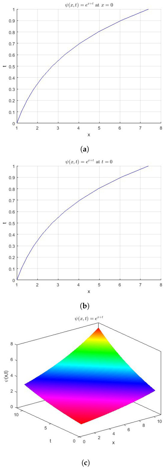
Figure 1. (a) The function $\psi (x,t)$; at $x=0$. (b) The function $\psi (x,t)$. at $t=0$. (c) The surface of the function $\psi (x,t)$.

• Partial integro-differential equation:

Assume that the partial integro-differential equation is denoted as follows,

$${\psi }_{xx}-{\psi }_{tt}+\psi +{\int }_0^x\psi \left(\zeta ,\eta \right)g\left(x-\zeta ,t-\eta \right)d\zeta d\eta =f\left(x,t\right),$$

(28)

B.C

$$\psi \left(0,t\right)=g_1\left(t\right),{\displaystyle \frac{\partial \psi \left(0,t\right)}{\partial x}}=g_2\left(t\right),$$

(29)

I.C

$$\psi \left(x,0\right)=f_1\left(x\right),{\displaystyle \frac{\partial \psi \left(x,0\right)}{\partial t}}=f_2\left(x\right),$$

(30)

where $g_1\left(t\right)$, $g_2\left(t\right), f_1\left(x\right)$, $f_2\left(x\right)$ and $f\left(x,t\right)$ are known functions. Employing the (NGLT) for Equation (28), (GLT) for Equation (29), and Natural Transform (NT) for Equation (30) and using Theorem 3, we yield

$$\begin{array}{ccc} & & {\displaystyle \frac{p^2}{u^2}}\Psi \left(p;u.s\right)-{\displaystyle \frac{p}{u^2}}\psi \left(0,s\right)-{\displaystyle \frac{1}{u}}{\psi }_x\left(0,s\right)\hfill \\ & & -{\displaystyle \frac{1}{s^2}}\Psi \left(p;u.s\right)+s^{\alpha -1}\psi \left(p;u,0\right)+s^{\alpha }{\psi }_t\left(p;u,0\right)\hfill \\ & & +\Psi \left(p;u.s\right)+{\displaystyle \frac{u}{s^{\alpha }}}G\left(p;u,s\right)\Psi \left(p;u,s\right)\hfill \\ & =& F\left(p;u,s\right),\hfill \end{array}$$

(31)

and

$$\psi \left(0,s\right)=G_1\left(s\right),{\displaystyle \frac{\partial \psi \left(0,s\right)}{\partial x}}=G_2\left(s\right),$$

(32)

$$\psi \left(p;u,0\right)=F_1\left(p;u\right),{\displaystyle \frac{\partial \psi \left(p;u,0\right)}{\partial t}}=F_2\left(p;u\right).$$

(33)

By replacing Equations (32) and (33) into Equation (31), we will gain

$$\begin{array}{ccc}\Psi \left(p;u.s\right)& =& {\displaystyle \frac{\left(\frac{p}{u^2}{G}_1\left(s\right)+\frac{1}{u}{G}_2\left(s\right)-s^{\alpha -1}{F}_1\left(p;u\right)\right)}{\left(\frac{p^2}{u^2}-\frac{1}{s^2}+1+\frac{u}{s^{\alpha }}G\left(p;u,s\right)\right)}}\hfill \\ & & -{\displaystyle \frac{\left(s^{\alpha }{F}_2\left(p;u\right)-F\left(p;u,s\right)\right)}{\left(\frac{p^2}{u^2}-\frac{1}{s^2}+1+\frac{u}{s^{\alpha }}G\left(p;u,s\right)\right)}},\hfill \end{array}$$

(34)

taking the inverse (NGLT) for Equation (34), we get

$$\begin{array}{ccc}\psi \left(x,t\right)& =& N_{p,u}^{-1}{G}_s^{-1}\left[{\displaystyle \frac{\left(\frac{p}{u^2}{G}_1\left(s\right)+\frac{1}{u}{G}_2\left(s\right)-s^{\alpha -1}{F}_1\left(p;u\right)\right)}{\left(\frac{p^2}{u^2}-\frac{1}{s^2}+1+\frac{u}{s^{\alpha }}G\left(p;u,s\right)\right)}}\right]\hfill \\ & & -N_{p,u}^{-1}{G}_s^{-1}\left[{\displaystyle \frac{\left(s^{\alpha }{F}_2\left(p;u\right)-F\left(p;u,s\right)\right)}{\left(\frac{p^2}{u^2}-\frac{1}{s^2}+1+\frac{u}{s^{\alpha }}G\left(p;u,s\right)\right)}}\right].\hfill \end{array}$$

(35)

This depends on if the (INLGT) for the right-hand side of Equation (35) exists. In the following example let $g\left(x-\zeta ,t-\eta \right)=e^{x-\zeta +t-\eta }$ and $f\left(x,t\right)=e^{x+t}+xt{e}^{x+t}$ as

Example 4.

Consider a partial integro-differential equation

$${\psi }_{xx}-{\psi }_{tt}+\psi +{\int }_0^x{\int }_0^t{e}^{x-\zeta +t-\eta }\psi \left(\zeta ,\eta \right)d\zeta d\eta =e^{x+t}+xt{e}^{x+t}$$

(36)

B.C

$$\psi \left(0,t\right)=e^t,{\displaystyle \frac{\partial \psi \left(0,t\right)}{\partial x}}=e^t,$$

(37)

I.C

$$\psi \left(x,0\right)=e^x,{\displaystyle \frac{\partial \psi \left(x,0\right)}{\partial t}}=e^x,$$

(38)

Employing the (NGLT) for Equation (36), (GLT) for Equation (37), (NT) for Equation (38), and using Theorem 3, we obtain,

$$\begin{array}{ccc} & & \left({\displaystyle \frac{p^2}{u^2}}-{\displaystyle \frac{1}{s^2}}+1+{\displaystyle \frac{us}{\left(p-u\right)\left(1-s\right)}}\right)\Psi \left(p;u.s\right)\hfill \\ & =& {\displaystyle \frac{s^{\alpha +1}}{\left(p-u\right)\left(1-s\right)}}\left({\displaystyle \frac{p^2}{u^2}}-{\displaystyle \frac{1}{s^2}}+1+{\displaystyle \frac{us}{\left(p-u\right)\left(1-s\right)}}\right),\hfill \end{array}$$

hence

$$\Psi \left(p;u.s\right)={\displaystyle \frac{s^{\alpha +1}}{\left(p-u\right)\left(1-s\right)}}$$

(39)

On using the inverse (NGLT) to Equation (39), we obtain

$$\psi \left(x,t\right)=e^{x+t}$$

Figure 2a depicts the variation solution of the partial integro-differential equation $\psi (x,t)$ in Equation (39) with time at $x=0$, whereas Figure 2b illustrates its variation with space at $t=0$. Figure 2c presents the three-dimensional surface plot of $\psi (x,t)$, providing a comprehensive representation of its behavior across both spatial and temporal domains.

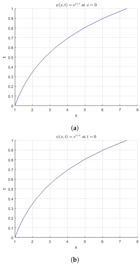
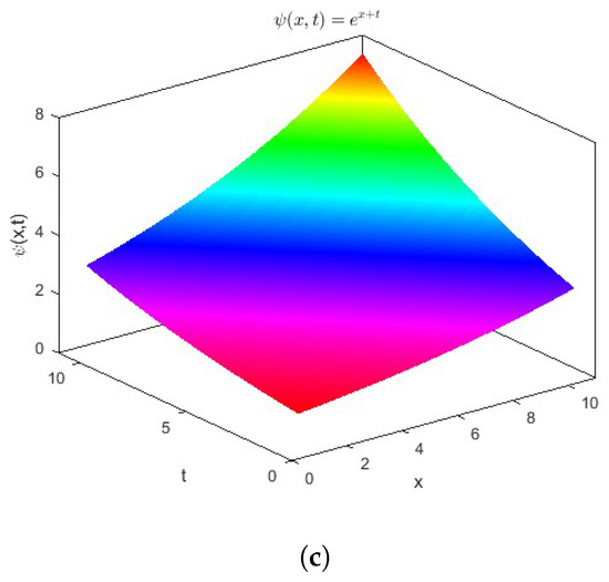
Figure 2. (a) The function $\psi (x,t)$. at $x=0$. (b) The function $\psi (x,t)$. at $t=0$. (c) The surface of the function $\psi (x,t)$.

4. The Natural Generalized-Laplace Transform Decomposition Method (NGLTDM) Applied to the Singular One-Dimensional Boussinesq Equation

In this section, we explain how to use the (NGLTDM) to solve a singular one-dimensional Boussinesq equation:

First problem: Let the following general linear singular one-dimensional Boussinesq equation be given by

$${\displaystyle \frac{{\partial }^2\psi }{\partial t^2}}-{\displaystyle \frac{1}{x}}{\displaystyle \frac{\partial }{\partial x}}\left(x{\displaystyle \frac{\partial \psi }{\partial x}}\right)+a\left(x\right){\displaystyle \frac{{\partial }^4\psi }{\partial x^4}}+b\left(x\right){\displaystyle \frac{{\partial }^4\psi }{\partial x^2\partial t^2}}=f\left(x,t\right),$$

(40)

with conditions

$$\psi \left(x,0\right)=f_1\left(x\right),{\displaystyle \frac{\partial \psi \left(x,0\right)}{\partial t}}=f_2\left(x\right),$$

(41)

where $f\left(x,t\right)$, $f_1\left(x\right), a\left(x\right)$, and $b\left(x\right)$ are given functions. To obtain the solution of Equation (40), the following steps are wanted.

Step 1. Multiply both sides of Equation (40) by $x,$ and using the (NGLT) with the new equation, (NT) for Equation (8), and using Equations (13) and (11), we get

$${\displaystyle \frac{d}{dp}}\left[{\displaystyle \frac{\Psi \left(p;u.s\right)}{s^2}}-s^{\alpha -1}{f}_1\left(p,u\right)-s^{\alpha }{f}_2\left(p,u\right)\right]=-{\displaystyle \frac{1}{u}}{\mathbf{N}}_x^{+}{G}_t\left[\Delta \right]+{\displaystyle \frac{d}{dp}}F\left(p;u,s\right),$$

(42)

where

$$\Delta ={\displaystyle \frac{\partial }{\partial x}}\left(x{\displaystyle \frac{\partial \psi }{\partial x}}\right)-xa\left(x\right){\displaystyle \frac{{\partial }^4\psi }{\partial x^4}}-xb\left(x\right){\displaystyle \frac{{\partial }^4\psi }{\partial x^2\partial t^2}},$$

by simplifying Equation (42), we have

$$\begin{array}{ccc}{\displaystyle \frac{d}{dp}}\left[{\displaystyle \frac{\Psi \left(p;u.s\right)}{s^2}}\right]& =& {\displaystyle \frac{d}{dp}}{s}^{\alpha -1}{f}_1\left(p,u\right)+{\displaystyle \frac{d}{dp}}{s}^{\alpha }{f}_2\left(p,u\right)\hfill \\ & & -{\displaystyle \frac{1}{u}}{\mathbf{N}}_x^{+}{G}_t\left[\Delta \right],\hfill \end{array}$$

(43)

by multiplying Equation (43) by $dp$ we have

$$\begin{array}{ccc}d\left[{\displaystyle \frac{\Psi \left(p;u.s\right)}{s^2}}\right]& =& d\left(s^{\alpha -1}{f}_1\left(p,u\right)\right)+d\left(s^{\alpha }{f}_2\left(p,u\right)\right)\hfill \\ & & -{\displaystyle \frac{1}{u}}{\mathbf{N}}_x^{+}{G}_t\left[\Delta \right]dp,\hfill \end{array}$$

(44)

by taking the integral for Equation (44) from 0 to p with regards toto p and multiplying the outcome by $s^2$, we get

$$\begin{array}{ccc}\Psi \left(p;u.s\right)& =& s^{\alpha +1}{f}_1\left(p,u\right)+s^{\alpha +2}{f}_2\left(p,u\right)-{\displaystyle \frac{s^2}{u}}{\int }_0^p{\mathbf{N}}_x^{+}{G}_t\left[\Delta \right]dp\hfill \\ & & +s^{2}F\left(p;u,s\right),\hfill \end{array}$$

(45)

where $F\left(p;u,s\right)$ is the (NGLT) of the function $f\left(x,t\right),$ and $F_1\left(p,u\right)$ and $F_2\left(p,u\right)$ are (NT) of the functions $f_1\left(x\right)$ and $f_2\left(x\right)$, respectively, and the (NGLT) with respect to $x$, t is defined by ${\mathbf{N}}_x^{+}{G}_t$.

Step 2. On using the inverse (NGLT) on both sides of Equation (45) we obtain

$$\psi \left(x,t\right)=f_1\left(x\right)+t{f}_2\left(x\right)+{\mathbf{N}}_{p,u}^{-1}{G}_s^{-1}\left[s^{2}F\left(p;u,s\right)\right]-{\mathbf{N}}_{p,u}^{-1}{G}_s^{-1}\left[{\displaystyle \frac{s^2}{u}}{\int }_0^p{\mathbf{N}}_x^{+}{G}_t\left[\Delta \right]dp\right].$$

(46)

where

$${\mathbf{N}}_{p,u}^{-1}{G}_s^{-1}\left[s^{\alpha +1}{f}_1\left(p,u\right)\right]=f_1\left(x\right),{\mathbf{N}}_{p,u}^{-1}{G}_s^{-1}\left[s^{\alpha +2}{f}_2\left(p,u\right)\right]=t{f}_2\left(x\right)$$

Step 3. The (NGLTDM) is defined as the solution $\psi (x,t)$ by the infinite series as follows:

$$\begin{array}{ccc}\psi \left(x,t\right)& =& {\displaystyle \sum }_{n=0}^{\infty }{\psi }_n\left(x,t\right).\hfill \\ & =& {\psi }_0\left(x,t\right)+{\psi }_1\left(x,t\right)+{\psi }_2\left(x,t\right)+\dots \hfill \end{array}$$

(47)

Replacing Equation (47) into Equation (46) and using

$$\Delta ={\displaystyle \frac{\partial }{\partial x}}\left(x{\displaystyle \frac{\partial \psi }{\partial x}}\right)-xa\left(x\right){\displaystyle \frac{{\partial }^4\psi }{\partial x^4}}-xb\left(x\right){\displaystyle \frac{{\partial }^4\psi }{\partial x^2\partial t^2}},$$

we have

$$\begin{array}{ccc}{\displaystyle \sum }_{n=0}^{\infty }{\psi }_n\left(x,t\right)& =& f_1\left(x\right)+t{f}_2\left(x\right)+{\mathbf{N}}_{p,u}^{-1}{G}_s^{-1}\left[s^{2}F\left(p;u,s\right)\right]\hfill \\ & & -{\mathbf{N}}_{p,u}^{-1}{G}_s^{-1}\left[{\displaystyle \frac{s^2}{u}}{\int }_0^p{\mathbf{N}}_x^{+}{G}_t\left[{\displaystyle \frac{\partial }{\partial x}}\left(x{\displaystyle \frac{\partial }{\partial x}}\left({\displaystyle \sum }_{n=0}^{\infty }{\psi }_n\left(x,t\right)\right)\right)\right]dp\right]\hfill \\ & & +{\mathbf{N}}_{p,u}^{-1}{G}_s^{-1}\left[{\displaystyle \frac{s^2}{u}}{\int }_0^p{\mathbf{N}}_x^{+}{G}_t\left[\left(xa\left(x\right){\displaystyle \frac{{\partial }^4}{\partial x^4}}\left({\displaystyle \sum }_{n=0}^{\infty }{\psi }_n\left(x,t\right)\right)\right)\right]dp\right]\hfill \\ & & +{\mathbf{N}}_{p,u}^{-1}{G}_s^{-1}\left[{\displaystyle \frac{s^2}{u}}{\int }_0^p{\mathbf{N}}_x^{+}{G}_t\left[\left(xb\left(x\right){\displaystyle \frac{{\partial }^4}{\partial x^2\partial t^2}}\left({\displaystyle \sum }_{n=0}^{\infty }{\psi }_n\left(x,t\right)\right)\right)\right]dp\right].\hfill \end{array}$$

(48)

Step 4. By comparing both sides of the Equation (48) we get

$${\psi }_0\left(x,t\right)=f_1\left(x\right)+t{f}_2\left(x\right)+{\mathbf{N}}_{p,u}^{-1}{G}_s^{-1}\left[{\displaystyle \frac{u^2}{p^2}}F\left(p;u,s\right)\right]$$

(49)

at $n=0$

$$\begin{array}{ccc}{\psi }_1& =& -{\mathbf{N}}_{p,u}^{-1}{G}_s^{-1}\left[{\displaystyle \frac{s^2}{u}}{\int }_0^p{\mathbf{N}}_x^{+}{G}_t\left[{\displaystyle \frac{\partial }{\partial x}}\left(x{\displaystyle \frac{\partial }{\partial x}}\left({\psi }_0\left(x,t\right)\right)\right)\right]dp\right]\hfill \\ & & +{\mathbf{N}}_{p,u}^{-1}{G}_s^{-1}\left[{\displaystyle \frac{s^2}{u}}{\int }_0^p{\mathbf{N}}_x^{+}{G}_t\left[\left(xa\left(x\right){\displaystyle \frac{{\partial }^4}{\partial x^4}}\left({\psi }_0\left(x,t\right)\right)\right)\right]dp\right]\hfill \\ & & +{\mathbf{N}}_{p,u}^{-1}{G}_s^{-1}\left[{\displaystyle \frac{s^2}{u}}{\int }_0^p{\mathbf{N}}_x^{+}{G}_t\left[\left(xb\left(x\right){\displaystyle \frac{{\partial }^4}{\partial x^2\partial t^2}}\left({\psi }_0\left(x,t\right)\right)\right)\right]dp\right],\hfill \end{array}$$

(50)

at $n=1$

$$\begin{array}{ccc}{\psi }_2& =& -{\mathbf{N}}_{p,u}^{-1}{G}_s^{-1}\left[{\displaystyle \frac{s^2}{u}}{\int }_0^p{\mathbf{N}}_x^{+}{G}_t\left[{\displaystyle \frac{\partial }{\partial x}}\left(x{\displaystyle \frac{\partial }{\partial x}}\left({\psi }_1\left(x,t\right)\right)\right)\right]dp\right]\hfill \\ & & +{\mathbf{N}}_{p,u}^{-1}{G}_s^{-1}\left[{\displaystyle \frac{s^2}{u}}{\int }_0^p{\mathbf{N}}_x^{+}{G}_t\left[\left(xa\left(x\right){\displaystyle \frac{{\partial }^4}{\partial x^4}}\left({\psi }_1\left(x,t\right)\right)\right)\right]dp\right]\hfill \\ & & +{\mathbf{N}}_{p,u}^{-1}{G}_s^{-1}\left[{\displaystyle \frac{s^2}{u}}{\int }_0^p{\mathbf{N}}_x^{+}{G}_t\left[\left(xb\left(x\right){\displaystyle \frac{{\partial }^4}{\partial x^2\partial t^2}}\left({\psi }_1\left(x,t\right)\right)\right)\right]dp\right],\hfill \end{array}$$

(51)

at $n=2$

$$\begin{array}{ccc}{\psi }_3& =& -{\mathbf{N}}_{p,u}^{-1}{G}_s^{-1}\left[{\displaystyle \frac{s^2}{u}}{\int }_0^p{\mathbf{N}}_x^{+}{G}_t\left[{\displaystyle \frac{\partial }{\partial x}}\left(x{\displaystyle \frac{\partial }{\partial x}}\left({\psi }_2\left(x,t\right)\right)\right)\right]dp\right]\hfill \\ & & +{\mathbf{N}}_{p,u}^{-1}{G}_s^{-1}\left[{\displaystyle \frac{s^2}{u}}{\int }_0^p{\mathbf{N}}_x^{+}{G}_t\left[\left(xa\left(x\right){\displaystyle \frac{{\partial }^4}{\partial x^4}}\left({\psi }_2\left(x,t\right)\right)\right)\right]dp\right]\hfill \\ & & +{\mathbf{N}}_{p,u}^{-1}{G}_s^{-1}\left[{\displaystyle \frac{s^2}{u}}{\int }_0^p{\mathbf{N}}_x^{+}{G}_t\left[\left(xb\left(x\right){\displaystyle \frac{{\partial }^4}{\partial x^2\partial t^2}}\left({\psi }_2\left(x,t\right)\right)\right)\right]dp\right],\hfill \end{array}$$

(52)

$$\begin{array}{ccc} & & ·\hfill \\ & & ·\hfill \\ & & ·\hfill \end{array}$$

at $n=n-1$

$$\begin{array}{ccc}{\psi }_n& =& -{\mathbf{N}}_{p,u}^{-1}{G}_s^{-1}\left[{\displaystyle \frac{s^2}{u}}{\int }_0^p{\mathbf{N}}_x^{+}{G}_t\left[{\displaystyle \frac{\partial }{\partial x}}\left(x{\displaystyle \frac{\partial }{\partial x}}\left({\psi }_{n-1}\left(x,t\right)\right)\right)\right]dp\right]\hfill \\ & & +{\mathbf{N}}_{p,u}^{-1}{G}_s^{-1}\left[{\displaystyle \frac{s^2}{u}}{\int }_0^p{\mathbf{N}}_x^{+}{G}_t\left[\left(xa\left(x\right){\displaystyle \frac{{\partial }^4}{\partial x^4}}\left({\psi }_{n-1}\left(x,t\right)\right)\right)\right]dp\right]\hfill \\ & & +{\mathbf{N}}_{p,u}^{-1}{G}_s^{-1}\left[{\displaystyle \frac{s^2}{u}}{\int }_0^p{\mathbf{N}}_x^{+}{G}_t\left[\left(xb\left(x\right){\displaystyle \frac{{\partial }^4}{\partial x^2\partial t^2}}\left({\psi }_{n-1}\left(x,t\right)\right)\right)\right]dp\right],\hfill \end{array}$$

(53)

Consequently, the approximate solution to Equation (3) is obtained by substituting Equations (49)–(53) into Equation (47) as outlined below

$$\psi ={\psi }_0+{\psi }_1+{\psi }_2+\dots +{\psi }_n={\displaystyle \sum }_{n=0}^{\infty }{\psi }_n\left(x,t\right),$$

(54)

where the (INGLT) is denoted by ${\mathbf{N}}_{p;u}^{-1}{G}_s^{-1}$. Here, we provided that the (INGLT) exists for each term on the right-hand side of all the above equations. We solve the following example to demonstrate the applicability of this method to solving the singular one-dimensional Boussinesq equation.

Convergence:

Theorem 5.

Let $\psi \left(x,t\right)\in B$ and $\alpha \in \left(0,1\right),$ in which B indicates the Banach space and suppose that $\psi \left(x,t\right)$ is the exact solution to Equation (55). The obtained findings ${\displaystyle {\displaystyle \sum }_{n=0}^{\infty }}{\psi }_n\left(x,t\right)$ are converged to $\psi \left(x,t\right)$ if ${\psi }_n\left(x,t\right)\le {\psi }_{n-1}\left(x,t\right)$, $\forall n\in \mathbb{N},$ the Cauchy sequence $S_n\in B$, so that, $∥{\psi }_n\left(x,t\right)∥\le \alpha ∥{\psi }_{n-1}\left(x,t\right)∥$, $\forall n\in \mathbb{N}.$

Proof. 

Indicate that $S_n$ is a Cauchy sequence in $B,$ using the definition of the sequence

$S_n={\displaystyle {\displaystyle \sum }_{n=0}^{\infty }}{\psi }_n\left(x,t\right)$ of partial sums of the series of Equation (54) as follows

$$\begin{array}{ccc}{S}_0& =& {\psi }_0\left(x,t\right)\hfill \\ S_1& =& {\psi }_0\left(x,t\right)+{\psi }_1\left(x,t\right)\hfill \\ S_2& =& {\psi }_0\left(x,t\right)+{\psi }_1\left(x,t\right)+{\psi }_2\left(x,t\right)\hfill \\ & & \begin{array}{c}.\\ .\\ .\end{array}\hfill \\ S_n& =& {\psi }_0+{\psi }_1+{\psi }_2+\dots +{\psi }_n,\hfill \end{array}$$

to illustrate that ${\left\{S_n\right\}}_{n=0}^{\infty }$ is a Cauchy sequence in Banach space B. Therefore, we consider

$$\begin{array}{ccc}∥S_{n+1}-S_n∥& =& ∥{\psi }_n\left(x,t\right)∥\le \alpha ∥{\psi }_{n-1}\left(x,t\right)∥\hfill \\ & \le & {\alpha }^2∥{\psi }_{n-2}\left(x,t\right)∥\le \dots \hfill \\ & \le & {\alpha }^{n+1}∥{\psi }_0\left(x,t\right)∥,\hfill \end{array}$$

for a partial sum $S_n,$ and $S_m$ by using the above triangle inequality for $n\ge m,$ we obtain

$$\begin{array}{ccc}∥S_n-S_m∥& =& ∥S_n-S_{n-1}+S_{n-1}-S_{n-2}+\dots +S_{m+2}-S_{m+1}+S_{m+1}-S_m∥,\hfill \\ & \le & ∥S_n-S_{n-1}∥+∥S_{n-1}-S_{n-2}∥+\hfill \\ & & +\dots +∥S_{m+2}-S_{m+1}∥+∥S_{m+1}-S_m∥,\hfill \\ & \le & {\alpha }^n∥{\psi }_0∥+{\alpha }^{n-1}∥{\psi }_0∥+\dots +{\alpha }^{m+1}∥{\psi }_0∥+{\alpha }^m∥{\psi }_0∥,\hfill \\ & \le & \left({\alpha }^n+{\alpha }^{n-1}+\dots +{\alpha }^{m+1}+{\alpha }^m\right)∥{\psi }_0∥\hfill \\ & =& {\alpha }^m\left({\alpha }^{n-m}+{\alpha }^{n-m-1}+\alpha \dots +1\right)∥{\psi }_0∥,\hfill \\ & \le & {\alpha }^m\left({\displaystyle \frac{1-{\alpha }^{n-m}}{1-\alpha }}\right)∥{\psi }_0∥,\hfill \end{array}$$

from $0\le \alpha <1$ we realize that $1-{\alpha }^{n-m}<1,$ thus

$$∥S_n-S_m∥\le {\displaystyle \frac{{\alpha }^m}{1-\alpha }}∥{\psi }_0∥,$$

since ${\psi }_0$ bounded, consequently $∥S_n-S_m∥\to 0$ at $n,m\to \infty$. Hence, the sequence $\left\{S_m\right\}$ represents a Cauchy sequence in the Banach space B; then the series solution of Equation (54) is converged, which completes the proof of theorem.  □

In the next example, we apply our method.

Example 5.

Consider a singular one-dimensional Boussinesq equation

$${\psi }_{tt}-{\displaystyle \frac{1}{x}}{\left(x{\psi }_x\right)}_x+{\psi }_{xxxx}-{\psi }_{xxtt}=-x^2\sin t-2\sin t,$$

(55)

subject to initial condition

$$\psi \left(x,0\right)=0,{\psi }_t\left(x,0\right)=x^2.$$

(56)

by multiplying Equation (55) by x and using the (NGLT) to the new equation, (NT) for Equation (56), and using the utilizing Equations (13) and (11), we obtain,

$$\begin{array}{ccc}{\mathbf{N}}_x^{+}{G}_t\left[x{\psi }_{tt}\right]& =& {\mathbf{N}}_x^{+}{G}_t\left[{\left(x{\psi }_x\right)}_x-x{\psi }_{xxxx}+x{\psi }_{xxtt}\right]\hfill \\ & & -{\mathbf{N}}_x^{+}{G}_t\left(x^3\left(t-{\displaystyle \frac{t^3}{3!}}+{\displaystyle \frac{t^5}{5!}}-\cdots \right)\right)\hfill \\ & & -2{\mathbf{N}}_x^{+}{G}_t\left(x\left(t-{\displaystyle \frac{t^3}{3!}}+{\displaystyle \frac{t^5}{5!}}-\cdots \right)\right),\hfill \end{array}$$

(57)

hence

$$\begin{array}{ccc}{\displaystyle \frac{d}{dp}}\left[{\displaystyle \frac{\Psi \left(p;u.s\right)}{s^2}}-{\displaystyle \frac{2u^2{s}^{\alpha }}{p^3}}\right]& =& -{\displaystyle \frac{1}{u}}{\mathbf{N}}_x^{+}{G}_t\left[{\left(x{\psi }_x\right)}_x-x{\psi }_{xxxx}+x{\psi }_{xxtt}\right]\hfill \\ & & +{\displaystyle \frac{3!u^2}{p^4}}\left(s^{\alpha +2}-s^{\alpha +4}+s^{\alpha +6}-\cdots \right)\hfill \\ & & +{\displaystyle \frac{2}{p^2}}\left(s^{\alpha +2}-s^{\alpha +4}+s^{\alpha +6}-\cdots \right).\hfill \end{array}$$

(58)

by integrating both sides of Equation (58) from 0 to p with respect to p, we have

$$\begin{array}{ccc}\Psi \left(p;u.s\right)& =& {\displaystyle \frac{2u^2{s}^{\alpha +2}}{p^3}}-{\displaystyle \frac{s^2}{u}}{\int }_0^p{\mathbf{N}}_x^{+}{G}_t\left[{\left(x{\psi }_x\right)}_x-x{\psi }_{xxxx}+x{\psi }_{xxtt}\right]dp\hfill \\ & & -{\displaystyle \frac{2!u^2}{p^3}}\left(s^{\alpha +4}-s^{\alpha +6}+s^{\alpha +8}-\cdots \right)\hfill \\ & & -{\displaystyle \frac{2}{p}}\left(s^{\alpha +4}-s^{\alpha +6}+s^{\alpha +8}-\cdots \right).\hfill \end{array}$$

(59)

On using the (INGLT) to Equation (59), we gain

$$\begin{array}{ccc}\psi \left(x,t\right)& =& -{\mathbf{N}}_{p;u}^{-1}{G}_s^{-1}\left[{\displaystyle \frac{s^2}{u}}{\int }_0^p{\mathbf{N}}_x^{+}{G}_t\left[{\left(x{\psi }_x\right)}_x-x{\psi }_{xxxx}+x{\psi }_{xxtt}\right]dp\right]\hfill \\ & & +x^{2}t-x^2\left({\displaystyle \frac{t^3}{3!}}-{\displaystyle \frac{t^5}{5!}}+{\displaystyle \frac{t^7}{7!}}-\cdots \right)\hfill \\ & & -2\left({\displaystyle \frac{t^3}{3!}}-{\displaystyle \frac{t^5}{5!}}+{\displaystyle \frac{t^7}{7!}}-\cdots \right),\hfill \end{array}$$

(60)

putting Equation (47) into Equation (60) we will get

$$\begin{array}{ccc}{\displaystyle \sum }_{n=0}^{\infty }{\psi }_n\left(x,t\right)& =& -{\mathbf{N}}_{p;u}^{-1}{G}_s^{-1}\left[{\displaystyle \frac{s^2}{u}}{\int }_0^p{\mathbf{N}}_x^{+}{G}_t\left[{\displaystyle \frac{\partial }{\partial x}}\left(x{\displaystyle \frac{\partial }{\partial x}}{\displaystyle \sum }_{n=0}^{\infty }{\psi }_n\left(x,t\right)\right)\right]dp\right]\hfill \\ & & +{\mathbf{N}}_{p;u}^{-1}{G}_s^{-1}\left[{\displaystyle \frac{s^2}{u}}{\int }_0^p{\mathbf{N}}_x^{+}{G}_t\left[x{\displaystyle \frac{{\partial }^4}{\partial x^4}}\left({\displaystyle \sum }_{n=0}^{\infty }{\psi }_n\left(x,t\right)\right)\right]dp\right]\hfill \\ & & -{\mathbf{N}}_{p;u}^{-1}{G}_s^{-1}\left[{\displaystyle \frac{s^2}{u}}{\int }_0^p{\mathbf{N}}_x^{+}{G}_t\left[x{\displaystyle \frac{{\partial }^4}{\partial x^2\partial t^2}}\left({\displaystyle \sum }_{n=0}^{\infty }{\psi }_n\left(x,t\right)\right)\right]dp\right]\hfill \\ & & +x^{2}t-x^2\left({\displaystyle \frac{t^3}{3!}}-{\displaystyle \frac{t^5}{5!}}+{\displaystyle \frac{t^7}{7!}}-\cdots \right)-2\left({\displaystyle \frac{t^3}{3!}}-{\displaystyle \frac{t^5}{5!}}+{\displaystyle \frac{t^7}{7!}}-\cdots \right)\hfill \end{array}$$

(61)

By using the (NGLTDM), we have

$${\psi }_0=x^{2}t-x^2\left({\displaystyle \frac{t^3}{3!}}-{\displaystyle \frac{t^5}{5!}}+{\displaystyle \frac{t^7}{7!}}-\cdots \right)-2\left({\displaystyle \frac{t^3}{3!}}-{\displaystyle \frac{t^5}{5!}}+{\displaystyle \frac{t^7}{7!}}-\cdots \right),$$

and

$$\begin{array}{ccc}{\psi }_{n+1}& =& -{\mathbf{N}}_{p;u}^{-1}{G}_s^{-1}\left[{\displaystyle \frac{s^2}{u}}{\int }_0^p{\mathbf{N}}_x^{+}{G}_t\left[{\displaystyle \frac{\partial }{\partial x}}\left(x{\displaystyle \frac{\partial }{\partial x}}{\displaystyle \sum }_{n=0}^{\infty }{\psi }_n\left(x,t\right)\right)\right]dp\right]\hfill \\ & & +{\mathbf{N}}_{p;u}^{-1}{G}_s^{-1}\left[{\displaystyle \frac{s^2}{u}}{\int }_0^p{\mathbf{N}}_x^{+}{G}_t\left[x{\displaystyle \frac{{\partial }^4}{\partial x^4}}\left({\displaystyle \sum }_{n=0}^{\infty }{\psi }_n\left(x,t\right)\right)\right]dp\right]\hfill \\ & & -{\mathbf{N}}_{p;u}^{-1}{G}_s^{-1}\left[{\displaystyle \frac{s^2}{u}}{\int }_0^p{\mathbf{N}}_x^{+}{G}_t\left[x{\displaystyle \frac{{\partial }^4}{\partial x^2\partial t^2}}\left({\displaystyle \sum }_{n=0}^{\infty }{\psi }_n\left(x,t\right)\right)\right]dp\right],\hfill \end{array}$$

now the components of the series solution at $n=0,$ we have

$$\begin{array}{ccc}{\psi }_1& =& -{\mathbf{N}}_{p;u}^{-1}{G}_s^{-1}\left[{\displaystyle \frac{s^2}{u}}{\int }_0^p{\mathbf{N}}_x^{+}{G}_t\left[{\displaystyle \frac{\partial }{\partial x}}\left(x{\displaystyle \frac{\partial }{\partial x}}{\psi }_0\right)\right]dp\right]\hfill \\ & & +{\mathbf{N}}_{p;u}^{-1}{G}_s^{-1}\left[{\displaystyle \frac{s^2}{u}}{\int }_0^p{\mathbf{N}}_x^{+}{G}_t\left[x{\displaystyle \frac{{\partial }^4}{\partial x^4}}\left({\psi }_0\right)\right]dp\right]\hfill \\ & & -{\mathbf{N}}_{p;u}^{-1}{G}_s^{-1}\left[{\displaystyle \frac{s^2}{u}}{\int }_0^p{\mathbf{N}}_x^{+}{G}_t\left[x{\displaystyle \frac{{\partial }^4}{\partial x^2\partial t^2}}\left({\psi }_0\right)\right]dp\right]\hfill \\ & =& -{\mathbf{N}}_{p;u}^{-1}{G}_s^{-1}\left[{\displaystyle \frac{s^2}{u}}{\int }_0^p{\mathbf{N}}_x^{+}{G}_t\left[2x\left(t-{\displaystyle \frac{t^3}{3!}}+{\displaystyle \frac{t^5}{5!}}-\cdots \right)\right]dp\right]\hfill \\ & =& {\mathbf{N}}_{p;u}^{-1}{G}_s^{-1}\left[{\displaystyle \frac{2}{p}}\left(s^{\alpha +4}-s^{\alpha +6}+s^{\alpha +8}-\cdots \right)\right]\hfill \\ & =& 2\left({\displaystyle \frac{t^3}{3!}}-{\displaystyle \frac{t^5}{5!}}+{\displaystyle \frac{t^7}{7!}}-\cdots \right)\hfill \end{array}$$

by similar way, at $n=1,$ we get

$$\begin{array}{ccc}{\psi }_2& =& -{\mathbf{N}}_{p;u}^{-1}{G}_s^{-1}\left[{\displaystyle \frac{s^2}{u}}{\int }_0^p{\mathbf{N}}_x^{+}{G}_t\left[{\displaystyle \frac{\partial }{\partial x}}\left(x{\displaystyle \frac{\partial }{\partial x}}{\psi }_1\right)\right]dp\right]\hfill \\ & & +{\mathbf{N}}_{p;u}^{-1}{G}_s^{-1}\left[{\displaystyle \frac{s^2}{u}}{\int }_0^p{\mathbf{N}}_x^{+}{G}_t\left[x{\displaystyle \frac{{\partial }^4}{\partial x^4}}\left({\psi }_1\right)\right]dp\right]\hfill \\ & & -{\mathbf{N}}_{p;u}^{-1}{G}_s^{-1}\left[{\displaystyle \frac{s^2}{u}}{\int }_0^p{\mathbf{N}}_x^{+}{G}_t\left[x{\displaystyle \frac{{\partial }^4}{\partial x^2\partial t^2}}\left({\psi }_1\right)\right]dp\right]\hfill \\ {\psi }_2& =& \mathbf{0},\hfill \end{array}$$

and at $n=2,$

$${\psi }_3={\mathbf{N}}_{p;u}^{-1}{G}_s^{-1}\left[{\displaystyle \frac{s^2}{u}}{\int }_0^p{\mathbf{N}}_x^{+}{G}_t\left[0\right]dp\right]=0.$$

Therefore, the approximate solution of Equation (55) granted by

$$\begin{array}{ccc}{\displaystyle \sum }_{n=0}^{\infty }{\psi }_n\left(x,t\right)& =& {\psi }_0+{\psi }_1+{\psi }_2+\cdots \hfill \\ & =& x^{2}t-x^2\left({\displaystyle \frac{t^3}{3!}}-{\displaystyle \frac{t^5}{5!}}+{\displaystyle \frac{t^7}{7!}}-\cdots \right)\hfill \end{array}$$

Hence, the exact solution is given by

$$\begin{array}{ccc}\psi \left(x,t\right)& =& x^2\left(t-{\displaystyle \frac{t^3}{3!}}-{\displaystyle \frac{t^5}{5!}}+{\displaystyle \frac{t^7}{7!}}-\cdots \right),\hfill \\ & =& x^2\sin t.\hfill \end{array}$$

Figure 3a illustrates the variation of the function $\psi (x,t)$, as defined in Equation (55), with time at $x=0$, while Figure 2c displays the three-dimensional surface plot of $\psi (x,t)$, offering a comprehensive depiction of its behavior across both space and time domains.

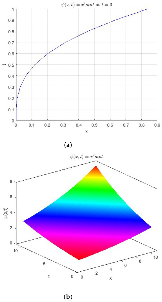
Figure 3. (a) The function $\psi (x,t)$. at $x=0$. (b) The surface of the function $\psi (x,t)$.

Below, we will solve Example 5, using Equation (16) and the (NGLTDM). By the multiplication of Equation (55) by x, the (NGLT) to the new equation, and (NT) for Equations (11), (16) and (56), one can obtain,

$$\begin{array}{ccc}{\displaystyle \frac{u}{p{s}^2}}{\displaystyle \frac{d}{du}}\left(u\Psi \left(p;u,s\right)\right)& =& {\displaystyle \frac{u{s}^{\alpha -1}}{p}}{\displaystyle \frac{d}{du}}\left(u\psi \left(p;u,0\right)\right)+{\displaystyle \frac{u{s}^{\alpha }}{p}}{\displaystyle \frac{d}{du}}\left(u{\psi }_t\left(p;u,0\right)\right)\hfill \\ & & +{\mathbf{N}}_x^{+}{G}_t\left[{\left(x{\psi }_x\right)}_x-x{\psi }_{xxxx}+x{\psi }_{xxtt}\right]\hfill \\ & & -{\mathbf{N}}_x^{+}{G}_t\left(x^3\left(t-{\displaystyle \frac{t^3}{3!}}+{\displaystyle \frac{t^5}{5!}}-\cdots \right)\right)\hfill \\ & & -2{\mathbf{N}}_x^{+}{G}_t\left(x\left(t-{\displaystyle \frac{t^3}{3!}}+{\displaystyle \frac{t^5}{5!}}-\cdots \right)\right),\hfill \end{array}$$

hence

$$\begin{array}{ccc}{\displaystyle \frac{d}{du}}\left(u\Psi \left(p;u,s\right)\right)={\displaystyle \frac{6u^2{s}^{\alpha +2}}{p^3}}& & +{\displaystyle \frac{p{s}^2}{u}}{\mathbf{N}}_x^{+}{G}_t\left[{\left(x{\psi }_x\right)}_x-x{\psi }_{xxxx}+x{\psi }_{xxtt}\right]\hfill \\ & & -{\displaystyle \frac{3!u^2}{p^3}}\left(s^{\alpha +4}-s^{\alpha +6}+s^{\alpha +8}-\cdots \right)\hfill \\ & & -{\displaystyle \frac{2}{p}}\left(s^{\alpha +4}-s^{\alpha +6}+s^{\alpha +8}-\cdots \right),\hfill \end{array}$$

(62)

by integrating both sides of Equation (62) from 0 to u with respect to u, divide the result by $u,$ and using the (INGLT) we will get

$$\begin{array}{ccc}\psi \left(x,t\right)& =& x^{2}t-{\mathbf{N}}_{p;u}^{-1}{G}_s^{-1}\left[{\displaystyle \frac{1}{u}}{\int }_0^u{\displaystyle \frac{p{s}^2}{u}}{\mathbf{N}}_x^{+}{G}_t\left[{\left(x{\psi }_x\right)}_x-x{\psi }_{xxxx}+x{\psi }_{xxtt}\right]du\right]\hfill \\ & & -x^2\left({\displaystyle \frac{t^3}{3!}}-{\displaystyle \frac{t^5}{5!}}+{\displaystyle \frac{t^7}{7!}}-\cdots \right)\hfill \\ & & -2\left({\displaystyle \frac{t^3}{3!}}-{\displaystyle \frac{t^5}{5!}}+{\displaystyle \frac{t^7}{7!}}-\cdots \right),\hfill \end{array}$$

(63)

by substituting Equation (47) into Equation (63) one can get

$$\begin{array}{ccc}{\displaystyle \sum }_{n=0}^{\infty }{\psi }_n\left(x,t\right)& =& {\mathbf{N}}_{p;u}^{-1}{G}_s^{-1}\left[{\displaystyle \frac{1}{u}}{\int }_0^u{\displaystyle \frac{p{s}^2}{u}}{\mathbf{N}}_x^{+}{G}_t\left[{\displaystyle \frac{\partial }{\partial x}}\left(x{\displaystyle \frac{\partial }{\partial x}}{\displaystyle \sum }_{n=0}^{\infty }{\psi }_n\left(x,t\right)\right)\right]du\right]\hfill \\ & & +{\mathbf{N}}_{p;u}^{-1}{G}_s^{-1}\left[{\displaystyle \frac{1}{u}}{\int }_0^u{\displaystyle \frac{p{s}^2}{u}}{\mathbf{N}}_x^{+}{G}_t\left[x{\displaystyle \frac{{\partial }^4}{\partial x^4}}\left({\displaystyle \sum }_{n=0}^{\infty }{\psi }_n\left(x,t\right)\right)\right]du\right]\hfill \\ & & -{\mathbf{N}}_{p;u}^{-1}{G}_s^{-1}\left[{\displaystyle \frac{1}{u}}{\int }_0^u{\displaystyle \frac{p{s}^2}{u}}{\mathbf{N}}_x^{+}{G}_t\left[x{\displaystyle \frac{{\partial }^4}{\partial x^2\partial t^2}}\left({\displaystyle \sum }_{n=0}^{\infty }{\psi }_n\left(x,t\right)\right)\right]du\right]\hfill \\ & & +x^{2}t-x^2\left({\displaystyle \frac{t^3}{3!}}-{\displaystyle \frac{t^5}{5!}}+{\displaystyle \frac{t^7}{7!}}-\cdots \right)-2\left({\displaystyle \frac{t^3}{3!}}-{\displaystyle \frac{t^5}{5!}}+{\displaystyle \frac{t^7}{7!}}-\cdots \right).\hfill \end{array}$$

(64)

By utilizing the (NGLTDM), we have

$${\psi }_0=x^{2}t-x^2\left({\displaystyle \frac{t^3}{3!}}-{\displaystyle \frac{t^5}{5!}}+{\displaystyle \frac{t^7}{7!}}-\cdots \right)-2\left({\displaystyle \frac{t^3}{3!}}-{\displaystyle \frac{t^5}{5!}}+{\displaystyle \frac{t^7}{7!}}-\cdots \right),$$

and

$$\begin{array}{ccc}{\psi }_{n+1}& =& {\mathbf{N}}_{p;u}^{-1}{G}_s^{-1}\left[{\displaystyle \frac{1}{u}}{\int }_0^u{\displaystyle \frac{p{s}^2}{u}}{\mathbf{N}}_x^{+}{G}_t\left[{\displaystyle \frac{\partial }{\partial x}}\left(x{\displaystyle \frac{\partial }{\partial x}}{\displaystyle \sum }_{n=0}^{\infty }{\psi }_n\left(x,t\right)\right)\right]du\right]\hfill \\ & & +{\mathbf{N}}_{p;u}^{-1}{G}_s^{-1}\left[{\displaystyle \frac{1}{u}}{\int }_0^u{\displaystyle \frac{p{s}^2}{u}}{\mathbf{N}}_x^{+}{G}_t\left[x{\displaystyle \frac{{\partial }^4}{\partial x^4}}\left({\displaystyle \sum }_{n=0}^{\infty }{\psi }_n\left(x,t\right)\right)\right]du\right]\hfill \\ & & -{\mathbf{N}}_{p;u}^{-1}{G}_s^{-1}\left[{\displaystyle \frac{1}{u}}{\int }_0^u{\displaystyle \frac{p{s}^2}{u}}{\mathbf{N}}_x^{+}{G}_t\left[x{\displaystyle \frac{{\partial }^4}{\partial x^2\partial t^2}}\left({\displaystyle \sum }_{n=0}^{\infty }{\psi }_n\left(x,t\right)\right)\right]du\right],\hfill \end{array}$$

by using the components of the series solution at $n=0,$ we will get

$$\begin{array}{ccc}{\psi }_1& =& {\mathbf{N}}_{p;u}^{-1}{G}_s^{-1}\left[{\displaystyle \frac{1}{u}}{\int }_0^u{\displaystyle \frac{p{s}^2}{u}}{\mathbf{N}}_x^{+}{G}_t\left[{\displaystyle \frac{\partial }{\partial x}}\left(x{\displaystyle \frac{\partial }{\partial x}}{\psi }_0\right)\right]du\right]\hfill \\ & & +{\mathbf{N}}_{p;u}^{-1}{G}_s^{-1}\left[{\displaystyle \frac{1}{u}}{\int }_0^u{\displaystyle \frac{p{s}^2}{u}}{\mathbf{N}}_x^{+}{G}_t\left[x{\displaystyle \frac{{\partial }^4}{\partial x^4}}\left({\psi }_0\right)\right]du\right]\hfill \\ & & -{\mathbf{N}}_{p;u}^{-1}{G}_s^{-1}\left[{\displaystyle \frac{1}{u}}{\int }_0^u{\displaystyle \frac{p{s}^2}{u}}{\mathbf{N}}_x^{+}{G}_t\left[x{\displaystyle \frac{{\partial }^4}{\partial x^2\partial t^2}}\left({\psi }_0\right)\right]du\right]\hfill \\ & =& -{\mathbf{N}}_{p;u}^{-1}{G}_s^{-1}\left[{\displaystyle \frac{1}{u}}{\int }_0^u{\displaystyle \frac{p{s}^2}{u}}{\mathbf{N}}_x^{+}{G}_t\left[2x\left(t-{\displaystyle \frac{t^3}{3!}}+{\displaystyle \frac{t^5}{5!}}-\cdots \right)\right]du\right]\hfill \\ & =& {\mathbf{N}}_{p;u}^{-1}{G}_s^{-1}\left[{\displaystyle \frac{2}{p}}\left(s^{\alpha +4}-s^{\alpha +6}+s^{\alpha +8}-\cdots \right)\right]\hfill \\ & =& 2\left({\displaystyle \frac{t^3}{3!}}-{\displaystyle \frac{t^5}{5!}}+{\displaystyle \frac{t^7}{7!}}-\cdots \right),\hfill \end{array}$$

in a similar way, at $n=1,$ we get

$$\begin{array}{ccc}{\psi }_2& =& {\mathbf{N}}_{p;u}^{-1}{G}_s^{-1}\left[{\displaystyle \frac{1}{u}}{\int }_0^u{\displaystyle \frac{p{s}^2}{u}}{\mathbf{N}}_x^{+}{G}_t\left[{\displaystyle \frac{\partial }{\partial x}}\left(x{\displaystyle \frac{\partial }{\partial x}}{\psi }_1\right)\right]du\right]\hfill \\ & & +{\mathbf{N}}_{p;u}^{-1}{G}_s^{-1}\left[{\displaystyle \frac{1}{u}}{\int }_0^u{\displaystyle \frac{p{s}^2}{u}}{\mathbf{N}}_x^{+}{G}_t\left[x{\displaystyle \frac{{\partial }^4}{\partial x^4}}\left({\psi }_1\right)\right]du\right]\hfill \\ & & -{\mathbf{N}}_{p;u}^{-1}{G}_s^{-1}\left[{\displaystyle \frac{1}{u}}{\int }_0^u{\displaystyle \frac{p{s}^2}{u}}{\mathbf{N}}_x^{+}{G}_t\left[x{\displaystyle \frac{{\partial }^4}{\partial x^2\partial t^2}}\left({\psi }_1\right)\right]du\right]\hfill \\ {\psi }_2& =& 0,\hfill \end{array}$$

and at $n=2,$

$${\psi }_3={\mathbf{N}}_{p;u}^{-1}{G}_s^{-1}\left[{\displaystyle \frac{s^2}{u}}{\int }_0^p{\mathbf{N}}_x^{+}{G}_t\left[0\right]dp\right]=0.$$

In a similar way, we find that ${\psi }_4=0,$${\psi }_5=0.$ Consequently the approximate solution of Equation (55) is granted by

$$\begin{array}{ccc}{\displaystyle \sum }_{n=0}^{\infty }{\psi }_n\left(x,t\right)& =& {\psi }_0+{\psi }_1+{\psi }_2+\cdots \hfill \\ & =& x^{2}t-x^2\left({\displaystyle \frac{t^3}{3!}}-{\displaystyle \frac{t^5}{5!}}+{\displaystyle \frac{t^7}{7!}}-\cdots \right)-2\left({\displaystyle \frac{t^3}{3!}}-{\displaystyle \frac{t^5}{5!}}+{\displaystyle \frac{t^7}{7!}}-\cdots \right)\hfill \\ & & +2\left({\displaystyle \frac{t^3}{3!}}-{\displaystyle \frac{t^5}{5!}}+{\displaystyle \frac{t^7}{7!}}-\cdots \right)\hfill \\ & =& x^{2}t-x^2\left({\displaystyle \frac{t^3}{3!}}-{\displaystyle \frac{t^5}{5!}}+{\displaystyle \frac{t^7}{7!}}-\cdots \right),\hfill \end{array}$$

Hence, the exact solution is given by

$$\begin{array}{ccc}\psi \left(x,t\right)& =& x^2\left(t-{\displaystyle \frac{t^3}{3!}}-{\displaystyle \frac{t^5}{5!}}+{\displaystyle \frac{t^7}{7!}}-\cdots \right),\hfill \\ & =& x^2\sin t.\hfill \end{array}$$

5. Conclusions

This paper establishes the definition of the Natural Generalized-Laplace Transform (NGLT) along with its inverse formulation. In addition, several fundamental properties of the (NGLT) are systematically derived. Furthermore, several illustrative examples and applications of the Natural Generalized-Laplace Transform (NGLT) are presented. The results obtained in Examples 3 and 4 are consistent with those reported in [4] while the outcome of Example 5 aligns with the findings in [18]. Future research will aim to extend the framework of the Natural Generalized-Laplace Transform (NGLT) to encompass a wider spectrum of engineering and scientific problems characterized by fractional-order derivatives.

References

- Hussain, S.; Khan, F. Laplace Adomian decomposition method for integro differential equations on time scale. Ain Shams Eng. J. 2025, 16, 103271. [Google Scholar] [CrossRef]
- Althrwi, F.; Farhat, A.S.H.; AlQarni, A.A.; Bakodah, H.O.; Alshaery, A.A. ShockWaves of the Gerdjikov–Ivanov Equation Using the Adomian Decomposition Schemes. Mathematics 2025, 13, 2686. [Google Scholar] [CrossRef]
- Albalawi, K.S.; Alazman, I.; Prasad, J.G.; Goswami, P. Analytical Solution of the Local Fractional KdV Equation. Mathematics 2023, 11, 882. [Google Scholar] [CrossRef]
- Eltayeb, H.; Kılıcman, A. A note on double Laplace transform and telegraphic equations. Abstr. Appl. Anal. 2013, 2013, 6. [Google Scholar] [CrossRef]
- Eltayeb, H.; Kılıcman, A. A note on solutions of wave, Laplace’s and heat equations with convolution terms by using a double Laplace transform. Appl. Math. Lett. 2008, 21, 1324–1329. [Google Scholar] [CrossRef]
- Zhong, R.L.Y.; Tian, B.; Liu, Y. On the finite integral transform method for exact bending solutions of fully clamped orthotropic rectangular thin plates. Appl. Math. Lett. 2009, 22, 1821–1827. [Google Scholar] [CrossRef]
- Khan, Z.H.; Khan, W.A. N-transform properties and applications. NUST J. Eng. Sci. 2008, 1, 127–133. [Google Scholar]
- Belgacem, F.B.M.; Silambarasan, R. Theory of the Natural transform. Math. Engg Sci. Aerosp. (MESA) J. 2012, 3, 99–124. [Google Scholar]
- Al-Omari, S.K.Q. On the application of Natural transforms. Int. J. Pure Appl. Math. 2013, 85, 729–744. [Google Scholar]
- Mahmoud, S. Rawashdeh and Shehu Maitama, Solving coupled system of nonlinear pde’s using the Natural decomposition method. Int. J. Pure Appl. Math. 2014, 92, 757–776. [Google Scholar]
- Maitama, S.; Rawashdeh, M.S.; Sulaiman, S. An analytical method for solving linear and nonlinear Schrodinger equations. Palest. J. Math. 2017, 6, 59–67. [Google Scholar]
- Kilicmana, A.; Omran, M. On double Natural transform and its applications. J. Nonlinear Sci. Appl. 2017, 10, 1744–1754. [Google Scholar] [CrossRef]
- Rawashdeh, M.; Maitama, S. Finding exact solutions of nonlinear PDEs using the natural decomposition method. Math. Methods Appl. Sci. 2017, 40, 223–236. [Google Scholar] [CrossRef]
- Cherif, M.H.; Ziane, D.; Belghaba, K. Fractional natural decomposition method for solving fractional system of nonlinear equations of unsteady flow of a polytropic gas. Nonlinear Stud. 2018, 25, 753–764. [Google Scholar]
- Wazwaz, A.-M. New travelling wave solutions to the Boussinesq and the KleinGordon equations. Commun. Nonlinear Sci. Numer. Simul. 2008, 13, 889–901. [Google Scholar] [CrossRef]
- Wazwaz, A.M. Construction of soliton solutions and periodic solutions of the Boussinesq equation by the modified decomposition method. Chaos Solitons Fractals 2001, 12, 1549–1556. [Google Scholar] [CrossRef]
- Kim, H. The intrinsic structure and properties of Laplace-typed integral transforms. Math. Probl. Eng. 2017, 2017, 1762729. [Google Scholar] [CrossRef]
- Eltayeb, H.; Bachar, I.; Gad-Allah, M. Solution of singular one-dimensional Boussinesq equation by using double conformable Laplace decomposition method. Adv. Differ. Equ. 2019, 2019, 293. [Google Scholar] [CrossRef]
Disclaimer/Publisher’s Note: The statements, opinions and data contained in all publications are solely those of the individual author(s) and contributor(s) and not of MDPI and/or the editor(s). MDPI and/or the editor(s) disclaim responsibility for any injury to people or property resulting from any ideas, methods, instructions or products referred to in the content. |
© 2025 by the author. Licensee MDPI, Basel, Switzerland. This article is an open access article distributed under the terms and conditions of the Creative Commons Attribution (CC BY) license (https://creativecommons.org/licenses/by/4.0/).