Parametric Blending with Geodesic Curves on Triangular Meshes

Abstract

This paper presents an effective method for generating blending meshes by leveraging geodesic curves on triangular meshes. Depending on whether the input meshes intersect, the blending regions are automatically initialized using either minimum-distance points or intersection curves, while allowing users to intuitively adjust boundary curves directly on the mesh. Each blending region is parameterized via geodesic linear interpolation, and a reparameterization strategy is employed to establish optimal correspondences between boundary curves, ensuring smooth, twist-free connections. The resulting blending mesh is merged with the input meshes through subdivision, trimming, and co-refinement along the boundaries. The proposed method is applicable to both intersecting and non-intersecting meshes and offers flexible control over the shape and curvature of the blending region through various user-defined parameters, such as boundary radius, scaling factor, and blending function parameters. Experimental results demonstrate that the method produces stable and smooth transitions even for complex geometries, highlighting its robustness and practical applicability in diverse domains including digital fabrication, mechanical design, and 3D object modeling.

1. Introduction

Surface blending is a fundamental technique in 3D modeling and CAD/CAM, employed to create smooth transitions between two surfaces in the design of complex geometries. While previous studies have predominantly addressed the definition of blending regions and the control of blend shapes for parametric surfaces, comparatively little attention has been given to polygonal meshes. In particular, most existing mesh-based blending methods require explicit surface parameterization, which often involves mapping local mesh regions onto a 2D plane before blending operations can be applied. This process is computationally expensive, limits the flexibility of defining free-form blending regions directly on the mesh, and complicates the overall modeling workflow. Furthermore, the adaptive determination of blending regions based on mesh intersection conditions—an important capability for handling both intersecting and non-intersecting configurations—remains insufficiently addressed.

Hartmann [1] introduced a parametric blending approach that generates $G^n$-continuous blended surfaces between two parametric surfaces using a linear interpolation. This method allows flexible shape control through two parameters, balance and thumb weight. Song et al. [2] extended this approach to reparameterized patches and analyzed their influence on blending shapes. However, these methods are limited to parametric surfaces and are not directly applicable to polygonal meshes such as triangular meshes. More recently, Shin et al. [3] proposed a parametric blending technique for triangular meshes. While effective, their method requires explicitly parameterizing the surface regions to be blended onto a 2D plane in order to define and control the blending surfaces, adding considerable complexity to the process. Moreover, existing approaches often lack the ability to intuitively define free-form blending regions directly on meshes or to adaptively generate appropriate blending regions based on intersection conditions—both of which are crucial for efficient and flexible mesh blending.

To address these challenges, this paper presents an effective blending technique that directly defines free-form blending regions on triangular meshes without requiring explicit parameterization. Our method leverages the approach of Ha et al. [4], which generates geodesic Hermite curves on meshes, and incorporates geodesic operations, including the straightest geodesics [5], to simplify the parameterization process. The proposed method defines a blending region $R(u,v)$ on a triangular mesh using a geodesic boundary curve $\phi \left(u\right)$ and an auxiliary curve ${\phi }^{\prime }\left(u\right)$, both computed via geodesic Hermite interpolation [4]. This design enables users to intuitively edit the shapes of these curves, providing flexibility in defining the blending region. Figure 1 illustrates the blending regions $R_1(u,v)$ and $R_2(u,v)$ defined on two triangular meshes, ${\mathbb{M}}_1$ and ${\mathbb{M}}_2$. Unlike previous methods [3], the proposed technique adaptively generates blending regions based on mesh intersection conditions and directly parameterizes them on the mesh using geodesic curves and geodesic linear interpolation, eliminating the need for 2D mapping. Finally, the parametric blending surface $S(u,v)$ is computed by linearly interpolating the regions $R_1(u,v)$ and $R_2(u,v)$ using the blending function $f_{n,\mu }$ proposed in [1].

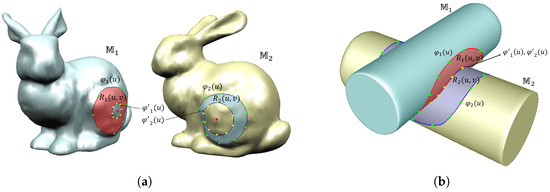
Figure 1. Blending regions of two meshes: (a) non-intersecting case and (b) intersecting case.

The main contributions of this paper are as follows:

• A method for automatically generating initial blending regions based on whether two meshes intersect, with the ability for users to interactively refine these regions directly on the mesh.
• A reparameterization strategy for establishing optimal curve correspondences, ensuring smooth and consistent blending surfaces without undesirable twisting.
• Flexible control over blending shapes, enabling the creation of complex blending meshes with high-order continuity.
• An extension of the proposed framework to consistently handle multiple intersection regions between meshes, enabling independent definition, control, and the seamless integration of each blending region into the final model.

The remainder of this paper is organized as follows. Section 2 reviews and analyzes previous studies on surface blending and blending techniques for triangular meshes. Section 3 describes the proposed method for generating blending regions using geodesic curves on meshes, adapting to intersection conditions. Section 4 details the construction of blending meshes, the reparameterization process for optimal curve correspondence, and the merging procedure with the input meshes. Section 5 presents experimental results, performance evaluations, and application examples. Section 6 concludes the paper.

2. Related Work

Blending techniques in geometric modeling, particularly those utilizing parametric surfaces, have been extensively reviewed and classified by Vida et al. [6]. These techniques are typically divided into parametric and implicit blending, with the former further categorized into rolling-ball blending, spine-based blending, and trimline-based blending. Among these, rolling-ball blending is a widely adopted approach in which a spherical cutter generates blending surfaces by traversing along adjacent surfaces. Methods proposed by Choi and Ju [7] and Farouki and Sverrisson [8] offer intuitive control over surface fullness; however, they are constrained by smoothness requirements and the need to avoid singularities in the offset surfaces. Sanglikar et al. [9] and Barnhill et al. [10] explored similar concepts, providing intuitive visualization but offering limited shape control and flexibility in defining blending regions.

Some of these limitations have been addressed through variable-radius rolling-ball methods. Chuang et al. [11,12] introduced a technique for deriving spine curves using variable radii. While this improves flexibility, the approach is computationally complex and imposes restrictions on the adaptability of contact curves. PDE-based blending techniques [13,14] can guarantee smooth continuity; however, they are also computationally intensive, limiting their practical use in interactive design scenarios. To balance geometric, technological, and aesthetic requirements, many studies have adopted parametric blending as a more practical alternative.

From the perspective of surface continuity and shape control, parametric blending offers considerable flexibility. Koparkar and Pramod [15] employed pointwise interpolation for blending surfaces and used reparameterized curves to minimize distortions. Li and Li [16] proposed blending bicubic B-spline patches, although their method is constrained by boundary conditions. Filip [17] and Kim et al. [18] utilized cubic Hermite interpolation to achieve $G^1$ continuity, while Elber [19] introduced a technique for blending arbitrary curves in functional designs. Despite their flexibility, these methods require complex tangent field computations, which reduce their efficiency in practice.

Linear interpolation provides a simpler yet effective alternative. Hartmann [1] generated $G^n$-continuous blending surfaces using parametric blending functions. Extending this concept, Song and Wang [2] produced blending surfaces by interpolating reparameterized surfaces and optimizing the resulting geometry by minimizing the strain energy. Hartmann [20] further extended the method to accommodate intersection curves. These approaches enable flexible blending regions, support higher-order continuity, and offer multiple design parameters for blend shape control. Building on this foundation, the present work adopts Hartmann’s linear interpolation method and extends it to polygonal meshes by directly defining and parameterizing free-form blending regions without mapping them to a 2D plane.

In the domain of polygonal models, setback vertex blending algorithms [21,22] and triangular Bézier surfaces [23] have been developed, and later extended to handle both vertices and edges efficiently [24]. However, these techniques remain limited in scope and often require complex, time-consuming preprocessing. To address such limitations, our approach defines and generates smooth blending regions directly on polygonal meshes, enabling the intuitive control of free-form blends without intricate preprocessing.

Blending techniques for triangular meshes have received comparatively less attention. Liu et al. [25] employed rolling-ball methods to blend intersecting meshes, but their approach struggled with complex geometries and provided limited shape control. Botsch et al. [26] introduced a resampling method to minimize normal noise and aliasing artifacts in blending regions, but it required significant user interaction. Lip and Yuen [27] blended meshes with NURBS surfaces using knot insertion to ensure boundary compatibility. Shin et al. [3] defined blending regions with boundary and auxiliary curves, parameterizing the local regions of two triangular meshes in geodesic polar coordinates. While effective, their approach lacked intuitive control for directly defining blending regions on the input meshes.

Applying parametric blending techniques to triangular meshes has typically required complex mesh parameterization methods [28,29,30,31,32,33], which transform local mesh regions into parametric surfaces. These procedures increase computational cost and reduce modeling flexibility. In contrast, the method proposed in this paper intuitively defines blending regions directly on meshes and transforms them into parametric surfaces, producing smooth and consistent blending surfaces through efficient geodesic-based operations and optimal curve reparameterization.

3. Construction of Blending Regions

This section describes the method for defining the blending regions $R_1(\subset {\mathbb{M}}_1)$ and $R_2(\subset {\mathbb{M}}_2)$ on the given triangular meshes ${\mathbb{M}}_1$ and ${\mathbb{M}}_2$, respectively. Each blending region is bounded by two closed geodesic Hermite spline curves [4] on the mesh. For $R_1$, the boundary is defined by the geodesic curves ${\phi }_1\left(u\right)$ and ${\phi }_1^{\prime }\left(u\right)$, and for $R_2$, by ${\phi }_2\left(u\right)$ and ${\phi }_2^{\prime }\left(u\right)$. We refer to ${\phi }_1\left(u\right)$ and ${\phi }_2\left(u\right)$ as the boundary curves, which serve as both the outer boundaries of the blending regions and the contact curves with the blending mesh. Similarly, ${\phi }_1^{\prime }\left(u\right)$ and ${\phi }_2^{\prime }\left(u\right)$ are referred to as the auxiliary curves, defining the inner boundaries of the blending regions.

Before constructing the blending regions, an intersection test is conducted to determine whether the input triangular meshes ${\mathbb{M}}_1$ and ${\mathbb{M}}_2$ intersect. Based on the test results, the procedure for generating the boundary and auxiliary curves is adapted to define appropriate blending regions, $R_1$ and $R_2$, on each mesh. This adaptive approach ensures that the blending regions are accurately positioned, enabling consistent and precise blending operations. Consequently, the resulting blending mesh provides a smooth and continuous connection between the two input meshes. The remainder of this section describes the methodology for constructing the blending regions in accordance with the intersection conditions, establishing a robust foundation for seamless blending across diverse geometric configurations.

3.1. Blending Region for Non-Intersecting Meshes

For two non-intersecting triangular meshes ${\mathbb{M}}_1$ and ${\mathbb{M}}_2$, the blending regions are defined by first locating two points, ${\mathbf{c}}_1$ and ${\mathbf{c}}_2$, representing the closest pair between the meshes. Around each point ${\mathbf{c}}_i$, n points are sampled such that each lies at a geodesic distance of $r_i$ from ${\mathbf{c}}_i$. Interpolating these sampled points yields closed geodesic Hermite spline curves, denoted by ${\phi }_i$, which form the outer boundaries of the blending regions. The auxiliary curves, ${\phi }_i^{\prime }$, are constructed in a similar manner by sampling n points at a geodesic distance of ${\alpha }_i{r}_i$ from ${\mathbf{c}}_i$, where ${\alpha }_i$ is a user-defined scaling factor controlling the relative position of the auxiliary boundary.

The parameters $r_i$ ($r_i>0$) and ${\alpha }_i$ ($0<{\alpha }_i<1$) are user-defined controls. The value of $r_i$ determines the overall size of the boundary curves; increasing $r_i$ proportionally enlarges the corresponding blending region. Similarly, ${\alpha }_i$ controls the relative position of the auxiliary curves with respect to ${\mathbf{c}}_i$: smaller values of ${\alpha }_i$ place the sampled interpolation points closer to the center, whereas larger values move them closer to the boundary curves. By adjusting $r_i$ and ${\alpha }_i$, users can precisely and intuitively control the extent and shape of the blending regions.

Figure 2 illustrates an example of blending regions generated using the proposed method. The red points on each mesh indicate the nearest points, ${\mathbf{c}}_1$ and ${\mathbf{c}}_2$, respectively. The green points on the curves represent the interpolation points for the boundary curves, while the yellow points indicate the interpolation points for the auxiliary curves. The blending region $R_1\subset {\mathbb{M}}_1$, defined by the geodesic curves ${\phi }_1\left(u\right)$ and ${\phi }_1^{\prime }\left(u\right)$, is shown in red, and the blending region $R_2\subset {\mathbb{M}}_2$, defined by ${\phi }_2\left(u\right)$ and ${\phi }_2^{\prime }\left(u\right)$, is shown in blue.

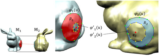
Figure 2. Blending regions $R_1$ and $R_2$ for two non-intersecting meshes.

Figure 2 presents an example of blending regions generated using the proposed method. On each mesh, the red points denote the closest pair of points, ${\mathbf{c}}_1$ and ${\mathbf{c}}_2$, respectively. Green points along the curves correspond to the interpolation points for the boundary curves, while yellow points indicate the interpolation points for the auxiliary curves. The blending region $R_1\subset {\mathbb{M}}_1$, bounded by the geodesic curves ${\phi }_1\left(u\right)$ and ${\phi }_1^{\prime }\left(u\right)$, is highlighted in red. Similarly, the blending region $R_2\subset {\mathbb{M}}_2$, bounded by ${\phi }_2\left(u\right)$ and ${\phi }_2^{\prime }\left(u\right)$, is highlighted in blue.

3.2. Blending Region for Intersecting Meshes

For intersecting meshes ${\mathbb{M}}_1$ and ${\mathbb{M}}_2$, the blending regions are defined with respect to the intersection polyline between the two meshes. This polyline is obtained by connecting intersection segments detected through a triangle–triangle intersection test. From the resulting intersection polyline, n points are uniformly sampled and interpolated to form a closed geodesic curve, which serves as the auxiliary curve ${\phi }_i^{\prime }$ for each mesh. By aligning the auxiliary curves with the intersection polyline, this approach provides a robust and geometrically consistent basis for defining the blending regions $R_1\subset {\mathbb{M}}_1$ and $R_2\subset {\mathbb{M}}_2$.

To define the boundary curves ${\phi }_i$ of the blending regions, offset polylines are generated by shifting the intersection polyline outward by a geodesic distance $r_i$ on each mesh. To prevent self-intersections of these offset polylines, a geodesic distance field-based technique is employed. Using Dijkstra’s algorithm, the geodesic distance $r_i$ from each point on the intersection polyline is computed, and points equidistant from the polyline are connected to form closed offset polylines [33]. Because this method uses unsigned geodesic distances, two offset polylines may be produced on the same mesh—one outside and one inside the intersection polyline. If an inner offset polyline were used as a boundary, it could generate an invalid blending region. Therefore, only the outward offset polyline is selected and used as the boundary curve.

Figure 3 illustrates the procedure for generating offset polylines in the correct outward direction. Starting from a point $\mathbf{p}$ on the intersection polyline, an outward vector ${\mathbf{d}}_i$ is defined reflecting the local geometric information of the opposite mesh (Figure 3a). For a triangle $T_1$ on mesh ${\mathbb{M}}_1$ containing $\mathbf{p}$, ${\mathbf{d}}_1$ is obtained by projecting the normal vector of the corresponding triangle $T_2$ (containing the corresponding point p) on ${\mathbb{M}}_2$ onto the plane of $T_1$ (Figure 3b). This projected vector ${\mathbf{d}}_1$ points outward from ${\mathbb{M}}_2$ and determines the correct offset direction for the boundary curve of $R_1$. An analogous process is used to compute ${\mathbf{d}}_2$ for ${\mathbb{M}}_2$.

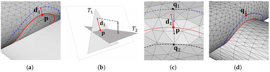
Figure 3. Offset process for boundary curve generation in blending regions: (a) definition of outward direction vector at intersection point, (b) projection of the opposite triangle normal to determine offset direction, (c) two candidate offset polylines (inner in black, outer in blue), and (d) final valid offset polyline used for boundary curve construction.

The unsigned geodesic distance may yield two candidate offset polylines (the inner one in black and the outer one in blue in Figure 3c). To determine the outer polyline, we evaluate

$$({\mathbf{q}}_k\ominus \mathbf{p})·{\mathbf{d}}_i>0,$$

(1)

where ${\mathbf{q}}_k$ is the closest point on each candidate polyline and ⊖ denotes the geodesic difference operator [4] from $\mathbf{p}$ to ${\mathbf{q}}_k$. The polyline containing the point ${\mathbf{q}}_k$ that satisfies this condition is selected as the outer polyline. Finally, the boundary curve ${\phi }_i$ for each mesh is constructed by interpolating n points uniformly sampled along the valid offset polyline.

As a result, this procedure produces robust blending regions $R_1$ and $R_2$ for intersecting meshes. Figure 4 shows an example generated using the proposed method, where the auxiliary curves are derived directly from the intersection polyline. Green points indicate the sampled points on the offset polylines, and yellow points mark the interpolation points of the auxiliary curves. The red region on ${\mathbb{M}}_1$, bounded by the geodesic curves ${\phi }_1\left(u\right)$ and ${\phi }_1^{\prime }\left(u\right)$, corresponds to $R_1$, while the blue region on ${\mathbb{M}}_2$, bounded by ${\phi }_2\left(u\right)$ and ${\phi }_2^{\prime }\left(u\right)$, corresponds to $R_2$.

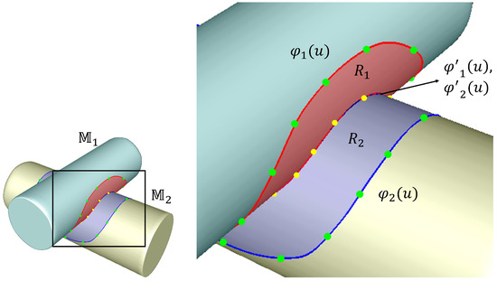
Figure 4. Blending regions $R_1$ and $R_2$ of two intersecting meshes.

By directing the offset curves outward from the intersection polyline and employing geodesic distance fields to prevent self-intersections, the proposed approach ensures that the resulting blending regions are smooth, well-defined, and suitable for subsequent blending operations.

4. Construction of Blending Mesh

A parametric blending surface is constructed by forming a linear combination of two parametric surfaces [1]. This process begins by transforming the blending regions $R_1\subset {\mathbb{M}}_1$ and $R_2\subset {\mathbb{M}}_2$ into their respective parametric forms, $R_i(u,v),i=1,2$. To avoid distortions and self-intersections in the resulting blending mesh, the boundary curves are reparameterized to establish an optimal correspondence, ensuring that the starting points are precisely aligned and the mapping along the curves remains consistent. This section details the parameterization of the blending regions and the reparameterization procedure used to produce a smooth, untwisted blending mesh.

4.1. Parametric Construction of Blending Mesh

To generate a parametric blending mesh that smoothly connects two blending regions, each region must first be represented in a parametric form. For this purpose, we define a function, denoted as glerp (geodesic linear interpolation), which computes a point on the mesh located at a geodesic fraction $v\in [0,1]$ between two given points $\mathbf{p}$ and $\mathbf{q}$:

$$glerp(v;\mathbf{p},\mathbf{q})=\mathbf{p}+vs.(\mathbf{q}\ominus \mathbf{p}),$$

(2)

where $(\mathbf{q}\ominus \mathbf{p})$ denotes the geodesic difference vector [4] from $\mathbf{p}$ to $\mathbf{q}$ on the mesh. This formulation ensures that interpolation is performed along the mesh surface rather than in Euclidean space, thereby preserving geometric fidelity in the blending process.

Using this function, the blending regions $R_1$ and $R_2$ can be expressed in parametric form as

$$\begin{array}{cc}\hfill R_1(u,v)& =glerp\left(v;{\phi }_1\left(u\right),{\phi }_1^{\prime }\left(u\right)\right),\hfill \\ \hfill R_2(u,v)& =glerp\left(v;{\phi }_2^{\prime }\left(u\right),{\phi }_2\left(u\right)\right),\hfill \end{array}$$

(3)

where $u,vs.\in [0,1]$. Here, $R_1(u,v)$ satisfies the boundary conditions $R_1(u,0)={\phi }_1\left(u\right)$ and $R_1(u,1)={\phi }_1^{\prime }\left(u\right)$, while $R_2(u,v)$ satisfies $R_2(u,0)={\phi }_2^{\prime }\left(u\right)$ and $R_2(u,1)={\phi }_2\left(u\right)$. This formulation enables blending regions of arbitrary shape to be systematically represented as explicit parametric forms, providing a consistent foundation for subsequent blending mesh construction.

Given the parametric regions $R_1(u,v)$ and $R_2(u,v)$, a $G^n$-continuous parametric blending mesh $S(u,v)$ can be constructed by linearly combining them using Hartmann’s blending function [1]:

$$S(u,v)=f_{n,\mu }\left(v\right)R_1(u,v)+\left(1-f_{n,\mu }\left(v\right)\right)R_2(u,v),$$

(4)

where $f_{n,\mu }\left(v\right)$ is a $G^n$-continuous blending function controlled by the parameters $\mu$ and n.

The blending function is given by

$$f_{n,\mu }\left(v\right)={\displaystyle \frac{\mu {(1-v)}^{n+1}}{\mu {(1-v)}^{n+1}+(1-\mu )v^{n+1}}},0<\mu <1,n\ge 0.$$

(5)

It has $C^n$ continuity and satisfies the boundary conditions

$$\begin{array}{cc}\hfill & f_{n,\mu }\left(0\right)=1,f_{n,\mu }\left(1\right)=0,\hfill \\ \hfill & f_{n,\mu }^{\left(k\right)}\left(0\right)=f_{n,\mu }^{\left(k\right)}\left(1\right)=0,k=1,\dots ,n,\hfill \end{array}$$

(6)

where $f_{n,\mu }^{\left(k\right)}$ denotes the kth derivative of $f_{n,\mu }$ with respect to v.

Figure 5a,b illustrate the blending function $f_{n,\mu }$ and its dependence on the shape-control parameters $\mu$ and n. The parameter $\mu$ adjusts the relative influence of $R_1$ and $R_2$: larger values bias the surface toward $R_1$, while smaller values emphasize $R_2$. The parameter n controls the smoothness of the transition, with larger values yielding higher-order continuity and smoother junctions at $v=0$ and $v=1$. Figure 5a and Figure 5b depict the effect of varying $\mu$ and n, respectively.

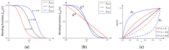
Figure 5. (a,b) Blending functions with varying control parameters; and (c) parameter transformation functions $p_1\left(v\right)$ and $p_2\left(v\right)$.

An additional control parameter $\lambda$ (referred to as the Thumb weight) is introduced via the parametric transformation functions $p_1\left(v\right)$ and $p_2\left(v\right)$, allowing the flexible adjustment of the blending surface shape. These functions are defined as

$$p_1\left(v\right)={\displaystyle \frac{v}{1-\lambda +\lambda v}}\mathrm{and}{p}_2\left(v\right)={\displaystyle \frac{v(1-\lambda )}{1-\lambda v}},0\le \lambda <1.$$

(7)

They satisfy the identity

$$p_2\left(v\right)=1-p_1(1-v).$$

(8)

This transformation modifies the influence of the auxiliary curves on the blending surface according to

$$S(u,v)=f_{n,\mu }\left(v\right)R_1\left(u,p_1\left(v\right)\right)+\left(1-f_{n,\mu }\left(v\right)\right)R_2\left(u,p_2\left(v\right)\right).$$

(9)

By adjusting $\lambda$, the fullness and curvature of the blending surface can be controlled, providing additional flexibility to meet specific design requirements. Figure 5c illustrates the graphs of $p_1\left(v\right)$ and $p_2\left(v\right)$ for varying values of $\lambda$.

4.2. Optimal Alignment of Boundary Curves

Establishing an optimal correspondence between the boundary curves is crucial to ensure a smooth and valid blending mesh [15]. An incorrect correspondence can lead to severe distortions in the resulting shape (Figure 6b,c, whereas a well-defined correspondence produces a smooth and consistent blending mesh (Figure 6a).

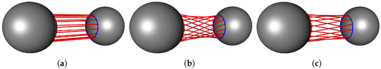
Figure 6. Examples of different correspondences between boundary curves and their resulting blending meshes: (a) correct correspondence, (b) incorrect correspondence (type 1), and (c) incorrect correspondence (type 2).

In this paper, we propose a method for establishing an optimal correspondence between boundary curves, regardless of whether curves are parameterized in the same or opposite directions, in order to generate a high-quality blending mesh. Following Lip et al. [27], the correspondence quality is quantitatively measured by the sum of the Euclidean distances between paired points on the two curves; a smaller sum indicates a better correspondence and typically yields a blending surface with minimal area.

Let ${\phi }_1\left(u_i\right)$ and ${\phi }_2\left(u_i\right)$, for $i=0,1,\dots ,m-1$, denote the m uniformly sampled points on each boundary curve. Since the curves are closed, sampling indices are treated with modulo m to ensure periodicity, i.e., ${\phi }_2\left(u_{(i\pm s)modm}\right)$ always refers to a valid point on the curve even after index shifting. To account for possible differences in curve orientation, we define two alignment functions:

$$D_F\left(s\right)=\sum _{i=0}^{m-1}∥{\phi }_1\left(u_i\right)-{\phi }_2\left(u_{(i+s)modm}\right)∥,s=0,1,\dots ,m-1,$$

(10)

$$D_B\left(s\right)=\sum _{i=0}^{m-1}∥{\phi }_1\left(u_i\right)-{\phi }_2\left(u_{(i-s)modm}\right)∥,s=0,1,\dots ,m-1,$$

(11)

where $\left|\right|·\left|\right|$ denotes the Euclidean distance in ${\mathbb{R}}^3$. Here, $D_F\left(s\right)$ represents the forward-shift alignment, which assumes that the two curves are parameterized in the same direction (e.g., clockwise–clockwise or counterclockwise–counterclockwise). Conversely, $D_B\left(s\right)$ represents the backward-shift alignment, which accounts for the case when the curves are parameterized in opposite directions (e.g., clockwise–counterclockwise). For each case, shift parameter s cyclically slides one curve against the other, and the total distance is computed for each alignment. Finally, the optimal alignment is determined by selecting the shift $s^{*}$ that minimizes the overall correspondence cost across both cases:

$$s^{*}=\left\{\begin{array}{cc}\underset{s}{argmin}{D}_F\left(s\right),\hfill & \mathrm{if}\underset{s}{min}{D}_F\left(s\right)<\underset{s}{min}{D}_B\left(s\right),\hfill \\ \underset{s}{argmin}{D}_B\left(s\right),\hfill & \mathrm{otherwise}.\hfill \end{array}\right.$$

This procedure ensures optimal correspondence between the two boundary curves, regardless of their parameterization direction. By considering all possible cyclic shifts, it remains robust to arbitrary starting points and minimizes the geometric discrepancy between paired points, resulting in a smoother and more consistent blending mesh. Using the optimal shift $s^{*}$, the correspondence between the parametric regions $R_1(u,v)$ and $R_2(u,v)$ can be expressed as

$$R_1(u,v)⟷R_2\left(\left(u\pm \frac{s^{*}}{m}\right)mod1,vs.\right),$$

where ± is chosen by the alignment that yields $s^{*}$: use + if $s^{*}\in arg{min}_s{D}_F\left(s\right)$, and − if $s^{*}\in arg{min}_s{D}_B\left(s\right)$.

4.3. Merging the Blending Mesh with Input Meshes

A blending mesh ${\mathbb{M}}_B$ is obtained by sampling the blending surface $S(u,v)$, thereby seamlessly connecting the two blending regions. This mesh is then merged with the input meshes ${\mathbb{M}}_1$ and ${\mathbb{M}}_2$ through a co-refinement step followed by trimming, resulting in a unified output mesh ${\mathbb{M}}_O$.

The co-refinement step ensures that ${\mathbb{M}}_B$ and the input meshes share common vertices and edges at corresponding positions. To achieve this, geodesic paths are constructed between adjacent sampling points along each boundary curve, and edge intersections along these paths are identified. Using these intersection points, the triangles in each mesh are subdivided so that their connectivity is mutually consistent.

Next, the trimming step removes all triangles within the regions enclosed by the boundary curves of the input meshes, producing a clean interface for merging. Finally, the boundary vertices and edges of ${\mathbb{M}}_B$ are connected to those of ${\mathbb{M}}_1$ and ${\mathbb{M}}_2$, completing the merge. Applying this procedure to both ${\mathbb{M}}_1$ and ${\mathbb{M}}_2$ yields the unified output mesh ${\mathbb{M}}_O$.

5. Experimental Results

The proposed parametric blending mesh generation technique for triangular meshes, based on geodesic interpolation curves, was implemented in C++ and tested on a PC equipped with an Intel(R) Core(TM) i7 2.50 GHz CPU, 32 GB of RAM, and an NVIDIA GeForce RTX 2060 GPU. The method automatically determines blending regions according to mesh intersection conditions and supports real-time user interaction. In addition, it provides intuitive control over the blending mesh shape via user-defined parameters, while ensuring seamless connectivity between the blending mesh and the input meshes. These capabilities make the method applicable to a wide range of modeling and design scenarios. This section presents experimental results demonstrating the efficiency and versatility of the proposed technique through examples of blending regions and resulting meshes generated from various 3D triangular mesh inputs.

5.1. Control Parameters for Blending Shapes

The parameters $r_i$ ($i=1,2$) and ${\alpha }_i$ are key shape-control factors: $r_i$ determines the overall extent of the blending region, while ${\alpha }_i$ adjusts the position of the auxiliary curve relative to the boundary curve. Figure 7 presents the blending results for two sphere models with varying values of $r_i$ and ${\alpha }_i$. Figure 7a shows two blending regions and their corresponding blending meshes generated with different $r_i$ values; as $r_i$ increases, the blending region expands. In contrast, Figure 7b illustrates blending regions and meshes generated with the same $r_i$ but different ${\alpha }_i$ values. Increasing ${\alpha }_i$ moves the auxiliary curve closer to the boundary curve, reducing the blending region’s area and causing the resulting blending mesh to more strongly reflect the boundary curve’s geometry.

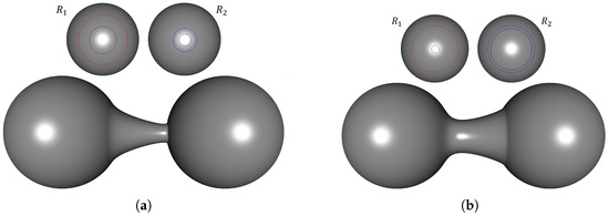
Figure 7. Blending meshes generated with user-defined parameters $r_i$ and ${\alpha }_i$: (a) $r_1=3.0$, $r_2=1.0$, ${\alpha }_1={\alpha }_2=0.5$; and (b) $r_1=r_2=3.0$, ${\alpha }_1=0.15$, ${\alpha }_2=0.85$.

Figure 8a shows examples of blending meshes generated for complex regions defined by geodesic interpolation curves. Users can interactively adjust the boundary curves in real time by manipulating the interpolation points directly on the mesh. In each example, the upper row presents the defined blending regions, while the lower row displays the corresponding blending meshes that seamlessly connect these regions. Furthermore, Figure 8b illustrates the connection between the blending mesh and the two input sphere meshes. These results demonstrate that the proposed method preserves geometric consistency, even for blending regions with complex shapes.

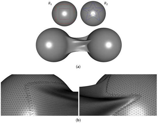
Figure 8. Blending meshes generated from user-defined blending regions: (a) blending meshes created from rectangular and star-shaped regions; and (b) junction between the blending mesh and two input meshes.

Figure 9 presents the blending meshes for two models with identical blending regions but different values of $\mu$ in the blending function $f_{n,\mu }$, which controls the relative influence of the two regions $R_1$ and $R_2$. When $\mu$ is close to 0, the blending mesh more closely follows the shape of $R_2$, whereas when $\mu$ is close to 1, it increasingly reflects the geometry of $R_1$. This parameter allows smooth and flexible control over the transition between the two regions.

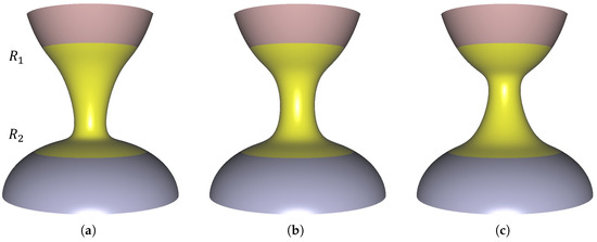
Figure 9. Blending the results of two sphere meshes with a varying balance parameter $\mu$: (a) $\mu =0.1$; (b) $\mu =0.5$; (c) $\mu =0.9$.

Figure 10a–c illustrate the influence of the parameter n in the blending function $f_{n,\mu }$ on the blending results between the sphere and the box, while Figure 10d–f depict the gradient fields of the blending mesh. As n increases, the blending mesh achieves higher-order continuity, leading to smoother and more coherent transitions between the two models. We compute the gradient of the scalar function, where the scalar value assigned to each vertex is the mean curvature, by assuming piecewise linear interpolation over each triangular face. For each face, the gradient is evaluated using the vertex values and the face geometry, resulting in a piecewise constant gradient field across the mesh. The appropriate continuity order, however, depends on the target application.

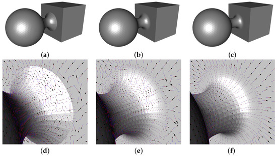
Figure 10. Blending results for the sphere–box model and corresponding scalar field gradients with the varying continuity parameter n: (a,d) $G^0$; (b,e) $G^1$; (c,f) $G^2$.

For example, $G^0$ continuity may be sufficient in tasks requiring only geometric connectivity, such as volumetric analysis or collision detection, even though visible creases remain along the interface. $G^1$ continuity ensures tangent alignment, producing visually smoother transitions. It is well suited for interactive visualization or real-time rendering, where efficiency is prioritized over curvature smoothness. In contrast, $G^2$ continuity guarantees curvature consistency, eliminating highlight discontinuities and ensuring seamless surface quality. This level of smoothness is essential in advanced design and manufacturing, for instance, in automotive panels or biomedical implants, where both aesthetics and manufacturability critically depend on curvature continuity.

In addition to geometric appearance, continuity differences are also evident in the gradient fields. With $G^0$ continuity (Figure 10d), the blending mesh exhibits discontinuities not only along the boundary curve but also across the surface, resulting in an unstable gradient field. With $G^1$ continuity (Figure 10e), the transition near the boundary becomes smoother and the gradient field is continuous at the junction, but instabilities appear farther away. In contrast, $G^2$ continuity (Figure 10f) provides a globally continuous and stable gradient field across the entire blending mesh.

Figure 11 presents the blending results for a cylinder–box pair with varying values of $\lambda$ (Thumb weight), which controls the degree to which the blending mesh conforms to the auxiliary curves. As $\lambda$ approaches 1, the mesh aligns more closely with these curves, affecting the fullness of the shape and providing designers with finer control to meet specific aesthetic or functional requirements.

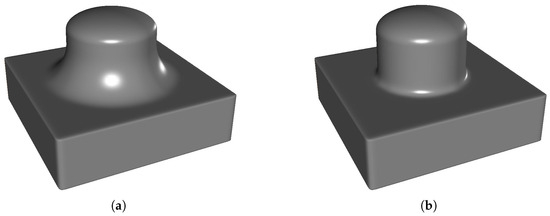
Figure 11. Blending meshes of the intersection region with varying thumb weight $\lambda$: (a) $\lambda =0$; (b) $\lambda =0.9$.

5.2. Performance Analysis of Mesh Blending

This section reports the computation time of the proposed method for both non-intersecting and intersecting mesh cases, along with a visual inspection of the results. Figure 12 and Figure 13 present blending results for various models, including primitive shapes (e.g., cylinder, box, torus, sphere) and scanned datasets (e.g., Bunny, teeth).

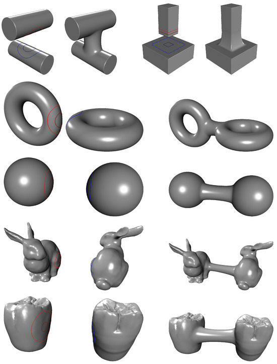
Figure 12. Example of blending between non-intersecting meshes.

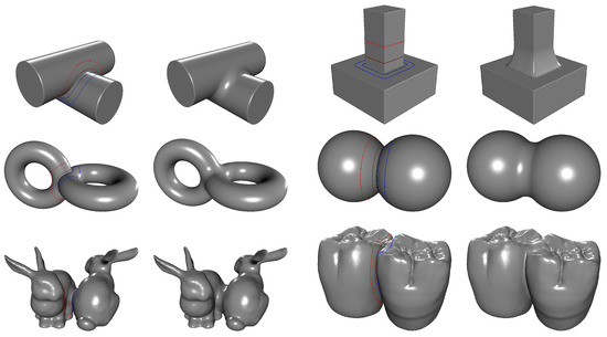
Figure 13. Example of blending between intersecting meshes.

Table 1 presents detailed information about each model, including the total number of triangles, the number of triangles contained within the blending region, and the computation time required for each stage of the blending process. As observed, the total computation time for blending non-intersecting meshes tends to increase with the number of triangles in the blending region, with the blending region construction stage accounting for an increasingly significant portion of the total time.

Table 1. Computation time (in ms) for blending between non-intersecting meshes.

Models		Cylinder	Torus	Box	Sphere	Bunny	Tooth
# of faces		1632	2842	3072	5120	16,650	40,958
# of faces in blending region		362	390	534	745	1054	6024
Time (ms)	Intersection check	1	2	2	4	13	32
	Blending region construction	23	29	30	77	235	1270
	Blending mesh construction	47	50	69	71	87	182
	Merging	17	25	26	35	107	235
	Total	88	106	129	186	442	1719

Table 2 presents the performance metrics for blending intersecting meshes, including the number of triangles in the blending regions, the number of intersection points along the polyline, and the computation time at each processing stage. Similarly to the non-intersecting case, the total computation time increases as the number of triangles in the blending region grows. In addition, the number of intersection points substantially affects the computation of geodesic offset curves, leading to longer times for constructing the blending region.

Table 2. Computation time (in ms) for blending between intersecting meshes.

Models		Cylinder	Torus	Box	Sphere	Bunny	Tooth
# of faces in region		580	646	906	1024	2044	5123
# of intersection points		221	153	165	207	207	606
Time (ms)	Intersection check	1	2	2	4	13	32
	Blending region construction	49	32	37	51	55	144
	Blending mesh construction	104	108	110	131	159	369
	Merging	27	33	34	52	177	393
	Total	181	175	183	238	404	938

As a result, the most time-consuming stage in the proposed blending framework is the construction of the blending region, particularly the computation of the geodesic distance field initiated from a seed point or a closed polyline. The distance field was generated using a distance propagation algorithm [33] within the local blending region, and its computational complexity can be expressed as $O(nlogn)$, where n denotes the number of vertices in the blending region. For non-intersecting meshes, the blending region is constructed from a single seed point with complexity $O(nlogn)$. In contrast, for intersecting meshes, geodesic distance fields must be computed from each of the m intersection points located on the intersection polyline, resulting in an overall complexity of $O(mnlogn)$. This implies that the computational cost of blending region construction scales linearly with the number of intersection points m, which is consistent with our experimental observations listed in Table 1 and Table 2.

To evaluate the convergence behavior of the proposed parametric blending method, we performed an experimental study based on the sampling resolution of the generated blending meshes. Specifically, a reference surface with resolution of $30\times 30$ in the parametric domain was selected, and blending surfaces with higher resolutions (from $40\times 40$ up to $300\times 300$) were compared against it. The geometric errors were quantified using symmetric mean, root-mean-square (RMS), and maximum point-to-surface distances.

As shown in Figure 14, the mean distance (in blue) decreases from 0.1258 at $40\times 40$ to approximately 0.08 at higher resolutions. Similarly, the RMS distance (in yellow) decreases from 0.1419 to around 0.09. After approximately $60\times 60$, both mean and RMS distances remain nearly constant, regardless of further refinement, while the maximum error stays relatively stable around 0.30. At integer multiples of the reference resolution (e.g., $90\times 90$, $150\times 150$, $210\times 210$), the error values drop more noticeably. This alignment effect occurs because the sampling grids become better synchronized with the reference grid, thereby reducing point-to-surface errors. These results indicate that the proposed blending method demonstrates experimental convergence with respect to sampling resolution: as the resolution increases, the error rapidly decreases and then stabilizes at consistent values. This confirms that stable and accurate blending surfaces can be achieved even at moderate resolutions. As a limitation, however, it should be noted that this convergence analysis is based on experimental sampling resolution rather than a formal theoretical proof.

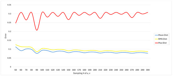
Figure 14. Symmetric convergence analysis of the proposed parametric blending method under different sampling resolutions: mean distance (blue), RMS distance (yellow), and maximum distance (red).

5.3. Comparison with Existing Approaches

In this subsection, we evaluate the proposed parametric blending method through a comparative study with representative existing approaches. Specifically, we consider the parametric blending technique of Shin et al. [3], which is based on geodesic polar coordinates, and the signed distance field (SDF)-based smooth union [34]. For comparison, sphere and torus models are employed to investigate both non-intersecting and intersecting cases. The blending results are compared in terms of controllability and geometric fidelity providing insights into the strengths and limitations of each approach.

As shown in Figure 15, the result on the left, generated by Shin et al.’s method, does not consider the optimal alignment of boundary curves, leading to a twisted blending mesh. In contrast, the result on the right, obtained by our method, incorporates optimal alignment, resulting in well-aligned iso-parametric curves and demonstrating the stability and effectiveness of the proposed approach. Moreover, our method enables the direct control of the boundary curves, whereas Shin et al.’s method offers only indirect control in the parametric space, which is less intuitive. In addition, the proposed method is capable of handling cases with multiple intersections between meshes, while Shin et al.’s method cannot deal with intersecting cases at all.

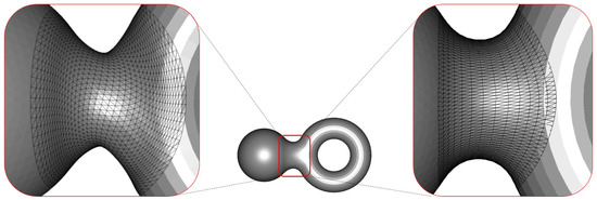
Figure 15. Comparison of blending meshes: without optimal alignment (Shin et al.’s method [3], left) vs. with optimal alignment (proposed method, right).

The smooth union can be regarded as a smooth variant of the classical Boolean union operation, and has been widely adopted as a fundamental blending operator for implicit surfaces. When the two models are in close proximity, the smooth union can generate a blended result. In the experiments, the smooth union was implemented using the smooth minimum function of a quadratic polynomial proposed by [34]

$$\mathrm{smin}(a,b,k)=min(a,b)-{\displaystyle \frac{{\left(max(0,k-|a-b\left|\right)\right)}^2}{4k}},$$

(12)

where k controls the thickness of the blending region.

Figure 16 shows the blending results of the SDF-based smooth union for spheres and tori at different distances with the control parameter $k=1$. As can be observed, a blended connection is formed only when the two models are within a certain distance threshold determined by k, while no blending occurs once the separation exceeds this range. In contrast, the proposed method can generate blending meshes that connect two objects regardless of their distance. Furthermore, whereas the smooth union provides only a single control parameter, our method offers multiple parameters such as n, $\mu$, and $\lambda$, enabling the more versatile adjustment of the blending surface, as demonstrated in Section 5.1.

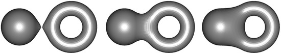
Figure 16. Results of the smooth union of spheres and tori at different distances ($k=1$).

It should also be noted that the SDF-based smooth union performs blending through a simple minimum operation on the distance fields, which makes it highly efficient. However, the result must be converted back to a mesh representation using algorithms such as marching cubes, which can lead to changes in the geometric characteristics of the mesh, including the number of vertices and connectivity. Finally, Table 3 summarizes the characteristics of the three approaches—Shin et al.’s method, the SDF-based smooth union, and our proposed method—highlighting their respective strengths and limitations.

Table 3. Comparison of existing blending methods and the proposed method.

Evaluation Criteria	Smooth Union [34]	Shin et al. [3]	Proposed Method
Blending boundary control	No	Partial	Yes
Multiple control parameters	No	Yes	Yes
Continuity control	No	Yes	Yes
Optimal alignment of boundary curves	Yes	No	Yes
Preservation of input mesh structure	No	Yes	Yes
Support for multiple intersections	Yes	No	Yes
Support for multiple mesh blending	Yes	No	No
Computational efficiency	High	Medium	Moderate

5.4. Applications

The proposed mesh blending technique provides an efficient, intuitive, and robust solution for mesh modeling, enabling smooth transitions between input meshes and offering broad applicability across diverse scenarios.

A key advantage of the method is its ability to process multiple intersection regions simultaneously. When two meshes intersect at several locations, the algorithm identifies each intersection separately and constructs an independent blending region for it. Figure 17 demonstrates this capability using a long cylindrical model and a hollow cylindrical model intersecting at four distinct regions. For each intersection, a dedicated blending region is defined, a corresponding blending mesh is generated, and the result is seamlessly merged into the final model. Furthermore, the method allows for independent control over the shape and width of each blending region, ensuring precise and natural transitions even for complex intersection curves.

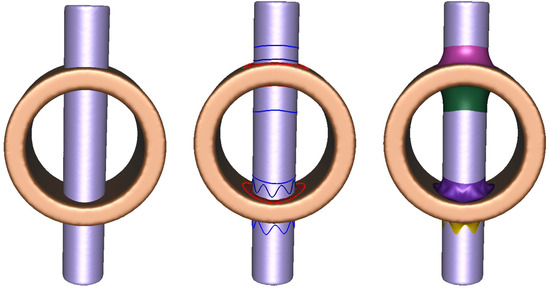
Figure 17. Blending process for meshes with multiple intersections.

In addition to processing multiple intersections, the proposed technique can also successively blend multiple meshes into a single unified model. This is achieved through a consistent blending process that operates effectively regardless of the presence or absence of intersections. Figure 18 demonstrates this capability by sequentially blending three cylindrical models—both non-intersecting and intersecting—into a unified mesh with smooth, continuous transitions.

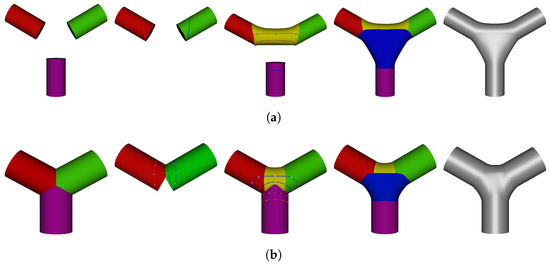
Figure 18. The successive blending of three cylindrical models to form a unified mesh: (a) non-intersecting case; and (b) intersecting case.

To further highlight its practical applicability, Figure 19 shows a 3D-printed model derived from the blending mesh in Figure 18b. The printed model exhibits seamless, well-integrated transitions between parts, demonstrating the potential of the proposed technique for designing and manufacturing mechanical components. Such smooth surface continuity is often critical in fabrication, and the method’s intuitive region specification and versatile shape-control parameters make it well-suited to meeting these requirements.

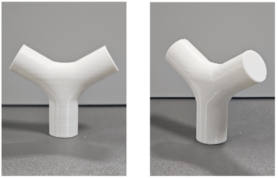
Figure 19. Three-dimensional-printed result of the blending mesh.

In addition to its practical value in fabrication, the proposed method shows strong potential for aesthetic and design-oriented applications. It preserves the original mesh geometry and fine details while enabling intuitive adjustments to curvature, width, and overall shape. These capabilities are particularly advantageous in digital content creation, such as 3D modeling and visual design. Figure 20 presents an example where multiple meshes are seamlessly blended into a single cohesive structure. The resulting mesh exhibits smooth, continuous transitions with no noticeable artifacts or geometric distortions.

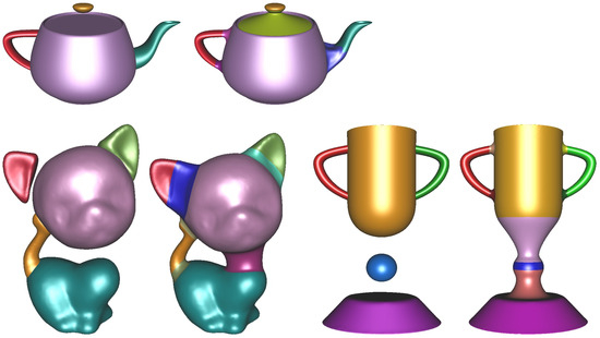
Figure 20. Results of blending multiple meshes.

Figure 21 presents examples of high-resolution and high-curvature meshes commonly used in digital content production. The results demonstrate that the proposed method successfully preserves and smoothly transitions the fine details and complex geometrical features of the original meshes. This confirms the effectiveness of the method not only for simple shapes but also for complex models frequently encountered in practical applications.

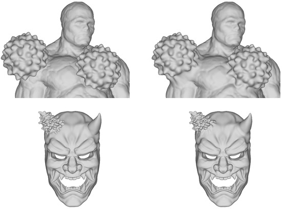
Figure 21. Blending results of blending high-resolution and high-curvature meshes.

6. Conclusions

This paper has presented a robust and flexible method for defining free-form blending regions between two triangular meshes and generating the smooth blending meshes that seamlessly connect them. The blending regions are defined using geodesic interpolation curves, derived from either minimum-distance point pairs or intersection curves, depending on whether the input meshes intersect. Each region is parameterized as a surface via geodesic linear interpolation, and a $G^n$-continuous blending function is applied to generate the final blended mesh. To improve the quality and ensure geometric consistency, an optimal boundary-curve correspondence is established through re-parameterization and distortion minimization. An additional parametric transformation with a Thumb weight parameter further enhances user control over the fullness and curvature of the blending mesh. Finally, a co-refinement, trimming, and merging process integrates the blending mesh with the input meshes, producing a unified mesh with consistent connectivity.

The proposed framework supports both intersecting and non-intersecting cases, provides intuitive real-time control over blending shapes, and preserves the key geometric characteristics of the input models. Experimental results across a range of complex mesh configurations have demonstrated its robustness, versatility, and suitability for various applications. In addition, comparative experiments with representative existing approaches, including the parametric blending method [3] and the SDF-based smooth union [34], have shown the superior controllability and geometric fidelity of the proposed method.

Nevertheless, the current framework is limited to blending between two meshes and cannot be directly applied to scenarios where multiple meshes intersect simultaneously. Moreover, while extensive performance evaluation, complexity analysis, and convergence studies were conducted, these quantitative assessments have primarily focused on computational efficiency and visual quality. A comprehensive quantitative comparison with state-of-the-art techniques (e.g., neural network-based or voxel-based approaches) is not supported by the current framework, as it is primarily designed to emphasize geometric fidelity and controllability. In contrast, voxel-based methods inherently exhibit properties such as conservativeness, rigidity, and locality due to their volumetric field formulation. As a result, direct comparison across these heterogeneous representations is inherently difficult and remains a challenging research problem.

Future research will therefore focus on extending the proposed method to support the simultaneous blending of multiple meshes, as well as developing unified metrics that enable fair quantitative comparison with fundamentally different approaches such as voxel-based or neural network–based methods. These efforts will facilitate more direct evaluation against state-of-the-art techniques and ultimately contribute to a more general and scalable blending framework. The video demonstration is available at https://youtu.be/R4E6F88ApCI?si=FVBQFe22kGztu2Mv (accessed on 29 September 2025).

References

- Hartmann, E. Parametric Gn blending of curves and surfaces blending functions. Vis. Comput. VC 2001, 17, 1–13. [Google Scholar] [CrossRef]
- Song, Q.; Wang, J. Generating Gn parametric blending surfaces based on partial reparameterization of base surfaces. Comput.-Aided Des. 2007, 39, 953–963. [Google Scholar] [CrossRef]
- Shin, M.C.; Hwang, H.D.; Yoon, S.H.; Lee, J. Parametric blending of triangular meshes. Symmetry 2018, 10, 620. [Google Scholar] [CrossRef]
- Ha, Y.; Park, J.H.; Yoon, S.H. Geodesic Hermite spline curve on triangular meshes. Symmetry 2021, 13, 1936. [Google Scholar] [CrossRef]
- Polthier, K.; Schmies, M. Straightest geodesics on polyhedral surfaces. In Proceedings of the ACM SIGGRAPH 2006 Courses, New York, NY, USA, 30 July 2006; SIGGRAPH ’06. pp. 30–38. [Google Scholar]
- Vida, J.; Martin, R.R.; Varady, T. A survey of blending methods that use parametric surfaces. Comput.-Aided Des. 1994, 26, 341–365. [Google Scholar] [CrossRef]
- Choi, B.; Ju, S. Constant-radius blending in surface modelling. Comput.-Aided Des. 1989, 21, 213–220. [Google Scholar] [CrossRef]
- Farouki, R.A.; Sverrisson, R. Approximation of rolling-ball blends for free-form parametric surfaces. Comput.-Aided Des. 1996, 28, 871–878. [Google Scholar] [CrossRef]
- Sanglikar, M.; Koparkar, P.; Joshi, V. Modelling rolling ball blends for computer aided geometric design. Comput. Aided Geom. Des. 1990, 7, 399–414. [Google Scholar] [CrossRef]
- Barnhill, R.E.; Farin, G.E.; Chen, Q. Constant-radius blending of parametric surfaces. In Geometric Modelling; Springer: Vienna, Austria, 1993; pp. 1–20. [Google Scholar]
- Chuang, J.H.; Lin, C.H.; Hwang, W.C. Variable-radius blending of parametric surfaces. Vis. Comput. 1995, 11, 513–525. [Google Scholar] [CrossRef]
- Chuang, J.H.; Hwang, W.C. Variable-radius blending by constrained spine generation. Vis. Comput. 1997, 13, 316–329. [Google Scholar] [CrossRef]
- Bloor, M.I.G.; Wilson, M.J. Generating blend surfaces using partial differential equations. Comput.-Aided Des. 1989, 21, 165–171. [Google Scholar] [CrossRef]
- Bloor, M.I.G.; Wilson, M.J. Using partial differential equations to generating freeform surfaces. Comput.-Aided Des. 1990, 22, 221–234. [Google Scholar] [CrossRef]
- Koparkar, P. Parametric blending using fanout surfaces. In Proceedings of the First ACM Symposium on SOLID Modeling Foundations and CAD/CAM Applications, Austin, TX, USA, 5–7 June 1991; pp. 317–327. [Google Scholar]
- Li, G.; Li, H. Blending parametric patches with subdivision surfaces. J. Comput. Sci. Technol. 2002, 17, 498–506. [Google Scholar] [CrossRef]
- Filip, D.J. Blending parametric surfaces. ACM Trans. Graph. 1989, 8, 164–173. [Google Scholar] [CrossRef]
- KIM, K.; ELBER, G. A symbolic approach to freeform parametric surface blends. J. Vis. Comput. Animat. 1997, 8, 69–80. [Google Scholar] [CrossRef]
- Elber, G. Generalized filleting and blending operations toward functional and decorative applications. Graph. Model. 2005, 67, 189–203. [Google Scholar] [CrossRef]
- Hartmann, E. Gn blending with rolling ball contact curves. In Proceedings of the Geometric Modeling and Processing 2000, Theory and Applications, Hong Kong, China, 10–12 April 2000; pp. 385–389. [Google Scholar]
- Terék, Z.; Várady, T. Setback vertex blends in digital shape reconstruction. In Mathematics of Surfaces XIII; Springer: Berlin/Heidelberg, Germany, 2009; pp. 356–374. [Google Scholar]
- Zhou, P.; Qian, W.H. Polyhedral vertex blending with setbacks using rational S-patches. Comput. Aided Geom. Des. 2010, 27, 233–244. [Google Scholar] [CrossRef]
- Zhou, P.; Qian, W.H. A vertex-first parametric algorithm for polyhedron blending. Comput.-Aided Des. 2009, 41, 812–824. [Google Scholar] [CrossRef]
- Zhou, P.; Qian, W.H. Blending polyhedral edge clusters. In Image and Graphics; Springer: Cham, Switzerland, 2019; pp. 193–207. [Google Scholar]
- Liu, Y.S.; Zhang, H.; Yong, J.H.; Yu, P.Q.; Sun, J.G. Mesh blending. Vis. Comput. 2005, 21, 915–927. [Google Scholar] [CrossRef]
- Botsch, M.; Kobbelt, L. Resampling feature and blend regions in polygonal meshes for surface anti-aliasing. Comput. Graph. Forum 2001, 20, 402–410. [Google Scholar] [CrossRef]
- Lai, L.M.; Yuen, M.M. Blending of mesh objects to parametric surface. Comput. Graph. 2015, 46, 283–293. [Google Scholar] [CrossRef]
- Floater, M.S. Parametrization and smooth approximation of surface triangulations. Comput. Aided Geom. Des. 1997, 14, 231–250. [Google Scholar] [CrossRef]
- Gu, X.; Yau, S.T. Global conformal surface parameterization. In Proceedings of the Eurographics Symposium on Geometry Processing, Aachen, Germany, 23–25 June 2003. [Google Scholar]
- Floater, M.S.; Hormann, K. Surface parameterization: A tutorial and survey. In Advances in Multiresolution for Geometric Modelling; Springer: Berlin/Heidelberg, Germany, 2005; pp. 157–186. [Google Scholar]
- Sheffer, A.; Praun, E.; Rose, K. Mesh parameterization methods and their applications. Found. Trends. Comput. Graph. Vis. 2006, 2, 105–171. [Google Scholar] [CrossRef]
- Jin, M.; Kim, J.; Luo, F.; Gu, X. Discrete surface Ricci flow. IEEE Trans. Vis. Comput. Graph. 2008, 14, 1030–1043. [Google Scholar] [CrossRef]
- Melvær, E.L.; Reimers, M. Geodesic polar coordinates on polygonal meshes. Comput. Graph. Forum 2012, 31, 2423–2435. [Google Scholar] [CrossRef]
- Quilez, I. Smooth Minimum. 2013. Available online: https://iquilezles.org/articles/smin/ (accessed on 29 September 2025).
Disclaimer/Publisher’s Note: The statements, opinions and data contained in all publications are solely those of the individual author(s) and contributor(s) and not of MDPI and/or the editor(s). MDPI and/or the editor(s) disclaim responsibility for any injury to people or property resulting from any ideas, methods, instructions or products referred to in the content. |
© 2025 by the authors. Licensee MDPI, Basel, Switzerland. This article is an open access article distributed under the terms and conditions of the Creative Commons Attribution (CC BY) license (https://creativecommons.org/licenses/by/4.0/).