Abstract
In this paper we propose a statistical model that combines both autoregressions and fractional differentiation in a unified treatment. However, instead of imposing that the roots are strictly on the unit circle, we also allow them to be within the unit circle. This permits a higher degree of flexibility in the specification of the model, with rates of dependence combining exponential with hyperbolic decays. Monte Carlo experiments and empirical applications to climatological and financial data show that the proposed approach performs well.
MSC:
62M10
1. Introduction
This paper puts forward a general statistical model in the time domain based on the concept of fractional integration [] ore specifically, in the proposed framework, instead of imposing that the roots are strictly on the unit circle, as is the case with unit root models and purely fractional integration approaches, we also allow them to be within the unit circle. The reason for this is that a fractional root can be any real number, and therefore may or may not lie on the unit circle, which contains only complex numbers with a magnitude (or modulus) of 1 [,]. This approach enables us to specify the time series in terms of its infinite past, with a rate of dependence between the observations much smaller than that produced by the classic I(d) representations. In particular, we consider processes of the following form:
with |α| < 1 and d > 0. For simplicity, we assume that ut is i.i.d. Clearly, if α = 1 in (1), xt is I(d) and exhibits long memory since d > 0 []. However, if |α| < 1, the process is no longer characterized by long memory, although xt will still be a function of its infinite past as long as d is a real value. Thus, the main contribution of this work is the specification of a novel model that combines both autoregressions with fractional differentiation in a single framework; however, instead of considering a fractional process with autoregressive disturbances (e.g., as in []), we incorporate the autoregression in the fractional polynomial. In doing so, we allow for a more flexible specification of the model, incorporating stationary and nonstationary structures with different degrees of dependence across time.
The remainder of the paper is organized as follows: Section 2 describes the time series model; Section 3 presents a procedure for simultaneously testing the two parameters, d and α, in (1); Section 4 reports on various Monte Carlo experiments; Section 5 discusses some empirical applications to show the usefulness of the proposed approach; and Section 6 offers some concluding remarks. Additional technical details are provided in the Appendix A and Appendix B.
2. The Statistical Model
The starting point is the model given by (1). As already mentioned, if α = 1, the polynomial in (1) is exactly on the unit circle, and xt is said to be integrated of order d, denoted by xt~I(d). Note that given that d > 0, the polynomial (1 − L)d can be expressed in terms of its Binomial expansion, such that, for all real values of d,
These processes (of the form (1 − L)d xt = ut) were introduced by [,,], and they have been widely employed in the time series literature [,]. A useful survey of I(d) statistical models can be found in Baillie (1996) [], and reviews of the relevant theoretical and applied issues can be found in [] and, more recently, in [].
For the purpose of the present paper, we define long memory as a process whose spectral density function, f(λ), tends to infinity as λ approximates 0, i.e.,
In the case of α = 1, the spectral density function of xt is:
where σ2 = Var(ut), implying that at λ = 0, the spectral density function is unbounded for d > 0. However, if |α| < 1, then
which is bounded for all α ≠ 1, and thus, in this case (|α| < 1), the process is stationary for all real values of d. If d is an integer value, xt will be a function of a finite number of lag values of xt; that is, xt is an AR(d) process in this case. However, if d is a real number, one can still use the Binomial expansion, such that
and xt in (1) will be a function of its infinite past.
Note that, using (5), (1) can be written as:
with
which is an AR(∞) process. Similarly, (1) can also be expressed as
and again using the standard Binomial expansion:
where Γ(x) stands for the Gamma function. It follows that
Thus, xt also admits a MA(∞) representation.
Figure 1 displays the region of (α, d)-values for the interval (0, 2). It can be seen that the process considered is stationary for all values of α < 1. Also, if α = 1 and d < 0.5, xt is stationary, while it is not for the remaining values of these parameters. Note that if α > 1, the process is explosive. Concerning the stationary region, as d moves from 0 towards 1, and α from 0 to higher values, the dependence between the observations becomes higher. In fact, one of the advantages of this approach is that it allows for a higher degree of flexibility in the dynamic specification of the model, avoiding the rigidities caused by the exponential decay of the autoregressive part and the hyperbolically slower one produced by the fractional differencing part.
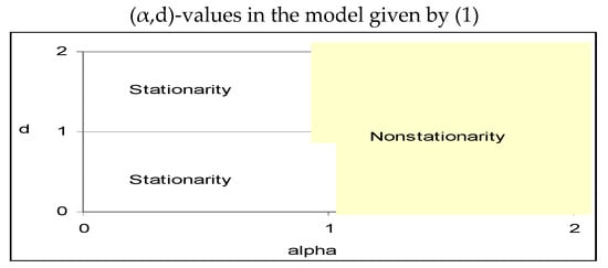
Figure 1.
Stationary/nonstationary (α,d) region in Equation (1).
Figure 2 displays plots of simple realizations of processes of the form given by (1) for different values of α and d and T = 100. The plots on the left-hand-side of the figure correspond to the case of long memory (α = 1), while those on the right-hand-side correspond to short memory, with α = 0.80. In all cases we take d = 0.35, 0.75 and 1. In particular, the upper-left plot corresponds to the case with d = 1 and α = 0.35, namely to an I(0.35) process, which exhibits long memory despite being stationary; by contrast, in the two plots below (I(0.75) and I(1)), the processes are clearly nonstationary. Finally, stationarity is found in all cases when α = 0.80.
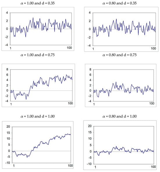
Figure 2.
Simple realizations of models of the form (1 − αL)dxt = εt. The plots are sample realizations of the model in Equation (1) for a range of values for α and d.
Figure 3 displays the first 50 sample autocorrelation values of the realizations in Figure 2. It can be seen that in the long memory cases these decay at a hyperbolic rate, and in the short memory case the rate of decay slows down as d increases. Figure 4 displays the periodograms, with higher peaks corresponding to lower frequencies in the long memory cases.
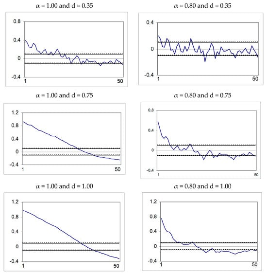
Figure 3.
Correlograms of the realizations in Figure 2. The large-sample standard error under the null hypothesis of no autocorrelation is 1/√T.
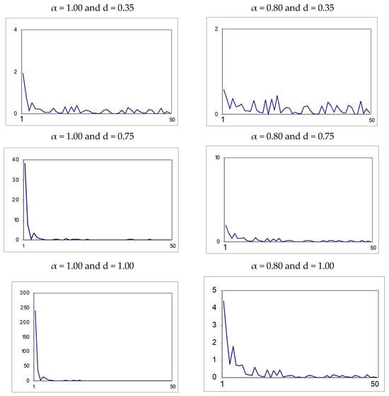
Figure 4.
Periodograms of the realizations in Figure 2. The periodograms were computed on the basis of the discrete Fourier frequencies λj = 2πj/T.
Figure 5 displays the impulse response functions obtained from the coefficients of the infinite MA representation in (7). As expected, mean reversion occurs in all cases except when α = d = 1 (the random walk model). These values correspond to the coefficients bj in the MA(∞) representation of xt in (7). This figure shows that when increasing α and d, the impulse responses have a longer time horizon before disappearing completely.
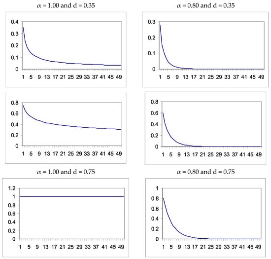
Figure 5.
Impulse response functions of the realizations in Figure 2. The values indicate the impulse responses based on the coefficients of the MA(∞) representation of the series given by Equation (7).
3. The Testing Procedure
In this section we develop a score test of the null hypothesis:
in the model given by (1) for any real values do > 0 and |αo| < 1, under the assumption that ut in (1) is a sequence of zero-mean uncorrelated random variables with unknown variance σ2.
Specifically, the score statistic for Ho in (8) is constructed as follows. Consider a column vector of parameters η = (α, d, σ2)’ and let L(η) be an objective function, such as the negative of the log-likelihood, which has a minimum under Ho at Following [], a score statistic is
where the expectation is taken under Ho (8) prior to substitution of In standard problems such as ours, the null limit distribution of the test will be unaffected if the inverted matrix is replaced by alternatives such as a sample average or the Hessian. However, testing the null of long memory, i.e., α = 1, leads to a non-standard null limit distribution.
With Gaussian ut, the negative of the log-likelihood with η = (α, d, σ2)’ is
where ρ(L; α, d) = (1 − αL)d. In Appendix A, it is shown that (9) takes the form
where T is the sample size, and
where and and are obtained by expanding
and
Then, clearly
Finally,
Asymptotically, the above expressions can be approximated by
and their limits for different values of α are given in Table 1. Routine calculations lead to the frequency domain version of the test, which is given by
where
where is the periodogram of ,
and , i,j = 1,2 can be approximated by
where
and
with λk = 2πk/T.

Table 1.
Limiting values of the expressions reported in (14).
Theorem 1.
Let us consider the model given by (1), where ut is a stationary random variable satisfying
and
where 0 < σ2 < ∞, and Bt is the σ-field of events generated by us, s ≤ t.
Also, the functions ψ in (16) and (17) must satisfy some technical restrictions to justify approximating integrals by sums. These restrictions correspond to those in Class H in [], Robinson (1994) (p. 1433). Then, under Ho defined as in (8),
Proof.
See Appendix B. □
Note that (18) and (19) impose a martingale difference assumption on the white noise ut which is substantially weaker than the Gaussianity assumed for developing the test statistic, since it requires only a second moment condition, which is clearly a minimal requirement. Finite sample critical values based on Monte Carlo simulation results are reported in Table 2.
Table 2.
Finite sample critical values of the test statistic for different sample sizes.
Note that the model and the testing procedure described above can be extended to include deterministic terms, with xt in (1) denoting the errors in the following multiple regression model (instead of being observable):
where yt and the (kx1) vector zt are observable and β is a (kx1) unknown vector. We assume that the elements of zt are non-stochastic, such as polynomials in t, to include, for instance, the case of a linear time trend, if zt = (1, t)’. Note that under Ho (6), the model becomes
where Then, using the OLS estimate of β,
the residuals are
and the functional form of the test statistic takes the same form as before, replacing the values of with those given by (21).
4. A Monte Carlo Simulation Study
This section examines the finite sample behavior of the test described in Section 3 by means of Monte Carlo simulations. The computations were carried out using Fortran, and the codes of the programs are available from the author upon request.
Table 3, Table 4 and Table 5 report the rejection frequencies of the test statistic in (8), testing Ho (6) for αo and do values equal to 0.25, 0.50, 0.75 and 1.00, in a model given by (1) with (α, d) = (0.25, 0.50), (0.50, 0.50), (0.75, 0.50) and (1.00, 0.50). The nominal size is 5% in all cases, and T = 100 (Table 3), 500 (Table 4) and 1000 (Table 5). Starting with T = 100, we see that the size is slightly above its nominal value (0.0524) and the rejection frequencies are very low in some cases; for example, if α = 0.25 and d = 0.50, the rejection probability at (αo, do) = (0.50, 0.25) is smaller than 10%, implying that the procedure has some problems in identifying the true parameters. When increasing the sample size (in Table 4 and Table 5), the size of the test converges to its nominal value (0.0489 with T = 500 and 0.0495 with T = 1000), and the rejection frequencies are now higher in all cases.
Table 3.
Rejection frequencies of the test statistic in Section 3. T = 300 observations.
Table 4.
Rejection frequencies of the test statistic in Section 3. T = 500 observations.
Table 5.
Rejection frequencies of the test statistic in Section 3. T = 1000 observations.
Based on the efficiency property of the selected test, we also conduct in this section a simulation study based on local alternatives. For this purpose, we use the same DGP as in the previous cases, with T = 1000, but the alternatives are now all from −0.10 to 0.10 with 0.01 increments. The results are reported in Table 6.
Table 6.
Rejection frequencies of the test statistic in Section 3 under local alternatives. T = 1000 observations.
We observe that, even for small departures from the null, the rejection frequencies are higher than 0.100 in all cases, with the lowest values obtained with α = d = 0.50 and departures with α = d = 0.49 and 0.51. In all the other cases, they exceed 0.200, being higher as α approaches 1.
5. Empirical Applications
This section follows the proposed approach to examine long-range dependence in two sets of series, namely (i) water levels in the Nile River dataset, Northern Hemisphere temperatures and weight measurements of a 1 kg check standard weight performed at the National Institute of Standards and Technology (NIST, formerly, NBS) in the US; (ii) stock returns in five Latin American countries. These series have been chosen for illustrative purposes, all of them having been analyzed in previous studies using either autoregressive or fractional processes.
We first analyze the Nile River data collected by [] starting in 622 CE and ending in 1284 CE, specifically the yearly minimal water levels of the river, measured at the Roda Gauge near Cairo. This dataset can also be found in [] (Beran, 1994, pp. 237–239) (ref. [] collected data up until 1921, but 622–1284 is the longest period without gaps). Empirical applications using this series include, among others, [,,,].
We perform the procedure described in Section 3, first testing Ho (6) in the model given by (1) for the following (αo, do)-values: αo = 0.01, 0.02, …, 1; do = 0.01, 0.02, …, 2. From all these combinations there emerges only a single case when Ho (6) cannot be rejected at the 5% significance level—this corresponds to αo = 1 and do = 0.72, which is consistent with the long-range dependence observed in the series. Next, we also consider two specifications including, respectively, an intercept only and an intercept as well as a linear time trend. These two sets of results are very similar, and thus we only report in Figure 6 those based on the model with an intercept only. It can be seen that the non-rejection values of d range between 0.35 and 0.50 and occur when αo is in the interval [0.95, 1]. In the case of no regressors, d is higher than 0.5, which implies nonstationarity, while in the cases of an intercept and/or a linear time trend, d appears to be smaller than 0.5 and thus implies stationarity. We would argue that the specifications with deterministic terms are preferable, since the model without regressors assumes a zero mean for the series, whose values are instead all positive. Moreover, the former produce results which are consistent with those of [], who examined the same series using ARFIMA models and concluded that the fractional differencing parameter d was around 0.40 with a 95% confidence interval of (0.34, 0.46).
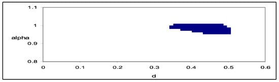
Figure 6.
(αo, do)-values for which Ho (7) cannot be rejected. Nile river data. The region in blue corresponds to the values of α and d for which the null hypothesis cannot be rejected at the 95% level.
The second series examined is monthly temperatures in the Northern Hemisphere over the years 1854–1989, which were obtained from the database of the Climate Research Unit of the University of East Anglia, Norwich, England []. More precisely, this series reports the temperature (degrees C) difference (anomaly) from the monthly average over the period 1950–1979, and its plot ([] p. 30) suggests an upward trend that may reflect global warming during the last 100 years. See also [,,,,,].
It can be seen that in the case of the model without regressors, the null is rejected for all values of αo and do. When including a linear time trend there is a wide range of non-rejection values, which are displayed in Figure 7. These are between 0.32 and 0.57 for do and between 0.8 and 1 for αo. The lowest statistic corresponds to αo = 0.97 and do = 0.40, which implies short memory but with an AR coefficient very close to 1. Ref. [] used a Whittle estimator for d in an ARFIMA(0, d, 0) model with a linear time trend and estimated the value of d to be 0.37 and the trend coefficient to be 0.00032.
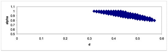
Figure 7.
(αo, do)-values for which Ho (7) cannot be rejected. Northern Hemisphere data. The region in blue corresponds to the values of α and d for which the null hypothesis cannot be rejected at the 95% level.
The third series reports high-precision weight measurements of a 1 kg check standard weight performed at the National Institute of Standards and Technology (NIST, formerly, NBS), Gaithersburg, MD, USA (see [,,,,]). The measurements were taken between 24 June 1963 and 17 October 1975, using the same weight machine. The differences (in micrograms) from 1 kg were recorded. One difficulty with this dataset is that the dates at which measurements were taken are not equidistant. This makes the analysis of short-term correlation problematic. However, the overall long-range dependence structure is likely to be largely unaffected. In the case of this series, when including no regressors, all non-rejection values occur for αo = 1 (i.e., long memory), with values of do ranging between 0.93 and 1.13. However, if an intercept is also included in the model, the region of non-rejection values is wider (see Figure 8) with αo equal to or slightly smaller than 1 and do ranging between 0.02 and 0.23. The lowest statistic occurs at αo = 0.98 and do = 0.11, and setting αo = 1 and do = 0.13. By applying standard semi-parametric long memory methods, ref. [] found in this case estimates of d ranging between 0.02 and 0.28, and when using other, more robust techniques (p. 140), an estimate of about 0.10.
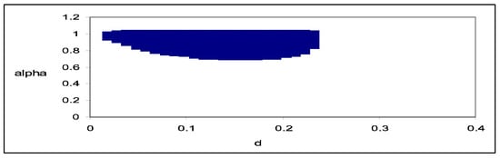
Figure 8.
(αo, do)-values for which Ho (7) cannot be rejected; 1 kg standard weight NIST. The region in blue corresponds to the values of α and d for which the null hypothesis cannot be rejected at the 95% level.
Finally, we analyzed daily data on stock market returns in Venezuela, Argentina, Brazil, Mexico and Colombia, which were obtained from the International Monetary Fund database. The starting date is 4 January 1988 for Argentina and Mexico, 2 January 1990 for Venezuela, 2 January 1992 for Colombia, and 4 July 1994 for Brazil. The end date is 22 January 2002 in all cases. Stock market returns have been examined with long memory and fractional integration techniques in numerous papers, including [,,], among many others.
It can be seen in Table 7 that for Mexico, α is exactly equal to 1, which implies long memory with an order of integration equal to 0.13. Short memory is found in all other cases. In particular, for Colombia, α = 0.87 and d = 0.33; for Argentina, α = 0.57 and d = 0.21; and for Venezuela and Brazil, d = 1.92 but α is then very close to 0 (0.09 for Venezuela and 0.06 for Colombia). We checked the validity of the above models by testing for autocorrelation on the residuals of the selected models. The results achieved using Box–Pierce-type statistics supported the null of no autocorrelation in all cases examined.
Table 7.
Estimates of α and d for each country.
Table 8 reports the impulse response for each series; these are significant in all cases in the first period, up to the third period in Mexico, and up to the fifth in Colombia.
Table 8.
Impulse response functions of the selected models for each country.
6. Conclusions
This paper proposes a general statistical model in the time domain (with a corresponding testing procedure) which is based on the concept of fractional integration and allows the roots of the process to be not only on but also within the unit circle. This is because a fractional root can be any real number, and therefore may or may not lie on the unit circle. As a result, we introduce a model with a high degree of flexibility, incorporating time dependencies that may decay at a lower rate than the exponential ones but faster than with the hyperbolic rates associated, respectively, with the autoregressive and fractional processes. The evidence, based on both Monte Carlo simulations and some empirical applications, shows that the proposed framework performs well in finite samples and accurately captures the stochastic behavior of various series, ranging from climatological to financial ones. Future work could extend the proposed model to allow for cyclical structures, where the singularity or pole in the spectrum occurs at one or more frequencies away from zero.
Author Contributions
Conceptualization, G.M.C. and L.A.G.-A.; Methodology, G.M.C. and L.A.G.-A.; Software, L.A.G.-A.; Formal analysis, L.A.G.-A.; Data curation, L.A.G.-A.; Writing—original draft, L.A.G.-A.; Writing—review & editing, G.M.C. All authors have read and agreed to the published version of the manuscript.
Funding
Luis A. Gil-Alana gratefully acknowledges financial support from the project from ‘Ministerio de Ciencia, Innovación y Universidades’ Agencia Estatal de Investigación’ (AEI) Spain and ‘Fondo Europeo de Desarrollo Regional’ (FEDER), Grant D2023-149516NB-I00 funded by MCIN/AEI/10.13039/501100011033. He also acknowledges support from an internal project of the Universidad Francisco de Vitoria.
Data Availability Statement
The data presented in this study are openly available in National Institute of Standards and Technology (NIST), www.nist.gov.
Acknowledgments
Comments from the Editor and four anonymous reviewers are gratefully acknowledged.
Conflicts of Interest
The authors declare no conflict of interest.
Appendix A. Derivation of the Score Statistic
The negative of the log-likelihood under (1) and Gaussianity of ut is given by
for any admissible α, d and σ2. Then,
so that
where Using the expansion in (11), we obtain that
where
Similarly,
and using (12),
Finally, and this last expression vanishes for It also follows that the expectation in (9) is
where is a (2 × 2) matrix formed by the elements in (13), which can be asymptotically approximated (for ) by in (14). Then, using (9), we deduce .
Appendix B. Proof of Theorem 1
Proof.
Note that the test statistic is based on the Lagrange Multiplier (LM) principle and thus everything is evaluated under the null hypothesis Ho (7), using αo and do in the equations and with the residuals being I(0).
Calling = , , and following conditions (18) and (19) along with Class H of functions for = as defined in Robinson (1994, p. 1433) [], the proof is a straightforward extension of that of Theorem 1 in that paper using Lemmas 1, 2 and 3 and an application of a martingale difference Central Limit Theorem as in []. Specifically, the proof that follows from the fact that are stationary martingale differences. □
References
- Granger, C.W.J. Long memory relationships and the aggregation of dynamic models. J. Econom. 1980, 14, 227–238. [Google Scholar] [CrossRef]
- Hosking, J.R.M. Fractional differencing. Biometrika 1981, 68, 168–176. [Google Scholar] [CrossRef]
- Robinson, P.M. Efficient tests of nonstationary hypotheses. J. Am. Stat. Assoc. 1994, 89, 1420–1437. [Google Scholar] [CrossRef]
- Baillie, R.T. Long memory processes and fractional integration in econometrics. J. Econom. 1996, 73, 5–59. [Google Scholar] [CrossRef]
- Sowell, F. Maximum likelihood estimation of stationary univariate fractionally integrated time series models. J. Econom. 1992, 53, 165–188. [Google Scholar] [CrossRef]
- Granger, C.W.J.; Joyeux, R. An introduction to long memory time series and fractionally differencing. J. Time Ser. Anal. 1980, 1, 15–29. [Google Scholar] [CrossRef]
- Diebold, F.X.; Rudebusch, G.D. Long memory and persistence in aggregate output. J. Monet. Econ. 1989, 24, 189–209. [Google Scholar] [CrossRef]
- Gil-Alana, L.A.; Robinson, P.M. Testing of unit roots and other nonstationary hypotheses in macroeconomic time series. J. Econom. 1997, 80, 241–268. [Google Scholar] [CrossRef]
- Gil-Alana, L.A.; Hualde, J. Fractional Integration and Cointegration: An Overview and an Empirical Application. In Palgrave Handbook of Econometrics; Mills, T.C., Patterson, K., Eds.; Palgrave Macmillan: London, UK, 2009. [Google Scholar] [CrossRef]
- Huade, J.; Nielsen, S. Fractional integration and cointegration. Oxf. Res. Encycl. Econ. Financ. 2023. [Google Scholar] [CrossRef]
- Rao, C.R. Linear Statistical Inference and Its Applications; John Wiley: Hoboken, NJ, USA, 1973. [Google Scholar]
- Toussoun, O. Memoire sur l’historie du Nil. In Memoires a L’Institut D’Eggipte; Institut Français d’Archéologie Orientale: Cairo, Egypt, 1925; Volume 18, pp. 366–404. [Google Scholar]
- Beran, J. Statistics for Long Memory Processes; Clapman and Hall: New York, NY, USA, 1994. [Google Scholar]
- Mudelsee, M. Long memory of rivers from spatial aggregation. Water Resour. Res. 2007, 43. [Google Scholar] [CrossRef]
- Rickert, J. Long Memory and the Nile: Herodotus, Hurst and H. 2014. Available online: https://blog.revolutionanalytics.com/2014/09/intro-to-long-memory-herodotus-hurst-and-h.html (accessed on 12 June 2013).
- Abdelaziz, S.; Ahmed, A.M.M.; Eltahan, A.M.; Elhamid, A.M.I.A. Long-Term Stochastic Modeling of Monthly Streamflow in River Nile. Sustainability 2023, 15, 2170. [Google Scholar] [CrossRef]
- Elgendy, R.; Coulibaly, P.; Hassini, S.; El-Dakhakhni, W.; Elsaie, Y.; Tolera, M.B.; Hatiye, S.D.; Ayana, M. Assessment of monthly to daily streamflow disaggregation methods: A case study of the Nile River Basin. J. Hydrol. Reg. Stud. 2024, 56, 101969. [Google Scholar] [CrossRef]
- Jones, P.D.; Briffa, K.R. Global surface air temperature variations during the twentieth century: Part I Spatial, temporal and seasonal details. Holocene 1992, 2, 165–179.b. [Google Scholar] [CrossRef]
- Mann, M.E.; Bradley, R.S.; Hughes, M.K. Northern hemisphere temperatures during the past millennium: Inferences, uncertainties, and limitations. Geophys. Res. Lett. 1999, 26, 759–762. [Google Scholar] [CrossRef]
- Ljungqvist, F.C.; Krusic, P.; Brattstrom, G.; Sundqvist, H.S. Northern Hemisphere temperature patterns in the last 12 centuries. Clim. Past 2012, 8, 227–249. [Google Scholar] [CrossRef]
- Ogurtsov, M.G. New paleoclimatic evidence of an extraordinary rise in temperature in the Northern Hemisphere in the last 3–4 decades. Geogr. Ann. Ser. A Phys. Geogr. 2022, 104, 288–297. [Google Scholar] [CrossRef]
- Sevgin, F.; Ozturk, A. Variation of temperature increase rate in the Northern Hemisphere according to latitude, longitude and altitude: The Turkey example. Sci. Rep. 2024, 14, 18207. [Google Scholar] [CrossRef] [PubMed]
- Gil-Alana, L.A.; Carmona-Gonzalez, N. Temperature Anomalies in the Northern and Southern Hemispheres: Evidence of Persistence and Trends. Adv. Meteorol. 2024, 2024, 8900065. [Google Scholar] [CrossRef]
- Caporale, G.M.; Gil-Alana, L.A.; Carmona-Gonzalez, N. Some new evidence using fractional integration about trends, breaks and persistence in polar amplification. Sci. Rep. 2025, 15, 8327. [Google Scholar] [CrossRef] [PubMed]
- Pollak, M.; Croarkin, C.; Hagwood, C. Surveillance Schemes with Applications to Mass Calibration; NIST Technology Report 5158; National Institute of Standards and Technology: Gaithersburg, MD, USA, 1993. [Google Scholar]
- Graf, H.P. Long Range Correlation and Estimation of the Self Similarity Parameter. Ph.D. Thesis, ETH Zurich, Zurich, Switzerland, 1983. [Google Scholar]
- Graf, H.P.; Hampel, F.R.; Tacier, J. The problem of unsuspected serial correlation. In Robust and Non-linear Time Series Analysis; France, J., Härdle, W., Martin, R.D., Eds.; Lecture Notes in Statistics; Springer: New York, NY, USA, 1984; Volume 26, pp. 127–145. [Google Scholar]
- Kubarych, Z.J.; Abbott, P.J. The Dissemination of Mass in the United States: Results and Implications of Recent BIPM Calibration of US National Prototype Kilograms. J. Res. Natl. Inst. Stand. Technol. 2014, 119, 1–5. [Google Scholar] [CrossRef]
- Kubarych, Z.J.; Yaniv, S.L. The Kilogram and Measurements of Mass and Force. J. Res. Natl. Inst. Stand. Technol. 2001, 106, 25–46. [Google Scholar] [CrossRef] [PubMed]
- Mishra, A.K.; Mishra, S. Revisiting the Long Memory in Global Stock Market Returns: An Empirical Analysis. Glob. Bus. Rev. 2020, 26, 24–38. [Google Scholar] [CrossRef]
- Caporale, G.M.; Gil-Alana, L.A.; You, K. Stock Market Linkages between the Asean Countries, China and the US: A Fractional Integration/cointegration Approach. Emerg. Mark. Financ. Trade 2022, 58, 1502–1514. [Google Scholar] [CrossRef]
- Bhattacharya, S.; Bhattacharya, M. Long memory in stock returns. A study of emerging markets. Iran. J. Manag. Stud. 2025, 5, 67–88. [Google Scholar]
- Brown, B.M. Martingale Central Limit Theorems. Ann. Math. Stat. 1971, 42, 59–66. [Google Scholar] [CrossRef]
Disclaimer/Publisher’s Note: The statements, opinions and data contained in all publications are solely those of the individual author(s) and contributor(s) and not of MDPI and/or the editor(s). MDPI and/or the editor(s) disclaim responsibility for any injury to people or property resulting from any ideas, methods, instructions or products referred to in the content. |
© 2025 by the authors. Licensee MDPI, Basel, Switzerland. This article is an open access article distributed under the terms and conditions of the Creative Commons Attribution (CC BY) license (https://creativecommons.org/licenses/by/4.0/).