Orthonormal Right-Handed Frames on the Two-Sphere and Solutions to Maxwell’s Equations via de Broglie Waves

Abstract

This paper explores some frame bundles and physical implications of Killing vector fields on the two-sphere ${\mathbb{S}}^2$, culminating in a novel application to Maxwell’s equations in free space. Initially, we investigate the Killing vector fields on ${\mathbb{S}}^2$ (represented by the unit sphere of ${\mathbb{R}}^3$), which generate the isometries of the sphere under the rotation group $SO\left(3\right)$. These fields, realized as functions $K_v:{\mathbb{S}}^2\to {\mathbb{R}}^3$, defined by $K_v\left(q\right)=v\times q$ for a fixed $v\in {\mathbb{R}}^3$ and any $q\in {\mathbb{S}}^2$, generate a three-dimensional Lie algebra isomorphic to $\mathfrak{so}\left(3\right)$. We establish an isomorphism $K:{\mathbb{R}}^3\to \mathcal{K}\left({\mathbb{S}}^2\right)$, mapping vectors $v=au$ (with $u\in {\mathbb{S}}^2$) to scaled Killing vector fields $a{K}_u$, and analyze its relationship with $SO\left(3\right)$ through the exponential map. Subsequently, at a fixed point $e\in {\mathbb{S}}^2$, we construct a smooth orthonormal right-handed tangent frame $f_e:{\mathbb{S}}^2\backslash \{e,-e\}\to T{\left({\mathbb{S}}^2\right)}^2$, defined as $f_e\left(u\right)=({\widehat{K}}_e\left(u\right),u\times {\widehat{K}}_e\left(u\right))$, where ${\widehat{K}}_e$ is the unit vector field of the Killing field $K_e$. We verify its smoothness, orthonormality, and right-handedness. We further prove that any smooth orthonormal right-handed frame on ${\mathbb{S}}^2\backslash \{e,-e\}$ is either $f_e$ or a rotation thereof by a smooth map $\rho :{\mathbb{S}}^2\backslash \{e,-e\}\to SO\left(3\right)$, reflecting the triviality of the frame bundle over the parallelizable domain. The paper then pivots to an innovative application, constructing solutions to Maxwell’s equations in free space by combining spherical symmetries with quantum mechanical de Broglie waves in tempered distribution wave space. The deeper scientific significance lies in bringing together differential geometry (via $SO\left(3\right)$ symmetries), quantum mechanics (de Broglie waves in Schwartz distribution theory), and electromagnetism (Maxwell’s solutions in Schwartz tempered complex fields on Minkowski space-time), in order to offer a unifying perspective on Maxwell’s electromagnetism and Schrödinger’s picture in relativistic quantum mechanics.

1. Introduction: Geometric Symmetries and Maxwell’s Equations on the Two-Sphere

The two-sphere ${\mathbb{S}}^2$, a fundamental object in differential geometry, exhibits rich symmetry properties governed by the rotation group $SO\left(3\right)$, making it a cornerstone for studying geometric structures and their physical applications ([1,2,3]). Killing vector fields, which generate isometries on ${\mathbb{S}}^2$—in the standard form of one-parameter groups of rotations—encapsulate these symmetries and form a Lie algebra isomorphic to $\mathfrak{so}\left(3\right)$, providing a powerful framework for analyzing rotational dynamics. Concurrently, orthonormal tangent frames on ${\mathbb{S}}^2$ offer a means to probe its local geometry, with applications ranging from gauge theories to field theories in physics. In parallel, Maxwell’s equations, the cornerstone of classical electromagnetism, describe electromagnetic wave propagation, with plane wave solutions playing a pivotal role in optics, photonics, and quantum field theory. The integration of geometric symmetries with quantum mechanical concepts, such as de Broglie waves, presents an opportunity to explore novel solutions to these equations, bridging mathematics and physics in innovative ways.

This paper investigates the interplay between the geometric symmetries of ${\mathbb{S}}^2$, which in our paper is realized as the unit sphere of ${\mathbb{R}}^3$, and electromagnetic phenomena, culminating a new method for constructing solutions to Maxwell’s equations in free space. We begin by establishing an isomorphism between ${\mathbb{R}}^3$ and the space of Killing vector fields on ${\mathbb{S}}^2$, mapping vectors to infinitesimal rotations and elucidating their relationship with $SO\left(3\right)$. By fixing a unit vector e in the unit sphere ${\mathbb{S}}^2$, we then construct a smooth orthonormal right-handed tangent frame $f_e$ on the pierced sphere $M_e={\mathbb{S}}^2\backslash \{e,-e\}$. The frame $f_e$ is derived from certain Killing vector fields $K_e$, and we demonstrate that all smooth orthonormal right-handed tangent frames on $M_e$ are rotations (fields of rotations) of this canonical frame $f_e$, leveraging the topological properties of the frame bundle. The core contribution lies in applying these geometric structures to generate electromagnetic fields by combining such a complex-valued frame with de Broglie waves. Specifically, we define a field

$$w_k\left(x\right)=e^{i⟨k,x⟩}(r_k+i{s}_k),$$

where the frame $(r_k,s_k,u_k)$ extends the spherical frame $f_e$ to the dual Minkowski space, satisfying

$$u\times s=-r,$$

where $u_k$ is the unit vector of the spatial part of k, and u is the mapping sending each k to such unit vector $u_k$. This field satisfies Maxwell’s equations for light-like wavevectors, producing circularly polarized plane waves.

Our work brings together differential geometry, quantum mechanics, and Maxwell’s electromagnetism, offering a geometric perspective on electromagnetic wave propagation.

1.1. Preliminary Discussion

The paper aims to provide a new description of electromagnetic phenomena and of basic quantum phenomena in a unifying perspective, adopting:

• The geometric symmetries of the two-dimensional sphere and, in particular, its infinitesimal generators (Killing vector fields),
• The de Broglie basis (momentum basis) of quantum mechanics, in the precise context of Schwartz Distribution Theory and Schwartz Linear Algebra, for complex distributions defined upon the Minkowski (linear) space-time,
• The relativistic Schrödinger equation, massless and massive, in the above-mentioned space of tempered distributions,
• Maxwell’s equations, in their complex form, in the precise context of complex tempered (distribution) three-field space.

These are adopted in order to formulate a new method for constructing solutions to Maxwell’s equations, in free space—both in the massless (light) case and in a generalized massive case (covering spin 0 massive quantum particles)—by linearly embedding vast subfamilies ${\eta }^e$ of the de Broglie basis $\eta$ of quantum mechanics into the complex Maxwell–Schwartz tempered field space ${\mathcal{S}}^{\prime }({\mathbb{M}}_4,{\mathbb{C}}^3)$.

In this sense, and only in this sense, the paper brings together various fields of mathematics and physics in order to give a more unifying perspective on relativistic quantum mechanics (in tempered distribution spaces) and electromagnetism (in tempered field spaces) via spherical symmetries.

More specifically, we realize the two-sphere by the frontier of the unit ball of the spatial part of the dual of Minkowski vector space-time.

For every spatial unit vector $e\in {\mathbb{S}}^2=\partial B(0_3,1)$, we construct a complete continuous-indexed family $w^e$ containing plane-wave solutions (massless and massive fields) of the Maxwell’s complex field equations (and one of its massive generalizations)—in the space of tempered complex three-fields.

We underline that our approach provides a complete scenario of plane-wave solutions, in the sense that each family $w^e$ contains solutions of our generalized Maxwell complex field equations, for the massive $m_0$-case, for each rest mass $m_0\in \mathbb{R}$. In the particular case where $m_0=0$, we are working on the light cone of equation

$$<k,k>=0,$$

with corresponding classic electromagnetic plane-wave solutions $w_k^e$.

Letting the rest mass $m_0$ vary upon the positive real line, we cover the entire time-like dual of Minkowski space by the classic hyperboloid of equation

$$<k,k>=-{\left(m_{0}c\right)}^2/{\hslash }^2.$$

Such vast families $w^e$ (with $e\in {\mathbb{S}}^2$) are constructed by multiplying two complex objects:

• A vast subfamily ${\eta }^e$ of de Broglie waves (from quantum mechanics in tempered distribution spaces) carrying the physical content of the field;
• A purely geometric object $f_e$, chosen among a family of orthonormal smooth frames

  $$f={\left(f_s\right)}_{s\in {\mathbb{S}}^2},$$

  of real dimension 2.

Where $f_e$ is a very specific smooth, orthonormal, bi-dimensional (see later for definition), sphere-tangent (see later), right-handed (see later) frame

$$f_e:{\mathbb{M}}_4^{*}\backslash span(e_0,e)\to {\mathbb{R}}^3\times {\mathbb{R}}^3:f_e=(r_e,s_e)=r_e+ıs_e,$$

of real dimension 2 (complex dimension 1, we insist), defined on the dual of Minkowski space minus a certain plane generated by the unit vector e, associated with $f_e$, and the canonical vector $e_0=(1,0,0,0)$.

Any such frame $f_e$ determines the polarizations (spatial direction) of all the members $w_k^e$ of the associated family $w^e$.

We want to underline some points here:

• In our model, the sphere ${\mathbb{S}}^2$ is identified with (if you prefer, concretely realized by) the unit sphere of the space ${\mathbb{R}}^3$, three-space viewed as the spatial Cartesian factor of the dual of Minkowsky space

  $${\mathbb{M}}_4^{*}=\mathbb{R}\times {\mathbb{R}}^3;$$
• For any point e of ${\mathbb{S}}^2$, we construct a (different) smooth frame $f_e$;
• The phrase “of real dimension 2” means that any value $f_e\left(k\right)$ is an ordered pair of two linearly independent real three-vectors;
• Orthonormal means that all those pairs are orthonormal with respect to the standard inner product of the real three-space;
• Sphere-tangent means that all those pairs $f_e\left(k\right)$ (of orthonormal spatial vectors) are tangent to the (spatial) sphere of the center of the three-origin and passing through $\overrightarrow{k}$ (the spatial part of k, which can, as usual, be viewed as a vector or as a point);
• Right-handed means that the determinant of the triple $(r_e\left(k\right),s_e\left(k\right),\overrightarrow{k})$ is positive, for every k in the domain of $f_e$, where $\overrightarrow{k}$ is the spatial part of k.

We insist that, for every point e of the unit sphere, we associate a frame $f_e$, and a complex field $w^e$; we call e and its opposite the poles of $f_e$ and $w^e$, as well as the poles of the pierced sphere ${\mathbb{S}}^2\backslash \{e,-e\}$; we shall study the properties of such entities; for example, fixed e in the sphere, and we shall study the properties of the frame $f_e$ or of the corresponding $w^e$.

For any $e\in {\mathbb{S}}^2$—the sphere is always seen as a submanifold of ${\mathbb{R}}^3$, or ${\mathbb{R}}^4$—we consider the manifold $M_e$ obtained from the unit sphere by eliminating exactly that e and its opposite. It is a perfectly defined manifold, with differential structure induced canonically by that of ${\mathbb{S}}^2$.

We have infinitely many pierced spheres $M_e$, one for every $e\in {\mathbb{S}}^2$. Clearly, $M_e=M_{-e}$.

All so-defined, pierced spheres are mutually isometric Riemannian manifolds. Any $M_e$ can be isometrically and smoothly transformed onto $M_{{\overrightarrow{e}}_1}$ (pierced sphere obtained from ${\mathbb{S}}^2$ by deleting the canonical vector $(1,0,0)$ and its opposite), applying a convenient rotation of the three-space.

Even in this extreme case, where the pierced spheres $M_e$ are all isometrically diffeomorphic to each other, we shall distinguish among them. We need all the pierced spheres to represent the physical reality of electromagnetic waves (indeed, it suffices to use three pierced spheres, with associated linearly independent Killing vector fields, but this is not relevant in this precise moment: in any case, we should study the generic $M_e$ and its associated differential structures $K_e$, $f_e$, and its associated Schwartz structures ${\eta }^e$, $w^e$).

We define a frame $g=(r,s,u)$ over the dual Minkowski space ${\mathbb{M}}_4^{*}\backslash {\mathsf{\Pi }}_e$, with

$$u_k={\displaystyle \frac{\mathbf{k}}{\left|\mathbf{k}\right|}},$$

extended from $f_e$, satisfying $u\times s=-r$. The complex fields

$$w_k^e\left(x\right)=e^{i⟨k,x⟩}(r_k+i{s}_k),$$

where the waves

$${\eta }_k^e\left(x\right)=e^{i(\mathbf{k}·\mathbf{x}-{\omega }_{k}t)}$$

constitute the de Broglie family ${\eta }^e$, are shown to satisfy Maxwell’s equations for light-like 4-wavevectors k, with

$$\nabla \times w_k^e=\left|\mathbf{k}\right|w_k^e$$

and

$$i{\displaystyle \frac{\partial w_k^e}{\partial t}}=c\left|\mathbf{k}\right|w_k^e.$$

The frame’s orientation aligns with circularly polarized plane wave solutions.

1.2. Possible Applications of Our Model

By leveraging $SO\left(3\right)$ symmetries and quantum phase factors, our work provides a novel framework with potential applications in optics, photonics, and gauge theories.

The direct connection established between the Killing vector fields on ${\mathbb{S}}^2$ and the solutions of Maxwell’s equations has significant application potential in the field of electromagnetic inverse problems. This research not only provides a new perspective for understanding the geometric properties of electromagnetic fields but also opens up new ideas for solving inverse problems. By utilizing the symmetry of the Killing vector fields, researchers can more effectively construct solutions for electromagnetic fields and improve the accuracy of signal inversion in complex systems. Furthermore, the results of this study can provide theoretical support for subsequent research in related fields, facilitating the solution and analysis of inverse problems in applications such as medical imaging and geophysical exploration. Recent advancements in this field are presented in [4,5,6].

1.3. Organization of the Paper

The paper is organized as follows: Section 2 presents the literature review; Section 3 details the Killing vector field isomorphism; Section 4, Section 5, Section 6, Section 7 and Section 8 construct the canonical Killing tangent frames and relative geometric results; Section 9 and Section 10 present the Maxwell applications; Section 11 discusses implications and future directions. In the four appendices, we provide more details about the various concepts used in the paper. In particular, Appendix A presents the needed facts about: geometric symmetries in quantum mechanics; smooth frames on general manifolds; circularly polarized EM-waves; maximally symmetric manifolds; states in QM as tempered distributions. Appendix B presents a long proof about the bundle of orthonormal frames on our pierced spheres. Appendix C presents a brief recap on orientability by Gauss mappings. Appendix D dives into the relationship between our isomorphism K and the Lie group SO(3).

2. Literature Review

The study of Killing vector fields and their geometric implications on manifolds like the two-sphere ${\mathbb{S}}^2$ has a rich history in differential geometry and mathematical physics. Killing vector fields, introduced by Wilhelm Killing in the late 19th century, are vector fields that generate isometries, preserving the metric of a Riemannian manifold [7]. On ${\mathbb{S}}^2$, a maximally symmetric two-dimensional manifold with isometry group $SO\left(3\right)$, Killing vector fields correspond to infinitesimal rotations, forming a three-dimensional Lie algebra isomorphic to $\mathfrak{so}\left(3\right)$ [8]. This isomorphism, mapping vectors in ${\mathbb{R}}^3$ to $\mathcal{K}\left({\mathbb{S}}^2\right)$, is well-documented in texts like Nakahara (2003) and Lee (2018), which detail the relationship between Lie groups and their algebras in geometric contexts [9,10]. Our paper establishes this isomorphism

$$K:{\mathbb{R}}^3\to \mathcal{K}\left({\mathbb{S}}^2\right),$$

where $K_v\left(q\right)=v\times q$, and explores its interplay with $SO\left(3\right)$ via the adjoint action and exponential map, aligning with classical results while emphasizing practical applications.

The construction of orthonormal tangent frames on manifolds is a fundamental topic in differential geometry, with applications in physics and gauge theory. On ${\mathbb{S}}^2$, the frame bundle is non-trivial, but over ${\mathbb{S}}^2\backslash \{e,-e\}$, it becomes trivial due to the domain’s contractibility [11]. Works like Kobayashi and Nomizu (1963) provide a theoretical basis for frame bundles, while our paper specifically constructs a new smooth orthonormal right-handed frame

$$f_e\left(u\right)=({\widehat{K}}_e\left(u\right),u\times {\widehat{K}}_e\left(u\right)),$$

where

$${\widehat{K}}_e\left(u\right)={\displaystyle \frac{e\times u}{|e\times u|}}$$

is the unit vector of the Killing field $K_e\left(u\right)=e\times u$ [12]. We prove that all such frames are obtained from $f_e$ by smooth fields of rotations, leveraging the triviality of the bundle, a result consistent with topological arguments in Milnor and Stasheff (1974) [13]. The right-handedness condition,

$${\widehat{K}}_e\left(u\right)\times (u\times {\widehat{K}}_e\left(u\right))=u,$$

connects to orientation studies in differential geometry [14].

The application of differential geometric structures to electromagnetic theory, particularly Maxwell’s equations, has been explored extensively. Maxwell’s equations in free space describe electromagnetic wave propagation, with plane wave solutions being fundamental [2]. Circularly polarized plane waves, crucial in optics and photonics, are well-studied in texts like Born and Wolf (1999) [15]. The use of electromagnetic complex fields

$$\mathbf{F}=\mathbf{E}+ic\mathbf{B}$$

to simplify Maxwell’s equations aligns with relativistic formulations [1]. Recent works, such as those by Bialynicki-Birula (1996), explore photon wave functions, linking electromagnetic fields to quantum mechanics [16]. However, the literature lacks a direct construction of Maxwell solutions using ${\mathbb{S}}^2$ symmetries and the de Broglie basis of Schwartz linear algebra ([17,18,19,20]).

Our paper introduces a novel application, constructing a fundamental family of solutions w, defined by

$$w_k\left(x\right)=e^{i⟨k,x⟩}(r_k+i{s}_k)$$

for light-like 4-wavevectors k, where the frame $g=(r,s,u)$ extends $f_e$ to the dual Minkowski space ${\mathbb{M}}_4^{*}\backslash \mathsf{\Pi }$, with $u\times s=-r$, or it is a smooth orthonormal right-handed frame obtained by $f_e$ applying a surface of rotations. This approach, inspired by quantum mechanical de Broglie waves [21], unifies differential geometry, quantum mechanics, and electromagnetism. While geometric methods in gauge theory (e.g., Yang–Mills) are discussed in Bleecker (1981), our specific use of Killing vector field-derived frames is unique [22]. Our original frame’s orientation, ensuring $u\times s=-r$, aligns with circular polarization properties [23].

This work fills a gap in the literature by demonstrating how $SO\left(3\right)$ symmetries on ${\mathbb{S}}^2$ can generate physically meaningful electromagnetic solutions, offering a geometric perspective on wave propagation. It extends Schwartz linear algebra by integrating quantum phase factors and smooth orthonormal frames viewed also as complex tempered vector fields. Our approach suggests applications in optics, photonics, and quantum field theory.

Further Bibliography

Paper [24] systematically develops Maxwell’s equations in Schrödinger form, using the curl operator as a Hamiltonian for dispersive media. It provides a strong theoretical foundation somewhat aligning with our formulation in Section 9, but without using Schwartz distribution and S-Linear Algebra and with different aims. The paper [25] reduces Maxwell’s equations to a two-level Schrödinger-type evolution for polarization states, resonating with our use of Killing frames to encode polarization, but again without using Schwartz distribution and S-Linear Algebra and with different intent. Ref. [26] offers a quantum-mechanical derivation of the Schrödinger equation from Maxwellian principles, emphasizing the field–wave duality echoed in our embedding of de Broglie fields into Maxwellian Schwartz space, but, also in this case, it is not completely clear the topological structure in which the author works and, in any case, without using Schwartz distribution. Ref. [27] presents a differential-form and frame-field perspective on Maxwell theory, useful for justifying the frame-theoretic nature of our construction but far from Schwartz theories. Ref. [28] explores the role of Killing fields and frames in identifying photon currents and polarization. Ref. [29] examines the relation between Maxwell potentials and Killing frames in curved space-time.

3. Theoretical Background: Isomorphism Between ${\mathbb{R}}^{\mathbf{3}}$ and the Space $\mathcal{K}\left({\mathbb{S}}^{\mathbf{2}}\right)$ of Killing Vector Fields on ${\mathbb{S}}^{\mathbf{2}}$

Let us formalize the relationship between vectors in ${\mathbb{R}}^3$ and Killing vector fields on the two-sphere ${\mathbb{S}}^2$ by means of the map sending a scaled vector $au$ (where $a\in \mathbb{R}$, $u\in {\mathbb{S}}^2$) to the scaled Killing vector field $a{K}_u$ defined below.

3.1. The Correspondence

The space of Killing vector fields on ${\mathbb{S}}^2$, denoted $\mathcal{K}\left({\mathbb{S}}^2\right)$, is a three-dimensional vector space, isomorphic to the Lie algebra $\mathfrak{so}\left(3\right)$, because the isometry group of ${\mathbb{S}}^2$ is $SO\left(3\right)$. For a unit vector $u\in {\mathbb{S}}^2\subset {\mathbb{R}}^3$ (i.e., $\left|u\right|=1$), the Killing vector field is the vector-valued mapping

$$K_u:{\mathbb{S}}^2\to {\mathbb{R}}^3:k\mapsto K_u\left(q\right)=u\times q,$$

for $q\in {\mathbb{S}}^2$. This vector field $K_u$ generates rotations around the axis u, in the sense that it is the infinitesimal generator of the one-parameter group $R_u:\mathbb{R}\to SO\left(3\right)$ sending each $\theta$ to the rotation $R_u\left(\theta \right)$ (see Figure 1).

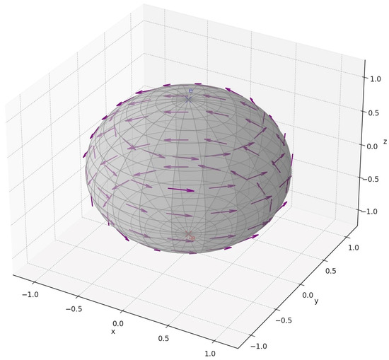
Figure 1. Killing vector field $K_u\left(q\right)=u\times q$ on the sphere.

Now, consider any vector $v\in {\mathbb{R}}^3$, which we can write as:

$$v=au,$$

where $a=\left|v\right|\in {\mathbb{R}}_{\ge 0}$ is the magnitude, and $u=v/\left|v\right|\in {\mathbb{S}}^2$ is a unit vector (if $v\ne 0$). If $v=0$, we will handle that separately. Define the Killing vector field associated with v by

$$K_v\left(q\right)=v\times q.$$

If $v=au$, then

$$K_v\left(q\right)=\left(au\right)\times q=a(u\times q)=a{K}_u\left(q\right).$$

Thus, the Killing vector field $K_v$ is the scaled Killing vector field $a{K}_u$. This suggests a linear map K from ${\mathbb{R}}^3$ to $\mathcal{K}\left({\mathbb{S}}^2\right)$

$${\mathbb{R}}^3\to \mathcal{K}\left({\mathbb{S}}^2\right),v\mapsto K_v,$$

where

$$K_v\left(q\right)=v\times q.$$

3.2. Properties of the Map K

Let us examine this map K.

• Linearity. The map K is linear. For vectors $v_1,v_2\in {\mathbb{R}}^3$ and scalars $c_1,c_2\in \mathbb{R}$:

  $$K_{c_1{v}_1+c_2{v}_2}\left(q\right)=(c_1{v}_1+c_2{v}_2)\times q=c_1(v_1\times q)+c_2(v_2\times q)=c_1{K}_{v_1}\left(q\right)+c_2{K}_{v_2}\left(q\right).$$
• Action on Scaled Vectors. If $v=au$ with $u\in {\mathbb{S}}^2$, then

  $$K_v=a{K}_u.$$
• Zero Vector. If $v=0$, then

  $$K_0\left(q\right)=0\times q=0,$$

  which is the zero vector field, a valid element of $\mathcal{K}\left({\mathbb{S}}^2\right)$.
• Surjectivity. To check if every Killing vector field on ${\mathbb{S}}^2$ is of the form $K_v$, consider a general Killing vector field. We know $\mathcal{K}\left({\mathbb{S}}^2\right)$ is spanned by the basis $(K_1,K_2,K_3)$, where

  $$K_1\left(q\right)=e_1\times q,K_2\left(q\right)=e_2\times q,K_3\left(q\right)=e_3\times q,$$

  and $e_1=(1,0,0)$, $e_2=(0,1,0)$, $e_3=(0,0,1)$. A general Killing vector field is a linear combination

  $$V=a{K}_1+b{K}_2+c{K}_3.$$
  Let us compute the value of V at every point:

  $$V\left(q\right)=a(e_1\times q)+b(e_2\times q)+c(e_3\times q)=(a{e}_1+b{e}_2+c{e}_3)\times q=v\times q,$$

  where $v=(a,b,c)\in {\mathbb{R}}^3$. Thus

  $$V=K_v.$$
  This shows the map $v\mapsto K_v$ is surjective: every Killing vector field on ${\mathbb{S}}^2$ is of the form $K_v$ for some $v\in {\mathbb{R}}^3$.
• Injectivity. Is the map K injective? Suppose $K_{v_1}=K_{v_2}$, then

  $$v_1\times q=v_2\times q,$$

  for all $q\in {\mathbb{S}}^2$. This implies

  $$(v_1-v_2)\times q=0.$$
  Since q represents all vectors on ${\mathbb{S}}^2$, choose q perpendicular to $v_1-v_2$ (if $v_1-v_2\ne 0$, such q exists on ${\mathbb{S}}^2$). The cross product is zero only if $v_1-v_2=0$, because $v_1-v_2$ cannot be parallel to all $q\in {\mathbb{S}}^2$. Thus, $v_1=v_2$, and the map is injective.
• Isomorphism. Since ${\mathbb{R}}^3$ and $\mathcal{K}\left({\mathbb{S}}^2\right)$ are both three-dimensional vector spaces, and the map $v\mapsto K_v$ is linear, surjective, and injective, it is an isomorphism

  $${\mathbb{R}}^3\cong \mathcal{K}\left({\mathbb{S}}^2\right).$$

3.3. Interpretation

We have found a natural correspondence from ${\mathbb{R}}^3$ to $\mathcal{K}\left({\mathbb{S}}^2\right)$, where a vector $v=au$ (with $a\in \mathbb{R}$, $u\in {\mathbb{S}}^2$) maps to the Killing vector field

$$K_v=a{K}_u.$$

This correspondence is not only intuitive but also a vector space isomorphism. Each vector $v\in {\mathbb{R}}^3$ specifies a Killing vector field $K_v$.

• The direction of v (i.e., $u=v/\left|v\right|$) determines the axis of rotation of the associated one-parameter group of rotations $R_u$.
• The magnitude of v (i.e., $a=\left|v\right|$) scales the “strength” of the Killing vector field, affecting the angular speed of the rotation it generates.

For example:

• If $v=(1,0,0)$, then $K_v=K_1$, which generates the rotation group around the first axis.
• If $v=(2,0,0)=2e_1$, then $K_v=2K_1$, a “faster” rotation group around the same axis in the sense that the one-parameter group

  $$\theta \mapsto e^{\theta \left(2A_1\right)}=e^{\left(2\theta \right)A_1}$$

  rotates twice as fast. Here, the matrix $A_1$ is the matrix associated with the linear application $L_1=e_1\times$.
• If $v=0$, then $K_0=0$, the trivial Killing vector field.

We observe that, in general, the killing vector field $K_v$ is the restriction of the linear endomorphism of ${\mathbb{R}}^3$

$$L_v=v\times .$$

3.4. Geometric Insight

The isomorphism ${\mathbb{R}}^3\cong \mathcal{K}\left({\mathbb{S}}^2\right)$ reflects the fact that the Lie algebra $\mathfrak{so}\left(3\right)$ is isomorphic to ${\mathbb{R}}^3$ with the cross product as the Lie bracket. The Killing vector fields are the manifestations of $\mathfrak{so}\left(3\right)$ on ${\mathbb{S}}^2$, and the map $K:v\mapsto v\times$ translates vectors in ${\mathbb{R}}^3$ to these generators of rotations.

Our observation about scaled vectors $au\mapsto a{K}_u$ highlights that the space $\mathcal{K}\left({\mathbb{S}}^2\right)$ includes all possible rotation axes (parametrized by $u\in {\mathbb{S}}^2$) and all possible scalings (parametrized by $a\in \mathbb{R}$), covering the entire three-dimensional space of Killing vector fields.

3.5. Final Remark

We have found a correspondence from ${\mathbb{R}}^3$ to $\mathcal{K}\left({\mathbb{S}}^2\right)$, where a vector $v=au$ (with $a\in \mathbb{R}$, $u\in {\mathbb{S}}^2$) maps to the Killing vector field

$$K_v=a{K}_u,$$

and this map, defined by $K_v\left(q\right)=v\times q$, is an isomorphism between ${\mathbb{R}}^3$ and $\mathcal{K}\left({\mathbb{S}}^2\right)$. Every Killing vector field on ${\mathbb{S}}^2$, including the zero vector field, is uniquely represented by some $v\in {\mathbb{R}}^3$, with scaled vectors $au$ producing scaled Killing vector fields $a{K}_u$, and the Lie bracket structure on the space of Killing vector fields is defined by

$$[K_v,K_w]=K_{v\times w}.$$

4. Results I: Smooth Orthonormal Tangent Frame ${\mathit{f}}_{\mathit{e}}$ on the Two-Sphere

We desire to explore, now, an original aspect of the Killing vector fields $K_e$ on the sphere: their capability to determine a canonical smooth orthonormal frame $f_e$ on the two-sphere minus the “polar” couple $\{e,-e\}$.

At this purpose, we shall state and prove the following original theorem.

Theorem 1. 

Consider a unit vector e of the space ${\mathbb{R}}^3$, that is, an element of ${\mathbb{S}}^2$. Now consider the tangent frame

$$f_e:{\mathbb{S}}^2\backslash \{e,-e\}\to T\left({\mathbb{S}}^2\right)\times T\left({\mathbb{S}}^2\right),$$

defined—on the 2-sphere minus the two poles e and $-e$, and taking values in the Cartesian square of the tangent bundle of ${\mathbb{S}}^2$—by the relation

$$f_e\left(u\right)=({\widehat{K}}_e\left(u\right),u\times {\widehat{K}}_e\left(u\right)),$$

where ${\widehat{K}}_e\left(u\right)$ is the unit vector of $K_e\left(u\right)$.

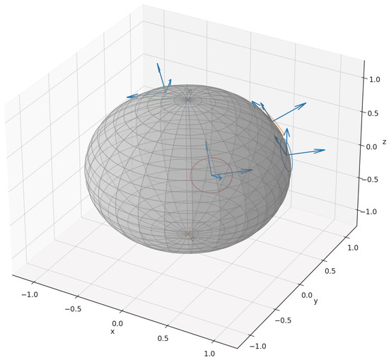
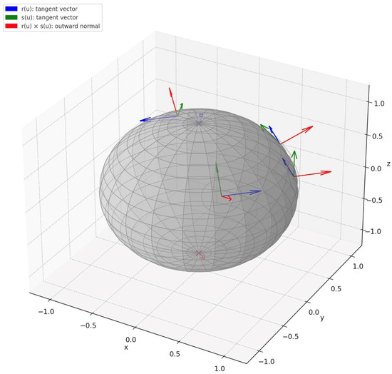
Then, the mapping $f_e$ is a smooth orthonormal tangent frame on ${\mathbb{S}}^2$ minus the poles e and $-e$ (see Figure 2 and Figure 3).

Figure 2. Pierced sphere $M_e={\mathbb{S}}^2\backslash \{e,-e\}$ with local frames and tangent planes.

Figure 3. Multiple local frames on the pierced sphere $M_e={\mathbb{S}}^2\backslash \{e,-e\}$.

4.1. Proof of Theorem 1

Proof of Theorem 1. 

Let us dive into the problem of determining whether the tangent frame

$$f_e:{\mathbb{S}}^2\backslash \{e,-e\}\to T{\left({\mathbb{S}}^2\right)}^2,$$

defined by $f_e\left(u\right)=({\widehat{K}}_e\left(u\right),u\times {\widehat{K}}_e\left(u\right))$, is a smooth orthonormal tangent frame on the two-sphere ${\mathbb{S}}^2$ minus the poles e and $-e$. Here, $e\in {\mathbb{S}}^2\subset {\mathbb{R}}^3$ is a unit vector, $K_e\left(u\right)=e\times u$, and ${\widehat{K}}_e\left(u\right)$ is the unit vector in the direction of $K_e\left(u\right)$. We will prove the theorem in more steps.

Proof Overview. The proof is indeed very simple if we consider the basic properties of the cross product: the two members of our frame are unitary by definition. The first one is a unit vector and the second one is the product of two orthogonal unit vectors. They are orthogonal because the cross product of two vectors is orthogonal to both vectors. The two vectors are both tangent to the sphere because they are both orthogonal to u. The frame is smooth because both components are smooth.

Setup and Definitions.

• The Two-Sphere. ${\mathbb{S}}^2=\{u\in {\mathbb{R}}^3\mid \left|u\right|=1\}$ is the unit sphere in ${\mathbb{R}}^3$, a two-dimensional smooth manifold.
• Unit Vector e. $e\in {\mathbb{S}}^2$, so $\left|e\right|=1$.
• Killing Vector Field. For $e\in {\mathbb{S}}^2$, the associated Killing vector field is defined by

  $$K_e\left(u\right)=e\times u,$$

  where $u\in {\mathbb{S}}^2$. Any vector $K_e\left(u\right)$ is a tangent vector to ${\mathbb{S}}^2$ at u, since

  $$K_e\left(u\right)·u=(e\times u)·u=0,$$

  by properties of the cross product.
• Unit Vector ${\widehat{K}}_e\left(u\right)$. Assuming $K_e\left(u\right)\ne 0$, we define

  $${\widehat{K}}_e\left(u\right)={\displaystyle \frac{K_e\left(u\right)}{|K_e\left(u\right)|}},$$

  where

  $$|K_e\left(u\right)|=|e\times u|=|e\left|\right|u|sin\theta =sin\theta ,$$

  and $\theta$ is the angle between e and u. Since $\left|e\right|=\left|u\right|=1$, we have

  $$|e\times u|=\sqrt{1-{(e·u)}^2},$$

  because

  $$e·u=cos\theta ,sin\theta =\sqrt{1-{cos}^2\theta }.$$

  Thus

  $${\widehat{K}}_e\left(u\right)={\displaystyle \frac{e\times u}{\sqrt{1-{(e·u)}^2}}}.$$
• Tangent Frame. The tangent frame is defined by

  $$f_e:{\mathbb{S}}^2\backslash \{e,-e\}\to T{\left({\mathbb{S}}^2\right)}^2,f_e\left(u\right)=({\widehat{K}}_e\left(u\right),u\times {\widehat{K}}_e\left(u\right)),$$

  where $T{\left({\mathbb{S}}^2\right)}^2=T\left({\mathbb{S}}^2\right)\times T\left({\mathbb{S}}^2\right)$ is the Cartesian product of the tangent bundle with itself, i.e., $f_e\left(u\right)$ assigns a pair of tangent vectors in $T_u{\mathbb{S}}^2$.
• Domain of $f_e$. The domain is ${\mathbb{S}}^2\backslash \{e,-e\}$, because

  $$K_e\left(u\right)=e\times u=0$$

  when $u=\pm e$ (since $e\times e=0$, $e\times (-e)=0$). At these points, ${\widehat{K}}_e\left(u\right)$ is undefined, justifying their exclusion.
• Goal. Determine if $f_e$ is a smooth orthonormal tangent frame, meaning:

  –

  Smooth. $f_e$ is a smooth map, i.e., the vector fields ${\widehat{K}}_e$ and $u\times {\widehat{K}}_e$ are smooth on ${\mathbb{S}}^2\backslash \{e,-e\}$.

  –

  Orthonormal. At each u, the vectors ${\widehat{K}}_e\left(u\right)$ and $u\times {\widehat{K}}_e\left(u\right)$ are:

  ∗

  Tangent to ${\mathbb{S}}^2$ at u.

  ∗

  Orthonormal with respect to the induced metric on ${\mathbb{S}}^2$.

  ∗

  Form a basis for $T_u{\mathbb{S}}^2$.

Step 1: Tangency. First, confirm that both ${\widehat{K}}_e\left(u\right)$ and $u\times {\widehat{K}}_e\left(u\right)$ are tangent to ${\mathbb{S}}^2$ at u.

• ${\widehat{K}}_e\left(u\right)$:

  $${\widehat{K}}_e\left(u\right)={\displaystyle \frac{e\times u}{|e\times u|}}.$$

  Since $K_e\left(u\right)=e\times u$ is tangent (as $(e\times u)·u=0$), and ${\widehat{K}}_e\left(u\right)$ is a scalar multiple of $K_e\left(u\right)$, it is also tangent:

  $${\widehat{K}}_e\left(u\right)·u={\displaystyle \frac{(e\times u)·u}{|e\times u|}}=0.$$
• $u\times {\widehat{K}}_e\left(u\right)$:

  $$u\times {\widehat{K}}_e\left(u\right)=u\times {\displaystyle \frac{e\times u}{|e\times u|}}.$$

  Check tangency:

  $$(u\times {\widehat{K}}_e\left(u\right))·u=\left(u\times {\displaystyle \frac{e\times u}{|e\times u|}}\right)·u=0,$$

  since the cross product $a\times b$ is perpendicular to both a and b. Thus, both vectors lie in $T_u{\mathbb{S}}^2$.

Step 2: Orthonormality. To be an orthonormal frame, the vectors ${\widehat{K}}_e\left(u\right)$ and $u\times {\widehat{K}}_e\left(u\right)$ must be:

• Unit vectors (norm 1 with respect to the metric).
• Orthogonal to each other.
• Linearly independent (to span $T_u{\mathbb{S}}^2$).

The metric on ${\mathbb{S}}^2$ is the induced Euclidean metric from ${\mathbb{R}}^3$, so the inner product of tangent vectors $v,w\in T_u{\mathbb{S}}^2$ is the dot product $v·w$.

• Norm of ${\widehat{K}}_e\left(u\right)$. Since

  $${\widehat{K}}_e\left(u\right)={\displaystyle \frac{e\times u}{|e\times u|}},$$

  then we have

  $$|{\widehat{K}}_e{\left(u\right)|}^2={\displaystyle \frac{{|e\times u|}^2}{{|e\times u|}^2}}=1.$$

  Therefore, ${\widehat{K}}_e\left(u\right)$ is a unit vector.
• Norm of $u\times {\widehat{K}}_e\left(u\right)$. We have

  $$u\times {\widehat{K}}_e\left(u\right)=u\times {\displaystyle \frac{e\times u}{|e\times u|}}.$$

  Let us compute the norm

  $$|u\times {\widehat{K}}_e\left(u\right)|=\left|u\times {\displaystyle \frac{e\times u}{|e\times u|}}\right|={\displaystyle \frac{|u\times (e\times u\left)\right|}{|e\times u|}}.$$

  Using the vector triple product identity

  $$e\times u=-(u\times e),$$

  $$u\times (e\times u)=u\times (u\times e)=(u·e)u-(u·u)e=(u·e)u-e,$$

  since $u·u=1$. Compute the magnitude

  $$|u\times (e\times u\left)\right|=\left|\right(u·e)u-e|.$$

  $${|(u·e)u-e|}^2=((u·e)u-e)·((u·e)u-e)={(u·e)}^{2}u·u-2(u·e)(u·e)+e·e.$$

  Since $u·u=1$, $e·e=1$, we have

  $${|(u·e)u-e|}^2={(u·e)}^2·1-2{(u·e)}^2+1=1-{(u·e)}^2.$$

  Thus

  $$|u\times (e\times u)|=\sqrt{1-{(u·e)}^2}=|e\times u|,$$

  since $|e\times u|=\sqrt{1-{(e·u)}^2}$. So

  $$|u\times {\widehat{K}}_e\left(u\right)|={\displaystyle \frac{|u\times (e\times u\left)\right|}{|e\times u|}}={\displaystyle \frac{|e\times u|}{|e\times u|}}=1.$$

  Thus, $u\times {\widehat{K}}_e\left(u\right)$ is also a unit vector.
• Orthogonality. Let us check the dot product. We have

  $${\widehat{K}}_e\left(u\right)·(u\times {\widehat{K}}_e\left(u\right))={\displaystyle \frac{e\times u}{|e\times u|}}·\left(u\times {\displaystyle \frac{e\times u}{|e\times u|}}\right).$$

  Using the scalar triple product $a·(b\times c)$, we obtain

  $$(e\times u)·(u\times (e\times u\left)\right)=(e\times u)·\left(\right(u·e)u-e)=$$

  $$=(e\times u)·(u·e)u-(e\times u)·e=0-0=0,$$

  since $(e\times u)·u=0$ and $(e\times u)·e=0$. Thus

  $${\widehat{K}}_e\left(u\right)·(u\times {\widehat{K}}_e\left(u\right))={\displaystyle \frac{0}{{|e\times u|}^2}}=0.$$

  The vectors are orthogonal.
• Linear Independence. Since $T_u{\mathbb{S}}^2$ is two-dimensional, two orthonormal vectors form a basis. Alternatively, note that ${\widehat{K}}_e\left(u\right)$ is perpendicular to u, and $u\times {\widehat{K}}_e\left(u\right)$ is perpendicular to both u and ${\widehat{K}}_e\left(u\right)$. Since ${\widehat{K}}_e\left(u\right)\ne 0$ on ${\mathbb{S}}^2\backslash \{e,-e\}$, they are linearly independent.

Thus, $({\widehat{K}}_e\left(u\right),u\times {\widehat{K}}_e\left(u\right))$ is an orthonormal basis of $T_u{\mathbb{S}}^2$.

Step 3: Smoothness. To be a smooth tangent frame, the map

$$f_e:{\mathbb{S}}^2\backslash \{e,-e\}\to T{\left({\mathbb{S}}^2\right)}^2,$$

$u\mapsto ({\widehat{K}}_e\left(u\right),u\times {\widehat{K}}_e\left(u\right))$, must be smooth. Since $T{\left({\mathbb{S}}^2\right)}^2$ is a bundle over ${\mathbb{S}}^2$, we need ${\widehat{K}}_e\left(u\right)$ and $u\times {\widehat{K}}_e\left(u\right)$ to be smooth vector fields on ${\mathbb{S}}^2\backslash \{e,-e\}$.

• Smoothness of ${\widehat{K}}_e\left(u\right)$. We have

  $${\widehat{K}}_e\left(u\right)={\displaystyle \frac{e\times u}{\sqrt{1-{(e·u)}^2}}}.$$

  Numerator. The application $u\mapsto e\times u$ is smooth, as the cross product is a linear map in u, and $u\mapsto u$ is smooth on ${\mathbb{S}}^2$.
  Denominator. The map

  $$u\mapsto |e\times u|=\sqrt{1-{(e·u)}^2}$$

  is smooth. Indeed, the function $u\mapsto u·e$ is smooth (linear in u), and $u\mapsto 1-{(u·e)}^2$ is smooth. We need only

  $$\sqrt{1-{(u·e)}^2}\ne 0,$$

  which holds on ${\mathbb{S}}^2\backslash \{e,-e\}$, since

  $$1-{(u·e)}^2=0\Rightarrow {(u·e)}^2=1\Rightarrow u·e=\pm 1\Rightarrow u=\pm e.$$

  The square root function is smooth on $(0,\infty )$, and $1-{(u·e)}^2>0$ on the domain. Thus, the denominator is smooth.
  Quotient. The quotient of smooth functions, with a non-zero denominator, is smooth. Hence, ${\widehat{K}}_e$ is smooth.

• Smoothness of $u\times {\widehat{K}}_e\left(u\right)$. Concluding the mapping

  $$u\mapsto u\times {\widehat{K}}_e\left(u\right)=u\times {\displaystyle \frac{e\times u}{|e\times u|}}$$

  is smooth since ${\widehat{K}}_e$ is smooth, and the cross product is a smooth (bilinear) operation; therefore, the mapping $u\mapsto u\times {\widehat{K}}_e\left(u\right)$ is smooth.

□

4.2. Conclusions and Canonical Orthonormal Killing Frame

The tangent frame $f_e:f_e\left(u\right)=({\widehat{K}}_e\left(u\right),u\times {\widehat{K}}_e\left(u\right))$ is:

• Tangent. Both vectors’ field components are in $T{\mathbb{S}}^2$.
• Orthonormal. Both vectors’ field components are unit vector fields and mutually orthogonal.
• Smooth. Both vector field components ${\widehat{K}}_e$ and $u\mapsto u\times {\widehat{K}}_e\left(u\right)$ are smooth on ${\mathbb{S}}^2\backslash \{e,-e\}$.

Thus, $f_e$ is a smooth orthonormal tangent frame on ${\mathbb{S}}^2\backslash \{e,-e\}$.

Definition 1. 

We shall call $f_e$ “orthonormal frame induced by $K_e$” or “Killing frame of poles e and $-e$”.

5. Results II: The Tangent Frame ${\mathit{f}}_{\mathit{e}}$ as a Smooth Right-Handed Orthonormal Frame

In this section, we state and prove a second important original point: the Killing frame $f_e=(r_e,s_e)$ is not only smooth and orthonormal but also right-handed, in the sense that the triple $(r_e\left(u\right),s_e\left(u\right),u)$ is right-handed (with positive determinant), for every u in the sphere minus the poles of the frame $f_e$. In other terms, the cross product of $r_e$ times $s_e$ is the identity function on the sphere minus the poles of $f_e$.

Theorem 2. 

The cross product of the first vector field of the Killing frame $f_e$ times the second vector field of $f_e$ gives the identity mapping on ${\mathbb{S}}^2$ (minus the poles of $f_e$).

5.1. Proof of Theorem 2

Proof of Theorem 2. 

Let us investigate whether the cross product of the first vector field of the tangent frame $f_e:{\mathbb{S}}^2\backslash \{e,-e\}\to T{\left({\mathbb{S}}^2\right)}^2$, defined by $f_e\left(u\right)=({\widehat{K}}_e\left(u\right),u\times {\widehat{K}}_e\left(u\right))$, where the second vector field yields the identity mapping on ${\mathbb{S}}^2\backslash \{e,-e\}$. That is, we need to compute:

$${\widehat{K}}_e\left(u\right)\times (u\times {\widehat{K}}_e\left(u\right)),$$

and check if it equals u, the position vector on ${\mathbb{S}}^2$, for all $u\in {\mathbb{S}}^2\backslash \{e,-e\}$. Here, $e\in {\mathbb{S}}^2\subset {\mathbb{R}}^3$ is a unit vector, $K_e\left(u\right)=e\times u$, and

$${\widehat{K}}_e\left(u\right)={\displaystyle \frac{e\times u}{|e\times u|}}.$$

Proof Overview. The proof is a straightforward exercise: it is an obvious application of the vector triple product identity.

Setup and Definitions.

• Two-Sphere. ${\mathbb{S}}^2=\{u\in {\mathbb{R}}^3\mid \left|u\right|=1\}$.
• Unit Vector e. $e\in {\mathbb{S}}^2$, so $\left|e\right|=1$.
• Killing Vector Field. $K_e\left(u\right)=e\times u$, tangent to ${\mathbb{S}}^2$ at u.
• Unit Vector Field.

  $${\widehat{K}}_e\left(u\right)={\displaystyle \frac{e\times u}{|e\times u|}},|e\times u|=\sqrt{1-{(e·u)}^2},$$

  defined on ${\mathbb{S}}^2\backslash \{e,-e\}$, where $e·u=\pm 1$ (i.e., $u=\pm e$) makes $e\times u=0$.
• Second Vector Field.

  $$u\times {\widehat{K}}_e\left(u\right)=u\times {\displaystyle \frac{e\times u}{|e\times u|}}.$$
• Tangent Frame. $f_e\left(u\right)=({\widehat{K}}_e\left(u\right),u\times {\widehat{K}}_e\left(u\right))$, which we have shown is smooth and orthonormal on ${\mathbb{S}}^2\backslash \{e,-e\}$.
• Goal. Compute

  $${\widehat{K}}_e\left(u\right)\times (u\times {\widehat{K}}_e\left(u\right)),$$

  and check if it equals u.

Verification of the Right-Handedness. Let us compute the cross product using vector identities.

$${\widehat{K}}_e\left(u\right)={\displaystyle \frac{e\times u}{|e\times u|}},u\times {\widehat{K}}_e\left(u\right)=u\times {\displaystyle \frac{e\times u}{|e\times u|}}.$$

Define:

$$k=e\times u,\left|k\right|=|e\times u|=\sqrt{1-{(e·u)}^2},$$

$${\widehat{K}}_e\left(u\right)={\displaystyle \frac{k}{\left|k\right|}},u\times {\widehat{K}}_e\left(u\right)=u\times {\displaystyle \frac{k}{\left|k\right|}}.$$

We need:

$${\widehat{K}}_e\left(u\right)\times (u\times {\widehat{K}}_e\left(u\right))={\displaystyle \frac{k}{\left|k\right|}}\times \left(u\times {\displaystyle \frac{k}{\left|k\right|}}\right).$$

Compute the inner cross product:

$$u\times {\displaystyle \frac{k}{\left|k\right|}}={\displaystyle \frac{u\times k}{\left|k\right|}}.$$

Now:

$$k=e\times u,$$

$$u\times k=u\times (e\times u).$$

Use the vector triple product identity:

$$a\times (b\times c)=(a·c)b-(a·b)c,$$

$$u\times (e\times u)=(u·u)e-(u·e)u=e-(u·e)u,$$

since $u·u=1$. Therefore,

$$u\times k=e-(u·e)u,$$

$$u\times {\widehat{K}}_e\left(u\right)={\displaystyle \frac{u\times k}{\left|k\right|}}={\displaystyle \frac{e-(u·e)u}{\left|k\right|}}.$$

Now compute:

$${\widehat{K}}_e\left(u\right)\times (u\times {\widehat{K}}_e\left(u\right))={\displaystyle \frac{k}{\left|k\right|}}\times {\displaystyle \frac{e-(u·e)u}{\left|k\right|}}=$$

$$={\displaystyle \frac{1}{{\left|k\right|}^2}}k\times (e-(u·e)u)=$$

$$={\displaystyle \frac{1}{{\left|k\right|}^2}}[k\times e-(u·e)(k\times u)].$$

• First term:

  $$k=e\times u,$$

  $$k\times e=(e\times u)\times e=(e·e)u-(e·u)e=u-(e·u)e,$$

  since $e·e=1$.

• Second term:

  $$k\times u=(e\times u)\times u=(e·u)u-(u·u)e=(e·u)u-e.$$

  Therefore,

  $$k\times (e-(u·e\left)u\right)=[u-(e·u\left)e\right]-(u·e)\left[\right(e·u)u-e]=$$

  $$=u-(e·u)e-{(u·e)}^{2}u+(u·e)e=$$

  $$=u-{(u·e)}^{2}u+(u·e)e-(e·u)e=$$

  $$=u[1-{(u·e)}^2].$$

  Thus,

  $${\widehat{K}}_e\left(u\right)\times (u\times {\widehat{K}}_e\left(u\right))={\displaystyle \frac{1}{{\left|k\right|}^2}}u[1-{(u·e)}^2].$$

  Since,

  $${\left|k\right|}^2={|e\times u|}^2=1-{(u·e)}^2,$$

  $${\widehat{K}}_e\left(u\right)\times (u\times {\widehat{K}}_e\left(u\right))={\displaystyle \frac{1}{1-{(u·e)}^2}}u[1-{(u·e)}^2]=u.$$

This suggests the cross product yields u, the identity mapping on ${\mathbb{S}}^2\backslash \{e,-e\}$. □

5.2. Geometric Interpretation

The result

$${\widehat{K}}_e\left(u\right)\times (u\times {\widehat{K}}_e\left(u\right))=u$$

means the cross product of the first and second vector fields of the frame $f_e$ yields the position mapping $U_e$, which is nothing but the identity mapping

$$U_e:u\mapsto u$$

on ${\mathbb{S}}^2\backslash \{e,-e\}$. Geometrically, since

$$f_e\left(u\right)=({\widehat{K}}_e\left(u\right),u\times {\widehat{K}}_e\left(u\right))$$

is an orthonormal basis for the tangent space $T_u{\mathbb{S}}^2$, and since u is normal to $T_u{\mathbb{S}}^2$, then the cross product of the basis vectors produces a vector in the normal direction, scaled exactly to u.

5.3. Conclusions

The cross product of the first vector field ${\widehat{K}}_e$ and the second vector field

$$U_e\times {\widehat{K}}_e$$

of the tangent frame $f_e$ gives the identity mapping $U_e$ on ${\mathbb{S}}^2\backslash \{e,-e\}$:

$${\widehat{K}}_e\left(u\right)\times (u\times {\widehat{K}}_e\left(u\right))=u,$$

for every u belonging to ${\mathbb{S}}^2\backslash \{e,-e\}$. We call this last property right-handedness of the frame $f_e$. That is equivalent to state that the triple $(f_e,U_e)=(r_e,s_e,U_e)$ is a right-handed orthonormal frame of ${\mathbb{R}}^3$, defined on ${\mathbb{S}}^2\backslash \{e,-e\}$, where $U_e$ is the identity function of ${\mathbb{S}}^2\backslash \{e,-e\}$.

6. Results III: Orthonormal Right-Handed Frames

In this section, we state and prove the main geometric theorem of the paper, which is perhaps the most intricate to grasp and prove here. We show essentially that all smooth orthonormal right-handed frames on the two sphere, minus two opposite poles, is induced by a Killing frame.

This is also interesting for the original physics application, which sees the transformation of the de Broglie basis into a standard basis of plane waves generating the solution space of the free Maxwell’s equations; this is because it proves that any “orthodox” electromagnetic Maxwellian field is a Schwartz superposition of a basis determined solely by the continuous symmetries of the two sphere (i.e., $SO\left(3\right)$, by means of its Lie algebra) and by the celebrated de Broglie basis of quantum mechanics.

Theorem 3. 

Every smooth orthonormal right-handed frame on ${\mathbb{S}}^2$, minus a prechosen e and its opposite $-e$, should be necessarily $f_e$ or any of its rotation by a smooth rotation field

$$\rho :{\mathbb{S}}^2\backslash \{e,-e\}\to SO\left(3\right).$$

This theorem dives deep into the geometry of tangent frames on the two-sphere ${\mathbb{S}}^2$.

Proof of Theorem 3

Proof of Theorem 3. 

We have defined the tangent frame

$$f_e:{\mathbb{S}}^2\backslash \{e,-e\}\to T{\left({\mathbb{S}}^2\right)}^2,$$

given by

$$f_e\left(u\right)=({\widehat{K}}_e\left(u\right),u\times {\widehat{K}}_e\left(u\right)),$$

where

$${\widehat{K}}_e\left(u\right)={\displaystyle \frac{e\times u}{|e\times u|}},$$

and established its “right-handedness” property:

$${\widehat{K}}_e\left(u\right)\times (u\times {\widehat{K}}_e\left(u\right))=u.$$

Now, we want to determine if every smooth orthonormal right-handed tangent frame on ${\mathbb{S}}^2\backslash \{e,-e\}$ must be either $f_e$ or a rotation of $f_e$ by a smooth rotation field

$$\rho :{\mathbb{S}}^2\backslash \{e,-e\}\to SO\left(3\right).$$

Let us carefully define the terms, set up the problem, and analyze whether this holds, exploring the geometry and topology of the tangent bundle and frame bundle of ${\mathbb{S}}^2$.

Proof Overview. The proof is quite simple as soon as we realize that each orthonormal right-handed basis of a tangent space to the sphere can be obtained from any other orthonormal basis of the same tangent space by a rotation on the tangent space itself. The only difficult aspect here is to prove that all the rotated bases are obtained by a unique smooth field of rotations.

Definitions and Setup.

• Two-Sphere. ${\mathbb{S}}^2=\{u\in {\mathbb{R}}^3\mid \left|u\right|=1\}$, a two-dimensional smooth manifold.
• Unit Vector e. $e\in {\mathbb{S}}^2$, so $\left|e\right|=1$. The domain is ${\mathbb{S}}^2\backslash \{e,-e\}$, where e and $-e$ are excluded because ${\widehat{K}}_e\left(u\right)$ is undefined at $u=\pm e$.
• Tangent Frame $f_e$.

  $$f_e\left(u\right)=\left({\widehat{K}}_e\left(u\right),u\times {\widehat{K}}_e\left(u\right)\right),{\widehat{K}}_e\left(u\right)={\displaystyle \frac{e\times u}{|e\times u|}},$$

  where $|e\times u|=\sqrt{1-{(e·u)}^2}$. We have shown $f_e$ is smooth and orthonormal, and it satisfies the right-handedness property:

  $${\widehat{K}}_e\left(u\right)\times (u\times {\widehat{K}}_e\left(u\right))=u.$$
• Orthonormal Frame. A frame

  $$f:{\mathbb{S}}^2\backslash \{e,-e\}\to T{\left({\mathbb{S}}^2\right)}^2:f\left(u\right)=(X\left(u\right),Y\left(u\right)),$$

  assigns to each $u\in {\mathbb{S}}^2\backslash \{e,-e\}$ a pair of tangent vectors $X\left(u\right),Y\left(u\right)\in T_u{\mathbb{S}}^2$ such that, with respect to the induced metric on ${\mathbb{S}}^2$:

  $$X\left(u\right)·X\left(u\right)=1,Y\left(u\right)·Y\left(u\right)=1,X\left(u\right)·Y\left(u\right)=0.$$

  Since $T_u{\mathbb{S}}^2$ is two-dimensional, $\left(X\right(u),Y(u\left)\right)$ forms a basis for $T_u{\mathbb{S}}^2$.
• Right-Handedness. We define a frame $f\left(u\right)=\left(X\right(u),Y(u\left)\right)$ to be right-handed if:

  $$X\left(u\right)\times Y\left(u\right)=u.$$

  Since $X\left(u\right)$ and $Y\left(u\right)$ are tangent to ${\mathbb{S}}^2$ at u, their cross product is normal to $T_u{\mathbb{S}}^2$. The normal vector to $T_u{\mathbb{S}}^2$ at u is parallel to u, and right-handedness requires the cross product to equal u exactly, not $-u$.
• Rotation Field. A smooth map $\rho :{\mathbb{S}}^2\backslash \{e,-e\}\to SO\left(3\right)$, where $SO\left(3\right)$ is the group of 3 × 3 orthogonal matrices with determinant 1. For a frame $f\left(u\right)=\left(X\right(u),Y(u\left)\right)$, a rotation of $f_e\left(u\right)=({\widehat{K}}_e\left(u\right),u\times {\widehat{K}}_e\left(u\right))$ by $\rho \left(u\right)\in SO\left(3\right)$ means:

  $$(X\left(u\right),Y\left(u\right))=(\rho \left(u\right){\widehat{K}}_e\left(u\right),\rho \left(u\right)(u\times {\widehat{K}}_e\left(u\right))),$$

  where $\rho \left(u\right)$ acts as a rotation in ${\mathbb{R}}^3$, but since $X\left(u\right),Y\left(u\right)\in T_u{\mathbb{S}}^2$, we need $\rho \left(u\right)$ to map $T_u{\mathbb{S}}^2$ to itself.
• Question. Is every smooth orthonormal right-handed frame $f=(X,Y)$ on ${\mathbb{S}}^2\backslash \{e,-e\}$ either equal to $f_e$ or of the form

  $$f\left(u\right)=(\rho \left(u\right){\widehat{K}}_e\left(u\right),\rho \left(u\right)(u\times {\widehat{K}}_e\left(u\right)))$$

  for some smooth $\rho :{\mathbb{S}}^2\backslash \{e,-e\}\to SO\left(3\right)$?

Understanding the Frame Bundle. To tackle this, we need to understand the space of all orthonormal frames on ${\mathbb{S}}^2\backslash \{e,-e\}$. The tangent space $T_u{\mathbb{S}}^2$ is a two-dimensional vector space, and an orthonormal frame at u is a pair of vectors $\left(X\right(u),Y(u\left)\right)$ forming an orthonormal basis. The frame bundle of ${\mathbb{S}}^2$, restricted to ${\mathbb{S}}^2\backslash \{e,-e\}$, describes all such bases.

• Orthonormal Frame Bundle. For a point $u\in {\mathbb{S}}^2$, the set of orthonormal bases of $T_u{\mathbb{S}}^2$ is isomorphic to $SO\left(2\right)$, the group of 2D rotations, since an orthonormal basis is determined by choosing a unit vector $X\left(u\right)\in T_u{\mathbb{S}}^2$ (an element of the unit circle in $T_u{\mathbb{S}}^2$) and its orthogonal complement $Y\left(u\right)=\pm JX\left(u\right)$, where J is a 90-degree rotation in $T_u{\mathbb{S}}^2$. For right-handedness, we need the orientation to match, so we will refine this below.
• Right-Handed Frames. The right-handedness condition $X\left(u\right)\times Y\left(u\right)=u$ imposes an orientation. In ${\mathbb{R}}^3$, the cross product depends on the ambient orientation. For an orthonormal frame $\left(X\right(u),Y(u\left)\right)$, the cross product $X\left(u\right)\times Y\left(u\right)$ is perpendicular to $T_u{\mathbb{S}}^2$, hence parallel to u. Since $\left|X\right(u\left)\right|=\left|Y\right(u\left)\right|=1$:

  $$\left|X\right(u)\times Y(u\left)\right|=\left|X\right(u\left)\right|\left|Y\right(u\left)\right|sin\theta =1·1·1=1,$$

  because $\theta =\pi /2$ (orthogonality). Thus:

  $$X\left(u\right)\times Y\left(u\right)=\pm u.$$

  Right-handedness requires:

  $$X\left(u\right)\times Y\left(u\right)=u,$$

  corresponding to a specific orientation. This restricts the frame to the connected component of the frame bundle where the basis $(X,Y)$ aligns with the outward normal u.

• Rotation Field. A rotation $\rho \left(u\right)\in SO\left(3\right)$ acts on vectors in ${\mathbb{R}}^3$. For the rotated frame to remain in $T_u{\mathbb{S}}^2$:

  $$\rho \left(u\right){\widehat{K}}_e\left(u\right),\rho \left(u\right)(u\times {\widehat{K}}_e\left(u\right))\in T_u{\mathbb{S}}^2.$$

  Since ${\widehat{K}}_e\left(u\right),u\times {\widehat{K}}_e\left(u\right)\in T_u{\mathbb{S}}^2$, we need $\rho \left(u\right)$ to preserve $T_u{\mathbb{S}}^2$, i.e.,

  $$\rho \left(u\right)\left(T_u{\mathbb{S}}^2\right)=T_u{\mathbb{S}}^2.$$

  This suggests $\rho \left(u\right)$ should be a rotation in the plane $T_u{\mathbb{S}}^2$, effectively an element of $SO\left(2\right)$, but embedded in $SO\left(3\right)$. Additionally, the rotated frame must satisfy right-handedness:

  $$\left(\rho \left(u\right){\widehat{K}}_e\left(u\right)\right)\times \left(\rho \left(u\right)(u\times {\widehat{K}}_e\left(u\right))\right)=\rho \left(u\right)({\widehat{K}}_e\left(u\right)\times (u\times {\widehat{K}}_e\left(u\right)))=\rho \left(u\right)u,$$

  since

  $${\widehat{K}}_e\left(u\right)\times (u\times {\widehat{K}}_e\left(u\right))=u,$$

  and the cross product transforms as

  $$R(a\times b)=\left(Ra\right)\times \left(Rb\right)$$

  for $R\in SO\left(3\right)$. For this to equal u:

  $$\rho \left(u\right)u=u.$$

  Thus, $\rho \left(u\right)\in SO\left(3\right)$ must fix u, meaning it is a rotation about the axis u. The subgroup of $SO\left(3\right)$ fixing u is isomorphic to $SO\left(2\right)$, corresponding to rotations in the plane $T_u{\mathbb{S}}^2$.

Analyzing the Thesis. We need to determine if every smooth orthonormal right-handed frame

$$f\left(u\right)=\left(X\right(u),Y(u\left)\right)$$

on ${\mathbb{S}}^2\backslash \{e,-e\}$, satisfying $X\left(u\right)\times Y\left(u\right)=u$, is either:

• Equal to $f_e\left(u\right)=({\widehat{K}}_e\left(u\right),u\times {\widehat{K}}_e\left(u\right))$, or
• A rotation of $f_e$, i.e.,

  $$(X\left(u\right),Y\left(u\right))=(\rho \left(u\right){\widehat{K}}_e\left(u\right),\rho \left(u\right)(u\times {\widehat{K}}_e\left(u\right))),$$

  for some smooth $\rho :{\mathbb{S}}^2\backslash \{e,-e\}\to SO\left(3\right)$.

Since $\rho \left(u\right)$ must satisfy $\rho \left(u\right)u=u$, let us parametrize $\rho \left(u\right)$. For a point u, the rotation $\rho \left(u\right)$ about u by an angle $\theta \left(u\right)$ can be written using the Rodrigues formula:

$$\rho \left(u\right)=I+sin\theta \left(u\right)[u\times ]+(1-cos\theta \left(u\right)){[u\times ]}^2,$$

where $[u\times ]$ is the skew-symmetric matrix such that $[u\times ]v=u\times v$. This rotates vectors in the plane perpendicular to u, i.e., $T_u{\mathbb{S}}^2$. The action on the frame is:

$$\rho \left(u\right){\widehat{K}}_e\left(u\right)=cos\theta \left(u\right){\widehat{K}}_e\left(u\right)+sin\theta \left(u\right)(u\times {\widehat{K}}_e\left(u\right)),$$

$$\rho \left(u\right)(u\times {\widehat{K}}_e\left(u\right))=-sin\theta \left(u\right){\widehat{K}}_e\left(u\right)+cos\theta \left(u\right)(u\times {\widehat{K}}_e\left(u\right)),$$

since $(u,{\widehat{K}}_e\left(u\right),u\times {\widehat{K}}_e\left(u\right))$ forms an orthonormal basis of ${\mathbb{R}}^3$, and a rotation about u acts as a 2D rotation in the $({\widehat{K}}_e\left(u\right),u\times {\widehat{K}}_e\left(u\right))$-plane. Thus, we are checking if every right-handed orthonormal frame is of the form:

$$(X\left(u\right),Y\left(u\right))=(cos\theta \left(u\right){\widehat{K}}_e\left(u\right)+sin\theta \left(u\right)(u\times {\widehat{K}}_e\left(u\right)),-sin\theta \left(u\right){\widehat{K}}_e\left(u\right)+cos\theta \left(u\right)(u\times {\widehat{K}}_e\left(u\right))),$$

for some smooth function $\theta :{\mathbb{S}}^2\backslash \{e,-e\}\to \mathbb{R}$, or is exactly $f_e$ (when $\theta \left(u\right)=0$).

Matching the Desired Form of Frame. Let us try to construct a general right-handed orthonormal frame and see if it matches this form. Suppose $f\left(u\right)=\left(X\right(u),Y(u\left)\right)$ is a smooth orthonormal right-handed frame on ${\mathbb{S}}^2\backslash \{e,-e\}$. Then:

$$X\left(u\right)·X\left(u\right)=1,Y\left(u\right)·Y\left(u\right)=1,X\left(u\right)·Y\left(u\right)=0,$$

$$X\left(u\right)·u=0,Y\left(u\right)·u=0,$$

$$X\left(u\right)\times Y\left(u\right)=u.$$

We want to find $\rho \left(u\right)\in SO\left(3\right)$ such that:

$$X\left(u\right)=\rho \left(u\right){\widehat{K}}_e\left(u\right),Y\left(u\right)=\rho \left(u\right)(u\times {\widehat{K}}_e\left(u\right)),$$

with $\rho \left(u\right)u=u$. Since $({\widehat{K}}_e\left(u\right),u\times {\widehat{K}}_e\left(u\right))$ is an orthonormal basis for $T_u{\mathbb{S}}^2$, express:

$$X\left(u\right)=a\left(u\right){\widehat{K}}_e\left(u\right)+b\left(u\right)(u\times {\widehat{K}}_e\left(u\right)),$$

where

$${\left|X\left(u\right)\right|}^2=a{\left(u\right)}^2+b{\left(u\right)}^2=1,$$

$$X\left(u\right)·u=0,$$

which is satisfied since both ${\widehat{K}}_e\left(u\right)$ and $u\times {\widehat{K}}_e\left(u\right)$ are perpendicular to u. Let

$$a\left(u\right)=cos\theta \left(u\right),b\left(u\right)=sin\theta \left(u\right),$$

therefore,

$$X\left(u\right)=cos\theta \left(u\right){\widehat{K}}_e\left(u\right)+sin\theta \left(u\right)(u\times {\widehat{K}}_e\left(u\right)).$$

Since $Y\left(u\right)$ is orthonormal to $X\left(u\right)$:

$$Y\left(u\right)=c\left(u\right){\widehat{K}}_e\left(u\right)+d\left(u\right)(u\times {\widehat{K}}_e\left(u\right)),$$

$$X\left(u\right)·Y\left(u\right)=a\left(u\right)c\left(u\right)+b\left(u\right)d\left(u\right)=cos\theta \left(u\right)c\left(u\right)+sin\theta \left(u\right)d\left(u\right)=0,$$

$${\left|Y\left(u\right)\right|}^2=c{\left(u\right)}^2+d{\left(u\right)}^2=1.$$

Right-handedness requires:

$$X\left(u\right)\times Y\left(u\right)=\left|\begin{array}{ccc}{\widehat{K}}_e\left(u\right)& u\times {\widehat{K}}_e\left(u\right)& u\\ a\left(u\right)& b\left(u\right)& 0\\ c\left(u\right)& d\left(u\right)& 0\end{array}\right|=(a\left(u\right)d\left(u\right)-b\left(u\right)c\left(u\right))u.$$

$$X\left(u\right)\times Y\left(u\right)=u\Rightarrow a\left(u\right)d\left(u\right)-b\left(u\right)c\left(u\right)=1.$$

Solve:

$$cos\theta \left(u\right)c\left(u\right)+sin\theta \left(u\right)d\left(u\right)=0,$$

$$cos\theta \left(u\right)d\left(u\right)-sin\theta \left(u\right)c\left(u\right)=1,$$

since:

$$a\left(u\right)d\left(u\right)-b\left(u\right)c\left(u\right)=cos\theta \left(u\right)d\left(u\right)-sin\theta \left(u\right)c\left(u\right).$$

This is a linear system for $c\left(u\right),d\left(u\right)$:

$$\left(\begin{array}{cc}cos\theta \left(u\right)& sin\theta \left(u\right)\\ -sin\theta \left(u\right)& cos\theta \left(u\right)\end{array}\right)\left(\begin{array}{c}c\left(u\right)\\ d\left(u\right)\end{array}\right)=\left(\begin{array}{c}0\\ 1\end{array}\right).$$

The matrix is a rotation by $\theta \left(u\right)$, with inverse:

$$\left(\begin{array}{cc}cos\theta \left(u\right)& -sin\theta \left(u\right)\\ sin\theta \left(u\right)& cos\theta \left(u\right)\end{array}\right).$$

We then obtain

$$\left(\begin{array}{c}c\left(u\right)\\ d\left(u\right)\end{array}\right)=\left(\begin{array}{cc}cos\theta \left(u\right)& -sin\theta \left(u\right)\\ sin\theta \left(u\right)& cos\theta \left(u\right)\end{array}\right)\left(\begin{array}{c}0\\ 1\end{array}\right)=\left(\begin{array}{c}-sin\theta \left(u\right)\\ cos\theta \left(u\right)\end{array}\right).$$

Thus:

$$Y\left(u\right)=-sin\theta \left(u\right){\widehat{K}}_e\left(u\right)+cos\theta \left(u\right)(u\times {\widehat{K}}_e\left(u\right)).$$

This matches the rotated frame:

$$(X\left(u\right),Y\left(u\right))=(\rho \left(u\right){\widehat{K}}_e\left(u\right),\rho \left(u\right)(u\times {\widehat{K}}_e\left(u\right))),$$

where $\rho \left(u\right)$ is a rotation about u by $\theta \left(u\right)$. To confirm, check right-handedness:

$$\rho \left(u\right){\widehat{K}}_e\left(u\right)\times \rho \left(u\right)(u\times {\widehat{K}}_e\left(u\right))=\rho \left(u\right)({\widehat{K}}_e\left(u\right)\times (u\times {\widehat{K}}_e\left(u\right)))=\rho \left(u\right)u=u,$$

since $\rho \left(u\right)u=u$. The frame is smooth if $\theta \left(u\right)$ is smooth, which depends on the smoothness of $X\left(u\right)$.

Smoothness of $\rho$. Any right-handed orthonormal frame $\left(X\right(u),Y(u\left)\right)$ can be written as:

$$X\left(u\right)=cos\theta \left(u\right){\widehat{K}}_e\left(u\right)+sin\theta \left(u\right)(u\times {\widehat{K}}_e\left(u\right)),$$

$$Y\left(u\right)=-sin\theta \left(u\right){\widehat{K}}_e\left(u\right)+cos\theta \left(u\right)(u\times {\widehat{K}}_e\left(u\right)),$$

for some function $\theta \left(u\right)$. If $\theta \left(u\right)=0$, then:

$$(X\left(u\right),Y\left(u\right))=({\widehat{K}}_e\left(u\right),u\times {\widehat{K}}_e\left(u\right))=f_e\left(u\right).$$

Otherwise, the frame is a rotation of $f_e$ by the rotation field $\rho$, which rotates by angle $\theta \left(u\right)$ in $T_u{\mathbb{S}}^2$. The map $\rho$ is smooth if $\theta$ is smooth, which follows from the smoothness of $X\left(u\right)$ and $Y\left(u\right)$. □

7. Discussion on the Geometric Results

7.1. Topological Considerations

Could there be a right-handed frame not of this form? The frame bundle of orthonormal right-handed frames on ${\mathbb{S}}^2\backslash \{e,-e\}$ is a principal $SO\left(2\right)$-bundle. Since ${\mathbb{S}}^2\backslash \{e,-e\}$ is diffeomorphic to a cylinder ${\mathbb{S}}^1\times \mathbb{R}$, which is parallelizable, the bundle is trivial:

$$SO({\mathbb{S}}^2\backslash \{e,-e\})\cong ({\mathbb{S}}^2\backslash \{e,-e\})\times SO\left(2\right).$$

Thus, there exists a global section, and any frame can be expressed, relative to a reference frame like $f_e$, by a smooth $SO\left(2\right)$-valued function, i.e., a rotation by $\theta \left(u\right)$. The right-handedness condition ensures the rotation preserves the orientation, which our construction satisfies (see Figure 4).

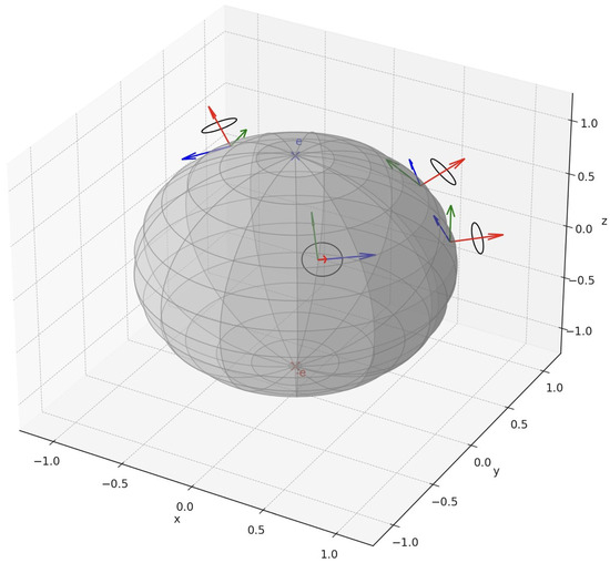
Figure 4. Principal $SO\left(2\right)$-bundle of oriented orthonormal frames over $M_e$.

7.2. Analysis of the Geometric Results

Every smooth orthonormal right-handed frame $f=(X,Y)$ on ${\mathbb{S}}^2\backslash \{e,-e\}$, satisfying $X\left(u\right)\times Y\left(u\right)=u$, is either:

• Equal to $f_e\left(u\right)=({\widehat{K}}_e\left(u\right),u\times {\widehat{K}}_e\left(u\right))$, or
• A rotation of $f_e$, i.e.,

  $$f\left(u\right)=(\rho \left(u\right){\widehat{K}}_e\left(u\right),\rho \left(u\right)(u\times {\widehat{K}}_e\left(u\right))),$$

  where

  $$\rho :{\mathbb{S}}^2\backslash \{e,-e\}\to SO\left(3\right)$$

  is a smooth rotation field satisfying

  $$\rho \left(u\right)u=u,$$

  effectively a rotation by a smooth angle $\theta \left(u\right)$ in $T_u{\mathbb{S}}^2$.

This result is interesting, as it shows that $f_e$ is a “standard” frame, and all other right-handed frames are obtained by rotating it in the tangent plane, reflecting the structure of the frame bundle and the symmetry of ${\mathbb{S}}^2$.

7.3. Analysis at the Boundary

All the functions, fields and frames we consider in the paper are defined upon open submanifolds of the sphere and of the dual of Minkowski space, considered as smooth manifolds in the standard Euclidean sense. Therefore, from a strictly analytical and differential geometry perspective, they can be very smooth without any reference to their possible compactifications and/or closures.

On the other hand, the study of such mappings at the Boundaries, poles or at singular planes, could be of a certain interest, from many points of view, and we indeed had conducted some related analysis from a topological point of view:

1.

For what concerns the frames and the unit vector fields, we have very few hopes of extensibility, because of the celebrated “hairy ball theorem”—we have literally a topological obstruction on the sphere at some inevitable “poles”—this means that at our boundaries, at the poles of our pierced spheres, the limits of such mappings could exist directionally, but, from each possible direction, we might obtain different limits, making it impossible to extend (continuously) from the pierced spheres to the entire sphere.

2.

The question is a little bit more subtle in the case of scalar smooth fields. We could have various scenarios; for example, in the case of our angular field $\theta$:

• We have cases in which such a smooth angular field can be extended smoothly to all of the sphere, for example, when the function is constant. However, even in this case, the existence of a global extension of $\theta$ cannot imply anything about the orientation of the Killing frame at the poles, because, at the pre-chosen poles, we will never be allowed to extend the Killing frame;
• We can construct examples in which the angular field shows various directional limits, at least two different limits coming from two convenient different directions;
• We can construct cases in which the limits at the poles could go to infinity.

Thus, we have all possible scenarios.

We insist, however, that the wildest possible behavior of the angular field at the poles does not damage, anyhow, the smoothness of the angular field on the open submanifold (pierced sphere) under examination.

8. Results IV: Orthonormal Right-Handed Frames on ${\mathbb{R}}^{\mathbf{3}}\backslash \mathbf{Span}\left\{\mathit{e}\right\}$

We have just proved that every smooth orthonormal right-handed frame on $S^2$, minus a prechosen e and its opposite $-e$, should be necessarily the Killing orthonormal frame $f_e$ or any of its rotation by a smooth rotation field $\rho :S^2\backslash \{e,-e\}\to SO\left(3\right)$.

Therefore, $f_e$ can be extended to the entire ${\mathbb{M}}_4^{*}\backslash {\mathsf{\Pi }}_e$ by homogeneity:

$${\tilde{f}}_e\left(k\right)=f_e\left({\displaystyle \frac{\mathbf{k}}{\left|\mathbf{k}\right|}}\right),$$

where ${\mathsf{\Pi }}_e$ is the linear plane generated by e and $(1,0,0,0)$.

Analogously, $f_e$ can be extended to the spatial part of ${\mathbb{M}}_4^{*}$ minus the straight-line generated by e.

Now, the following theorem holds.

Theorem 4. 

Every smooth orthonormal right-handed bidimensional frame

$$f:{\mathbb{R}}^3\backslash \mathit{span}\left\{e\right\}\to {\mathbb{R}}^3\times {\mathbb{R}}^3$$

—defined on ${\mathbb{R}}^3$ minus the line generated by a pre-chosen unit vector e—which is tangent at any point $\mathbf{k}$ to the sphere centered at the origin and passing by $\mathbf{k}$, should be necessarily ${\tilde{f}}_e$ (extension of $f_e$ to ${\mathbb{R}}^3$) or any of its rotations by a smooth rotation field

$$\rho :{\mathbb{R}}^3\backslash \mathit{span}\left\{e\right\}\to SO\left(3\right)$$

such that any rotation $\rho \left(\mathbf{k}\right)$ is a rotation with axis $\mathbf{k}$.

Theorem 4 is a natural generalization of Theorem 3, extending the concept of orthonormal right-handed frames from $S^2\backslash \{e,-e\}$ to ${\mathbb{R}}^3\backslash \mathrm{span}\left\{e\right\}$, where the frame is tangent to the sphere of radius $\left|\mathbf{k}\right|$ at each point $\mathbf{k}$. This connects directly to the homogeneous extension of $f_e$ to the Minkowski dual space ${\mathbb{M}}_4^{*}\backslash {\mathsf{\Pi }}_e$. Let us analyze Theorem 4 and verify its validity.

Theorem 3 follows from the triviality of the frame bundle over $S^2\backslash \{e,-e\}$, which is contractible.

8.1. Homogeneous Extension to ${\mathbb{M}}_4^{*}\backslash {\mathsf{\Pi }}_e$

The frame $f_e$ extends to ${\mathbb{M}}_4^{*}\backslash {\mathsf{\Pi }}_e$, where ${\mathsf{\Pi }}_e$ is the plane spanned by $(0,e)$ and $(1,0,0,0)$. For $k=(k^0,\mathbf{k})\in {\mathbb{M}}_4^{*}\backslash {\mathsf{\Pi }}_e$, $\mathbf{k}\ne 0$:

$${\tilde{f}}_e\left(k\right)=f_e\left({\displaystyle \frac{\mathbf{k}}{\left|\mathbf{k}\right|}}\right)=\left({\widehat{K}}_e\left(u\right),u\times {\widehat{K}}_e\left(u\right)\right),u={\displaystyle \frac{\mathbf{k}}{\left|\mathbf{k}\right|}}.$$

This is tangent to the sphere of radius $\left|\mathbf{k}\right|$ at $\mathbf{k}$.

8.2. Proof of Theorem 4

Proof of Theorem 4. 

Theorem 4 affirms that every smooth orthonormal right-handed frame

$$f:{\mathbb{R}}^3\backslash \mathrm{span}\left\{e\right\}\to {\left({\mathbb{R}}^3\right)}^2,$$

where $f\left(\mathbf{k}\right)=\left(X\right(\mathbf{k}),Y(\mathbf{k}\left)\right)$ is tangent to the sphere

$$S_{\left|\mathbf{k}\right|}=\{\mathbf{x}\in {\mathbb{R}}^3\mid \left|\mathbf{x}\right|=\left|\mathbf{k}\right|\},$$

is either ${\tilde{f}}_e\left(\mathbf{k}\right)$ or:

$$f\left(\mathbf{k}\right)=\left(\rho \left(\mathbf{k}\right){\widehat{K}}_e\left(u\right),\rho \left(\mathbf{k}\right)(u\times {\widehat{K}}_e\left(u\right))\right),$$

where $\rho \left(\mathbf{k}\right)\mathbf{k}=\mathbf{k}$. The frame f satisfies:

• Orthonormality. $X\left(\mathbf{k}\right)·X\left(\mathbf{k}\right)=Y\left(\mathbf{k}\right)·Y\left(\mathbf{k}\right)=1$, $X\left(\mathbf{k}\right)·Y\left(\mathbf{k}\right)=0$.
• Tangency. $X\left(\mathbf{k}\right)·\mathbf{k}=Y\left(\mathbf{k}\right)·\mathbf{k}=0$.
• Right-handedness. $X\left(\mathbf{k}\right)\times Y\left(\mathbf{k}\right)={\displaystyle \frac{\mathbf{k}}{\left|\mathbf{k}\right|}}$.

Analysis of Frame Bundle. At $\mathbf{k}$,

$$T_{\mathbf{k}}{S}_{\left|\mathbf{k}\right|}=\{\mathbf{v}\mid \mathbf{v}·\mathbf{k}=0\}.$$

The frame bundle of $S_{\left|\mathbf{k}\right|}$ is isomorphic to $SO\left(2\right)$. The bundle over ${\mathbb{R}}^3\backslash \mathrm{span}\left\{e\right\}$ may be non-trivial, as

$${\pi }_1({\mathbb{R}}^3\backslash \mathrm{span}\left\{e\right\})=\mathbb{Z},$$

but the condition $\rho \left(\mathbf{k}\right)\mathbf{k}=\mathbf{k}$ reduces the verification to the trivial bundle of $S_{\left|\mathbf{k}\right|}$.

Expressing the frame f as

$$X\left(\mathbf{k}\right)=cos\theta \left(\mathbf{k}\right){\widehat{K}}_e\left(u\right)+sin\theta \left(\mathbf{k}\right)(u\times {\widehat{K}}_e\left(u\right)),$$

$$Y\left(\mathbf{k}\right)=-sin\theta \left(\mathbf{k}\right){\widehat{K}}_e\left(u\right)+cos\theta \left(\mathbf{k}\right)(u\times {\widehat{K}}_e\left(u\right)),$$

where $\theta \left(\mathbf{k}\right)$ is smooth, the homogeneity reduces the problem to $S^2\backslash \{e,-e\}$, where the bundle is trivial, so Theorem 4 holds. □

Theorem 4 states that every considered frame is a radial rotation of ${\tilde{f}}_e$.

9. Results V: Maxwell–Schrödinger Fields from de Broglie Waves and Spherical Geometry

In this section, we present a foundational application of the spherical geometric structure and Killing frames developed above: a new construction of solutions to Maxwell’s equations in free space, formulated as a relativistic massless Schrödinger-type equation in the space of Schwartz-tempered complex vector distributions.

This construction unveils a one-to-one correspondence between light-like de Broglie wavevectors and exact Maxwellian solutions in the complexified Schwartz space

$$W={\mathcal{S}}^{\prime }({\mathbb{M}}_4,{\mathbb{C}}^3)=\mathcal{L}(\mathcal{S}({\mathbb{M}}_4,\mathbb{C}),{\mathbb{C}}^3)={\mathcal{S}}^{\prime }({\mathbb{M}}_4,\mathbb{C})\otimes {\mathbb{C}}^3,$$

revealing how quantum-phase distributions combine with polarization geometry to form a complete analytic model of free electromagnetic waves.

9.1. Minkowski Space, de Broglie Family, and Extended Frame Fields

The homogeneous extension of the aforementioned spherical frame ${\tilde{f}}_e$ can naturally embed into the wave vector space of Minkowski space-time ${\mathbb{M}}_4^{*}$ and thus construct electromagnetic solutions in conjunction with de Broglie waves from quantum mechanics.

Let ${\mathbb{M}}_4={\mathbb{R}}_{1,3}$ denote Minkowski space-time, and ${\mathbb{M}}_4^{*}$ its dual (space of real 4-wavevectors). A wavevector $k=(k^0,\overrightarrow{k})\in {\mathbb{M}}_4^{*}$ induces the tempered de Broglie phase:

$${\eta }_k:=\left[e^{i⟨k,x⟩}\right]=[e^{i(\overrightarrow{k}·\overrightarrow{x}-{\omega }_{k}t)}], \mathrm{with} {\omega }_k=c{k}^0.$$

This defines a scalar tempered wave distribution in the canonical way, x is the canonical coordinate on Minkowski vector space (identity mapping), $t=x^0/c$ is the time coordinate of x (time projection), $\overrightarrow{x}$ is the space projection of the identity chart x, $\left[g\right]$ is the tempered distribution associated with any smooth slowly increasing (multiplier) function g (see Figure 5).

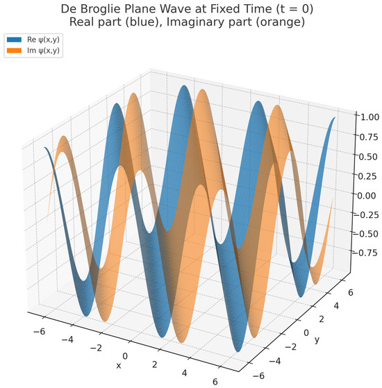
Figure 5. De Broglie plane wave at fixed time ($t=0$).

To construct complex vector fields, we extend the Killing frame

$$f_e=({\overrightarrow{r}}_e,{\overrightarrow{s}}_e)$$

from the sphere $S^2\backslash \{\pm e\}$ to the dual Minkowski space ${\mathbb{M}}_4^{*}\backslash {\mathsf{\Pi }}_e$ by homogeneity:

$${\overrightarrow{u}}_k={\displaystyle \frac{\overrightarrow{k}}{|\overrightarrow{k}|}},{\overrightarrow{r}}_k:={\widehat{K}}_e\left({\overrightarrow{u}}_k\right)={\displaystyle \frac{e\times {\overrightarrow{u}}_k}{|e\times {\overrightarrow{u}}_k|}},{\overrightarrow{s}}_k:={\overrightarrow{u}}_k\times {\overrightarrow{r}}_k.$$

This defines a smooth, orthonormal, right-handed frame $({\overrightarrow{r}}_k,{\overrightarrow{s}}_k,{\overrightarrow{u}}_k)$ for each $k\notin {\mathsf{\Pi }}_e$, where ${\mathsf{\Pi }}_e$ is the singular plane generated by e and $(1,0,0,0)$.

We define the complex polarization vector associated with k:

$${\overrightarrow{f}}_k:={\overrightarrow{r}}_k+i{\overrightarrow{s}}_k\in {\mathbb{C}}^3,$$

and the corresponding complex plane field associated with k:

$$w_k:={\eta }_k.{\overrightarrow{f}}_k=\left[e^{i(\overrightarrow{k}·\overrightarrow{x}-\omega t)}\right].({\overrightarrow{r}}_k+i{\overrightarrow{s}}_k)\in {\mathcal{S}}^{\prime }({\mathbb{M}}_4,{\mathbb{C}}^3).$$

This defines a Schwartz family w of plane-wave complex 3-field distribution parameterized by all 4-wavevectors $k\in {\mathbb{M}}_4^{*}\backslash {\mathsf{\Pi }}_e$ (see Figure 6).

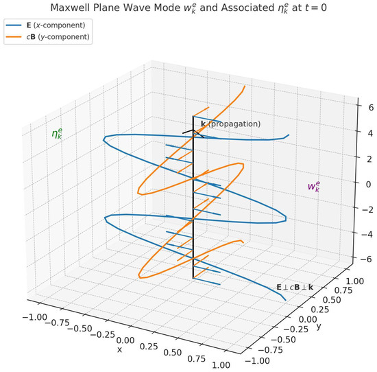
Figure 6. Maxwell plane wave mode $w_k^e$ and associated ${\eta }_k^e$ at $t=0$.

9.2. The Maxwell–Schrödinger Equation on ${\mathcal{S}}^{\prime }({\mathbb{M}}_4,{\mathbb{C}}^3)$

Let us now consider the Maxwell–Schrödinger equation, defined on the full space of tempered complex vector distributions:

$$i{\displaystyle \frac{\partial F}{\partial t}}=c\nabla \times F.$$

This equation arises from the classical Maxwell curl equations in free space, under the complexification

$$F:=\overrightarrow{E}+ic\overrightarrow{B}.$$

Proof. 

Indeed, the two Maxwell curl equations:

$$c\nabla \times \overrightarrow{E}=-{\displaystyle \frac{\partial \left(c\overrightarrow{B}\right)}{\partial t}},c\nabla \times \left(c\overrightarrow{B}\right)={\displaystyle \frac{\partial \overrightarrow{E}}{\partial t}}$$

combine into the single complex equation above:

$$i{\displaystyle \frac{\partial (\overrightarrow{E}+ic\overrightarrow{B})}{\partial t}}=c\nabla \times (\overrightarrow{E}+ic\overrightarrow{B}).$$

It is enough to multiply the second equation

$$c\nabla \times \left(c\overrightarrow{B}\right)={\displaystyle \frac{\partial \overrightarrow{E}}{\partial t}},$$

times the imaginary unit i and add the first equation in the form

$$c\nabla \times \overrightarrow{E}=i{\displaystyle \frac{\partial \left(ic\overrightarrow{B}\right)}{\partial t}}.$$

As we desired. □

Importantly, this evolution equation is always defined on

$$W={\mathcal{S}}^{\prime }({\mathbb{M}}_4,{\mathbb{C}}^3),$$

independent of any constraint on the wavevector k.

This complex equation form compresses the classical Maxwell equations into a single evolution equation (derivation can be found just above) and allows for the unified treatment of singularities and quantum phases in the distribution space ${\mathcal{S}}^{\prime }$, providing a framework for subsequent spectral analysis.

We observe that by choosing the complex form of Maxwell’s equations, we establish that the natural space of Maxwell’s electromagnetism is the tempered field space $W={\mathcal{S}}^{\prime }({\mathbb{M}}_4,{\mathbb{C}}^3)$; this space is the tensor product of ${\mathcal{S}}^{\prime }({\mathbb{M}}_4,\mathbb{C})\otimes {\mathbb{C}}^3$. This simple decomposition discloses the direct link between the quantum wave space and Maxwell’s field space.

9.3. The General Plane Wave Family

Each tempered field

$$w_k={\eta }_k.{\overrightarrow{f}}_k$$

is well-defined for any $k\in {\mathbb{M}}_4^{*}\backslash {\mathsf{\Pi }}_e$, and constitutes (when viewed as a function) a smooth slowly increasing polarized complex plane wave.

• We shall consider, mainly, the entire smooth family

  $$w:{\mathbb{M}}_4^{*}\backslash {\mathsf{\Pi }}_e\to W.$$

Remark 1. 

As usual in Schwartz linear algebra (and in quantum mechanics), we are searching for an entire (possibly orthonormal) eigenbasis of some observable in order to decompose every state of the system as a superposition of that basis. In our specific case, w shall diagonalize every differential operator and every linear combination of those operators as soon as they are defined upon the Schwartz linear span $S_w$ of w. Energy and momentum operators in $S_w$ will be diagonalized by w; furthermore, even more notably for our present study, w shall diagonalize the curl operator, which is the dynamic leading operator of Maxwell’s equation. The operator curl restricted to $S_w$ and multiplied by Plank’s constant shall reveal the momentum magnitude operator of quantum mechanics.

The member fields of w are:

• Globally defined tempered vector distributions;
• Solenoidal:

  $$\nabla ·w_k=0,$$

  since $\overrightarrow{k}·{\overrightarrow{f}}_k=0$;
• Eigenfunctions of all differential operators, and in particular:

  $$\nabla \times w_k=\left|\overrightarrow{k}\right|w_k,$$

  since $\overrightarrow{u}\times {\overrightarrow{f}}_k=-i{\overrightarrow{f}}_k$;
• Time-evolved by the eigenvalue equation:

  $$i{\displaystyle \frac{\partial w_k}{\partial t}}={\omega }_k{w}_k=c{k}^0{w}_k.$$

Thus, for all $k\notin {\mathsf{\Pi }}_e$, the fields $w_k$ are dynamically meaningful—but only a subfamily solves the (massless) Maxwell–Schrödinger equation.

9.4. The Maxwell Characterization Theorem

We now formally isolate the subfamily of physically admissible Maxwellian (massless) fields.

Theorem 5 

(Maxwellian Electromagnetic Solutions Characterization). Let

$$k\in {\mathbb{M}}_4^{*}\backslash {\mathsf{\Pi }}_e,$$

and define the complex plane wave field

$$w_k={\eta }_k.({\overrightarrow{r}}_k+i{\overrightarrow{s}}_k).$$

Then, the field $w_k$ satisfies the Maxwell–Schrödinger equation (in free space)

$$i{\displaystyle \frac{\partial w_k}{\partial t}}=c\nabla \times w_k$$

if and only if the wavevector k is light-like and ${\omega }_k>0$, i.e.,

$$k^0>0,⟨k,k⟩=-{\left(k^0\right)}^2+{\left|\overrightarrow{k}\right|}^2=0.$$

Proof. 

We have:

$$i{\displaystyle \frac{\partial w_k}{\partial t}}={\omega }_k{w}_k,\nabla \times w_k=\left|\overrightarrow{k}\right|w_k.$$

Then the Maxwell–Schrödinger equation reads:

$${\omega }_k{w}_k=c|\overrightarrow{k}|w_k⟺{\omega }_k=c\left|\overrightarrow{k}\right|,$$

which holds if and only if $k^0=\left|\overrightarrow{k}\right|$, i.e., $⟨k,k⟩=0$. □

9.5. Physical and Structural Implications

This result underscores the structure of the full family $w={\left(w_k\right)}_{k\in {\mathbb{M}}_4^{*}\backslash {\mathsf{\Pi }}_e}$:

• All $w_k$ are smooth complex polarized plane fields with well-defined dynamics;
• Only those with light-like k solve the massless Maxwell–Schrödinger equation and hence represent bona fide electromagnetic fields in vacuum;
• The Maxwell’s equation in free space

  $$i{\partial }_{t}F=c\nabla \times F$$

  thus functions as a spectral filter, selecting light-cone indexed de Broglie fields;
• The Maxwell complex equation coincides with the relativistic Schrodinger equation for massless particles upon $S_w$;
• We underline that the fields $w_k$ represent electromagnetic fields only in free space, as its real and imaginary parts are mutually orthogonal.

This filtering highlights the deep unity of geometry (through the Killing-induced frame), spectral phase and quantum mechanics (via the de Broglie basis $\eta$ and the associated diagonalizable operators on it), and field dynamics (via the curl operator) within the Maxwell–Schwartz formalism.

9.6. Why Introduce Schwartz Distributions?

That is one of the core points of the entire approach. It could seem we have intended only to extend the set of all possible quantum states and solutions, that is not at all bad, per se, and from an applicative perspective, but the motivations are deeper and profoundly structural. We do not want here to introduce all the great and numerous advantages of the Schwartz space of tempered distributions in quantum mechanics ([30]), or of Rigged Hilbert space Theory ([31,32,33]) or of general Schwartz linear algebra ([34,35,36,37,38]), but strictly we try to limit the justification to the specific content of the paper:

1.

The basic quantum states ${\eta }_k$, we consider heavily in the paper, are de Broglie waves, which are smooth “slowly increasing” functions and not at all square-integrable in the standard Lebesgue sense. They are, naturally, tempered distributions. They do not belong, in their totality, to any reasonably conceivable separable Hilbert space.

2.

The de Broglie family $\eta$ is a Schwartz basis of the entire space of complex tempered distributions; it is of fundamental importance to extend, linearly and continuously, any operator defined upon $\eta$, for instance to construct our topological isomorphism between the solution space of a relativistic Schrödinger equation and that of our generalized Maxwell’s equations;

3.

Any differential operator on the space of tempered distributions is defined everywhere, linearly and continuously, and also in tempered field space, so that the fundamental equations (Schrödinger and Maxwell’s) are linear continuous operator-equations;

4.

Any differential operator is Schwartz diagonalizable by the eta basis, which guarantees the possibility of an extremely efficient and applicable functional calculus, which, among other things, allows for the definition of the principal square root of the real positive differential operators;

5.

The possibility to define correctly and efficiently the square roots of linear continuous operators follows from the very strong formulation of the spectral theory in tempered distribution spaces, and this allows us to define the general relativistic Schrödinger equation and the generalized massive Maxwell’s equations.

9.7. Why Choose the Complex Field Equation $i{\partial }_{t}F=c\nabla \times F?$

Apparently, the complex version just summarizes the four Maxwell’s equations to only two. More importantly, Maxwell’s curl equations become the unique Schrödinger-like equation above, which, on the (very vast) subspace generated by the family w, is exactly the relativistic massless Schrödinger equation

$$i\hslash {\partial }_{t}F=c\left|P\right|F,$$

We soon realized that (in complex tempered field space generated by our family w) the fundamental linear continuous operators $\hslash \nabla \times$ and $\left|P\right|$ (the magnitude of momentum operator, defined spectrally on the subspace generated by w) are indeed the same operator.

This is true and meaningful in tempered Schwartz spaces but not in Hilbert spaces or other affiliates environments.

The coincidence of the two fundamental operators, from Maxwell’s electromagnetism and quantum mechanics Schrödinger’s picture, is of critical importance to unifying (at least in a great deal of cases) the two theories, and it allows to extend the above-mentioned Maxwell’s field equation to the new massive case. From a purely mathematical point of view, it is almost superfluous to observe that differential equations, pseudo-differential equations and fractional differential equations find their most favorable environment in distributions spaces.

10. Results VI: Massive Maxwellian Fields and the Relativistic Maxwell–Schrödinger Equation

We now extend the previous theory from massless electromagnetic fields to a broader class of massive Maxwellian fields governed by the relativistic Hamiltonian for nonzero rest mass $m_0$. We desire to underline that the massive field does not mean at all a material field. This framework generalizes the light-cone condition

$$⟨k,k⟩=0$$

to the mass shell condition

$$⟨\hslash k,\hslash k⟩=-{\left(m_{0}c\right)}^2,$$

preserving the complex geometric structure and eigenbasis of the Maxwell–Schrödinger formalism.

The fundamental idea is to replace the linear continuous light-photon Hamiltonian operator

$${\widehat{H}}_0=c\left|\overrightarrow{P}\right|=c\hslash \nabla \times ,$$

considered as restricted on the de Broglie Killing subspace $S_w$, with the relativistic Hamiltonian operator

$${\widehat{H}}_{m_0}=c\sqrt{{(\hslash \nabla \times )}^2+{\left(m_{0}c\right)}^2{\mathbb{I}}_W},$$

defined again, spectrally, on the de Broglie–Killing subspace

$$S_w\subset W={\mathcal{S}}^{\prime }({\mathbb{M}}_4,{\mathbb{C}}^3),$$

Schwartz-generated by w.

10.1. Momentum Magnitude Operator and Spectral Identification with Curl

Recall that in Section 9, the space $S_w$ is defined as the Schwartz linear span of the de Broglie–Killing family $w={\left(w_k\right)}_{k\in D}$,

$$S_w=\left\{{\int }_{D}aw\in W:a\in {\mathcal{S}}^{\prime }({\mathbb{M}}_4^{*},\mathbb{C}),supp\left(a\right)\cap {\mathsf{\Pi }}_e=\varnothing \right\}.$$

On this subspace, the operator $|\overrightarrow{P}|$ is defined spectrally by:

$$|\overrightarrow{P}|\left({\int }_{D}aw\right):={\int }_{D}a(\hslash |\overrightarrow{\mathrm{k}}\left|\right)w,$$

whenever a vanishes in a neighborhood of the singular plane ${\mathsf{\Pi }}_e$ and where $\overrightarrow{\mathrm{k}}$ is the spatial projection in ${\mathbb{M}}_4^{*}$. This operator is well-defined on a large domain of test functions whose Fourier transforms vanish along the line generated by $(1,0,0,0)$.

Now observe that the complex vector-field family w is an eigenbasis of $S_w$ for both the operator $|\overrightarrow{P}|$ and the scaled curl operator $\hslash \nabla \times$, with matching eigenvalues:

$$|\overrightarrow{P}|\left(w_k\right)=\hslash |\overrightarrow{k}|·w_k,\hslash \nabla \times w_k=\hslash \left|\overrightarrow{k}\right|·w_k.$$

Therefore, we conclude that the above two operator restrictions upon the subspace $S_w$ coincide:

$$|\overrightarrow{P}{|}_{|S_w}={(\hslash \nabla \times )}_{|S_w},$$

since the two operators are spectrally identical on $S_w$.

10.2. Quantization of the Relativistic Hamiltonian

The usual relativistic Hamiltonian of a free particle with rest mass $m_0$ is:

$$H_{m_0}\left(\overrightarrow{p}\right)=c\sqrt{|\overrightarrow{p}{|}^2+{\left(m_{0}c\right)}^2}.$$

Its quantization on the space W can be performed by applying the Schwartz spectral theorem to the self-adjoint operator $|\overrightarrow{P}|$ defined on $S_w$, yielding:

$${\widehat{H}}_{m_0}:=c\sqrt{|\overrightarrow{P}{|}^2+{\left(m_{0}c\right)}^2{\mathbb{I}}_W}=c\sqrt{{(\hslash \nabla \times )}^2+{\left(m_{0}c\right)}^2{\mathbb{I}}_W},$$

with ${\mathbb{I}}_W$ the identity operator on W (if we desire to strictly restrict our attention to $S_w$, we can clearly use the identity operator of the latter subspace). On the basis w, we obtain, by the very definition of our Hamiltonian operator (via Schwartz spectral theorem):

$${\widehat{H}}_{m_0}\left(w_k\right)=c\sqrt{(\hslash |\overrightarrow{k}{\left|\right)}^2+{\left(m_{0}c\right)}^2}.w_k=H_{m_0}(\hslash \overrightarrow{k}).w_k.$$

Thus, the family w diagonalizes the relativistic Hamiltonian ${\widehat{H}}_{m_0}$.

The complete definition of Hamiltonian operator ${\widehat{H}}_{m_0}$ on $S_w$ is given by superpositions:

$${\widehat{H}}_{m_0}\left({\int }_{D}aw\right):={\int }_{D}ac\sqrt{(\hslash |\overrightarrow{\mathrm{k}}{\left|\right)}^2+{\left(m_{0}c\right)}^2}.w,$$

whenever a vanishes in a neighborhood of the singular plane ${\mathsf{\Pi }}_e$ and where $\overrightarrow{\mathrm{k}}$ is the spatial projection in ${\mathbb{M}}_4^{*}$. In a perfectly equivalent way, we can write

$${\widehat{H}}_{m_0}\left(F\right):={\int }_{D}c\sqrt{(\hslash |\overrightarrow{\mathrm{k}}{\left|\right)}^2+{\left(m_{0}c\right)}^2}.{\left(F\right)}_{w}w,$$

where ${\left(F\right)}_w$ is the representation of any $F\in S_w$ in the basis w (the coefficient distribution a above).

Remark 2. 

It is worthy now to observe that we can project any complex vector distribution 3-field F of $S_w$ onto a scalar complex wave distribution ${\psi }_F$ by the following homomorphism:

$$\psi :S_w\to {\mathcal{S}}^{\prime }({\mathbb{M}}_4,\mathbb{C}):F\mapsto {\int }_D{\left(F\right)}_w\eta .$$

10.3. The Relativistic Maxwell–Schrödinger Equation

We now consider the massive Maxwell–Schrödinger evolution equation:

$$i\hslash {\displaystyle \frac{\partial F}{\partial t}}={\widehat{H}}_{m_0}\left(F\right),$$

where $F\in S_w$ and ${\widehat{H}}_{m_0}$ is defined above.

Each field

$$w_k=\left[e^{i(\overrightarrow{k}·\overrightarrow{x}-{\omega }_{k}t)}\right].({\overrightarrow{r}}_k+i{\overrightarrow{s}}_k)$$

is (as we already know) a complex plane vector distribution in W and satisfies:

$$i\hslash {\displaystyle \frac{\partial w_k}{\partial t}}=(\hslash {\omega }_k)w_k.$$

On the other hand, by definition of ${\widehat{H}}_{m_0}$:

$${\widehat{H}}_{m_0}\left(w_k\right)=H_{m_0}(\hslash \overrightarrow{k})w_k=c\sqrt{(\hslash |\overrightarrow{k}{\left|\right)}^2+{\left(m_{0}c\right)}^2}{w}_k.$$

10.4. Characterization Theorem for Massive Maxwellian Fields

We now isolate the subfamily of massive plane-wave solutions that satisfy the relativistic Maxwell–Schrödinger equation above.

Theorem 6 

(Massive Maxwellian Solutions Characterization). Let us consider any 4-wavevector $k\in {\mathbb{M}}_4^{*}\backslash {\mathsf{\Pi }}_e$, and let

$$w_k:={\eta }_k.({\overrightarrow{r}}_k+i{\overrightarrow{s}}_k)$$

be the Schwartz Killing basis member as defined above. Then, the complex tempered vector field $w_k$ satisfies the free space relativistic Maxwell–Schrödinger equation

$$i\hslash {\displaystyle \frac{\partial F}{\partial t}}={\widehat{H}}_{m_0}\left(F\right)$$

if and only if $k^0>0$ and

$$⟨\hslash k,\hslash k⟩=-{\left(m_{0}c\right)}^2,$$

that is, if and only if

$$\hslash {\omega }_k=H_{m_0}(\hslash \overrightarrow{k})=c\sqrt{(\hslash |\overrightarrow{k}{\left|\right)}^2+{\left(m_{0}c\right)}^2}.$$

Proof. 

Substituting $w_k$ in the equation, at the place of the unknown F, the left-hand side of the equation becomes

$$i\hslash {\partial }_t{w}_k=\hslash {\omega }_k·w_k.$$

Analogously, the right-hand side becomes

$${\widehat{H}}_{m_0}\left(w_k\right)=c\sqrt{(\hslash |\overrightarrow{k}{\left|\right)}^2+{\left(m_{0}c\right)}^2}·w_k.$$

These tempered fields are equal if and only if ${\omega }_k$ is positive and

$$\hslash {\omega }_k=c\sqrt{(\hslash |\overrightarrow{k}{\left|\right)}^2+{\left(m_{0}c\right)}^2}⟺-{(\hslash {\omega }_k/c)}^2+(\hslash |\overrightarrow{k}{\left|\right)}^2=-{\left(m_{0}c\right)}^2,$$

which is the condition

$$⟨\hslash k,\hslash k⟩=-{\left(m_{0}c\right)}^2.$$

Exactly as we desired. □

In a perfect symmetrical fashion, we could define the conjugate Maxwell–Schrodinger equation (opposite time coordinate) for antimatter fields ($\omega <0$) and prove the analogous theorem. We left the details to the reader.

10.5. Discussion and Physical Relevance

This result shows that the family w parameterizes not only massless (photon-like) wave solutions, but also massive complex vector fields governed by the relativistic energy-momentum relation:

$$E^2=\left(\right|\overrightarrow{p}{\left|c\right)}^2+{\left(m_0{c}^2\right)}^2.$$

In this broader framework:

• The relativistic Maxwell Schrodinger operator ${\widehat{H}}_{m_0}$ extends the massless Maxwell’s Hamiltonian operator ${\widehat{H}}_0=c\left|\overrightarrow{P}\right|$ to include rest mass $m_0$ different from 0;
• The fields $w_k$ with $k^0>0$ and

  $$⟨\hslash k,\hslash k⟩=-{\left(m_{0}c\right)}^2$$

  form a spectral submanifold of $S_w$ determined by ${\widehat{H}}_{m_0}$ via the associated Maxwell Schrodinger equation; the case with $k^0<0$ is covered analogously by the conjugate equation;
• This construction generalizes Maxwell’s electromagnetic fields to a class of massive relativistic Maxwell-like fields within Schwartz-tempered complex vector theory.

The structure suggests that the space $S_w$ may serve as a host for a unified field-theoretic framework accommodating both massless and massive quantum fields via geometry and spectral analysis alone.

11. Conclusions and Outlook

This work has established a geometric, analytic, and physical synthesis centered on the role of orthonormal right-handed frames derived from Killing vector fields on the two-sphere ${\mathbb{S}}^2$, and their application to constructing explicit solutions of Maxwell’s equations in free-space and their massive generalizations.

In the first part of the paper, we rigorously developed the mathematical framework in which smooth orthonormal right-handed tangent frames on the pierced sphere ${\mathbb{S}}^2\backslash \{\pm e\}$ are constructed canonically from the action of the rotation group $\mathrm{SO}\left(3\right)$ and its Lie algebra $\mathfrak{so}\left(3\right)$. We proved that every such frame is either a Killing frame $f_e$ or any its rotation by a smooth field of elements in $\mathrm{SO}\left(3\right),$ pointwise fixing the direction u orthogonal to the tangent space generated by the frame at any point u. This characterization aligns the local geometry of the sphere with the global topology of its frame bundle and sets the stage for a frame-theoretic approach to field equations.

Building upon this geometry, we then transitioned to the realm of Schwartz-tempered complex vector fields on Minkowski space-time, introducing the fundamental Schwartz basis w of complex plane wave solutions. The fields $w_k$ are constructed by lifting the de Broglie plane wave

$${\eta }_k=\left[e^{i⟨k,x⟩}\right]$$

with a smoothly extended orthonormal frame adapted to the spatial direction of k. Each $w_k$ encodes both the phase propagation and polarization structure of an electromagnetic mode.

In Section 9, we demonstrated that the Maxwell curl equations in a vacuum admit an elegant reformulation as a single Schrödinger-type equation:

$$i{\partial }_{t}F=c\nabla \times F,$$

defined on the space $W={\mathcal{S}}^{\prime }({\mathbb{M}}_4,{\mathbb{C}}^3)$. Any basis field $w_k$ satisfies this equation if and only if the wavevector k is light-like, i.e., $⟨k,k⟩=0$. This result introduces a precise spectral filtering: the Maxwell–Schrödinger operator selects the light cone in dual Minkowski space as the physical support of radiation fields. In this free space setting, the real and imaginary parts of $w_k$ are uniformly proportional, respectively, to the electric and magnetic components of a circularly polarized wave $(E,cB)$. Any pair

$$(E,cB)=|E_0|w_k,$$

represents a legitimate electromagnetic field and a legitimate quantum wave field in W, whose associated complex Schrödinger wave is the wave distribution

$${\psi }_{(E,cB)}=\left|E_0\right|{\eta }_k.$$

In this sense, we reconsider the rightful place of wave amplitudes. The waves carry a natural physics meaning: as in the proper electromagnetic ones, the amplitudes stand for the intensity of the fields (as it is obvious and natural); the superposition principle holds in its whole glory (that is, within a fully functioning vector space structure and not in some fancy and sloppy projective Hilbert space). Of course, with any conveniently normalizable $\psi$, we can associate its “complex probability amplitude wave” ${\psi }^s/\left|\right|{\psi }^s\left|\right|$, where ${\psi }^s$ is the spatial tensor factor of $\psi$, assuming $\psi$ is tensorially decomposable as the tensor product of two distributions ${\psi }^t$ and ${\psi }^s$ depending separately on time and space, respectively. This association of a probability distribution to a state $\psi$ is particularly efficient and natural in distribution spaces, since probability measures are distribution-like objects and since distribution spaces contain all possible pre-Hilbert spaces of normalizable space-dependent distributions adopted in quantum mechanics.

In Section 10, we have extended the formalism to encompass massive Maxwellian fields, introducing the relativistic Hamiltonian

$${\widehat{H}}_{m_0}=c\sqrt{{(\hslash \nabla \times )}^2+{\left(m_{0}c\right)}^2{\mathbb{I}}_W},$$

and establishing that the fields $w_k$ satisfy the relativistic evolution equation

$$i\hslash {\displaystyle \frac{\partial F}{\partial t}}={\widehat{H}}_{m_0}\left(F\right)$$

if and only if the momentum-energy vector $\hslash k$ lies on the mass shell:

$$k^0>0,⟨\hslash k,\hslash k⟩=-{\left(m_{0}c\right)}^2.$$

This result generalizes the light cone condition to arbitrary mass, while preserving the geometry and spectral structure developed in the massless case.

At the heart of this theory lies the profound observation that the Maxwellian operator

$$\hslash \nabla \times :W\to W,$$

originally arising from classical electrodynamics, coincides with the quantum mechanical momentum magnitude operator $|\overrightarrow{P}|$ on the Schwartz span $S_w$ of any possible de Broglie–Killing basis w. This spectral identity reveals a hidden quantum-geometric unification: the Maxwell fields, their associated de Broglie waves, and the relativistic Hamiltonian structure are all bound together by the common Killing eigenbases w.

• Outlook. The physical unification developed here suggests several promising directions:

• A refined theory of electromagnetic wave packets as tempered superpositions of $w_k$ modes, localized in energy and direction.
• Extensions to curved space-time using local frames built from generalizations of Killing fields.
• Applications to gauge theories, where frame fields and group actions play a central role.
• Exploration of probability amplitudes and current densities associated with the massive fields $w_k$, with potential links to quantum optics and relativistic quantum information.

In all these developments, the frame-theoretic and spectral foundation laid out in this paper offers a powerful and unifying viewpoint. The tempered complex field space W emerges as a natural host for both classical and quantum electrodynamics, governed by a geometry of symmetry, polarization, and spectral evolution.

From Maxwell Electrodynamics to Relativistic Quantum Mechanics by Lie Algebra Transition

Passing from Maxwell electrodynamics to relativistic quantum mechanics is encoded by passing from the Lie algebra (it is a Lie algebra isomorphic to $({\mathbb{R}}^3,\times )$) $\mathfrak{so}\left(3\right)$ of Killing vector fields on the 2-sphere to the Lie algebra (it is a Lie algebra isomorphic to $(\mathbb{R},[,\left]\right)$ with trivial null brackets) $\mathfrak{so}\left(2\right)$ of the space of killing vector fields on the complex plane.

• How exactly do we pass from the Maxwell picture to the Schrödinger picture?
• Let us consider the following diagram, which defines exactly the “passage” (projection)

  $${\mathsf{\Psi }}^e:S^{\prime }{({\mathbb{M}}_4,{\mathbb{C}}^3)}_e\to S^{\prime }{({\mathbb{M}}_4,\mathbb{C})}_e$$

  from Maxwell’s space to quantum mechanics tempered distribution space:

  $${\mathsf{\Psi }}^e:F=(\overrightarrow{E},c\overrightarrow{B})=A{w}_k^e=A{\eta }_k^e.f_k^e\mapsto A{\eta }_k^e.1,$$

  for every k in the dual ${\mathbb{M}}_4^{*}$ and every real amplitude A:
• our projection ${\mathsf{\Psi }}^e$ replaces the orthonormal Killing frame $f^e$, which perfectly represents both the geometry of the Killing vector fields and the geometry/configuration/polarization of the electromagnetic field F, with the constant orthonormal frame $\left(1\right)$, which is mono-dimensional since $\mathfrak{so}\left(2\right)$ is monodimensional (see Figure 7).
  

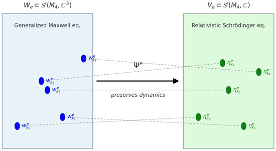  Figure 7. Isomorphism ${\mathsf{\Psi }}^e$ from Maxwell field subspace to scalar wave subspace.

Observe that the construction of this projection ${\mathsf{\Psi }}^e$ is extremely charged of physical content: in the fundamental complex product

$${\eta }_k^e.f_k^e$$

we find the dynamics of quantum mechanics (de Broglie waves) and the geometry of Maxwell electromagnetism, mixed together in order to shape a linear continuous isomorphism ${\mathsf{\Psi }}^e$ between two extremely vast subspaces of $S^{\prime }({\mathbb{M}}_4,{\mathbb{C}}^3)$ and $S^{\prime }({\mathbb{M}}_4,\mathbb{C})$, respectively, such that any electromagnetic-like field $F\in dom\left({\mathsf{\Psi }}^e\right)$ of the Schwartz linear span of $w^e$ satisfies the $m_0$-massive Maxwell’s complex equations iff its mirroring image ${\mathsf{\Psi }}^e\left(F\right)$ satisfies the $m_0$-massive relativistic Schrödinger’s equation. The circle is closed because our continuous linear isomorphism establish a strong bijective correspondence between the solutions of the two governing fundamental equations of the two respective spaces.

Referee suggestion. The theory of non-commutative differential calculi enables us to formulate differential geometries on the basis of chains of complexes of Lie algebras and one of the referees suggests to lift the reformulation of the above remark onto the level of non-commutative differential geometries corresponding to $\mathfrak{so}\left(2\right)$ and $\mathfrak{so}\left(3\right)$. The resulting non-commutative differential geometries could better clarify the transition from classical mechanics of Maxwell electrodynamics to its special relativity extension (from our perspective) and then proceed to the extension of the results of this work to QED and Abelian gauge theories.

Appendix A.1. Rotational Dynamics and Related Physical Example

“Rotational dynamics” refers to the dynamics governed by rotational symmetries, e.g., angular momentum conservation, also in electromagnetism.

Definition A1. 

Rotational dynamics here denotes the physical, dynamical processes invariant under the group $SO\left(3\right)$ of spatial rotations, such as the propagation of electromagnetic waves in isotropic space.

For instance, the precession of magnetic moments in a uniform field.

Appendix A.2. Geometric Symmetries in Quantum Mechanics

While our way of using Killing vector fields in quantum mechanics is completely original (and then we cannot find anything strictly similar in literature), Killing vector fields are fundamental objects in differential geometry that preserve the metric tensor of a Riemannian (or pseudo-Riemannian) manifold under the Lie derivative. They generate continuous symmetries (isometries) of the manifold, such as rotations or translations. In the context of physics, these symmetries lead to conserved quantities via Noether’s theorem in classical mechanics.

In quantum mechanics (QM), angular momentum operators

$$L_x,L_y,L_z$$

or collectively

$$\mathbf{L},$$

are Hermitian operators on the Hilbert space

$$L^2\left({\mathbb{R}}^3\right)$$

that generate rotations in a typical operator sense. They satisfy the commutation relations

$$[L_i,L_j]={ϵ}_{ijk}{L}_k,$$

and they generate a Lie algebra, with respect to the addition, real scalar multiplication and commutation brackets, isomorphic to

$$\mathfrak{su}\left(2\right)\cong \mathfrak{so}\left(3\right),$$

mirroring the algebra of rotations, as done by the Lie algebra of Killing vector fields. These operators arise from quantizing classical angular momentum, which is conserved due to rotational invariance. The connection between Killing vector fields and angular momentum operators in QM is through geometric quantization and the representation of symmetries.

Appendix A.2.1. Classical Level

On manifolds like ${\mathbb{R}}^3$ (flat space) or ${\mathbb{S}}^2$ (unit sphere), Killing vector fields generate rotational symmetries. For example, on ${\mathbb{R}}^3$ with the Euclidean metric, the rotational Killing fields are defined by

$$K_x=y{\partial }_z-z{\partial }_y,K_y=z{\partial }_x-x{\partial }_z,K_z=x{\partial }_y-y{\partial }_x,$$

where $x,y,z$ are the standard projections of the space. Their Lie brackets satisfy

$$[K_i,K_j]={ϵ}_{ijk}{K}_k,$$

and the Lie algebra generated by them is isomorphic to $\mathfrak{so}\left(3\right).$ On ${\mathbb{S}}^2,$ the three independent Killing fields also span $\mathfrak{so}\left(3\right),$ generating the rotation group $SO\left(3\right)$, by exponentiation.

Appendix A.2.2. Quantization

In QM, these classical symmetries are promoted to operators. The orbital angular momentum operators are obtained by quantizing the Poisson brackets of the classical functions associated with these Killing fields (e.g., via the correspondence principle, replacing classical variables with operators and Poisson brackets with commutators). Explicitly, the operator corresponding to $K_x$ is

$$L_x=-i\hslash (y{\partial }_z-z{\partial }_y),$$

and similarly for others. We observe the perfect formal similarity with the differential manifold version of Killing vector fields when using the partial derivative tangent frame $({\partial }_x,{\partial }_y,{\partial }_z).$ This is part of geometric quantization, where prequantum operators are defined on sections of a line bundle over the phase space, and Killing fields provide the momentum maps for symmetries.

Appendix A.2.3. On Curved Manifolds

The relation extends to curved spaces, where momentum operators can be defined using Killing vector fields whose integral curves are geodesics (straight lines in curved geometry). For instance, on spaces of constant curvature (like the sphere), these operators generalize linear momentum and angular momentum, ensuring hermiticity and compatibility with the manifold’s geometry. This is crucial for quantum systems on curved backgrounds, such as in quantum gravity or condensed matter models.

Appendix A.2.4. Physical Implications

In atomic physics or quantum optics, angular momentum operators describe rotational states, e.g., spherical harmonics as eigenfunctions on ${\mathbb{S}}^2$. The Killing fields underlie the classical symmetries that quantize to these operators, unifying geometry with quantum symmetries. This bridge is a cornerstone of how classical geometric symmetries manifest in quantum theory, often explored in texts on quantum mechanics on manifolds or Lie group representations.

Appendix A.3. Lie Algebra of Killing Vector Fields on the Two-Dimensional Sphere

The mathematical structures preserved by the isomorphism between ${\mathbb{R}}^3$ and the space of Killing vector fields on the two-dimensional sphere is the structure of Lie algebra.

Appendix A.4. Definition of Smooth Orthonormal Right-Handed Frame on a General Manifold

On a general n-manifold, a smooth orthonormal m-frame (with $m\le n$) is a smooth function

$$f:M\to {\left(TM\right)}^m$$

such that $f\left(q\right)$ is an orthonormal system in $T_q\left(M\right)$, for every $q\in M$. The right-handedness cannot be defined in general. On an oriented surface, a submanifold of ${\mathbb{R}}^3$, oriented by a unitary Gauss mapping $\nu$, an orthonormal right-handed 2-frame $f=(r,s)$ is an orthonormal frame such that

$$r\times s=\nu .$$

The canonical Gauss mapping of the unit sphere of ${\mathbb{R}}^3$ is the identity mapping of ${\mathbb{S}}^2$.

Appendix A.5. The Submanifold $M_e={\mathbb{S}}^2\backslash \{e,-e\}$

In our paper, the point e is any point of the unit sphere, a sphere that we always see as a subset and submanifold of ${\mathbb{R}}^3$: the unit sphere is the boundary of the unit ball of the 3-Euclidean space; for every unit space vector e, we consider the submanifold $M_e$ of ${\mathbb{R}}^3$ obtained by the sphere deleting e and its opposite. We construct a family M of submanifolds of ${\mathbb{S}}^2\subset {\mathbb{R}}^3$, and each member $M_e$ of M is a pierced sphere, which is ${\mathbb{S}}^2\backslash \{e,-e\}$. In this paper, we are not interested in the whole family altogether, but in the single members of it, so we fix our attention on a generic $M_e$, with $e\in {\mathbb{S}}^2$. Clearly, $M_e$ is a smooth submanifold of ${\mathbb{R}}^3$. The differential structure on $M_e={\mathbb{S}}^2\backslash \{e,-e\}$ is simply the differential structure induced by the canonical differential structure of the unit sphere.

Appendix A.6. The Manifold Structure on the Dual of Minkowski Space

The dual of ${\mathbb{M}}_4$ is a finite-dimensional real vector space; as such, it offers only one vector topology compatible with its vector structure; therefore, as a topological vector space, the dual of Minkowski space is isomorphic to ${\mathbb{R}}^4$, and we assume on this dual the differentiable structure of ${\mathbb{R}}^4$. Observe that the Minkowski metric here is continuous and smooth with respect to the Euclidean vector topology and the Euclidean differential structure. All smooth orthonormal frames considered in the paper are smooth and orthonormal with respect to such Euclidean structures. Orthonormality is defined with respect to the inner product of ${\mathbb{R}}^3$, considered as the spatial part of the dual of Minkowski space.

Appendix A.7. Circularly Polarized EM-Waves

Circularly polarized EM-waves is a type of electromagnetic radiation where the electric and magnetic vector fields rotate in a circle, as the EM wave propagates and evolves over time. In our basic specific case w, we have

$$F:=w_k={\eta }_k.(r_k,s_k),$$

we can put

$$F_0\left(\overrightarrow{x}\right):=({\overrightarrow{E}}_0,c{\overrightarrow{B}}_0)\left(\overrightarrow{x}\right):=e^{ı\overrightarrow{k}·\overrightarrow{x}}.(r_k,s_k),$$

from which we deduce

$$F(ct,\overrightarrow{x})=e^{-ı\omega t}.F_0\left(\overrightarrow{x}\right),$$

where $\omega =c{k}^0$, which shows how F evolves from its initial spatial configuration $F_0$, and as time passes, by a one-parameter group of plane rotations, mirroring a smooth time-parametrization of the unit circle.

Appendix A.8. Maximally Symmetric Two-Dimensional Manifolds

A maximally symmetric space of dimension n is a manifold that possesses $n(n+1)/2$ linearly independent Killing vector fields. This number represents the maximum possible number of independent symmetries for a space of that dimension.

To be more precise, the Killing vector fields can be defined upon Riemannian manifolds.

A maximally symmetric space is a Riemannian manifold that possesses the maximum possible number of symmetries, specifically $\left(n\right(n+1)/2)$ linearly independent infinitesimal isometries, where n is the dimension of the manifold. These infinitesimal isometries, also known as Killing vectors, preserve the metric of the space. This is a classic definition.

Appendix A.9. Mathematical Structure of the Space of Killing Vector Fields on the Sphere

The space of Killing vector fields is a Lie algebra, a vector space endowed with Lie brackets. It is a finite-dimensional subspace of the vector space of all smooth vector fields upon the sphere (which is an infinite-dimensional vector space).

The isomorphism we are presenting between the space of killing vector fields and the three-dimensional space is the classic one: an isomorphism of Lie algebras, which is a pure algebraic isomorphism. This bijection preserves linear structures (addition and multiplications by real numbers) and Lie brackets. The standard Lie brackets of ${\mathbb{R}}^3$ is the cross product.

We observe that, being the two real Lie algebras, and under bijection, two finite linear spaces, they possess their canonical differential structures of finite vector spaces. In fact, the map K is linear between two finite-dimensional vector spaces; therefore, it is automatically continuous and differentiable. Therefore, the map preserves the differential structures, but, in a certain sense, this is quite obvious and not very interesting. The fundamental point is that K is an isomorphism of Lie algebras.

Appendix A.10. The States of Quantum Mechanics in Our Framework

In some extremely reductive approaches to quantum mechanics, the states of quantum mechanics are reduced to elements in the projectivization of a complex separable Hilbert space, which means that the search for an interconnection between quantum mechanics and the differential geometry underlying electrodynamics could be tried by describing electromagnetic fields in terms of the space of Killing vector fields on complex Projective spaces. We follow another approach in order to reach a clear identification and unification between two consistent parts of Maxwell’s electromagnetism and a relativistic extension of Schrödinger’s wave mechanics. In our framework, the states are complex tempered distributions defined on ${\mathbb{M}}_4$ ([30,33,34,35,36,37,38]). We are not alone in recognizing that in projective Hilbert spaces, we cannot even define associative finite superpositions. Quantum mechanics needs, first of all, vector spaces, linear combinations, and continuous linear superpositions; in a second instance, from states which are bona fide vectors of linear spaces, we should try to generate probability distributions and measures by normalization. For instance, the sphere of a Hilbert space is a projectivization, but it only serves to talk about probabilities. Reality cannot be reduced only to probabilities; we have positions, energies, momenta, total energies, fields and superpositions of fields, unit of measures and so on.

We want to emphasize another example, which shows how the passage from states to probability distributions is not at all obvious in many concrete cases. In our Rigged Hilbert space approach, a state s is a tempered distribution on space-time; let us concentrate, for instance, on a basis de Broglie wave $s={\eta }_k$. What is the associated probability distribution? In QM we need probabilities of finding particular positions or momenta after interactions with other physical systems, in particular experimental devices. The state s also depends on time, but we are interested in positions at some fixed times, or momenta at some fixed times, so we need to isolate the position part from the time part. s is easily factorizable in a product $\varphi \psi$, where $\varphi$ depends only upon time and $\psi$ depends only upon space. Well, from $\psi$ we can infer the classic quantum mechanics position and momentum probability distributions for s: we should somehow “normalize” $\psi$ to obtain probability measures for positions and momenta; we do not use the entire state s, only its spatial factor $\psi$. It is not so simple or obvious (even in the basic cases) to construct probabilities from real tangible states nor to reduce our analysis to the elements of some utopic “projective Hilbert space”.

By the way, just to complete our de Broglie example, the position probability distribution associated with $\psi$ is the uniform distribution on an entire spatial section (that at our fixed time) of the space-time ${\mathbb{M}}_4$ (any position in ${\mathbb{R}}^3$ is equally possible), and the momentum probability distribution associated with $\psi$ is the Dirac delta measure centered at the wavevector $\overrightarrow{k}$, which determines (with certainty) the value $\hslash \overrightarrow{k}$ for the measurement of the momentum vector of our wave-particle in the prepared state s. As we can see, the representation and probability analysis of concrete QM states is far beyond any unit sphere of a separable Hilbert space.

In our paper, we unify some aspects of relativistic QM, QFT and Maxwell’s electromagnetism. This should be noted and emphasized.

The states of quantum wave-particles, here considered (which includes light waves and massive spin 0 particles), are complex tempered distributions defined on Minkowski space-time, they are elements in the complex separable Schwartz tempered distribution space ${\mathcal{S}}^{\prime }({\mathbb{M}}_4,\mathbb{C})$ satisfying the relativistic Schrödinger equation, precisely, in this specific mathematical analysis context.

This clear observation makes plausible the reasons why the search for an interconnection between quantum mechanics and Maxwell electromagnetism, by means of spatial 3D differential geometry, is factually leading towards describing Maxwellian electromagnetic fields in terms of complex tempered fields satisfying the two Maxwell’s equations in complex form.

The space of Killing vector fields upon the unit sphere of the spatial part of the dual of Minkowski vector space allows a clear identification of the de Broglie basis of quantum mechanics with conveniently identified complex plane-wave electromagnetic-like complex Schwartz fields satisfying a pair of generalized Maxwell equations. This correspondence between basis quantum waves and basis Maxwellian fields can be extended linearly to a significant isomorphism between quantum states and electromagnetic-like fields.

Therefore, the claim about having unification means exactly that a tempered scalar wave distribution $\psi$ satisfies the Relativistic Schrödinger equation, of rest mass $m_0$, if and only if the corresponding Schwartz field $F_{\psi }$ satisfies the generalized Maxwell complex equations of rest mass $m_0$.

Therefore, we have a crystal clear dynamical identification between a vast class of states from quantum mechanics and complex fields from Maxwell’s electromagnetic-like fields.

Appendix A.11. $f_e\left(u\right)$ Is an Orthonormal Basis for $T_u{\mathbb{S}}^2$

$f_e\left(u\right)$ is an ordered family of two mutually orthogonal vectors (of the 3-space)—as straightforwardly proven in the paper—which are both orthogonal to u; therefore, they are linearly independent and belong to $T_u\left(M_e\right)$; consequently, they must generate the tangent space at u, which is bi-dimensional.

Appendix A.12. Mathematical Structure of $M_e={\mathbb{S}}^2\backslash \{e,-e\}$

Topologically, a sphere with two holes can be retracted to a circle. $M_e$ is a submanifold of the unit sphere; therefore, of the Euclidean 3-space: all the differential structures are standard. The retraction property does not matter: we need a surface, two-dimensional real differential structure, with two-dimensional real tangent spaces. Our rotation field $\rho$ is not a morphism of Lie groups or topological groups. It is simply a smooth field of rotations. It is smooth with respect to the obvious structures: that of ${\mathbb{R}}^4$ and that of the Lie group $SO\left(3\right)$.

As it appears completely natural, a tangent frame on a 2-manifold M is a section of the Cartesian square ${\left(TM\right)}^2$, that is a mapping f from M to ${\left(TM\right)}^2$ such that $f\left(q\right)\in {\left(T_{q}M\right)}^2$, for every $q\in M$, with the property that its value $f\left(q\right)$ is a basis of the tangent space $T_{q}M$.

We recall that, on the pierced sphere $M_e$, the differential structure is that induced by the sphere, and on $SO\left(3\right)$, it is that induced by the linear group $GL(R,3)$ (group of all invertible (3,3)-matrices). They are essentially all Euclidean structures.

Appendix A.13. Right-Handedness and Orientation on the Pierced Spheres

On any manifold $M_e$, right-handedness determines a cross product

$$r\left(u\right)\times s\left(u\right)=u$$

at any point $u\in M_e$. Therefore, the above cross product defines a particular smooth vector field on the surface, precisely the identity map of $M_e$; that smooth vector field can be adopted as smooth Gauss mapping, and then follows the orientation (outward orientation).

The right-handedness is required for application reasons: the way we construct the bases $w^e$ of Maxwell–de Broglie (plane wave) electromagnetic fields requires the positively oriented bases $\left(r\right(u),s(u),u)$, for each u in the pierced sphere $M_e$; essentially, we define the positive tangent bases $\left(r\right(u),s(u\left)\right)$ by requiring that the corresponding bases $\left(r\right(u),s(u),u)$ are positively oriented in an absolutely standard way. Any orthonormal basis of ${\mathbb{R}}^3$ is an element of $O\left(3\right)$, any positive (right-handed) orthonormal basis of ${\mathbb{R}}^3$ is an element of $SO\left(3\right)$. An electromagnetic field $w_k^e$ is a pair of vectors complex-proportional to $f_e$ and positively oriented in our sense: it forms a positively oriented frame of ${\mathbb{R}}^3$, together with its spatial wave vector $\overrightarrow{k}$.

We stress another time that, with a fixed unit vector e, we construct:

• A pierced sphere $M_e$, and its concentric dilated twins;
• A smooth, bi-dimensional, orthonormal frame, tangent to the concentric pierced spheres $R.M_e$ at any point and positively oriented by the outward normal;
• A sub-basis ${\eta }^e$ of de Broglie waves;
• A basis of electromagnetic fields $w^e$.

The prechosen unit vector e is a pole of all those structures. We cannot work upon the entire sphere because of the topological obstruction underlined by the hairy ball theorem. For every unit vector e, we can construct those structures, and they work well just because they have the poles e and $-e$. We never consider poles of ${\mathbb{S}}^2$; we work on submanifolds $M_e$ with two distinguished points that do not belong to them. This is an absolute key point of the work: we remove the topological obstruction of the sphere, producing an entire family of infinitely many pierced spheres, which seem to be the maximal submanifolds of the sphere capable of carrying a smooth orthonormal tangent frame.

Appendix A.14. Correspondence Between the Lie Subgroups of $SO\left(3\right)$ Generated by Fixing u and Rotations in $T_u{\mathbb{S}}^2$

This can be viewed in many ways. For example, any rotation $R_u\left(\theta \right)$ or spatial rotation of angle $\theta$ around u leaves the tangent space $T_u{\mathbb{S}}^2$ unchanged. This can be seen also by the Rodriguez formula, and it is quite evident. Therefore, every spatial rotation around u determines a rotation $SO\left(2\right)$ on the tangent space. Vice versa, a positive 2-rotation r on the tangent space determines a spatial rotation about u by decomposing a generic 3-vector v as a linear combination $v=au+bt$, with t in the tangent space $T_u{\mathbb{S}}^2$; we consider the rotation $\tilde{r}$ defined by

$$\tilde{r}\left(v\right)=au+br\left(t\right).$$

Therefore, there exists an explicit bijection from $SO\left(2\right)$ (viewed as the rotation group of the tangent space $T_u{\mathbb{S}}^2$) and the subgroup of $SO\left(3\right)$ fixing u, the so-called stabilizer of u in the group $SO\left(3\right)$, denoted by $SO{\left(3\right)}_u$.

The point becomes even more compelling by considering that, to each pair $(u,e^{i\theta })$, we can associate the rotation $R_u\left(\theta \right)$, and also the $\theta$-rotation

$$r\left(\theta \right):T_u{\mathbb{S}}^2\to T_u{\mathbb{S}}^2,$$

on the tangent plane orthogonal to u.

Although the mapping

$$R:(u,e^{i\theta })\mapsto R_u\left(\theta \right),$$

from ${\mathbb{S}}^2\times {\mathbb{S}}^1$ to $SO\left(3\right)$ defined above is a non-injective smooth covering, all its sections $R(u,.)$ are injective homomorphisms of ${\mathbb{S}}^1$ into $SO\left(3\right)$ and they are even group isomorphisms of ${\mathbb{S}}^1$ onto the stabilizer $SO{\left(3\right)}_u$, for every $u\in {\mathbb{S}}^2$.

As a consequence, the stabilizer $SO{\left(3\right)}_u$ is isomorphic to ${\mathbb{S}}^1$, which is obviously isomorphic with the rotation group $SO\left(2\right)$ of the tangent plane orthogonal to u.

Appendix A.15. $(u,{\widehat{K}}_e\left(u\right),u\times {\widehat{K}}_e\left(u\right))$ Forms an Orthonormal Basis of ${\mathbb{R}}^3$

This is already proved in the paper. However, as a brief recap, the three vectors are clearly mutually orthogonal by the orthogonality of a cross product with its factors. They are clearly unit vectors. Therefore, they are three linearly independent vectors of ${\mathbb{R}}^3$, so they should be a basis of ${\mathbb{R}}^3$.

Appendix B.1. Definition of a Principal Bundle

A principal G-bundle over a smooth manifold M (where G is a Lie group) consists of a smooth manifold P equipped with a smooth projection map

$$\pi :P\to M$$

and a smooth right action of G on P, denoted

$$(p,g)\mapsto p·g,$$

satisfying the following properties:

1.

Fiber structure: For each

$$x\in M,$$

the fiber

$${\pi }^{-1}\left(x\right)$$

is a smooth submanifold of P diffeomorphic to G.

2.

Free and transitive action on fibers: The action of G is free, i.e.,

$$p·g=p$$

implies

$$g=e,$$

the identity in G and that it is transitive on each fiber

$${\pi }^{-1}\left(x\right).$$

Moreover, the orbits of the action coincide exactly with the fibers.

3.

Local triviality: The bundle is locally trivial, meaning that for every $x\in M,$ there exists an open neighborhood $U\subset M$ containing x and a diffeomorphism

$$\varphi :{\pi }^{-1}\left(U\right)\to U\times G$$

such that:

• $\varphi$ is G-equivariant:

  $$\varphi (p·g)=(\pi \left(p\right),{\varphi }_2\left(p\right)·g),$$

  where

  $$\varphi \left(p\right)=(\pi \left(p\right),{\varphi }_2\left(p\right))$$

  and

  $${\varphi }_2:{\pi }^{-1}\left(U\right)\to G.$$
• The projection $\pi$ corresponds to the first factor:

  $$\pi \left(p\right)={\mathrm{pr}}_1\left(\varphi \left(p\right)\right),$$

  where

  $${\mathrm{pr}}_1:U\times G\to U.$$

4.

Transition functions: If $U_i$ and $U_j$ are overlapping trivializing neighborhoods with diffeomorphisms ${\varphi }_i$ and ${\varphi }_j,$ the transition map

$$g_{ij}:U_i\cap U_j\to G,$$

defined by

$$g_{ij}\left(x\right)={\varphi }_{i,2}\left({\varphi }_j^{-1}(x,e)\right),$$

is smooth. This structure ensures that P is a fiber bundle over M with typical fiber G, and the quotient

$$P/G$$

is diffeomorphic to M.

Appendix B.2. Proof That the Frame Bundle of Orthonormal Right-Handed Frames on ${\mathbb{S}}^2\backslash \{e,-e\}$ Is a Principal SO(2)-Bundle

Let

$$M={\mathbb{S}}^2\backslash \{e,-e\},$$

where e and $-e$ are fixed antipodal points on the unit sphere

$${\mathbb{S}}^2\subset {\mathbb{R}}^3$$

(any chosen antipodal pair of the sphere determines a pierced sphere, and the two pre-fixed $e,-e$ becomes the north and south poles of the considered pierced sphere).

Note that M is a smooth, orientable two-dimensional Riemannian manifold, as it is an open submanifold of the orientable Riemannian manifold ${\mathbb{S}}^2$ equipped with the induced metric from ${\mathbb{R}}^3$. We define the oriented orthonormal frame bundle P over M as a disjoint union:

$$P={}^D\bigcup _{u\in M}\left\{(v_1,v_2)\in {\left(T_{u}M\right)}^2|(v_1,v_2)\mathrm{is}\mathrm{an}\mathrm{orthonormal}\mathrm{basis}\mathrm{of}{T}_{u}M\mathrm{positively}\mathrm{oriented}\right\},$$

where the orientation is defined with respect to the outward normal on ${\mathbb{S}}^2$, i.e., the cross product

$$v_1\times v_2=u,$$

which is the position vector u, ensuring right-handedness. The projection

$$\pi :P\to M$$

is given by

$$\pi \left((u,v_1,v_2)\right)=u.$$

We now verify that P is a principal $SO\left(2\right)$-bundle over M.

We stress that an element of the disjoint union above is a right-handed orthonormal basis of ${\mathbb{R}}^3$; indeed, we recall that the disjoint union of a family

$$Q={\left(Q_j\right)}_{j\in J}$$

of sets is not simply the union of the family Q of sets but the set

$${}^D\bigcup Q=\{(j,q)\in J\times \bigcup Q:q\in Q_j\}.$$

1.

Fiber structure. For each $u\in M,$ the tangent space $T_{u}M$ is two-dimensional and equipped with the induced metric, so the set of orthonormal bases is diffeomorphic to $O\left(2\right)$, and the orthogonal group in dimension two. Restricting to positively oriented (right-handed) bases reduces this to $SO\left(2\right)$, the special orthogonal group (rotations), which is diffeomorphic to the circle $S^1$. Thus, each fiber ${\pi }^{-1}\left(u\right)$ is diffeomorphic to $SO\left(2\right)$.

2.

Right action of SO(2). Define the right action of $SO\left(2\right)$ on P by a matrix multiplication: For a frame

$$f=(v_1,v_2)\in {\pi }^{-1}\left(u\right)$$

and

$$g=\left(\begin{array}{cc}cos\theta & -sin\theta \\ sin\theta & cos\theta \end{array}\right)\in SO\left(2\right),$$

with

$$f·g=(v_1^{\prime },v_2^{\prime })=(v_{1}cos\theta +v_{2}sin\theta ,-v_{1}sin\theta +v_{2}cos\theta ).$$

This preserves orthonormality (since g is orthogonal) and orientation, since

$$detg=1>0.$$

The action is free because if

$$f·g=f,$$

then $g=I$ (the identity matrix), as the basis vectors are linearly independent.

It is transitive on the fiber because any two right-handed orthonormal bases in

$$T_{u}M$$

differ by a rotation in $SO\left(2\right)$. The orbits are precisely the fibers, as the action does not change the base point u.

3.

Local triviality. Since M is a smooth manifold, we can cover it with coordinate charts where the tangent bundle $TM$ (and thus the frame bundle) admits local trivializations. Specifically, M is diffeomorphic to $\mathbb{R}\times S^1$ (a cylinder), which is parallelizable (admits a global smooth orthonormal frame field, up to homotopy). However, local triviality suffices. Let $U\subset M$ be an open set of M admitting a smooth local section

$$\sigma :U\to P,$$

i.e., a smooth choice of right-handed orthonormal frame

$$\sigma \left(u\right)=(v_1\left(u\right),v_2\left(u\right))$$

for each $u\in U$ (such sections exist locally because the manifold is orientable and Riemannian, e.g., via Gram–Schmidt orthonormalization on a local coordinate basis). Define the

$$\varphi \left(f\right)=(u,g),\mathrm{where}f=\sigma \left(u\right)·g\mathrm{and}u=\pi \left(f\right).$$

This is a diffeomorphism: It is bijective (by transitivity of the action), smooth (as the frame fields and action are smooth), and G-equivariant:

$$\varphi (f·h)=(u,gh)=\left(\pi \right(f),g·h),$$

where g is from

$$\varphi \left(f\right)=(u,g).$$

The inverse is

$${\varphi }^{-1}(u,g)=\sigma \left(u\right)·g.$$

Transition functions between overlapping charts $U_i$ and $U_j$ are given by smooth maps

$$g_{ij}:U_i\cap U_j\to SO\left(2\right),$$

defined as the unique rotation sending ${\sigma }_j\left(u\right)$ to ${\sigma }_i\left(u\right)$, which is smooth by construction. Thus, all conditions for a principal SO(2)-bundle are satisfied. This could be now considered a standard result for the oriented orthonormal frame bundle over any orientable two-dimensional Riemannian manifold, applied here to the specific manifold $M_e={\mathbb{S}}^2\backslash \{e,-e\}$.

Appendix C.1. Defining the Gauss Map

For a smooth surface S in 3D real space (which means S is a smooth 2D submanifold of the real 3D space), a Gauss map $\nu$ is a mapping assigning to each point p of S a unit normal vector $\nu \left(p\right)$ to S at p.

This normal vector $\nu \left(p\right)$ is orthogonal to the tangent plane of the surface at that point. Consequently, if $\nu$ is a Gauss map for S, then the opposite $-\nu$ is a Gauss map too. There exist infinitely many discontinuous Gauss mappings on S, as soon as S contains infinitely many points.

Since the unit normal vectors are unit vectors, they lie on the unit sphere ${\mathbb{S}}^2$, hence any Gauss map goes from S into the two-sphere

$$\nu :S\to {\mathbb{S}}^2.$$

Appendix C.2. Orientability and the Gauss Map

A surface is orientable if a continuous Gauss map can be defined across the entire surface.

This means we can consistently choose the direction of the normal vectors (either pointing “outwards” or “inwards”) across the entire surface without any sudden flips.

If such a consistent choice is impossible, like on a Möbius strip, the surface is non-orientable.

A choice of a continuous Gauss map for a surface is called an orientation of the surface.

Examples.

Orientable surfaces. Spheres, planes, cylinders, tori (doughnut shape) are orientable.

Non-orientable surfaces. The Möbius strip, Klein bottle are non-orientable. We cannot define a continuous Gauss map on those surfaces.

Appendix D.1. Recap of the Isomorphism

The map $K:{\mathbb{R}}^3\to \mathcal{K}\left(S^2\right)$ is defined by:

$$K\left(v\right)=K_v,K_v\left(q\right)=v\times q,$$

where $q\in S^2\subset {\mathbb{R}}^3$, and $\mathcal{K}\left(S^2\right)$ is the three-dimensional vector space of Killing vector fields on $S^2$. We can easily establish that this map is an isomorphism, with:

• Injectivity: $K_v=K_w$ implies $v=w$.
• Surjectivity: Every Killing vector field on $S^2$ is of the form $K_v$ for some $v\in {\mathbb{R}}^3$.

The Killing vector fields generate the isometries of $S^2$, which form the group $SO\left(3\right)$, the group of 3D rotations. The Lie algebra of $SO\left(3\right)$, denoted $\mathfrak{so}\left(3\right)$, is isomorphic to $\mathcal{K}\left(S^2\right)$, and our isomorphism K provides a bridge between ${\mathbb{R}}^3$ (with the cross product) and $\mathfrak{so}\left(3\right)$.

Appendix D.2. SO(3) and Its Lie Algebra

$SO\left(3\right)$ is the group of 3 × 3 orthogonal matrices with determinant 1, representing rotations in ${\mathbb{R}}^3$. Its Lie algebra $\mathfrak{so}\left(3\right)$ consists of 3 × 3 skew-symmetric matrices, which is a three-dimensional vector space. A basis for $\mathfrak{so}\left(3\right)$ is:

$$L_x=\left(\begin{array}{ccc}0& 0& 0\\ 0& 0& -1\\ 0& 1& 0\end{array}\right),L_y=\left(\begin{array}{ccc}0& 0& 1\\ 0& 0& 0\\ -1& 0& 0\end{array}\right),L_z=\left(\begin{array}{ccc}0& -1& 0\\ 1& 0& 0\\ 0& 0& 0\end{array}\right),$$

with commutation relations:

$$[L_i,L_j]={ϵ}_{ijk}{L}_k,$$

where ${ϵ}_{ijk}$ is the Levi–Civita symbol.

The Killing vector fields on $S^2$ correspond to the action of $\mathfrak{so}\left(3\right)$ on $S^2$. For a vector $v\in {\mathbb{R}}^3$, the Killing vector field $K_v\left(q\right)=v\times q$ is associated with the skew-symmetric matrix $A_v\in \mathfrak{so}\left(3\right)$, where:

$$A_{v}w=v\times w,$$

for any $w\in {\mathbb{R}}^3$. If $v=(v_1,v_2,v_3)$, then:

$$A_v=\left(\begin{array}{ccc}0& -v_3& v_2\\ v_3& 0& -v_1\\ -v_2& v_1& 0\end{array}\right).$$

The map $v\mapsto A_v$ is an isomorphism from ${\mathbb{R}}^3$ to $\mathfrak{so}\left(3\right)$, where the Lie bracket in $\mathfrak{so}\left(3\right)$ corresponds to the cross product in ${\mathbb{R}}^3$:

$$[A_v,A_w]=A_{v\times w}.$$

Appendix D.3. Relating the Isomorphism to SO(3)

The isomorphism $K:{\mathbb{R}}^3\to \mathcal{K}\left(S^2\right)$ is intimately tied to $SO\left(3\right)$ because $\mathcal{K}\left(S^2\right)\cong \mathfrak{so}\left(3\right)$, the Lie algebra of $SO\left(3\right)$. Let us explore the relationship in several key ways.

Appendix D.3.1. Lie Algebra Isomorphism

The space $\mathcal{K}\left(S^2\right)$ is the Lie algebra of vector fields generating the isometries of $S^2$. The Lie bracket of Killing vector fields $K_v,K_w\in \mathcal{K}\left(S^2\right)$ is:

$$[K_v,K_w]=K_{v\times w}.$$

The key is that the Lie algebra $\mathfrak{so}\left(3\right)$ bracket is defined by:

$$[A_v,A_w]=A_v{A}_w-A_w{A}_v=A_{v\times w}.$$

Thus, for Killing vector fields:

$$[K_v,K_w]=K_{v\times w}=K_{[v,w]}.$$

This confirms that $K:{\mathbb{R}}^3\to \mathcal{K}\left(S^2\right)$ is a Lie algebra isomorphism, where ${\mathbb{R}}^3$ has the Lie bracket given by the cross product, and $\mathcal{K}\left(S^2\right)$ has the Lie bracket induced by its matrix representation.

Appendix D.3.2. Action of SO(3) on S²

The group $SO\left(3\right)$ acts on $S^2$ by rotations. For $R\in SO\left(3\right)$, the action on a point $q\in S^2$ is:

$$q\mapsto Rq.$$

The Killing vector field $K_v$ generates a one-parameter subgroup $R_v$ of $SO\left(3\right)$, defined by

$$R_v\left(\theta \right)=e^{\theta A_v},$$

where $A_{v}q=v\times q$, for every real $\theta$.

Appendix D.3.3. Exponential Map and Rotations

The exponential map $exp:\mathfrak{so}\left(3\right)\to SO\left(3\right)$ sends a Lie algebra element to a group element. For $A_v\in \mathfrak{so}\left(3\right)$:

$$exp\left(\theta A_v\right)=R_v\left(\theta \right),$$

the rotation by angle $\theta$ around the axis $v/\left|v\right|$ (if $v\ne 0$). Under K:

$$K\left(v\right)=K_v\mathrm{corresponds}\mathrm{to}{A}_v.$$

The one-parameter group generated by $K_v$ is:

$$R_v\left(\theta \right)=e^{\theta A_v}.$$

If $v=au$ with $u\in S^2$, then $A_v=a{A}_u$, and:

$$e^{\theta A_v}=e^{\theta \left(a{A}_u\right)}=e^{\left(a\theta \right)A_u}=R_u\left(a\theta \right).$$

This reflects our earlier observation: scaling v scales the rotation speed. The isomorphism K ensures that every Killing vector field corresponds to a subgroup of rotation in $SO\left(3\right)$, and the exponential map provides the subgroup elements.

Appendix D.4. Geometric and Physical Implications

• Rotation Axes: Each $v\in {\mathbb{R}}^3$ specifies a rotation axis (direction of v) and a magnitude (affecting the rotation speed). The isomorphism K maps these to the generators of rotations on $S^2$.
• Symmetry Action: The action of $SO\left(3\right)$ on $S^2$ is transitive, and the Killing vector fields (via K) generate all possible infinitesimal rotations, fully capturing the symmetry group.
• Conserved Quantities: In physics, Killing vector fields correspond to conserved quantities. For a particle on $S^2$, the angular momentum components are associated with $K_x,K_y,K_z$, and the isomorphism K maps ${\mathbb{R}}^3$ to these generators, linking physical momenta to rotation axes.

Appendix D.5. Mathematical Structure

The relationship can be summarized as a commutative diagram. Let $\varphi :{\mathbb{R}}^3\to \mathfrak{so}\left(3\right)$ be the isomorphism $v\mapsto A_v$, and $\psi :\mathfrak{so}\left(3\right)\to \mathcal{K}\left(S^2\right)$ be the isomorphism mapping a matrix $A\in \mathfrak{so}\left(3\right)$ to the Killing vector field defined by $K_A\left(q\right)=Aq$. Then

$$K=\psi \circ \varphi .$$

The diagram is

                                          

• $\varphi \left(v\right)=A_v$, where $A_{v}q=v\times q$.
• $\psi \left(A\right)\left(q\right)=Aq$, the Killing vector field induced by A.
• $K\left(v\right)=K_v$, where $K_v\left(q\right)=v\times q$.

Appendix D.6. Conclusions

The isomorphism $K:{\mathbb{R}}^3\to \mathcal{K}\left(S^2\right)$ is deeply tied to $SO\left(3\right)$:

• Algebraically, it identifies ${\mathbb{R}}^3$ (with cross product) with $\mathfrak{so}\left(3\right)$, and thus with $\mathcal{K}\left(S^2\right)$, preserving the Lie bracket.
• Geometrically, it maps rotation axes in ${\mathbb{R}}^3$ to infinitesimal generators of rotations on $S^2$.
• Group-theoretically, the exponential map produces the one-parameter groups of rotations in $SO\left(3\right)$.

This relationship is a beautiful example of how the geometry of $S^2$, its symmetries, and the algebraic structure of $SO\left(3\right)$ are connected through the Killing vector fields.

References

- Misner, C.W.; Thorne, K.S.; Wheeler, J.A. Gravitation; Freeman & Co.: New York, NY, USA, 1973. [Google Scholar]
- Jackson, J.D. Classical Electrodynamics; John Wiley & Sons: New York, NY, USA, 1962. [Google Scholar]
- do Carmo, M.P. Differential Geometry of Curves and Surfaces; Prentice-Hall: Englewood Cliffs, NJ, USA, 1976. [Google Scholar]
- Ding, M.H.; Liu, H.; Lo, C.W. Inverse problems for coupled nonlocal nonlinear systems arising in mathematical biology. arXiv 2024, arXiv:2407.15713. [Google Scholar] [CrossRef]
- Meng, P.; Xu, Z.; Wang, X.; Yin, W.; Liu, H. A novel method for solving the inverse spectral problem with incomplete data. J. Comput. Appl. Math. 2025, 463, 116525. [Google Scholar] [CrossRef]
- Li, Y.; Liu, H.; Lo, C.W. On inverse problems in multi-population aggregation models. J. Differ. Equ. 2025, 414, 94–124. [Google Scholar] [CrossRef]
- Killing, W. Über die Grundlagen der Geometrie. J. Die Reine Angew. Math. 1892, 1892, 121–186. [Google Scholar] [CrossRef]
- Petersen, P. Riemannian Geometry; Springer: Berlin/Heidelberg, Germany, 2016. [Google Scholar]
- Lee, J.M. Introduction to Riemannian Manifolds; Springer: Berlin/Heidelberg, Germany, 2018. [Google Scholar]
- Nakahara, M. Geometry, Topology and Physics; IOP Publishing: Bristol, UK, 2003. [Google Scholar]
- Steenrod, N. The Topology of Fibre Bundles; Princeton University Press: Princeton, NJ, USA, 1951. [Google Scholar]
- Kobayashi, S.; Nomizu, K. Foundations of Differential Geometry; Interscience: New York, NY, USA, 1963. [Google Scholar]
- Milnor, J.; Stasheff, J. Characteristic Classes; Princeton University Press: Princeton, NJ, USA, 1974. [Google Scholar]
- Spivak, M. A Comprehensive Introduction to Differential Geometry; Publish or Perish: Los Angeles, CA, USA, 1999. [Google Scholar]
- Born, M.; Wolf, E. Principles of Optics; Cambridge University Press: Cambridge, UK, 1999. [Google Scholar]
- Bialynicki-Birula, I. Photon Wave Function. Prog. Opt. 1996, 36, 245–294. [Google Scholar] [CrossRef]
- Carfì, D. S-diagonalizable operators in Quantum Mechanics. Glas. Math. 2005, 40, 261–301. [Google Scholar] [CrossRef]
- Carfì, D. Relativistic Free Schrödinger Equation for Massive Particles in Schwartz Distribution Spaces. Symmetry 2023, 15, 1984. [Google Scholar] [CrossRef]
- Carfì, D. Relativistic Schrödinger equation and probability currents for free particles. Proc. Int. Geom. Cent. 2024, 17, 99–131. [Google Scholar] [CrossRef]
- Carfì, D. From Maxwell’s equations to Quantum Mechanics: An introduction. J. Math. Econ. Financ. 2024, 10, 67–83. [Google Scholar] [CrossRef]
- de Broglie, L. Recherches sur la Théorie des Quanta; Annales de Physique: Les Ulis, Fance, 1924. [Google Scholar]
- Bleecker, D. Gauge Theory and Variational Principles; Addison-Wesley: Boston, MA, USA, 1981. [Google Scholar]
- Hecht, E. Optics; Pearson: London, UK, 2017. [Google Scholar]
- De Nittis, G.; Lein, M. The Schrödinger Formalism of Electromagnetism and Other Classical Waves—How to Make Quantum-Wave Analogies Rigorous. Ann. Phys. 2018, 396, 579–617. [Google Scholar] [CrossRef]
- Kuratsuji, H.; Kakigi, S. Maxwell-Schrödinger Equation for Polarized Light and Evolution of the Stokes Parameters. Phys. Rev. Lett. 1998, 80, 1888–1891. [Google Scholar] [CrossRef]
- Elbadawi, S. Derivation of Schrödinger Equation from Maxwell Electric Equation. Eurasian J. Phys. Chem. Math. 2022, 6, 7–11. Available online: https://geniusjournals.org/index.php/ejpcm/article/view/1371 (accessed on 23 August 2025).
- Flanders, H. Differential Forms with Applications to the Physical Sciences; Dover Publications: New York, NY, USA, 1963. [Google Scholar]
- Kiessling, M.K.; Tahvildar-Zadeh, A.S. On the Quantum Mechanics of a Single Photon. J. Math. Phys. 2018, 59, 112302. [Google Scholar] [CrossRef]
- Rodrigues, W.A.J.; de Souza, Q.A.G. Killing Vector Fields, Maxwell Equations and Lorentzian Spacetimes. arXiv 2008, arXiv:0801.3632. [Google Scholar] [CrossRef]
- Zeidler, E. Applied Functional Analysis; Applied Mathematical Sciences; Springer: New York, NY, USA, 1995; Volume 109. [Google Scholar] [CrossRef]
- Blazquez, M.; Gadella, M.; Jimenez-Trejo, G. Gelfand Triplets, Ladder Operators and Coherent States. Symmetry 2024, 16, 1479. [Google Scholar] [CrossRef]
- Celeghini, E.; Gadella, M.; del Olmo, M.A. Gel’fand triplets, continuous and discrete bases and Legendre polynomials. J. Math. Phys. 2024, 65, 113506. [Google Scholar] [CrossRef]
- Gel’fand, M.; Shilov, G.E. Generalized Functions; Academic Press: Cambridge, MA, USA, 1964. [Google Scholar]
- Pauli, W. Wave Mechanics. Volume 5 of Pauli Lectures on Physics; MIT Press: Cambridge, MA, USA, 1973. [Google Scholar]
- Shankar, R. Principles of Quantum Mechanics; Plenum Press: New York, NY, USA, 1994. [Google Scholar] [CrossRef]
- Schwartz, L. Application of Distributions to the Theory of Elementary Particles in Quantum Mechanics; Gordon and Breach: New York, NY, USA, 1968. [Google Scholar]
- Böhm, A. The Rigged Hilbert Space and Quantum Mechanics: Lectures in Mathematical Physics at the University of Texas at Austin; Springer: Berlin/Heidelberg, Germany, 1978. [Google Scholar]
- Schrödinger, E. Quantisierung als Eigenwertproblem. Ann. Der Phys. 1926, 384, 489–527. [Google Scholar] [CrossRef]
Disclaimer/Publisher’s Note: The statements, opinions and data contained in all publications are solely those of the individual author(s) and contributor(s) and not of MDPI and/or the editor(s). MDPI and/or the editor(s) disclaim responsibility for any injury to people or property resulting from any ideas, methods, instructions or products referred to in the content. |
© 2025 by the author. Licensee MDPI, Basel, Switzerland. This article is an open access article distributed under the terms and conditions of the Creative Commons Attribution (CC BY) license (https://creativecommons.org/licenses/by/4.0/).