Abstract
To address the challenges of unbalanced demand and high operational costs in highway port logistics, this study investigates the scheduling of tractors and semitrailers under time window constraints in a networked environment, where geographically distributed ports are interconnected by fixed routes, and tractors dynamically transport semitrailers between ports to balance asymmetric demands. A mathematical optimization model is developed, incorporating multiple car yards, diverse transport demands, and temporal constraints. To solve the model efficiently, an Adaptive Large Neighborhood Search (ALNS) algorithm is proposed and benchmarked against an improved Ant Colony System (IACS). Simulation results show that, compared to traditional scheduling methods, the proposed approach reduces the number of required tractors by up to 61% and operational costs by up to 21%, depending on tractor working hours. The tractor-to-semitrailer ratio improves from 1.00:1.10 to 1.00:2.59, demonstrating the enhanced resource utilization enabled by the ALNS algorithm. These findings offer practical guidance for optimizing tractor and semitrailer configurations in highway port operations under varying conditions.
Keywords:
highway transportation; scheduling optimization; ALNS algorithm; highway port; unbalanced demand; time windows MSC:
90B20; 90B06; 90C11; 90C59
1. Introduction
The expansion of the highway port tractor–semitrailer network and the continued growth of transport operations have significantly increased scheduling complexity, making it a key challenge for logistics management in China. Existing policies in China impose restrictions on the types of vehicles allowed for tractor–semitrailer transport. Trucks towing trailers are prohibited on Chinese roads; only tractor–semitrailer configurations are permitted [1], commonly referred to as the Tractor and Semitrailer Routing Problem (TSRP), in contrast to practices in Europe and the United States. However, the development of tractor and semitrailer transport across regions in China remains uneven. The most developed regions are primarily located in economically advanced areas such as East and South China. Tractor–semitrailer vehicles mainly engage in container hub-and-spoke tractor and semitrailer transport centered on ports. Although this transport model has attracted growing attention in China, it still predominantly relies on point-to-point operations. The radiating range, defined as the maximum service radius constrained by time windows and tractor speed, between highway ports is limited to a specific area, resulting in low efficiency for semitrailer transport. At present, the characteristics of the vehicle types used in the highway port tractor and semitrailer transportation in China determine that medium-to-long-distance trunk transportation is its primary application area. Medium-to-long-distance trunk transportation, characterized by networking and scaling, serves as a supportive condition that embodies the efficiency advantages of tractor–semitrailer transportation, facilitating the scale of organization of cargo sources for this mode of transport [2]. The strong support from the government, the gradual establishment of the highway port tractor and semitrailer transport network, the increasingly sufficient and stable supply of goods, and the enhancement of enterprises’ information technology levels have provided a guarantee for highway port tractor and semitrailer transport companies to conduct scheduling on a national scale [3]. Therefore, optimizing tractor and semitrailer scheduling under network conditions is crucial for improving vehicle resource allocation and operational efficiency in enterprises.
Existing research on tractor–semitrailer scheduling primarily focuses on operational models such as “one-line–two-points,” hub-and-spoke, and circular routing. The “one-line-two-points” model refers to point-to-point transportation between two fixed highway ports, with tractors and semitrailers operating exclusively between these two nodes, resulting in limited radiation range. The “hub-and-spoke” model centers on a core hub port, where tractors transport goods from the hub to multiple spoke ports (and vice versa), enabling centralized dispatch and reducing empty trips. The “circular routing” model involves tractors traveling along a closed loop of multiple highway ports, sequentially completing transportation tasks between consecutive nodes to improve the route efficiency. There is relatively little research on network conditions, and the issues of demand imbalance and time window constraints have not been considered simultaneously. Notably, the tractor and semitrailer scheduling problem under network conditions studied in this paper differs fundamentally from simple truck scheduling with known demands. Simple truck scheduling typically operates in a single yard, assumes balanced demand between nodes, and ignores strict time window constraints—focusing only on meeting transportation volume. In contrast, the problem involves multiple distributed highway ports with unbalanced demand, requires coordination across a networked system, and enforces rigid time windows to ensure service quality. These characteristics make it a more complex and practical extension of traditional scheduling problems. Li et al. [4] proposed a vehicle flow planning model to address the tractor and semitrailer scheduling problem of exhaust material under the “tractor and semitrailer transportation under hub-and-spoke” mode, with the objective of minimizing costs. They also proposed an improved savings algorithm to solve the problem. Li et al. [5] addressed the garbage-collection tractor and semitrailer scheduling problem under the “tractor and semitrailer transportation under hub-and-spoke” mode, aiming to minimize the total operating cost as the objective function. They constructed a mathematical model considering constraints such as time windows and container loading and unloading times. By designing a two-stage heuristic algorithm, they achieved synchronous scheduling of loaded and empty containers. Yang et al. [6] designed a multi-stage dynamic optimization algorithm aimed at minimizing comprehensive costs to address the dynamic scheduling optimization problem of the vehicles in the tractor and semitrailer transportation under the “tractor and semitrailer transportation under hub-spoke” mode. Peng et al. [7] addressed the issue of city-to-city tractor and semitrailer transportation under the “circular tractor and semitrailer” mode. To minimize logistics transportation costs while enhancing customer satisfaction, they developed an optimization model for the multi-trip swap-body tractor and semitrailer transportation with time window. They proposed a heuristic solution algorithm that combines a packing algorithm with a genetic algorithm. Li et al. [8,9] studied the intercity trunk line tractor and semitrailer transport problem under the “one line and two points, tractor and semitrailer at both ends” model, with both works optimizing CO2 emissions but employing distinct algorithms: an improved savings algorithm in [8] versus a simulated annealing approach in [9]. Regnier et al. [10] studied the scheduling problem of enterprise tractor and semitrailer transportation under the “circular tractor and semitrailer” model. They constructed a model considering constraints such as time windows and employed a dynamic offline modeling solver for resolution. Jin et al. [11] investigated the scheduling problem of tractors at Ro-ro tractor and semitrailer terminals under the “circular tractor and semitrailer” mode. They established a mixed-integer programming model and designed a genetic algorithm for solving it. Yu et al. [12] established a mathematical model by combining the characteristics of the tractor and semitrailer transportation under network conditions and the vehicle scheduling problem in fully loaded multiple car yards, and designed a heuristic algorithm for solving it. Wang et al. [13] established an interference management model considering new transportation tasks under the “circular tractor and semitrailer” mode and designed a genetic algorithm for solution. Zhou et al. [14] established a mathematical programming model under the “circular tractor and semitrailer” mode, considering the time window constraints of tractor and semitrailer transport tasks and the operational path constraints of the tractors. They designed a parallel ant colony search algorithm combined with a simulated annealing neighborhood search strategy for solving this model.
In tackling the time window scheduling-optimization problem, relevant scholars have employed both exact solving algorithms and heuristic algorithms. For example, Regnier et al. [10] addressed the real-time dynamic optimization problem by utilizing CPLEX to solve small-scale issues. Subramanian et al. [15] solved small-scale problems using CPLEX, while designing an adaptive memory planning algorithm to address large-scale issues. Villegas et al. [16] designed a two-stage heuristic algorithm based on a greedy random adaptive search procedure. Tütüncü et al. [17] designed a greedy randomized adaptive memory search algorithm. Oliviu et al. [18] designed a method that combines genetic algorithms with the nearest-neighbor approach for solving problems. Li et al. [19] proposed an adaptive large neighborhood heuristic search algorithm to address the two-level multi-vehicle routing problem. Farid et al. [20] introduced a non-dominated sorting genetic algorithm. Bevilaqua et al. [21] proposed a local search-based Lin–Kernighan heuristic algorithm for the heterogeneous vehicle routing problem in a two-tier fixed fleet. Srivastava et al. [22] designed a non-dominated sorting genetic algorithm, multi-neighborhood adaptive tabu search algorithm, and elite ant colony algorithm to solve the problem. Soares et al. [23] proposed a meta-heuristic for large-scale scheduling, using fixed and optimized rules within a variable neighborhood decomposition framework.
The relevant references, in a table format, including the problems studied and the resolution methods adopted, are summarized in Table 1. According to the distribution of publication years in the aforementioned literature, the proportion of literature in each research phase is clearly defined, with specific data, as shown in Table 2.

Table 1.
Summary of related studies on tractor and semitrailer scheduling.
Table 2.
Citation year distribution.
As seen in Table 2, the literature from 2019 to 2022 accounts for the highest proportion, reflecting the high research interest in trailer-swapping scheduling during this period; the number of papers in 2023–2024 decreased, and considering the research topics (dynamic scheduling and simulation), it is inferred that this is an emerging direction with limited outcomes so far, not due to keyword selection bias, providing a temporal reference for future research directions. To visually present the research gaps and potential directions in the field of highway port drop-and-pull transport, a targeted comparative heatmap was created, as shown in Figure 1. We established four major indicators: TRL (Technology Readiness Level), data availability, practical application, and citation centrality, covering four research areas: hub-and-spoke, circular, one line–two points–two ends, and networked scheduling. We then quantified and compared the development differences across these areas using a gradient color scale of red, yellow, and green, where red indicates low maturity, yellow indicates medium maturity, and green indicates high maturity, thereby providing visual support for demonstrating research innovation.
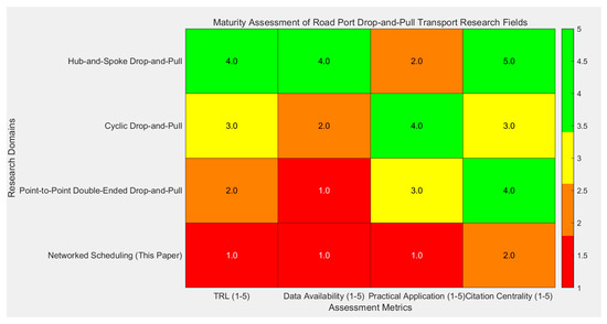
Figure 1.
Heatmap of maturity evaluation in the research field of highway port drop-and-pull transport.
As shown in Figure 1, the TRL, data availability, and centrality in the literature of the hub-and-spoke drop-and-pull system are all ≥4, indicating it is a classic high-maturity field, yet practical applications await breakthroughs. The circulating drop-and-pull system excels in practical applications, but its technical and data foundations are weak, marking it as a growing direction. The point-to-point drop-and-pull system, due to its extremely low data availability, has become a data-driven research void. Meanwhile, the comprehensive low values across all dimensions of the networked scheduling proposed in this paper confirm that this field has the lowest maturity, highlighting the necessity of the ALNS algorithm in this paper to fill the triple gaps in technology, data, and practice.
Most of the above-mentioned literature is model assumptions established from the perspectives of single car yard, single demand, and balanced demand, ignoring the actual demands of multiple car yards, multiple demands, unbalanced demands, and time windows. In terms of algorithmic solutions, the existing literature has demonstrated that the optimization problem of tractor and semitrailer transportation scheduling is classified as an NP-Hard problem [1]. Consequently, the majority of the literature employs metaheuristic and heuristic algorithms for solving this issue. However, many of these studies rely solely on theoretical parameters during local search, overlooking real-world operational contexts. Therefore, to address these limitations in existing studies, this paper develops an integrated Adaptive Large Neighborhood Search (ALNS) framework for tractor and semitrailer scheduling. The proposed approach integrates dynamic demand segmentation with time window enforcement to allocate resources according to asymmetric transport demands across highway ports, contrasting with existing hub-and-spoke or circular routing models that typically assume balanced flows. The methodology incorporates a multi-objective cost optimization model that accounts for transport costs, penalty costs, and fleet utilization, validated through a simulation of a 30-node highway port network. Experimental results demonstrate reductions of up to 61% in required tractors and 21% in operational costs, addressing key challenges in logistics operations, such as high operational expenses and low asset utilization. As illustrated in the network schematic, the critical operational parameters, including unbalanced demand volumes, service time windows, and network structure, are explicitly modeled, supporting the practical implementation. Comparative results demonstrate the superiority of the ALNS algorithm over traditional methods, providing actionable guidance for enterprise-level resource planning and scheduling.
2. Problem Description
Under network conditions, highway port tractor and semitrailer transportation enterprises possess multiple highway ports, which are distributed across different geographical locations with uneven demand. Each highway port has several tractors and ample trailer resources. Meanwhile, the customer point—referred to as highway port in this study—has relatively strict requirements for service time and usually designates a service time range, that is, the service time windows. When enterprises have scheduling tasks, they can utilize all available tractor resources within the company (including idle tractors and those in the process of performing tasks), and the number, location, demand, and time windows of highway ports are determined. The problem not only requires determining which tractor should serve each highway port but also establishing the service sequence for highway ports without violating their time window constraints. If a tractor arrives early, it can wait to serve the highway port, but the system imposes penalty costs. Due to the limited operating hours of the tractor each day, it is necessary to develop a tractor scheduling plan during this phase that minimizes network operating costs in order to increase the company’s profitability.
As shown in Figure 2, the circles represent each road port, each connected by passages between every two highway ports. A network for the tractor and semitrailer transportation business has already formed among multiple highway ports. The numbers on the lines in Figure 2 represent the tractor and semitrailer transportation volume and the required vehicle types between highway ports, while the two numbers near the highway port represent the service time windows for that highway port. For example, if the time unit is set to hours, then the service time of highway port 1 is from 7:00 to 8:00. This means that if the tractor arrives at highway port 1 between 7:00 and 8:00, the service satisfaction will be 100%. However, if it arrives before 7:00, a certain penalty cost will be incurred, leading to a decrease in service satisfaction. Additionally, arrivals after 8:00 are not permitted. After completing the task due to the constraints of working hours and the customer-service time windows, the tractor does not need to return to the starting highway port.
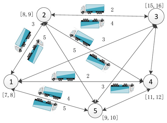
Figure 2.
Schematic diagram of optimization for tractor and semitrailer scheduling with time windows in highway ports with unbalanced demands under network conditions.
In the figure, the numbers within the circles represent the highway port numbers, and the numbers on the lines represent the tractor and semitrailer transportation volume and the required vehicle types between the formula ports. The highway port tractor and semitrailer transportation network not only exhibits the complexity of multiple car yards and diverse tractor and semitrailer demands but also possesses the following characteristics: the tractor and semitrailer demands between highway ports are often unbalanced, necessitating the segmentation of these demands and the consideration of time windows for demand matching. However, the matching relationships are unknown. Researching how to make decisions regarding the scheduling of tractors between highway ports and the configuration of the number of tractors and trailers at a lower operational cost falls under the category of more challenging NP-Hard problems.
3. Model Establishment
3.1. Model Assumptions
Based on the characteristics of tractor and semitrailer transportation in highway ports, the following assumptions are made:
(1) All tractors and semitrailers on the network are recommended models for highway tractor and semitrailer transportation; however, there are inconsistencies in the models. Furthermore, a tractor can only tow a semitrailer that does not exceed its maximum allowable towing weight. The types of tractors and semitrailers correspond to each other.
(2) The scheduling of empty semitrailers is not considered. Since the highway port also serves as a pool for semitrailers, there are sufficient semitrailers available at each highway port in the network, eliminating the need to dispatch empty semitrailers from other highway ports.
(3) The distance and time for round trips between the two highway ports are the same. This is primarily related to the operation of the tractor and semitrailer transportation vehicles. In practice, drivers use the routes recommended by Gaode Map for conducting tractor and semitrailer transportation. The assumption of uniform speed across all tractor types, regardless of load factor, is based on practical constraints: strict highway speed limits dominate the actual travel speed, making load-induced variations negligible. This simplification retains model validity while aligning with common practices in transportation research.
(4) The operation time of tractor and semitrailer is included in the driving time. This assumption is consistent with the actual tractor and semitrailer operation of the highway port, so it is reasonable.
(5) The tractor performs full-load transportation with a “one truck, one trailer” approach, meaning that the tractor can only tow one semitrailer at a time. This practice is consistent with the operational practices of highway port tractor and semitrailer transportation in China.
(6) The starting and ending points of the tractor are both located at a highway port, which may differ between the initial and terminal highway ports. Within the highway port, both the tractor and semitrailer can be parked, eliminating the need to consider the return of the tractor to the car yard after completing the transportation task. This aligns with the findings from our research on the actual operations of highway port tractor and semitrailer transportation in China.
(7) The tractor and semitrailer requirements between highway ports are independent, with no restrictions on time or transportation sequence.
(8) Every day, there is a demand for tractors and semitrailers in the network, and the demand fluctuates every day. Enterprises can schedule their operations based on the actual demand of each day, ensuring that all demands are met. Due to the long distances between some nodes, tractor and semitrailer transportation may not be completed within a single day. Therefore, it is assumed that the tractor and semitrailer tasks that were not completed the previous day do not affect the subsequent scheduling.
3.2. Symbol Explanation
The symbols applied in this paper are defined as follows:
: Collection of all highway ports, with a total of n highway ports, ;
: Number of highway ports, ;
: Collection of tractors, where ( denotes the total number of tractors);
: Index of tractor, (i.e., k represents a specific tractor in set K);
: Distance between highway ports and , in (km);
: The demand of tractor and semitrailer transportation from highway port to , expressed in terms of tractor and semitrailer transportation trips. Given that demand is not necessarily balanced, is not necessarily equal to ;
: Collection of tractor and semitrailer transportation tasks, ;
: Number of tractor and semitrailer transportation tasks, . Also, a and b represent specific tasks designated for empty-load trips, where a denotes origin and b denotes destination).
, : Cost of heavy semitrailer and empty driving of tractor, in (CNY/km);
: Fixed cost of tractor per unit time, including vehicle depreciation, employee salary, etc., in (CNY);
: Penalty cost incurred by the early arrival of the tractor within a unit of time, in (CNY/h);
: Continuous working hours of tractor, all of which are stipulated to have equal continuous working hours each day;
: Speed of tractor when towing heavy semitrailer and empty driving, in (km/h);
: The time windows of each task, where represents the lower limit of the time window of the s-th tractor and semitrailer task, and represents the upper limit of the time window of the s-th tractor and semitrailer task;
: A sufficiently large positive constant. It is used to enforce sequential uniqueness of tasks in constraint (6) by penalizing invalid assignments.
Decision variable:
, : The number of times that tractor drives from highway port to with heavy semitrailer and empty driving;
: The sequence in which tractor services task ;
: The time when the tractor reaches the transportation starting point of -item tractor and semitrailer task;
: The total number of tractors required by the highway network;
is a piecewise linear function. When (the time when the tractor arrives the start point of the tractor and semitrailer task is earlier than the lower limit of the time window of this task), the value is , and the value of is . When (the tractor arrives between the lower and upper limits of the time window for the tractor and semitrailer task), the value is 0.
3.3. Mathematical Model
According to the actual operation of tractor and semitrailer transportation in highway ports under the condition of networked operation, tractor and semitrailer transportation enterprises pursue the minimum operation cost of the highway port network.
(1) Objective function
The cost of network operation consists of the cost of heavy semitrailer driving, empty driving, and fixed costs. The cost of heavy semitrailer driving is ; the cost of empty driving is ; the fixed cost of using the vehicle on that day is ; and the cost of penalty is . The goal of minimizing the network operation cost is expressed as follows:
(2) Constraint conditions
To ensure the feasibility and effectiveness of the proposed optimization model, the following constraints are formulated. These constraints define the relationships among tractors, semitrailer tasks, scheduling sequences, routing conditions, and time windows.
First, each tractor–semitrailer task must be uniquely assigned to one tractor, ensuring that all transport demands are fulfilled without redundancy. The corresponding constraint is as follows:
Next, the total number of heavy-load trips must precisely satisfy the transport demand between highway ports, and it is enforced by the constraint shown below:
To prevent idle resources from being counted, a tractor is only activated when it is assigned to at least one task, as expressed by the following constraint:
Additionally, when a tractor is not assigned to a task, its service sequence number must be zero, as shown below:
To guarantee correct task execution order, any two tasks served by the same tractor must be assigned different sequence numbers. The constraint ensuring this is as follows:
Moreover, the service sequence number for each task must lie within a valid range, which is formulated as follows:
The number of heavy-load trips for each tractor is derived from its assigned task routes, as captured by the following constraint:
In parallel, the number of empty-load trips is determined by transitions between consecutive tasks:
To support fleet planning, the total number of tractors used is tracked via the following expression:
Routing indicators are then defined to identify whether each tractor travels along a specific port route in either loaded or empty condition, as expressed as follows, respectively:
To avoid logical errors in the transport plan, each task must involve different origin and destination ports, enforced by the following:
From an operational perspective, the total working time for each tractor must not exceed a predefined maximum, ensuring regulatory compliance and driver safety. The constraint is shown below:
Finally, to meet service-level requirements, each task must be completed within its allocated time window, as represented by the following:
4. Design of ALNS Algorithm
The optimization of the scheduling of demand-uneven highway ports with time windows under network conditions is classified as an NP-Hard problem [2], making it challenging to obtain satisfactory solutions within a short timeframe. The ALNS algorithm is a metaheuristic well-suited for solving complex scheduling problems due to its adaptability and solution quality. It can self-adaptively adjust its search strategies based on the characteristics of the problem and the quality of the solutions, making it effective in solving complex combinatorial optimization problems. Accordingly, the proposed solution utilizes the ALNS algorithm, where each transportation between two highway ports is modeled as a task unit. Through iterative destruction and repair operations on these units, the algorithm continuously generates and refines feasible scheduling solutions. The destroy operator is designed with three types: random destruction, correlation destruction, and complete vehicle removal. Similarly, the repair operator is also designed with three types, namely target optimal greedy insertion, empty load minimum greedy insertion, and waiting time minimum greedy insertion. By combining adaptive adjustment of the destroy ratio and introducing a simulated annealing mechanism for accepting new solutions, the search capability of the ALNS algorithm is enhanced. The algorithm flowchart is shown in Figure 3, and the detailed steps are given as follows.
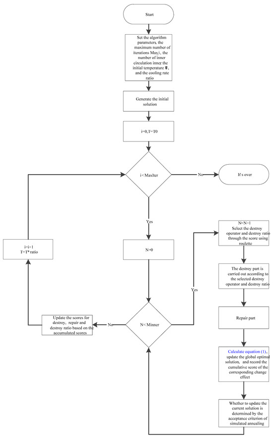
Figure 3.
Algorithm flowchart.
4.1. Step 1: Parameter Initialization
The algorithm begins with the initialization of key parameters. The input parameters include the following:
: The number of inner iterations per outer loop, controlling the local search intensity;
: The maximum number of outer loop iterations, serving as the termination condition;
: The initial temperature in the simulated annealing framework, which influences the acceptance probability of inferior solutions;
: The cooling rate that determines the temperature-update schedule.
Additionally, the initial scores assigned to the destroy and repair operators are uniformly set to equal values. Similarly, the initial scores for the candidate set of destroy ratios are initialized equally to ensure a balanced starting point for adaptive selection during the search process.
4.2. Step 2: Initial Solution Generation
The second step is initial solution generation. The feasible initial solution, , is generated by using the construction method of the initial solution designed in the previous text. The global optimal solution, , is initialized; the outer-circulation counter, , is set; and the temperature initialization, , is carried out. During the initial solution construction, a transportation task between two highway ports is considered as a unit, and a target-optimal greedy insertion approach is employed to generate a set of tractor routes.
4.3. Step 3: Inner-Circulation Initialization
In this step, the inner iteration counter is reset by setting .
4.4. Step 4: Neighborhood Search Operation
In this step, the inner iteration counter is updated as . A destroy operator is selected using a roulette-wheel selection mechanism, guided by the adaptive scores assigned to each operator and the corresponding destruction ratio. The destroy phase comprises three components: a random destruction operator, a correlation-based destruction operator, and a full-truck destruction operator. In the repair phase, the empty-load minimization greedy insertion and waiting-time minimization greedy insertion are adopted for processing. Once selected, the destroy and repair operations are applied sequentially to the current solution, , thereby generating a new candidate solution.
The new solution of Equation (1) is then evaluated. If the new solution yields a better performance than the current global best, the global optimal solution, , is accordingly updated.
4.5. Step 5: Solution-Update Strategy
If the target value of the new solution is better than that of the current solution, the current solution will be replaced by the new solution. Otherwise, the acceptance criterion of simulated annealing will be used to determine whether to update the current solution. Based on the solution’s status (better than global optimum/better than current/worse than current/not selected), the corresponding score increment will be temporarily stored.
4.6. Step 6: Inner-Circulation Control
After each iteration of the inner circulation, a termination check is performed. If the number of inner iterations, , has not reached the predefined maximum, , the algorithm returns to Step 4 to continue the local search process at the current temperature level.
Once , the local search at the current temperature is considered complete. The algorithm then proceeds to the outer loop-update phase, where the temperature is adjusted and operator scores are updated based on the accumulated feedback from this inner circulation.
4.7. Step 7: Outer-Circulation Update
At the end of the inner loop, the outer iteration counter is incremented as , and the temperature is updated according to the cooling schedule: .
Subsequently, based on the performance outcomes observed during the inner iterations, the scores of the selected destroy operator, repair operator, and destroy ratio are updated accordingly. This adaptive mechanism helps guide the operator selection in future iterations by reinforcing strategies that contribute to improved solutions.
4.8. Step 8: Termination Determination
The algorithm checks whether the outer iteration limit has been reached. If , the algorithm returns to Step 3 to begin the next outer iteration cycle. Otherwise, the process proceeds to Step 9, concluding the optimization procedure.
4.9. Step 9: Result Output
Upon completion of all outer iterations, the algorithm terminates and returns the global optimal solution, , obtained during the search process.
5. Simulation
The following simulation example is conducted to validate and demonstrate the applicability of the proposed method.
Relying on the highway port tractor and semitrailer transportation network, tractor and semitrailer transportation companies have established highway ports in 30 cities. A technical issue that managers wish to address is how to arrange vehicle scheduling within the highway port network to minimize the overall operational costs of the entire network. Assuming the cost of the tractor with heavy and empty hanging driving, represented by , , and the speed of the heavy and empty hanging driving is represented by . The fixed daily cost is , and the continuous working time per day is . The waiting cost is denoted as . The value of is determined based on the route recommended by Gaode Map. The values are generated using the randint function in MATLAB 2010a, producing 30 tractor and semitrailer transportation tasks between highway ports within the range of [0, 10]. In ALNS, the population size is set to 10, and the number of iterations is 10. For the simulated annealing parameters, the initial temperature is set to 100, and the cooling rate is 0.95. Each tractor and semitrailer transportation task is solved via integer programming, and the algorithm runs 30 times to select the optimal solution as the final result.
5.1. Result Analysis Under Fixed Working Hours
Through calculations, it is determined that 1666 tractors are required to complete the designated tasks, with the number of each tractor listed in Table 3. As shown in Table 4, compared to traditional transportation methods, the number of tractors has decreased by 9%, resulting in a cost savings of 3%. The tractor-to-semitrailer ratio is 1.00:1.10, which reflects the superiority of network-based tractor and semitrailer.
Table 3.
Operation results of tractor and semitrailer scheduling with time windows in highway ports with unbalanced demand under network conditions.
Table 4.
Comparison of calculation results between traditional transportation methods and network-based tractor and semitrailer transportation.
5.2. Comparison of Results Under Different Working Hours
As the working hours of the tractors increase, the advantages of long-haul transportation through tractor and semitrailer transportation will be maximized, leading to an increase in the number of highway ports served, thereby resulting in various scheduling schemes for tractors. To this end, the working hours of the tractor in the calculation example will be extended to 16, 32, 48, and 72 h, respectively. The specific calculation results are shown in Table 5.
Table 5.
Comparison of results under different working hours of tractors.
The results indicate a close relationship between the number of tractors used, the total costs, the tractor-to-semitrailer ratio, and the working hours of the tractors. Specifically, (1) compared to China’s tractor-to-semitrailer ratio of 1.00:1.04 in 2024, the ratios in the calculation example are all higher than this value and are directly proportional to the working hours of the tractors. The higher tractor-to-semitrailer ratio indicates that each tractor can pull a greater number of semitrailers along its route, resulting in better utilization of tractors within the transportation network, higher vehicle configuration efficiency, and lower operational costs of the network. This demonstrates the advantages of network-based tractors and semitrailers. (2) The longer the working hours of the tractor, the fewer the number of tractors used, the lower the total cost, and the higher tractor-to-semitrailer ratio. (3) As the working hours of the tractor increases, both the reduction ratio of the number of tractors and the total cost savings exhibit a trend of gradual increase. This trend is particularly pronounced when the working hours of the tractor reaches 72 h, highlighting the advantages of network-based tractor and semitrailer. (4) The determination of the reasonable values for the tractor-to-semitrailer ratio under different working hours also provides decision-making support for highway port tractor and semitrailer transportation enterprises in the procurement of tractors and semitrailers.
5.3. Comparison of Results Under Different Algorithms
To further validate the performance of the algorithm, this paper will compare the improved Ant Colony Algorithm (IACS) with the ALNS algorithm. In the IACS algorithm, is the maximum number of iterations, set to 600; is the parameter representing the importance of pheromone, set to 1; and is the parameter representing the importance of the heuristic factor, set to 4. To ensure statistical reliability, each algorithm was independently run 30 times, with the final results computed as the mean of all executions. The results are compared in Table 6.
Table 6.
Comparison of algorithm results under different working hours of tractors.
As shown in Table 6, the data for the tractors using the ALNS algorithm and the total cost are both lower than those of the IACS algorithm. Therefore, considering all factors, it is concluded that the ALNS algorithm is superior, and its advantages in finding optimal solutions when dealing with large-scale problems have been demonstrated.
5.4. Verification of Algorithm Robustness
In this section, the effectiveness of the proposed ALNS is evaluated by setting different values for the hyperparameters. The algorithm is implemented in MATLAB, and the experimental operating environment is a 64-bit Windows 11 operating system, with an Intel® CoreTM i5-8265U CPU @ 1.60GHz 1.80 GHz processor and 8 GB of RAM.
To clarify the robustness of the ALNS algorithm against hyperparameter fluctuations and to support its engineering practicality, this study focuses on three core control dimensions of the ALNS algorithm: local search intensity, global exploration capability, and simulated annealing mechanism. It sets multiple typical values for four types of hyperparameters, covering the effective range verified by preliminary experiments. Combined with four tractor working durations, a total of 324 full factorial sensitivity experiments are conducted. The experimental results are quantitatively presented in Table 7.
Table 7.
Summary of parameter sensitivity analysis.
As can be seen from the Table 7, when the algorithm hyperparameters vary within a reasonable range (e.g., the number of inner loops ∈ {5, 10, 15}), the total cost fluctuation range is ≤1.2%, and the coefficient of variation is ≤1.5%, which is significantly lower than the impact range of the tractor working duration of 17–18%. This indicates that minor adjustments to the hyperparameters have an extremely weak effect on the results, the dispersion degree of the results is extremely low, and the algorithm exhibits strong robustness. The reduction in total cost attributed to the working hours of tractors is 17–18%, significantly greater than the optimization contribution of hyperparameters (≤1.2%). This demonstrates that the superiority of the algorithm stems from its alignment with the essence of issues such as “long-haul drop and hook transportation,” rather than relying on meticulous hyperparameter tuning.
In summary, this experiment quantitatively proves that the optimization effectiveness of the ALNS algorithm exhibits strong robustness against hyperparameter fluctuations, and its superiority does not depend on a narrow parameter-tuning range. The engineering value of this conclusion indicates that, in practical highway port scheduling, parameters are difficult to calibrate precisely, and the low sensitivity of ALNS ensures the algorithm’s practicality in complex scenarios.
6. Conclusions
Compared to traditional transportation, network-based tractor and semitrailer transportation has lower operational costs, indicating that it can arrange transportation capacity more appropriately and make full use of resources. As the working hours of the tractors increase, network-based tractor and semitrailer transportation can improve the tractor-to-semitrailer ratio, reduce the empty-load rate and empty distance of the tractors, enhance the utilization efficiency of the tractors, and optimize vehicle configuration, thereby lowering network operational costs. This also demonstrates the effectiveness of the ALNS algorithm. Future research will incorporate case studies on tractor and semitrailer transportation in different regions and dynamic actual demand data to provide more refined guidance for highway port tractor and semitrailer transportation enterprises.
Author Contributions
Conceptualization, H.G. and Y.H.; methodology, H.G. and Y.H.; software, H.G., Y.H., and F.W.; formal analysis, H.G.; resources, H.G. and Y.H.; writing—original H.G.; preparation, H.G.; writing—review and editing, H.G., Y.H., and F.W.; visualization, H.G.; supervision, H.G. and Y.H.; project administration, H.G. and Y.H.; correspondence and final manuscript review, Y.Z.; funding acquisition, H.G. and Y.H. All authors have read and agreed to the published version of the manuscript.
Funding
This research was funded by Guangxi University of Science and Technology Doctoral Fund Project, grant number 24Z02; Specific Research Project of Guangxi for Research Bases and Talents, grant number AD23026317; Guangxi University of Science and Technology Doctoral Fund Project, grant number 20S08.
Data Availability Statement
The original contributions presented in this study are included in the article/supplementary material. Further inquiries can be directed to the corresponding author(s).
Conflicts of Interest
The authors declare no conflicts of interest.
Abbreviations
| ALNS | Adaptive Large Neighborhood Search |
| IACS | Improved Ant Colony System |
| TSRP | Tractor and Semitrailer Routing Problem |
| TRL | Technology Readiness Level |
References
- Li, H.Q.; Lv, T. A review of research on car and train scheduling problems. J. Dalian Marit. Univ. 2015, 14, 1–10. [Google Scholar]
- Nomikos, N.K.; Tsouknidis, D.A. Disentangling demand and supply shocks in the shipping freight market: Their impact on shipping investments. Marit. Policy Manag. 2023, 50, 563–581. [Google Scholar] [CrossRef]
- Tian, R.L.; Meng, Q.W. Research on the Scheduling of Container Semitrailers Matched with Heavy Equipment Tractors. Eng. Technol. Natl. Def. Transp. 2017, 15, 18–21+37. [Google Scholar] [CrossRef]
- Li, H.; Chang, X.; Zhao, W.; Lu, Y. The vehicle flow formulation and savings-based algorithm for the rollon-rolloff vehicle routing problem. Eur. J. Oper. Res. 2017, 40, 867–872. [Google Scholar] [CrossRef]
- Li, H.; Jian, X.; Chang, X.; Lu, Y. The generalized rollon-rolloff vehicle routing problem and savings-based algorithm. Transp. Res. Part B Methodol. 2018, 113, 1–23. [Google Scholar] [CrossRef]
- Yang, Z.H.; Wang, Z.C.; Wei, Z.K.; Jin, Z.H. Dynamic Tractor-and-semitrailer routing problem with the non-deterministic operation time of trailers. Syst. Eng.-Theory Pract. 2021, 41, 1081–1095. [Google Scholar]
- Peng, Y.; Gao, H. Path optimization of multi-trip swap-body vehicle routing problem with time window. J. Transp. Syst. Eng. Inf. Technol. 2020, 2, 166–174. [Google Scholar] [CrossRef]
- Li, H.; Lv, T.; Li, Y. The tractor and semitrailer routing problem with many-to-many demand considering carbon dioxide emissions. Transp. Res. Part D Transp. Environ. 2015, 34, 68–82. [Google Scholar] [CrossRef]
- Li, H.Q.; Chang, X.Y.; Zhu, X.N.; Lu, Y. Intercity Line-haul Tractor Dispatching Problem in Trailer Pick-up Transport and Its Solving Method. J. Highw. Transp. Res. Dev. 2016, 33, 151–157. [Google Scholar]
- Regnier, C.O.; Mccall, J.; Ayodele, M.; Anderson, S. Truck and trailer scheduling in a real world dynamic and heterogeneous context. Transp. Res. Part E Logist. Transp. Rev. 2016, 93, 389–408. [Google Scholar] [CrossRef]
- Jin, Z.H.; Yan, H.; Wang, X.H.; Xing, L.; Xu, Q. Scheduling Optimization and Operation Mode Analysis on Ro-ro Tractor-and-trailer Transportation. J. Transp. Syst. Eng. Inf. Technol. 2022, 22, 142–151. [Google Scholar] [CrossRef]
- Yu, L.; Lin, H.; Chen, B.R. Research of vehicle scheduling problem of the network drop and pull transport. J. Transp. Eng. Inf. 2014, 12, 58–64. [Google Scholar]
- Wang, Q.B.; Yu, J.N.; Zheng, J.F. Interference Management Model for Drop and Pull Transport with New Tasks. J. Transp. Eng. Inf. 2021, 21, 160–166+225. [Google Scholar] [CrossRef]
- Zhou, Y.S.; Ni, S.Q.; Chen, D.J.; Wang, W.X. Simulation of Vehicle Quantity Optimization of Tractor and Trailer in Drop and Pull Transport. Comput. Simul. 2024, 41, 121–132. [Google Scholar]
- Subramanian, A.; Penna, P.H.V.; Uchoa, E.; Ochi, L.S. A hybrid algorithm for the Heterogeneous Fleet Vehicle Routing Problem. Eur. J. Oper. Res. 2012, 221, 285–295. [Google Scholar] [CrossRef]
- Villegas, J.G.; Prins, C.; Prodhon, C.; Medaglia, A.L.; Velasco, N. A matheuristic for the truck and trailer routing problem. Eur. J. Oper. Res. 2013, 230, 231–244. [Google Scholar] [CrossRef]
- Tütüncü, G.Y. An interactive GRAMPS algorithm for the heterogeneous fixed fleet vehicle routing problem with and without backhauls. Eur. J. Oper. Res. 2009, 201, 593–600. [Google Scholar] [CrossRef]
- Oliviu, M.; Jozsef, L.S.; Camelia, C.; Pop, P.C. An improved immigration memetic algorithm for solving the heterogeneous fixed fleet vehicle routing problem. Neurocomputing 2015, 150, 58–66. [Google Scholar] [CrossRef]
- Li, H.; Wang, H.; Chen, J.; Bai, M. Two-echelon Vehicle Routing Problem with Time Windows and Mobile Satellites. Transp. Res. Part B Methodol. 2020, 138, 179–201. [Google Scholar] [CrossRef]
- Farid, G.S.; Abdolhadi, Z. Multi-objective heterogeneous vehicle routing and scheduling problem with energy minimizing. Swarm Evol. Comput. 2018, 44, 728–747. [Google Scholar] [CrossRef]
- Bevilaqua, A.; Bevilaqua, D.; Yamanaka, K. Parallel island based Mimetic Algorithm with Lin–Kernighan local search for a real-life Two-Echelon Heterogeneous Vehicle Routing Problem based on Brazilian wholesale companies. Appl. Soft Comput. 2019, 76, 697–711. [Google Scholar] [CrossRef]
- Srivastava, G.; Singh, A.; Mallipeddi, R. NSGA-II with objective-specific variation operators for multi objective vehicle routing problem with time windows. Expert Syst. Appl. 2021, 176, 114779. [Google Scholar] [CrossRef]
- Soares, R.; Marques, A.; Amorim, P.; Rasinmäki, J. Multiple vehicle synchronization in a full truck-load pickup and delivery problem: A case-study in the biomass supply chain. Eur. J. Oper. Res. 2019, 277, 174–194. [Google Scholar] [CrossRef]


Disclaimer/Publisher’s Note: The statements, opinions and data contained in all publications are solely those of the individual author(s) and contributor(s) and not of MDPI and/or the editor(s). MDPI and/or the editor(s) disclaim responsibility for any injury to people or property resulting from any ideas, methods, instructions or products referred to in the content. |
© 2025 by the authors. Licensee MDPI, Basel, Switzerland. This article is an open access article distributed under the terms and conditions of the Creative Commons Attribution (CC BY) license (https://creativecommons.org/licenses/by/4.0/).