A Special Family of Triangles

Abstract

We study the one-parameter family of triangles that emerges if one sideline traces a pencil of lines and the opposite angle is fixed. A description of the traces of triangle centers and the pair of Brocard points in terms of parametrizations and equations is given. The envelopes of the families of circumcircles and nine-point circles are determined. Our approach even allows us to consider and treat the triangle family as a two-parameter family of triangles; i.e., the (interior) angle opposite to the pencil, which is in the beginning fixed, may also change.

1. Introduction

1.1. Related and Prior Work

Triangle geometry is rich with elegant results and deep relations between points, lines, angles, circles, and related curves. The study of triangles and their families even nowadays attracts many geometers. Some results in this area, especially for the Euclidean plane, can be found in [1,2,3,4,5,6] while [7,8,9] deal with the situation in the isotropic plane.

1.2. Contributions and Aims of the Present Paper

We intend to approach some results of this particular family of triangles in an analytical way. This is because of the following two reasons: 1. A synthetic approach is already given in [6]. There is no reason to repeat this, and nothing can be added. 2. The synthetic approach is limited, though very elegant, and gives some geometric insight into the problem. We shall omit the discussion of traces and loci of midpoints of changing segments, envelopes of bisectors of angles, and segments and all other objects that are not “central” in the sense of [10,11]. There is only one exception: In Section 3.2, we shall have a look at the bicentric pair of Brocard points. They are closely related to some important triangle centers. Further, we determine and discuss the envelopes of special central circles. The envelope of the Euler line appears to be rather unspectacular and is, therefore, not discussed. The envelopes of circles can be determined much easier in a suitable analytic approach than with the synthetic approach.

In Section 2, we shall build the analytical environment, i.e., we introduce coordinates in a way that we are able to move through the computations in the present paper. This allows us to parametrize the triangle family under consideration, and further, enables us to give the first results. In particular, we can show that all centers (and points) on the Euler line forming a fixed affine ratio with the centroid and the circumcenter move on hyperbola. In Section 3, the envelopes of the families of circumcircles and and nine-point circles are determined. Then, we move over to the Brocard points and some triangle centers related to them. Finally, Section 4, we shall give the equations of the traces some more triangle centers. As can be expected, some triangle centers run on quartic curves, some on curves of much higher degree. This seems to depend on the algebraic complexity of the construction of the respective centers. Section 5 poses open questions and gives hints towards future work.

2. Analytical Framework

We assume that the vertex A of the triangle $\Delta =ABC$ coincides with the origin of a Cartesian coordinate system. The line $[A,B]$ shall be the x-axis of the frame and the line $[C,A]$ (which encloses the angle $0<\alpha <\pi$ with the x-axis) is given by the equation $xsin\alpha -ycos\alpha =0$ as indicated in Figure 1 (left).

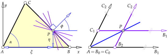
Figure 1. Geometric meaning of parameters (left), degenerate triangles in the pencil (right).

The pencil of lines carrying the third side of $\Delta$ shall be centered at $P=(\xi ,\eta )$ with $\eta \ne 0$ (i.e., $P\notin [A,B]$) and $\xi sin\alpha -\eta cos\alpha \ne 0$ (i.e., $P\notin [C,A]$).

Now, we assume that $\varphi \in \mathbb{R}$ is a coordinate in the pencil of lines about P and $(cos\varphi ,sin\varphi )\in {\mathrm{S}}^1$ is a unit normal vector of the side line $[B,C]\ni P$. Hence, an equation of $[B,C]$ is given by $xcos\varphi +ysin\varphi =d$, where $d:=\xi cos\varphi +\eta sin\varphi$ is the support function of $[B,C]$.

The remaining vertices of the triangle $\Delta$ are then found as the intersection of $[B,C]$ with $[A,B]$ and $[C,A]$. So, the three vertices of $\Delta$ are parametrized by the following:

$$A=(0,0),B={\displaystyle \frac{d}{cos\varphi }}\left(1,0\right),C={\displaystyle \frac{d}{cos(\alpha -\varphi )}}\left(cos\alpha ,sin\alpha \right).$$

(1)

This describes a one-parameter family $\mathcal{T}$ of triangles. Allowing further $\alpha$ to trace ${\mathrm{S}}^1$, we have parametrized a two-parameter family of triangles.

In principle, the parameter $\varphi$ is allowed to trace ${\mathrm{S}}^1$ freely. However, $\varphi ={\displaystyle \frac{\pi }{2}},{\displaystyle \frac{3\pi }{2}}$ results in an open triangle $A{B}_1{C}_1$ (cf. Figure 1, right), the vertex $B_1$ is at infinity, and $[B,C]$ is either anti-parallel to $[A,B]$ (if $\varphi ={\displaystyle \frac{\pi }{2}}$) or parallel to $[A,B]$ (if $\varphi ={\displaystyle \frac{3}{2}}\pi$). If $\varphi =arctan{\displaystyle \frac{\eta }{\xi }},arctan{\displaystyle \frac{\eta }{\xi }}+\pi$, the line carrying $[B_0,C_0]$ passes through A and the corresponding two triangles ${\Delta }_0=A{B}_0{C}_0$ are point-shaped (see also Figure 1). Finally, if $\varphi =\alpha +{\displaystyle \frac{\pi }{2}},\alpha +{\displaystyle \frac{3\pi }{2}}$, we obtain the second pair of open triangles $A{B}_2{C}_2$ (cf. Figure 1).

All loci of points (and especially centers) related to the triangles in the family $\mathcal{T}$ are traced twice, since $\Delta \left(\varphi \right)=AB\left(\varphi \right)C\left(\varphi \right)=\Delta (\varphi +\pi )=AB(\varphi +\pi )C(\varphi +\pi )$ agree as congruent triangles with differently oriented side line $[B,C]$.

Now, the analytical representation (1) allows us to formulate the following:

Theorem 1.

The centroid $X_2$, the circumcenter $X_3$, and the orthocenter $X_4$ of Δ run on hyperbolae, while $[B,C]$ traverses the pencil about P.

Proof. 

A parametrization of the centroid $X_2$ in terms of the underlying Cartesian coordinates is obtained as the arithmetic mean of the coordinate vectors (1) of $\Delta$’s vertices. This yields the following

$$X_2\left(\varphi \right)={\displaystyle \frac{d}{3cos\varphi cos(\alpha -\varphi )}}\left(2cos\alpha cos\varphi +sin\alpha sin\varphi ,sin\alpha cos\varphi \right)$$

(2)

which, after implicitization, i.e., after the elimination of the parameter $\varphi$ results in the implicit equation

$${\mathcal{H}}_2:3xysin\alpha -3y^{2}cos\alpha +(2\eta cos\alpha -\xi sin\alpha )y-x\eta sin\alpha =0.$$

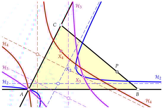
The latter is the equation of a hyperbola with asymptotes $xsin\alpha -ycos\alpha =0$ and $y=0$ (since $\alpha \ne 0$), i.e., one is parallel to $[A,B]$, the other one is parallel to $[C,A]$, cf. Figure 2.

Figure 2. The hyperbolae ${\mathcal{H}}_2$ (blue), ${\mathcal{H}}_3$ (magenta), ${\mathcal{H}}_4$ (red) as the orbits of the centroid $X_2$, the circumcenter $X_3$, and the orthocenter $X_4$ of the triangles in the pencil of triangles.

The circumcenter $X_3$ is the intersection of the bisectors of $\Delta$’s sides. We obtain the parametrization

$$X_3\left(\varphi \right)={\displaystyle \frac{d}{2cos\varphi }}\left(1,{\displaystyle \frac{sin(\alpha -\varphi )}{cos(\alpha -\varphi )}}\right),$$

(3)

and further, by eliminating $\varphi$, the implicit equation

$${\mathcal{H}}_3:2x^{2}cos\alpha +2xysin\alpha -(\xi cos\alpha +\eta sin\alpha )x-(\xi sin\alpha -\eta cos\alpha )y=0.$$

It is rather elementary to verify that the latter is the equation of a hyperbola. The equations of its asmptotes are the linear factors of the quadratic form, see [12]. This makes clear that ${\mathcal{H}}_3$ passes through the ideal points of the lines orthogonal to $[A,B]$ and $[C,A]$. ${\mathcal{H}}_3$ is centered at

$${\displaystyle \frac{1}{2{sin}^2\alpha }}\left(sin\alpha (\xi sin\alpha -\eta cos\alpha ),\eta (1+{cos}^2\alpha )-\xi cos\alpha sin\alpha \right).$$

(4)

In order to complete the proof, we determine the orthocenter $X_4$ of $\Delta$ and find the parametrization

$$X_4\left(\varphi \right)={\displaystyle \frac{dcos\alpha }{cos\varphi cos(\alpha -\varphi )}}\left(cos\varphi ,sin\varphi \right),$$

that annihilates the following equation

$${\mathcal{H}}_4:x^{2}cos\alpha +xysin\alpha -\eta ycos\alpha -\xi xcos\alpha =0.$$

Which clearly describes a hyperbola centered at

$$\left(\eta {\displaystyle \frac{cos\alpha }{sin\alpha }},\xi {\displaystyle \frac{cos\alpha }{sin\alpha }}-\eta {\displaystyle \frac{{cos}^2\alpha }{{sin}^2\alpha }}\right),$$

(5)

and passing through the ideal points of the normals to the fixed side lines of the triangles in the family. □

We shall also note that the centers (4) of the hyperbola housing the circumcenters of the triangles in the family trace the parabola

$$8x^2-6\xi x-2y\eta +{\xi }^2+{\eta }^2=0$$

if the triangles’ interior angle $\alpha$ traces ${\mathrm{S}}^1$. The centers (5) of the hyperbola generated by the orthocenters run on the parabola

$$2x^2-\xi x+\eta y=0.$$

The existence of a parabola as loci of centers of the hyperbolic orbits fit well with a much larger concept. So far, we have considered the orbits of three centers which are collinear, i.e., they lie on the Euler line. In this respect, we can show the following result:

Theorem 2.

Any but two points X on the Euler line moves on a hyperbola while the moving triangle side traverses its pencil. The exceptional points move on the interior and exterior angle bisector through A and deliver the only degenerate conical loci of points on the Euler line. The centers of the hyperbola move on a parabola if the angle α at A traverses ${\mathrm{S}}^1$.

Proof. 

The parametrizations (2) and (3) of the orbits of $X_2$ and $X_3$ can be used to parametrize the range of points on the Euler line ${\mathcal{L}}_{2,3}$ and we have

$${\mathcal{L}}_{2,3}\left(w\right)=X_2(1-w)+X_{3}w,w\in \mathbb{R}.$$

(6)

We eliminate the parameter $\varphi$ in the pencil of lines about P. For the sake of simplicity, we replace the trigonometric functions of $\alpha$ by their rational equivalents

$$cos\alpha ={\displaystyle \frac{1-a^2}{1+a^2}},sin\alpha ={\displaystyle \frac{2a}{1+a^2}}.$$

Then, we find the quadratic equation of the orbits of the points ${\mathcal{L}}_{2,3}\left(w\right)$

$$\begin{array}{c}6\left((w(3a^4-2a^2+3)+8a^2)x+(4aw(1-a^2)+4a(a^2-1))y\right)\left(3(a^2-1)wx-2a(w+2)y\right)\\ +(w(3a^2-1)+4)(w(a^2-3)-4a^2)(3w(a^2-1)\xi -2a(w+2)\eta )x\\ -(2a(w+2)\xi +(w(1-a^2)+4(a^2-1))\eta )y)=0.\end{array}$$

The latter is the equation of a hyperbola, since it shares the ideal points with the lines

$$\begin{array}{c}(w(3a^4-2a^2+3)+8a^2)x+(4wa(1-a^2)+4a(a^2-1))y=0,\\ 3w(a^2-1)x-2a(w+2)y=0.\end{array}$$

The hyperbola degenerates if the following is met

$$w\in \left\{{\displaystyle \frac{4}{1-3a^2}},{\displaystyle \frac{4a^2}{a^2-3}}\right\}$$

and becomes either the repeated line $ay+x=0$ or the repeated line $ax-y=0$. Since $a=tan{\displaystyle \frac{\alpha }{2}}$, these repeated lines are the interior and exterior angle bisector of $\Delta$ at A.

The centers of the hyperbola depending on the angle $\alpha$ can be described as

$${\displaystyle \frac{1}{12a^2}}\left(a(w(3a^2\eta +2a\xi -3\eta )+4a\xi ),w(3a(a^2-1)\xi +(3a^4-4a^2+3)\eta )+4a^2\eta \right),$$

which clearly shows that for a fixed angle $\alpha$ (a family of triangles with a common angle at A), the centers of the orbits of points ${\mathcal{L}}_{2,3}\left(w\right)$ trace a straight line. However, we aim at the description of the locus of the orbits of the centers for varying $\alpha$. For that purpose, we eliminate $\alpha$ (or a) and obtain the equation

$$72x^2-6\xi (w+8)x-18w\eta y+3w^2{\eta }^2-w^2{\xi }^2+6w{\eta }^2+2w{\xi }^2+8{\xi }^2=0$$

of parabola that touch the ideal line in the ideal point of y-axis. □

3. Some Envelopes

3.1. The One-Parameter Family of Circumcircles

With (3) we have already found an analytic representation of the circumcenters of the triangles in the family $\mathcal{T}$. An equation of the one-parameter family of circumcircles of the triangles in $\mathcal{T}$ can be obtained, since the radius function equals $R=\overline{X_{3}A}$. The circumcircles of the triangles in the family $\mathcal{T}$ have the equation(s)

$$\mathcal{U}:cos\varphi cos(\alpha -\varphi )(x^2+y^2)-dcos(\alpha -\varphi )x-dsin(\alpha -\varphi )x=0,$$

(7)

where $d=d\left(\varphi \right)$ is the support function of the line $[B,C]$ which still depends on $\varphi$ (a fact that should be taken into account when it comes to the computation of the envelope).

The envelope of the circles (7) is now found by first differentiating $\mathcal{U}$ with respect to $\varphi$ and the subsequent elimination of $\varphi$ from both $\mathcal{U}$ and $\partial \mathcal{U}/\partial \varphi$. The elimination is simplified by replacing $cos\varphi$ and $sin\varphi$ by their rational equivalents. Besides some constant factors, the resultant of $\mathcal{U}$ and $\partial \mathcal{U}/\partial \varphi$ contains the factors

$${(x^2+y^2)}^2,{({(x-\xi )}^2+{(y-\eta )}^2)}^2,$$

which can be canceled, for they describe pairs of isotropic lines (of Euclidean Geometry, cf. [12] p. 253). Any isotropic line splits off with multiplicity two from the envelope.

The essential part of the resultant yields the equation

$$\begin{array}{c}{\mathcal{E}}_{\mathcal{U}}:{sin}^2\alpha {(x^2+y^2)}^2\\ -2(x^2+y^2)\left(sin\alpha (\xi sin\alpha -\eta cos\alpha )x+(\eta (1+{cos}^2\alpha )-\xi sin\alpha cos\alpha )y\right)\\ +{\left((\eta cos\alpha -\xi sin\alpha )x+(\xi cos\alpha +\eta sin\alpha )y\right)}^2=0.\end{array}$$

(8)

We can summarize the results as follows:

Theorem 3.

The envelope of the circumcircles of all triangles in the one-parameter triangle family $\mathcal{T}$ is a rational and bicircular quartic curve ${\mathcal{E}}_{\mathcal{U}}$ with ordinary double points at the absolute points of Euclidean geometry and a cusp of the second kind at the point A. The tangent to the super-linear branch at A is given by the equation

$$(\eta cos\alpha -\xi sin\alpha )x+(\xi cos\alpha +\eta sin\alpha )y=0$$

and encloses the angle $|\alpha -\psi |$ with the line $[A,P]$, where $\psi =\angle PAB$.

Figure 3 shows the quartic curve ${\mathcal{E}}_{\mathcal{U}}$ for a specific choice of $\alpha$.

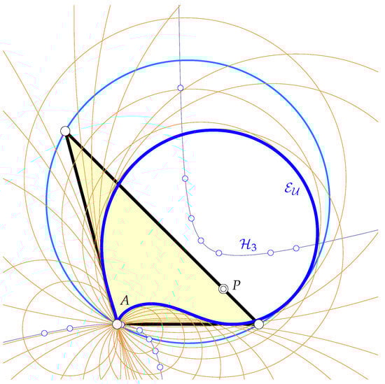
Figure 3. The envelope ${\mathcal{E}}_{\mathcal{U}}$ of the one-parameter family of circumcircles always has a cusp at A.

The computation of the nine-point circles as the circumcircles of the medial triangles of the totality of triangles in $\mathcal{T}$ is nearby. Their equations are

$$\begin{array}{c}\mathcal{N}:2cos\varphi cos(\alpha -\varphi )(x^2+y^2)\\ -d(2cos\varphi cos\alpha +cos(\alpha -\varphi ))x-d(sin(\alpha +\varphi ))y+d^{2}cos\alpha =0,\end{array}$$

and the envelope ${\mathcal{E}}_{\mathcal{N}}$ is computed in the same way as the envelope of the circumcircles. This results in the implicit equation

$$\begin{array}{c}{\mathcal{E}}_{\mathcal{N}}:4{sin}^2\alpha {(x^2+y^2)}^2\\ -4(x^2+y^2)\left(sin\alpha (\eta cos\alpha +\xi sin\alpha )x+(\xi cos\alpha sin\alpha +\eta (1-3{cos}^2\alpha ))y\right)\\ +{(\eta cos\alpha +\xi sin\alpha )}^2{x}^2-2(3\eta cos\alpha -\xi sin\alpha )(\xi cos\alpha -\eta sin\alpha )xy\\ +({\xi }^2{cos}^2\alpha +6\xi \eta cos\alpha sin\alpha +(1-9{cos}^2\alpha ){\eta }^2)y^2=0\end{array}$$

where the equations of the two pairs of repeated isotropic lines about $({\displaystyle \frac{1}{2}}\xi ,{\displaystyle \frac{1}{2}}\eta )$ and $(cos\alpha (\xi cos\alpha +\eta sin\alpha ),cos\alpha (\xi sin\alpha -\eta cos\alpha \left)\right)$ are cut out.

Summarizing, we can state:

Theorem 4.

The envelope of the nine-point circles of the triangles in the family $\mathcal{T}$ is a rational and bicircular quartic ${\mathcal{E}}_{\mathcal{N}}$ with an ordinary node at A.

If P is chosen on $[B,C]$, then $\eta cos\alpha -\xi sin\alpha =0$ and the quartic ${\mathcal{E}}_{\mathcal{N}}$ becomes a repeated circle centered at ${\displaystyle \frac{\xi }{2}}\left(1,-cot\left(2\alpha \right)\right)$ and with radius ${\displaystyle \frac{1}{2}}\xi \mathrm{cosec}\left(2\alpha \right)$.

Figure 4 shows the envelope ${\mathcal{E}}_{\mathcal{N}}$ of the one-parameter family of nine-point circle for a specific choice of $\alpha$.

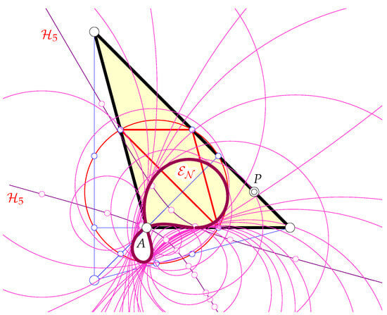
Figure 4. The envelope ${\mathcal{E}}_{\mathcal{N}}$ of the one-parameter family of nine-point circles has an ordinary double point at A. The locus of the nine-point centers $X_5$ is a hyperbola ${\mathcal{H}}_5$ according to Theorem 2.

3.2. Bicentric Pairs

We shall have a look at a special pair of bicentric points instead of browsing through a huge collection. The special pair shall be the pair of Brocard points.

The first Brocard point $B_1$ is common to the three circles $b_A$, $b_B$, and $b_C$, where $b_C$ touches $[B,C]$ at B and passes through A (the other circles are obtained by cyclically replacing the ingredients). In order to determine the second Brocard point, we look for the meet of the circles $c_A$, $c_B$, and $c_C$, where $c_C$ touches $[A,B]$ at A and passes through B, and the other circles are constructed by cyclical shifts of points and tangents. We omit the lengthy representations of $B_1$ and $B_2$ and give the locus of the 1st Brocard points of the triangles in the pencil of triangles by the equation

$$\begin{array}{c}{\mathcal{B}}_1:{sin}^4\alpha {(x^2+y^2)}^2\\ +{sin}^2\alpha (x^2+y^2)\left(sin\alpha (\eta cos\alpha -\xi sin\alpha )x+(({cos}^2\alpha -2)\eta -cos\alpha sin\alpha \xi )y\right)\\ +{\left(\eta sin\alpha (\xi sin\alpha -\eta cos\alpha )x+({\xi }^2{sin}^2\alpha -\xi \eta sin\alpha cos\alpha +{\eta }^2)y\right)}^2=0\end{array}$$

The locus of the 2nd Brocard points of the triangles in the one-parameter family can be described by

$$\begin{array}{c}{\mathcal{B}}_2:{sin}^4\alpha {(x^2+y^2)}^2-{sin}^2\alpha (x^2+y^2)\left(2\xi {sin}^2\alpha x-(2\xi sin\alpha cos\alpha -\eta )y\right)\\ -{sin}^4\alpha ({\xi }^2+{\eta }^2)x^2-sin\alpha (2{sin}^2\alpha cos\alpha {\xi }^2-sin\alpha \xi \eta +cos\alpha (2{cos}^2\alpha -3){\eta }^2)xy\\ +cos\alpha ({sin}^2\alpha cos\alpha {\xi }^2-sin\alpha \xi \eta +cos\alpha (1+{sin}^2\alpha ){\eta }^2)y^2=0\end{array}$$

We can summarize with the following:

Theorem 5.

The 1st and 2nd Brocard points of the triangles in the family $\mathcal{T}$ trace rational and bicircular quartic curves ${\mathcal{B}}_1$ and ${\mathcal{B}}_2$ with ordinary double points at A. ${\mathcal{B}}_1$ one touches the line $[A,B]$, ${\mathcal{B}}_2$ touches the line $[C,A]$ at A.

Figure 5 shows the two bicircular quartics occurring as the loci of the two Brocard points of the triangles in the one-parameter family $\mathcal{T}$ of triangles inscribed in the angle at A.

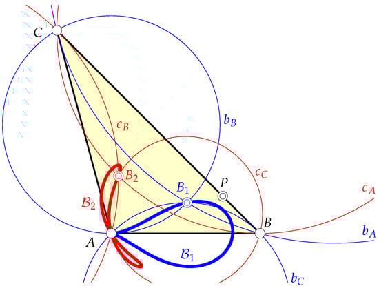
Figure 5. The loci ${\mathcal{B}}_1$ and ${\mathcal{B}}_2$ of the Brocard two points of all triangles in the family are quartic curves sharing the double point at A.

From [10,11], we know that the midpoint of the segment $B_1{B}_2$ is the center $X_{39}$, called the Brocard midpoint. Further, the Brocard circle b is now well-defined as the circumcircle of $\Delta$’s circumcenter $X_3$ and the two Brocard points. The center of b is the triangle center $X_{182}$ usually referred to as the Midpoint of the Brocard Diameter (cf. [10]). Finally, the Symmedian point $X_6$ is the reflection of $X_3$ in $X_{182}$. Figure 6 shows the traces of the triangle centers $X_i$ with $i\in \{3,6,39,182\}$.

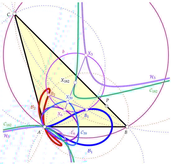
Figure 6. The Brocard points $B_1$ and $B_2$ move on their respective quartics. Meanwhile, the Brocard midpoint $X_{39}$ and the center $X_{182}$ of the Brocard circle trace their own quartics. The Symmedian point $X_6$ has an ellipse ${\mathcal{E}}_6$ for its orbit.

Hence, the orbits of the centers $X_i$ with $i=3,6,39,182$ can now be parametrized and the computation of implicit equations of their orbits is straight forward. Surprisingly, we find:

Theorem 6.

The locus of all Symmedian points $X_6$ of the triangles in the one-parameter family $\mathcal{T}$ is an ellipse ${\mathcal{E}}_6$.

Proof. 

The circumcenter $X_3$ is already determined (cf. (3)) and a parametrization of the orbits of the Brocard points $B_1$ and $B_2$ was computed prior to their implicit equations. Hence, the Brocard midpoint $X_{39}$ which is the midpoint of $B_1$ and $B_2$ is well-defined. (An equation of the quartic curve parametrized by $X_{39}\left(\varphi \right)$ can then be determined by eliminating the parameter $\varphi$. We skip this, because it will not deliver essentially new insight.) The circumcenter of $X_3$ and the two Brocard points $B_1$, $B_2$ equals the center $X_{182}$, which traces a quartic curve passing through the ideal points of the normals to $[A,B]$ and $[C,A]$. Now, the reflection of $X_3$ in $X_{182}$ results in the Symmedian point

$$X_6\left(\varphi \right)=\left({\displaystyle \frac{d(cos(2\alpha -\varphi )+3cos\varphi )}{cos(2\alpha -2\varphi )-cos2\alpha +cos2\varphi +3}},{\displaystyle \frac{d(sin(2\alpha -\varphi )+sin\varphi )}{cos(2\alpha -2\varphi )-cos2\alpha +cos2\varphi +3}}\right),$$

where we have used the abbreviation $d=\xi cos\varphi +\eta sin\varphi$ for the support function of $[B,C]$ once again. The points $X_6\left(\varphi \right)$ lie on the conic with the equation

$$\begin{array}{c}{\mathcal{E}}_6:2(1-cos2\alpha )x^2-6sin2\alpha xy+4(2+cos2\alpha )y^2\\ +\left(\xi \right(cos2\alpha -1)+\eta sin2\alpha )x+(\xi sin2\alpha -\eta (3+cos2\alpha \left)\right)y=0,\end{array}$$

(9)

which is an ellipse independent of the choice of $\alpha \ne 0,\pi$ and for any admissible choice of $P=(\xi ,\eta )$. □

The center of ${\mathcal{E}}_6$ equals the following:

$${\displaystyle \frac{1}{14-2cos\left(2\alpha \right)}}\left((\xi cos(2\alpha )+\eta sin(2\alpha )+5\xi ),(\xi sin(2\alpha )-\eta cos(2\alpha )+3\eta )\right).$$

If $\alpha$ is allowed to run through ${\mathrm{S}}^1$, the latter is a parametrization of an ellipse $e_6$ with the following equation:

$$e_6:8x^2-6\xi x+{\xi }^2+24y^2-10\eta y+{\eta }^2=0$$

centered at $\left({\displaystyle \frac{3}{8}}\xi ,{\displaystyle \frac{5}{24}}\eta \right)$ with principal axes lengths ${\displaystyle \frac{1}{24}}\sqrt{3{\eta }^2+9{\xi }^2}$, ${\displaystyle \frac{1}{24}}\sqrt{{\eta }^2+3{\xi }^2}$. The ellipses ${\mathcal{E}}_6$ pass through $A=(0,0)$ independent of the choice of $\alpha$ and envelop an elliptic quartic ${\mathcal{H}}_6$ if $\alpha$ traces the unit circle. Figure 7 shows some ellipses as orbits of the Symmedian point for triangle pencils with triangle sides $[B,C]$ passing through P and various choices of $\alpha =\angle [C,A],[A,B]$.

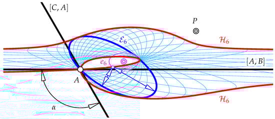
Figure 7. Some ellipses as orbits of $X_6$ in different triangle families $\mathcal{T}$ (variable $\alpha$). One particalur ellipse ${\mathcal{E}}_6$ is emphasized. The orbit $e_6$ of all centers of all $X_6$-orbits is also shown. The quartic ${\mathcal{H}}_6$ is the boundary of the area of all possible Symmedian points $X_6$ of the two-parameter family of triangles (variable $\alpha$ and $[B,C]$ sweeps the pencil about P).

We can collect the latter results:

Theorem 7.

The ellipses ${\mathcal{E}}_6$ as loci of the Symmedian point $X_6$ of all triangles with fixed α at A and side lines $[B,C]$ tracing the pencil about P envelop an elliptic quartic ${\mathcal{H}}_6$ with a double point at A and at the ideal point of $[A,B]$.

Proof. 

We only have to determine an equation of the envelope of all ${\mathcal{E}}_6$ given in (9). This can be performed in the same way as in the case of the envelope of the circumcircles and we find

$$12y^2(x^2+4y^2)-4y(\eta x^2+3\xi \eta xy+10\eta y^2)+{\eta }^2{x}^2+6\xi \eta xy+(8{\eta }^2-{\xi }^2)y^2=0.$$

The ordinary double at A is obvious (no terms of degree lower than 2) and the double point at the ideal point of $[A,B]$ has the two tangents $\eta +6y=0$ and $\eta -2y=0$. □

Figure 7 illustrates the contents of Theorem 7.

4. Traces of Some More Centers

There are some more triangle centers that can be reached with our analytical approach. The course of the incenter is rather unspectacular, since the pair of angle bisectors at A is fixed once $\alpha$ is chosen. The incenter $X_1$ allows for the analytical representation of the form

$$X_1=d\left({\displaystyle \frac{1+cos\alpha }{cos(\alpha -\varphi )+cos\varphi +sin\alpha }},{\displaystyle \frac{sin\alpha }{cos(\alpha -\varphi )+cos\varphi +sin\alpha }}\right).$$

(10)

Similarly, we can give the coordinates of the excenters. Note that the incenter and the excenter that lies on the exterior angle bisector through A interchange their roles as $[B,C]$ is rotating around P and forms the triangle “left” to A. This phenomenon frequently occurs when triangles smoothly change their shapes and orientations (or turn from acute to obtuse), see for example [1,13].

The representation of the incenter given in (10) leads to the vertices $A_i\in [B,C]$ (cyclic) of the intouch triangle ${\Delta }_i$, written as follows:

$$\begin{array}{c}{A}_i={\displaystyle \frac{d}{cos(\alpha -\varphi )+cos\varphi +sin\alpha }}\left(cos\varphi sin\alpha +cos\alpha +1,dsin\alpha (1+sin\alpha )\right),\\ B_i={\displaystyle \frac{d(1+cos\alpha )}{cos(\alpha -\varphi )+cos\varphi +sin\alpha }}\left(cos\alpha ,sin\alpha \right),C_i={\displaystyle \frac{d(1+cos\alpha )}{cos(\alpha -\varphi )+cos\varphi +sin\alpha }}\left(1,0\right).\end{array}$$

(11)

Further, we shall give the coordinates of the excenter $A_1$ opposite to A

$$A_1=\left({\displaystyle \frac{d(cos(\alpha +\varphi )+cos\varphi -sin\alpha )-\eta sin\alpha }{2cos\varphi (cos\varphi -sin\alpha )}},{\displaystyle \frac{-sin\alpha \left(d\right(1+sin\varphi )+\eta )}{cos\varphi cos(\alpha +\varphi )-sin\varphi -cos\alpha -1}}\right)$$

and skip the other two because of the complexity of their coordinate representation, and moreover, because $X_1$ and $A_1$ together with the vertices (1) of $\Delta$ are sufficient in order to find the remaining excenters (if at all necessary).

4.1. Gergonne and Nagel Point

The perspector of $\Delta$ and its intouch triangle ${\Delta }_i$ is referred to as the Gergonne point $X_7$ (cf. [10,11]). With (11), we can find a parametrization of the curve of Gergonne points corresponding to the triangles in $\mathcal{T}$. Then, we implicitize and find

$$\begin{array}{c}{\mathcal{C}}_7:y\left(2ax+(a^2-1)y\right)\left(4x^2+6axy+(1+3a^2)y^2\right)\\ -4y\left(2ax+(a^2-1)y\right)\left((a\eta +2\xi )x+(a\xi +(1+a^2)\eta )y\right)\\ -4\left(a^2{\eta }^2{x}^2-2a({\xi }^2+a\xi \eta +{\eta }^2)xy+({\xi }^2+(1-a^2){\eta }^2)y^2\right)=0.\end{array}$$

The isotomic conjugate of $X_7$ is the Nagel point $X_8$ (cfs. [10,11]). In other words, the Nagel point is also the perspector of $\Delta$ and its extouch triangle ${\Delta }_e$. This leads to a parametrization, and consequently, to the following implicit equation

$$\begin{array}{c}{\mathcal{C}}_8:y(2ax-y)\left(2ax+(a^2-1)y\right)\left(2a^{3}x-(3a^2+1)y\right)\\ -4a^{2}y\left(2ax+(a^2-1)y\right)\left(a(2a\xi -\eta )x+((1+a^2)\eta -a\xi )y\right)\\ -4a^4\left(a^2{\eta }^2{x}^2-2a({\xi }^2+a\xi \eta +{\eta }^2)xy+({\xi }^2+(1-a^2){\eta }^2)y^2\right)=0.\end{array}$$

Both curves ${\mathcal{C}}_7$ and ${\mathcal{C}}_8$ have an ordinary node at A, since A can be viewed as a “singular” triangle in $\mathcal{T}$. Figure 8 shows the curves ${\mathcal{C}}_7$ and ${\mathcal{C}}_8$.

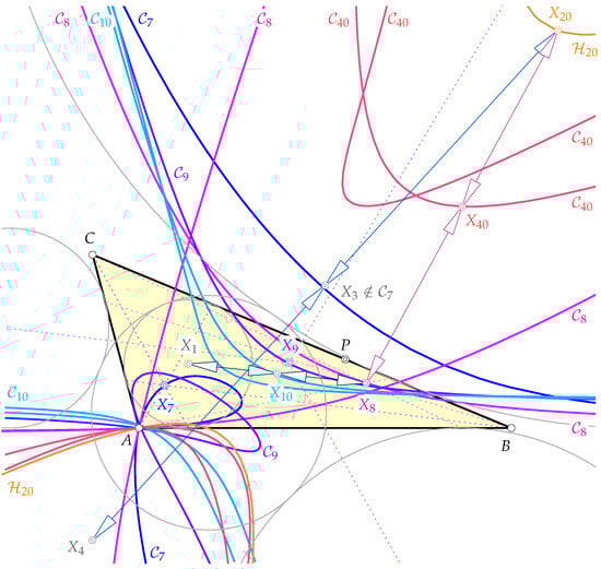
Figure 8. The orbits of $X_7$, $X_8$, and $X_9$ (Gergonne and Nagel point, Mittenpunkt) are quartic curves. The curve ${\mathcal{C}}_{10}$ is a sextic housing all poses of the Spieker point $X_{10}$, while $X_{40}$ moves on a quartic ${\mathcal{C}}_{40}$ and the trace of the de Longchamps point $X_{20}$ is a hyperbola ${\mathcal{H}}_{20}$ according to Theorem 2.

The quadratic factors in the inhomogeneous equations of ${\mathcal{C}}_7$ and ${\mathcal{C}}_8$ agree up to the constant factor $a^4$. Thus, the two quartics also share the tangents at the common double point A.

4.2. Mittenpunkt

The Mittenpunkt $X_9$ is the perspector of the medial triangle ${\Delta }_m$ and the excentral triangle ${\Delta }_e$ (see [10,11]). With (1) and the excenters deduced from (10), we find a parametrization of the trace of the Mittenpunkt, and further, the following equation

$$\begin{array}{c}{\mathcal{C}}_9:y(1+a^2)\left(2ax+(1+a^2)y\right)\left(4x^2+6axy+(1+3a^2)y^2\right)\\ -4a^3\eta x^3-4a\left(2(1+a^2)\xi +3a^3\eta \right)x^{2}y-2\left((1+a^2)(5a^2-2)\xi +a(6a^4+a^2+1)\eta \right)x{y}^2\\ -2\left(a(2a^2-1)(a^2+1)\xi -(2a^6+2a^2+1)\eta \right)y^3\\ a^2\eta \left(2a\xi +(a^2-1)\eta \right)x^2+2a\left((1+a^2){\xi }^2+2a^3\xi \eta +(1+a^4){\eta }^2\right)xy\\ +\left((a^4-1){\xi }^2+2a^5\xi \eta +(a^6-1){\eta }^2\right)y^2=0.\end{array}$$

For a specific assumption on $\alpha$, an example of the quartic curve housing all poses of the Mittenpunkt of the triangles in the family $\mathcal{T}$ is shown in Figure 8.

For the very special choice of $a=-{\displaystyle \frac{\xi }{\eta }}$, i.e., P is chosen on the exterior angle bisector at A, the double point of ${\mathcal{C}}_9$ at A becomes a tacnode with the tangent $\eta y+\xi x=0$ (orthogonal to $[A,P]$ passing through A).

4.3. De Longchamps Point, Bevan Point, Spieker Point

As a point on the Euler line, the de Longchamps point $X_{20}$ travels on a hyperbola (according to Theorem 1) with the following equation:

$$\begin{array}{c}{\mathcal{H}}_{20}:2\left(cos\left(3\alpha \right)+7cos\alpha \right)x^2+\left(3sin\left(3\alpha \right)+7sin\alpha \right)xy\\ -\left(cos\left(3\alpha \right)-cos\alpha \right)y^2+\left(\eta (sin(3\alpha )-3sin\alpha )+2\xi (cos(3\alpha )-2cos\alpha )\right)y\\ +\xi \left(sin\left(3\alpha \right)-3sin\alpha \right)x=0\end{array}$$

which is centered at the following:

$$M_{20}=\left({\displaystyle \frac{1}{sin\alpha }}(\xi sin\alpha -2\eta cos\alpha ),{\displaystyle \frac{1}{cos\left(2\alpha \right)-1}}(2\xi sin\left(2\alpha \right)-3\eta (cos\left(2\alpha \right)-5)\right).$$

The equation of the hyperbola ${\mathcal{H}}_{20}$ can also be found by substituting $w=4$ into (6) and the corresponding implicit equation. The orbit of the centers of all ${\mathcal{H}}_{20}$ for varying angle $\alpha$ is the parabola with vertex $(\xi /2,(4{\eta }^2-{\xi }^2)/\left(4\eta \right))$, axis parallel to the y-axis, and the semi-latus rectum $\eta /2$.

We find the Spieker point $X_{10}$ as the midpoint of the orthocenter $X_4$ and the Bevan point $X_{40}$, cf. [11]. Alternatively, but more intricate from the computational point of view, we could determine $X_{10}$ as the incenter of the medial triangle ${\Delta }_m$. According to [11], the Bevan point is the midpoint of the Nagel point $X_8$ and the de Longchamps point $X_{20}$. Hence, $X_{10}={\displaystyle \frac{1}{2}}(X_4+X_{40})$ and $X_{40}={\displaystyle \frac{1}{2}}(X_8+X_{20})$. Since $X_{20}=X_4\left({\Delta }_a\right)$ (orthocenter of the anti-complementary triangle), $X_{20}$ is the reflection of $X_4$ in $X_3$, and consequently, $X_{20}=2X_3-X_4$. Thus, $X_{10}={\displaystyle \frac{1}{2}}(X_4+{\displaystyle \frac{1}{2}}(X_8+X_{20}))={\displaystyle \frac{1}{2}}(X_4+{\displaystyle \frac{1}{2}}(X_8+2X_3-X_4))={\displaystyle \frac{1}{4}}(2X_3-X_4+X_8)$, which leads to a parametrization of the one-parameter family of Spieker points defined by the triangles in the triangle family $\mathcal{T}$.

The implicitization of the parametrization of the Spieker point $X_{10}\left(\varphi \right)$ shows that it traces the sextic curve ${\mathcal{C}}_{10}$ with the following equation:

$$\begin{array}{c}{\mathcal{C}}_{10}:2^{10}(1+a^2){\left(2ax+(a^2-1)y\right)}^2\left(4x^2+6axy+(1+3a^2)y^2\right)\\ -2^8(1+a^2)y\left(2ax+(a^2-1)y\right)(4a\eta (6a^2+5)x^3\\ +\left(4a(13a^2+15)\xi +2(37a^4+23a^2-10)\eta \right)x^{2}y\\ +\left((64a^4+56a^2-20)\xi +a(75a^4+52a^2-15)\eta \right)x{y}^2\\ +\left(a(25a^4+24a^2-5)\xi +(a^2-1)(25a^4+38a^2+15)\eta \right)y^3)+\dots =0\end{array}$$

up to constant coefficients.

If P is chosen on the exterior angle bisector at A, the ordinary node at A becomes a tacnode. The choice of $P\in [C,A]$ causes ${\mathcal{C}}_{10}$ split into a quartic curve and the repeated line $[C,A]$.

The sextic equation of the orbit ${\mathcal{C}}_{40}$ of the Bevan point $X_{40}$ starts with the following:

$$\begin{array}{c}{\mathcal{C}}_{40}:\left((a^2-1)x-ay\right)\left(2(a^2-1)x-3ay\right)\left((1+a^4)x+a(1-a^2)y\right)\\ \phantom{{\mathcal{C}}_{40}:}·\left(2(a^4+a^2+1)x+a(1-a^2)y\right)\left(4x^2+6axy+(1+3a^2)y^2\right)+\dots =0,\end{array}$$

where constant factors are cut out. The double point at A behaves in a way similar to that on ${\mathcal{C}}_7$, ${\mathcal{C}}_8$, and ${\mathcal{C}}_9$ depending on the choice of P.

4.4. Feuerbach Point and Its $(X_1,X_5)$-Harmonic Conjugate $X_{12}$

The Feuerbach point $X_{11}$ is the point of contact of the nine-point circle and the incircle i of $\Delta$. Since we have already found $X_1$, we also can give an equation of the incircle. Furthermore, the nine-point center $X_5$ is the midpoint of $X_3{X}_4$, the equation of the nine-point circle n (as the circumcircle of the medial triangle) is then also nearby. The computation of the one and only common point of i and n yields a parametrization of the family of all nine-point centers and the subsequent elimination of the parameter $\varphi$ yields an equation of the nine-point orbit, written as follows:

$$\begin{array}{c}{\mathcal{C}}_{11}:(x^2+y^2)\left(8a^{3}x+(3a^4-6a^2-1)y\right)\left((1+3a^2)y-2ax\right)\\ +8a^3(2a\xi +(1-a^2)\eta )x^3-4a((5a^4+2a^2+1)\xi +2a(a^2-1)(a^2-2)\eta )x^{2}y\\ -2((a^2-1)(3a^4+1)\xi +4a(4a^4+a^2-1)\eta )x{y}^2\\ +(4a(1-a^2)(3a^2+1)\xi -2(9a^6-17a^4-a^2+1)\eta )y^3\\ -(4a^4{\xi }^2-4a^3(a^2-1)\xi \eta +a^2{(a^2-1)}^2{\eta }^2)x^2\\ +(2a(2a^4+1){\xi }^2+2a^2(2a^4-2a^2+3)\xi \eta +2a(7a^4-4a^2+1){\eta }^2)xy\\ +((3a^2+1)(a^2-1){\xi }^2+12a^3(a^2-1)\xi \eta +(9a^6-19a^4+7a^2-1){\eta }^2)y^2=0,\end{array}$$

which is a circular quartic curve. The curve ${\mathcal{C}}_{11}$ has three ordinary double points: at A, and further, at the following:

$${\displaystyle \frac{1}{\eta sin\frac{\alpha }{2}+\xi cos\frac{\alpha }{2}}}\left(cos{\displaystyle \frac{\alpha }{2}},sin{\displaystyle \frac{\alpha }{2}}\right)\mathrm{and}\left({\displaystyle \frac{\xi cos\alpha -\eta sin\alpha -2\xi }{2cos\alpha -3}},{\displaystyle \frac{3\eta cos\alpha -\xi sin\alpha -2\eta }{2cos\alpha -3}}\right).$$

The harmonic conjugate of $X_{11}$ with respect to $X_1$ and $X_{12}$ is known as the center $X_{12}$. We shall not write down its implicit equation due to its length. However, the curve ${\mathcal{C}}_{12}$ is a rational quartic with an ordinary double point at A and two further ordinary double points. The curves ${\mathcal{C}}_{11}$ and ${\mathcal{C}}_{12}$ for a particular choice of $\alpha$ can be seen in Figure 9.

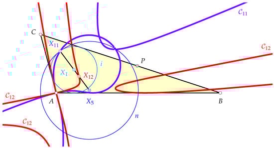
Figure 9. The trace ${\mathcal{C}}_{11}$ of the Feuerbach point $X_{11}$ is a quartic curve. The same holds true for $X_{12}$, the harmonic conjugate of $X_{11}$ with respect to $(X_1,X_5)$.

5. Conclusions and Future Work

The synthetic approach in [6] is by far the most elegant approach. Nevertheless, in some cases it is limited, and the algebraic approach can succeed then. This requires a proper Ansatz, i.e., a suitable way to parametrize the moving and changing objects. We will not claim that there is a unique Ansatz that does the job.

We have seen that triangle centers on the Euler line move on hyperbola while the triangles vary in the family $\mathcal{T}$. Although the Symmedian point $X_6$ is (in general) not located on the Euler line, it moves on an ellipse. It is so far the only point off the Euler line we know to move on a conic, and even on an ellipse. It remains unclear whether there are some more centers behaving that way.

References

- Garcia, R.A.; Odehnal, B.; Reznik, D. Poncelet porisms in hyperbolic pencils of circles. J. Geom. Graph. 2021, 25, 205–225. [Google Scholar]
- Garcia, R.A.; Reznik, D. Loci of the Brocard points over selected triangle families. Int. J. Geom. 2022, 11, 35–45. [Google Scholar]
- Kodrnja, I.; Koncul, H. The Loci of Vertices of Nedian Triangles. KoG 2017, 21, 19–25. [Google Scholar] [CrossRef]
- Kovačević, N.; Sliepčević, A. On the Certain Families of Triangles. KoG 2012, 16, 21–26. [Google Scholar]
- Odehnal, B. Poristic loci of triangle centers. J. Geom. Graph. 2011, 15, 45–67. [Google Scholar]
- Sliepčević, A.; Halas, H. Family of triangles and related curves. Rad HAZU 2013, 515, 203–210. [Google Scholar]
- Jurkin, E. Curves of Brocard Points in Triangle Pencils in Isotropic Plane. KoG 2018, 22, 20–23. [Google Scholar] [CrossRef]
- Jurkin, E. Loci of centers in pencil of triangles in the isotropic plane. Rad Hrvat. Akad. Znan. Umjet. Mat. Znan. 2022, 26, 155–169. [Google Scholar] [CrossRef]
- Žlepalo, M.K.; Jurkin, E. Curves of centroids, Gergonne points and symmedian centers in triangle pencils in isotropic plane. Rad Hrvat. Akad. Znan. Umjet. Mat. Znan. 2018, 22, 119–127. [Google Scholar]
- Kimberling, C. Triangle Centers and Central Triangles; (Congressus Numerantium, Volume 129); Utilitas Mathematica Publishing: Winnipeg, MB, Canada, 1998. [Google Scholar]
- Kimberling, C. Encyclopedia of Triangle Centers. Available online: https://faculty.evansville.edu/ck6/encyclopedia/ETC.html (accessed on 1 June 2025).
- Stachel, H.; Glaeser, G.; Odehnal, B. The Universe of Conics. From the Ancient Greeks to 21st Century Developments; Springer: Berlin/Heidelberg, Germany, 2016. [Google Scholar]
- Wildberger, N.J. Universal affine triangle geometry and four-fold incenter symmetry. KoG 2012, 16, 63–80. [Google Scholar]
Disclaimer/Publisher’s Note: The statements, opinions and data contained in all publications are solely those of the individual author(s) and contributor(s) and not of MDPI and/or the editor(s). MDPI and/or the editor(s) disclaim responsibility for any injury to people or property resulting from any ideas, methods, instructions or products referred to in the content. |
© 2025 by the authors. Licensee MDPI, Basel, Switzerland. This article is an open access article distributed under the terms and conditions of the Creative Commons Attribution (CC BY) license (https://creativecommons.org/licenses/by/4.0/).