Article

A Fokker–Planck Model for Optical Flow Estimation and Image Registration

by
Tudor Barbu
1,2,*,
Costică Moroşanu
3 and
Silviu-Dumitru Pavăl
4
1
Institute of Computer Science of the Romanian Academy—Iasi Branch, Bd. Carol I, No. 8, 700506 Iaşi, Romania
2
Academy of Romanian Scientists, 050044 Bucharest, Romania
3
Faculty of Mathematics, “Al. I. Cuza” University, Bd. Carol I, No. 11, 700506 Iaşi, Romania
4
Faculty of Automatic Control and Computer Engineering, Technical University “Gheorghe Asachi” of Iasi, Str. Prof. dr. doc. Dimitrie Mangeron, nr. 27, 700050 Iaşi, Romania
*
Author to whom correspondence should be addressed.
Mathematics 2025, 13(17), 2807; https://doi.org/10.3390/math13172807
Submission received: 19 June 2025 / Revised: 4 August 2025 / Accepted: 29 August 2025 / Published: 1 September 2025

Abstract

The optical flow problem and image registration problem are treated as optimal control problems associated with Fokker–Planck equations with controller u in the drift term. The payoff is of the form 1 2 | y ( T ) y 1 | 2 + α 0 T | u ( t ) | 4 4 d t , where y 1 is the observed final state and y = y u is the solution to the state control system. Here, we prove the existence of a solution and obtain also the Euler–Lagrange optimality conditions which generate a gradient type algorithm for the above optimal control problem. A conceptual algorithm to compute the approximating optimal control and numerical implementation of this algorithm is discussed.

1. Introduction

The optical flow problem (see [1,2,3,4,5]) consists in finding the velocity field of an object motion on an interval [ 0 , T ] if one knows the final image of the object. Thus, the problem that is treated here leads to an effective motion estimation that can be further applied to the video object detection and tracking tasks. This research is part of a larger computer vision project in that field [6]. In a similar way, the image registration problem in medical analysis is formulated ([7,8,9,10]). Namely, given two images Γ 0 = { m 0 ( x ) ; x 𝒪 } , Γ 1 = { m 1 ( x ) ; x 𝒪 } , where 𝒪 R d , d = 2 , 3 , the registration problem is to find a mapping m : [ 0 , T ] × 𝒪 R such that m ( 0 , x ) = m 0 ( x ) and m ( T , x ) = m 1 ( x ) , x 𝒪 . This mapping generates a continuous flow of images Γ t = { m ( t , x ) ; x 𝒪 } , t [ 0 , T ] , which steers the image Γ 0 in Γ 1 in time T. In the literature on optical flow, as well as of image registration, the mapping m is taken as the brightness of the pattern at point x 𝒪 and at time t. The pattern dynamics is given by the ordinary differential equation
d z d t = u ( t , z ) , t ( 0 , T ) ; z ( 0 ) = z 0 ( x ) , x 𝒪 ,
where u : [ 0 , T ] × 𝒪 𝒪 is a smooth vector-field and z 0 : 𝒪 𝒪 is a given diffeomorphism. Assuming that the brightness m ( t , z ( t ) ) is constant on the trajectory { t ; z ( t ) } , one obtains for m the hyperbolic first-order equation
m t ( t , x ) + u ( t , x ) · x m ( t , x ) = 0 , t [ 0 , T ] , x 𝒪 , m ( 0 , x ) = m 0 ( z 0 1 ( x ) ) = m ˜ 0 ( x ) , x 𝒪 .
Then, the image registration problem reduces to the following exact controllability problem:
Given the functions m ˜ 0 , m ˜ 1 : 𝒪 R , determine the velocity field u : [ 0 , T ] × 𝒪 𝒪 such that
m ( T , x ) = m ˜ 1 ( x ) = m 1 ( z 0 1 ( x ) ) , x 𝒪 .
Optical flow estimation and image registration are treated here as optimal control problems associated with some Fokker–Planck Equations ([11,12]). We shall use a different model by replacing the first-order hyperbolic Equation (2) by the Fokker–Planck equation:
y t ν Δ y + div ( u y ) = 0 in ( 0 , T ) × R d , y ( 0 , x ) = y 0 ( x ) , x R d ,
where ν > 0 and y 0 L 1 ( R d ) L 2 ( R d ) is a probability density [11]. Then, the problem we address here is formulated as follows:
(P)
Given y 1 L 1 ( R d ) L 2 ( R d ) , find the velocity field u : [ 0 , T ] × R d R d such that y ( T , x ) y 1 ( x ) .
In order to write the above problem (3) into this form, one should extend the diffeomorphism z 0 : 𝒪 𝒪 to a diffeomorphism z 0 : R d R d . Such an extension is always possible for smooth domains 𝒪 . An alternative is to replace (4) by a similar problem on 𝒪 with a flux boundary condition (see Remark 1).
It is well known that Equation (4) is equivalent to the stochastic differential equation
d X + u ( t , X ) d t = 2 ν d W , t ( 0 , T ) , . X ( 0 ) = x 0 ,
is a probability space ( Ω , F , F t ) with a d-Brownian motion W [11]. More precisely, if X is a solution to (5) and the probability density L X 0 = y 0 , then y ( t , x ) L X ( t ) , where L X ( t ) is the probability density of the process X ( t ) . Conversely, if X is a solution to (5), then L X ( t ) = y ( x ) is a distributional solution to (4) (see [11], Section 5 for details). Then, in this formulation, the stochastic differential Equation (5) is used, while Equation (2) is replaced by the Fokker–Planck Equation (4). Here, we shall not solve the exact controllability problem (P) but we shall approach it through an optimal control problem ([2,4,7,13,14,15,16]). Such an approach has already been used in optical flow and image registration problems ([10,17]); the main difference is that here the controller u is taken in a larger class of inputs u (see problem (6)).
Notation. 
If 𝒪 is an open set of R d , for 1 p , we denote by L p ( 𝒪 ) = L p the space of all the Lebesgue p-integrable functions on 𝒪 , with the standard norm · L p ( 𝒪 ) denoted | · | p . By H 1 ( 𝒪 ) , we denote the Sobolev space y L 2 ; y x j L 2 , j = 1 , 2 , , d with the standard norm y H 1 ( 𝒪 ) = 𝒪 ( | y | 2 + | y | 2 ) d x 1 2 . Denote by ( H 1 ( 𝒪 ) ) the dual space of H 1 ( 𝒪 ) and by · , · H 1 ( H 1 ) the duality pairing on ( H 1 ( 𝒪 ) ) × H 1 ( 𝒪 ) , which coincide with the scalar product ( · , · ) 2 of L 2 on L 2 ( 𝒪 ) × L 2 ( 𝒪 ) . For T > 0 , we denote by C ( [ 0 , T ] ; L p ( 𝒪 ) ) the space of all L p ( 𝒪 ) -valued continuous functions y : [ 0 , T ] L p ( 𝒪 ) . By L 2 ( 0 , T ; H 1 ( 𝒪 ) ) , we denote the space of functions y : ( 0 , T ) H 1 ( 𝒪 ) with y ( t ) H 1 ( 𝒪 ) L 2 ( 0 , T ) and similarly for the space L 2 ( 0 , T ; L 2 ( 𝒪 ) ) .

2. The Optimal Control Problem

We shall approximate the controllability problem (P) by the optimal control problem [2]:
M i n i m i z e 1 2 | y ( T ) y 1 | 2 2 + α 0 T | u ( t ) | 4 4 d t
subject to u L 4 ( 0 , T ; ( L 4 ( R d ) ) d ) and
y t ν Δ y + div ( u y ) = 0 in 𝒪 T , y ( 0 ) = y 0 in R d .
Here, α is a given positive constant, 𝒪 T = ( 0 , T ) × 𝒪 and Q T = ( 0 , T ) × R d . By definition, a solution y to (7) is a function y : Q T R such that
y C ( [ 0 , T ] ; L 2 ( R d ) ) L 2 ( 0 , T ; H 1 ( R d ) ) ,
d y d t L 2 ( 0 , T ; ( H 1 ( R d ) ) ) ,
d d t R d y ( t , x ) φ ( x ) d x + ν R d y ( t , x ) · φ ( x ) d x R d u ( t , x ) y ( t , x ) · φ ( t , x ) d x = 0 ,   a . e .   t ( 0 , T ) , φ H 1 ( R d ) ,
y ( 0 , x ) = y 0 ( x ) , x R d .
In [18], a similar optimal control problem with quadratic pay-off and free divergence controllers u was used to solve the optical flow problem. The problem (6) is considered here for a larger class of controllers, namely U = L 4 ( 0 , T ; ( L 4 ( R d ) ) d ) , which is an advantage for numerical simulation. This choice of U was dictated by necessity to derive some sharp estimates for the state y of control system (12) necessary to obtain existence in problem (6) and (7).
We have
Lemma 1. 
Let 1 d 3 , y 0 L 2 ( R d ) and u L 4 ( 0 , T ; ( L 4 ( R d ) ) d ) = L 4 ( Q T ) . Then, there is a unique solution y = y u to (7). Moreover,
| y ( t ) | 1 | y 0 | 1 , t ( 0 , T ) ,
and if y 0 𝒫 , then y ( t ) 𝒫 , t ( 0 , T ) , where
𝒫 y 0 L 1 ; y 0 0 , R d y 0 ( x ) d x = 1 .
Proof. 
Assume first that u L ( Q T ) . Then, the existence and uniqueness of a solution is a standard result in the literature. In fact, it follows from existence theory for the Cauchy problem [11]
d y d t + A ( t ) y = 0 , t ( 0 , T ) , y ( 0 ) = y 0 ,
where A ( t ) : H 1 ( H 1 ) is the operator defined by
A ( t ) , φ H 1 ( H 1 ) = ν R d y ( x ) · φ ( x ) d x R d u ( t , x ) y ( x ) · φ ( x ) d x , φ H 1 ,
and, as easily seen,
A ( t ) y H 1 C y H 1 , y H 1 , A ( t ) , y H 1 ( H 1 ) ν 2 y H 1 2 C | y | 2 2 , y H 1 .
Moreover, if y is the solution to (13) (equivalently, (7)), we have
1 2 d d t | y ( t ) | 2 2 + ν | y ( t ) | 2 2 = R d u ( t , x ) y ( t , x ) · y ( t , x ) d x ,   a . e .   t ( 0 , T ) .
Conversely, we have by Schwartz inequality
R d | u y · y | d x | u y | 2 | y | 2 | u | 4 | y | 4 | y | 2 .
Next, by the interpolation inequality | y | 4 C | y | 2 1 2 | y | 6 1 2 combined with Sobolev embedding theorem in R 3 , we have
| y | 4 C | y | 2 1 2 | y | 6 1 2 C | y | 2 1 2 y H 1 1 2 .
This yields via Hölder inequality
R d | u y · y | d x C | u | 4 | y | H 1 3 2 | y | 2 1 2 ν 2 | y | 2 2 + C 1 | u | 4 4 | y | 2 2 .
Substituting in (14), we get
| y ( t ) | 2 2 + ν 0 t | y ( s ) | 2 2 d s C 2 0 t | u ( s ) | 4 4 | y ( s ) | 2 2 d s + | y 0 | 2 2 .
and so, by Gronwall’s lemma,
| y ( t ) | 2 2 + 0 t | y ( s ) | 2 2 d s | y 0 | 2 2 exp C 2 0 T | u ( t ) | 4 4 d t , t [ 0 , T ] .
Now, if u L 4 ( 0 , T ; L 4 ) , we approximate it by u ε = u 1 + ε | u | L ( Q T ) . Then, for the corresponding solution y ε = y u ε to (6), we have estimate (15) and so { y ε } is bounded in L 2 ( 0 , T ; H 1 ) , d y ε d t is bounded in L 2 ( 0 , T ; ( H 1 ) ) and so, by the Aubin–Lions compactness theorem [18], { y ε } is compact in L 2 ( 0 , T ; L 2 ) and weakly compact in L 2 ( 0 , T ; H 1 ) [19]. Hence, on a subsequence, we have
y ε y strongly in L 2 ( 0 , T ; L 2 ) weakly in L 2 ( 0 , T ; H 1 ) d y ε d t d y d t weakly in L 2 ( 0 , T ; ( H 1 ) ) Δ y ε Δ y weakly in L 2 ( 0 , T ; ( H 1 ) ) .
Moreover, we also have
u ε u weakly in L 4 ( 0 , T ; L 4 )
and since { y ε u ε } is bounded in L 2 ( 0 , T ; L 2 ) , we also have
y ε u ε y u weakly in L 2 ( 0 , T ; L 4 ) .
Then, letting ε 0 in Equation (6), where u = u ε , we see that y = y u is a solution to (6) as desired. Now, if we multiply (6), where u = u ε , by sgn u ε and integrate we get
| y ε ( t ) | 1 | y 0 | 1 , t [ 0 , T ] , ε > 0 ,
and, if y 0 𝒫 , then, as easily seen, y ε 0 and
R d y ε ( t , x ) d x = R d y 0 d x = 1 .
Then, for ε 0 , we get (12) and that y ( t ) 𝒫 if y 0 𝒫 .    □
As regards the optimal control problem (6) and (7), we have
Theorem 1. 
Let y 0 L 2 and 1 d 3 . Then, there is at least one solution u * L 4 ( 0 , T ; L 4 ) to the optimal control (6). Moreover, if y 0 𝒫 , then y * ( t ) = y u * ( t ) 𝒫 , t [ 0 , T ] .
Proof. 
Let
I = inf u 1 2 | y u ( T ) y 1 | 2 2 + α 0 T | u ( t ) | 4 4 d t
and let { u n } L 4 ( 0 , T ; L 4 ) be such that
I | y u n ( T ) y 1 | 2 2 + α 0 T | u n ( t ) | 4 4 d t I + 1 n .
By estimate (15), it follows that { y n = y u n } is bounded in L 2 ( 0 , T ; H 1 ) and d y n d t is bounded in L 2 ( 0 , T ; ( H 1 ) ) . Hence, by the Aubin–Lions compactness theorem [18], on a subsequence { n } , we have
y n y * strongly in L 2 ( 0 , T ; L 2 ) and weakly in L 2 ( 0 , T ; H 1 ) , d y n d t d y * d t weakly in L 2 ( 0 , T ; ( H 1 ) ) , Δ y n Δ y * weakly in L 2 ( 0 , T ; ( H 1 ) ) , u n u * weakly in L 4 ( 0 , T ; L 4 ) .
Hence, y n u n y * u * weakly in L 2 ( Q T ) and by (10), where y = y 0 , u = u n , we see that y * = y u * is the solution to (6) with u = u * . Then, letting n in (17), we get
I = | y * ( T ) y 1 | 2 2 + α 0 T | u * ( t ) | 4 4 d t ,
as desired.   □
Remark 1. 
If in problem (6) one replaces R d by a domain 𝒪 R d , the control system (7) should be replaced by
y t ν Δ y + div ( u y ) = 0 in   𝒪 T , ν y ν + ( u · n ) y = 0 in   ( 0 , T ) × 𝒪 y ( 0 ) = y 0
where n is the outward normal to 𝒪 . Theorem 1 remains true by the same argument in this situation.

3. The Euler–Lagrange Optimality System

Consider the backward-dual equation associated with (7),
p * t + ν Δ p * u * · p * = 0 in   Q T , p * ( T ) = ( y * ( T ) y 1 ) in   R d ,
where u * is optimal in problem (6). We have
Theorem 2. 
Let ( y * , u * ) be optimal in problem (6). Then,
u * ( t , x ) = p * ( x ) y * ( t , x ) ( 4 α ( | p * ( t , x ) | | y * ( t , x ) | ) ) 2 3 , a . e . ( t , x ) Q T ,
where p is the solution to (19).
Proof. 
We set
z λ = 1 λ ( y u * + λ v y u * ) , v L 4 ( Q T )
and note that
z λ t ν Δ z λ + div ( v y u * + λ v ) + div ( u * z λ ) = 0   in   Q T , z λ ( 0 ) = 0   in   R d .
If we multiply by z λ and integrate on ( 0 , t ) × R d , we get the estimate (see (15))
| z λ ( t ) | 2 2 + 0 t | z λ ( s ) | 2 2 d s + d z λ d t L 2 ( 0 , T ; ( H 1 ) ) 2 C , t ( 0 , T ) .
Hence, for λ 0 , we have
z λ z v strongly in L 2 ( Q T ) , weakly in L 2 ( 0 , T ; H 1 ) , d z λ d t d z v d t weakly in L 2 ( 0 , T ; p ( H 1 ) ) ,
where z v is the solution to the equation
d z v d t ν Δ z v + div ( u * z v ) + div ( v y * ) = 0   in   Q T , z v ( 0 ) = 0   in   R d .
Conversely, we have
1 2 | y u * ( T ) y 1 | 2 2 + α 0 T | u * ( t ) | 4 4 d t 1 2 | y u * + λ v ( T ) y 1 | 2 2 + α 0 T | u * ( t ) + λ v ( t ) | 4 4 , λ R , v L 4 ( Q T ) ,
and, therefore,
( z v ( T ) , y * ( T ) y 1 ) 2 + 4 α Q T ( u * · v ) | u * | 2 d t d x = 0 , v L 4 ( Q T ) ,
while, by (19) and (22), we have
( z v ( T ) , y * ( T ) y 1 ) 2 Q T y * ( v · p * ) d t d x = 0 , v L 4 ( Q T ) .
This yields
Q T ( 4 α u * | u * | 2 y * p * ) · v d t d x = 0 , v L 4 ( Q T ) ,
and so (20) follows.   □
Equations (7), (19), and (20) taken together lead to the Euler–Lagrange system
y * t ν Δ y * + div ( u * y ) = 0 in   Q T , p * t ν Δ p * u * · p * = 0 in   Q T , y * ( 0 ) = y 0 , p * ( T ) = ( y * ( T ) y 1 ) in   Q T ,
which represents the first and necessary conditions of optimality for problem (6). In particular, by (23), we get that
( p * ( T ) , y * ( T ) ) 2 = 1 ( 4 α ) 2 3 Q T | p * | 4 3 | y * | 4 3 d t d x
and, therefore, we have the inequality
| y * ( T ) y 1 | 2 2 + 1 ( 4 α ) 2 3 Q T | p * | 4 3 | y * | 4 3 d t d x = ( y * ( T ) y 1 , y 1 ) 2 .

4. The Gradient Algorithm

If we denote by Φ : L 4 ( Q T ) R , the payoff function
Φ ( u ) = 1 2 | y u ( T ) y 1 | 2 2 + α Q T u 4 d t d x
its Gâteaux differential
Φ : ( L 4 ( Q T ) ) d ( L 4 3 ( Q T ) ) d
is given by (see (22))
Φ ( u ) , v L 4 ( Q T ) L 4 3 ( Q T ) = lim λ 0 1 λ ( Φ ( u + λ v ) Φ ( u ) ) = ( z v ( T ) , y ( T ) y 1 ) 2 + 4 α Q T ( u · v ) | u | 2 d t d x = Q T ( 4 α u | u | 2 y p ) · v d t d x , v L 4 ( Q T )
and, therefore,
Φ ( u ) = 4 α u | u | 2 y u p , u L 4 ( Q T ) ,
where p is the solution to the equation
p t + ν Δ p u · p = 0 in   Q T , p ( T ) = ( y u ( T ) y 1 ) .
In terms of Φ , the optimality system (3.5) can be rewritten as
Φ ( u * ) = 0 .
Taking into account (24) for a fixed γ > 0 , the explicit gradient algorithm for computing the optimal controller u * is
u n + 1 = u n γ Φ ( u n ) ,
that is,
u n + 1 = u n 4 γ α u n | u n | 2 + y n p n in   Q T , y n t ν Δ y n + div ( u n y n ) = 0 ,
p n t + ν Δ p n u n · p n = 0 in   Q T , y n ( 0 ) = y 0 , p n ( T ) = ( y n ( T ) y 1 ) .

5. Numerical Approximation

In this section, we present some conceptual algorithms of the gradient type in order to compute the approximating optimal control u * of the following problem
M i n i m i z e Φ ( u ) = 1 2 𝒪 y ( T , x ) y 1 ( x ) 2 d x + α 0 T 𝒪 u ( t , x ) 4 d t d x
subject to
t y ν Δ y + div ( u y ) = 0 in   Q T , ν y ν + ( u · n ) y = 0 in   ( 0 , T ) × 𝒪 y ( 0 , x ) = y 0 ( x ) on   𝒪 .
On the basis of Theorem 2, we know that the optimal control u * in problem (29) is given by
u * ( t , x ) = p * ( t , x ) y * ( t , x ) 4 α | p * ( t , x ) | | y * ( t , x ) | 2 3 , a . e . ( t , x ) Q T ,
where p satisfies the adjoint state equation
t p + ν Δ p u · p = 0 in   Q T , p ( T , x ) = y ( T , x ) y 1 ( x ) on   I R d .
We have developed two numerical algorithms to approximate the problem (29)–(32): the finite difference method ([1,16,20]) and 2D explicit difference method. We consider d = 2 and assume that 𝒪 I R 2 is a polygonal domain.

5.1. The Finite Difference Method

Given a positive value T and considering M as the number of equidistant nodes in which is divided the time interval [ 0 , T ] , we set
t i = ( i 1 ) ε , i = 1 , 2 , , M , ε = T / ( M 1 ) .
The problems (30) and (32) will be discretized on the 2D rectangular domain 𝒪 = [ 0 , a ] × [ 0 , b ] I R 2 . Let us denote x = ( x 1 , x 2 ) a generic point in 𝒪 ; we will build a grid on 𝒪 by considering equidistant discretization nodes for both axis O x 1 and O x 2 (see Figure 1). Thus, we discretize [ 0 , a ] by
J x 1 = x 1 0 , x 1 1 , , x 1 j , , x 1 J , x 1 j = j h 1 , j = 0 , 1 , , J , with h 1 = a J ,
and [ 0 , b ] by
K x 2 = x 2 0 , x 2 1 , , x 2 k , , x 2 K , x 2 k = k h 2 , k = 0 , 1 , , K , with h 2 = b K .
The set (cartesian product)
J x 1 × K x 2 = { ( x 1 j , x 2 k ) , x 1 j J x 1 , x 2 k K x 2 , j = 0 , , J , k = 0 , , K }
provides the computational grid on 𝒪 .
Let us denote by y j , k i the approximate values in the points ( t i , x 1 j , x 2 k ) of the unknown function y ( t , x ) in (30), i.e.,
y j , k i = y ( t i , x 1 j , x 2 k ) , ( t i , x 1 j , x 2 k ) Q = { t 1 , t 2 , , t M } × J x 1 × K x 2 ,
or, for later use
y i = y 1 , 1 i , y 2 , 1 i , , y J x 1 , K x 2 i T , i = 1 , 2 , , M .
Corresponding to the initial condition (30)2, we have
y j , k 1 = y ( 0 , x 1 j , x 2 k ) = y 0 ( x 1 j , x 2 k ) , j = 0 , 1 , , J , k = 0 , 1 , , K .
To approximate the partial derivatives with respect to time, t y ( t , x 1 , x 2 ) and t p ( t , x 1 , x 2 ) , we employed a first-order scheme, that is:
t y ( t i + 1 , x 1 j , x 2 k ) y j , k i + 1 y j , k i ε , t p ( t i + 1 , x 1 j , x 2 k ) p j , k i + 1 p j , k i ε ,
i = 1 , 2 , , M 1 , j = 0 , 1 , , J , k = 0 , 1 , , K .

5.2. 2D Explicit Difference Method

The partial differential equation in (30)1 can be written equivalently in the form   
t y ( t , x ) = ν Δ y ( t , x ) x 1 u ( t , x ) y ( t , x ) + x 2 u ( t , x ) y ( t , x ) = ν Δ y ( t , x ) x 1 u ( t , x ) + x 2 u ( t , x ) y ( t , x ) + u ( t , x ) x 1 y ( t , x ) + x 2 y ( t , x ) .
Using (35)1, we get an explicit difference scheme for approximation of (36), as follows
y j , k i + 1 y j , k i ε = ν Δ y j , k i x 1 u j , k i + x 2 u j , k i y j , k i u j , k i x 1 y j , k i + x 2 y j , k i ,
i = 1 , 2 , , M 1 , j = 0 , 1 , , J , k = 0 , 1 , , K .
The laplacian Δ y j , k i is approximated by a central finite difference formula
Δ y j , k i = y j 1 , k i 2 y j , k i + y j + 1 , k i h 1 2 + y j , k 1 i 2 y j , k i + y j , k + 1 i h 2 2
while, to approximate the partial derivatives of u j , k i and y j , k i with respect to x 1 and x 2 , we shall use backward difference formula:
x 1 u j , k i = u j + 1 , k i u j , k i h 1 , j = 0 , 1 , , J 1 , k = 0 , 1 , , K , x 2 u j , k i = u j , k + 1 i u j , k i h 2 , j = 0 , 1 , , J , k = 0 , 1 , , K 1 , x 1 y j , k i = y j + 1 , k i y j , k i h 1 , j = 0 , 1 , , J 1 , k = 0 , 1 , , K , x 2 y j , k i = y j , k + 1 i y j , k i h 2 , j = 0 , 1 , , J , k = 0 , 1 , , K 1 .
Finally, one obtains the following explicit numerical approximation scheme for (30)
y j , k i + 1 = 1 ε u j + 1 , k i u j , k i h 1 + u j , k + 1 i u j , k i h 2 y j , k i + ε ν y j 1 , k i 2 y j , k i + y j + 1 , k i h 1 2 + y j , k 1 i 2 y j , k i + y j , k + 1 i h 2 2 ε u j , k i y j + 1 , k i y j , k i h 1 + y j , k + 1 i y j , k i h 2 ,
i = 1 , 2 , , M 1 , j = 0 , 1 , , J , k = 0 , 1 , , K .
We continue by treating the adjoint state p ( t , x ) in (32). Let us denote by p j , k i the approximate values in the points ( t i , x 1 j , x 2 k ) of the unknown function p ( t , x ) , i.e.,
p j , k i = p ( t i , x 1 j , x 2 k ) , ( t i , x 1 j , x 2 k ) Q = { t 1 , t 2 , , t M } × J x 1 × K x 2 ,
or, for later use
p i = p 1 , 1 i , p 2 , 1 i , , p J x 1 , K x 2 i T , i = 1 , 2 , , M .
Corresponding to the final condition (32)2, we have    
p j , k M = y 1 j , k y j , k M , j = 0 , 1 , , J , k = 0 , 1 , , K ,
where y 1 j , k = y 1 ( x 1 j , x 2 k ) , j = 0 , 1 , , J , k = 0 , 1 , , K (see (29)).
The partial differential equation in (32)1 can be written equivalently in the form    
t p ( t , x ) = ν Δ p ( t , x ) + u ( t , x ) x 1 y ( t , x ) + x 2 y ( t , x ) .
Using (35)2, we get an explicit difference scheme for approximation of (40), as follows
p j , k i + 1 p j , k i ε = ν Δ p j , k i + 1 + u j , k i + 1 x 1 y j , k i + 1 + x 2 y j , k i + 1 ,
i = M 1 , , 2 , 1 , j = 0 , 1 , , J , k = 0 , 1 , , K .
   The laplacian Δ p j , k i is approximated by a central finite difference formula, that is
Δ p j , k i = p j 1 , k i 2 p j , k i + p j + 1 , k i h 1 2 + p j , k 1 i 2 p j , k i + p j , k + 1 i h 2 2 , i = M , , 3 , 2 ,
while, to approximate the partial derivative of y j , k i with respect to x 1 and x 2 , we shall use backward difference formula:
x 1 y j , k i = y j + 1 , k i y j , k i h 1 , j = 0 , 1 , , J 1 , k = 0 , 1 , , K , x 2 y j , k i = y j , k + 1 i y j , k i h 2 , j = 0 , 1 , , J , k = 0 , 1 , , K 1 ,
i = M , , 3 , 2 .
Thus, we get a first explicit numerical approximation scheme for (32)
p j , k i = p j , k i + 1 + ε ν p j 1 , k i + 1 2 p j , k i + 1 + p j + 1 , k i + 1 h 1 2 + p j , k 1 i + 1 2 p j , k i + 1 + p j , k + 1 i + 1 h 2 2 ε u j , k i + 1 y j + 1 , k i + 1 y j , k i + 1 h 1 + y j , k + 1 i + 1 y j , k i + 1 h 2 .
Now we are in position to present a conceptual algorithm (Algorithm 1) of gradient type (see [13,14,15,16] for more details) to compute the approximating optimal control u * ( t , x ) , ( t , x ) Q T , stated by Theorem 2.
Algorithm 1: Algorithm OCP_FP_EDM (Optimal Control Problem—FokkerPlanck_EDM 2D)
P0.
       Set i t e r = 0 ;
       Choose T > 0 , M > 0 and compute ε (see (33));
       Choose a > 0 , J > 0 and compute h 1 ;
       Choose b > 0 , K > 0 and compute h 2 ;
       Choose u j , k i t e r , j = 0 , 1 , , J , k = 0 , 1 , , K ;
       Choose y 1 ( x ) , x 𝒪 I R 2 (see (29));
       Choose y 0 ( x 1 , x 2 ) , ( x 1 , x 2 ) 𝒪 and compute
                    y j , k 1 , j = 0 , 1 , , J , k = 0 , 1 , , K (see (34));
P1.  Determine y j , k i + 1 , i = 1 , 2 , , M 1 , j = 0 , 1 , , J , k = 0 , 1 , , K (see (38));
P2.  Determine p j , k i , i = M 1 , , 2 , 1 , j = 0 , 1 , , J , k = 0 , 1 , , K (see (42));
P3.  Compute u ˜ j , k i t e r = u j , k i t e r 4 γ α u j , k i t e r | u j , k i t e r | 2 + y j , k i + 1 p j , k i (see (4.4));
P4.  Compute λ i t e r [ 0 , 1 ] solution of the minimization process:
min { Φ ( λ u i t e r + ( 1 λ ) u ˜ i t e r , λ [ 0 , 1 ] ;
     Set u i t e r + 1 = λ i t e r u i t e r + ( 1 λ i t e r ) u ˜ i t e r ;
P5.  If u i t e r + 1 u i t e r η                                                 /* the stopping criterion */
          then STOP
     else
          iter : = iter + 1 ; Go to P1.
In the above, the variable iter represents the number of iterations after which the algorithm OCP_FP_EDM found the optimal value of the cost functional Φ ( u ) in (29).
Remark 2. 
The stopping criterion in P5 could be
Φ ( u i t e r + 1 ) Φ ( u i t e r )   η ,
where η is a prescribed precision.

6. Numerical Experiments

In this section, we validate the explicit finite–difference implementation of the optimal-control algorithm OCP_FP_EDM described in the previous section. We detail the discretization, and comment on the numerical results obtained for a simple benchmark based on two smooth Gaussian densities.
The dual purpose of this section is to (a) verify the correctness of our forward/adjoint implementation on a benchmark that admits a smooth solution, and (b) document the practical limitations that arise when the control is driven by an explicit time-stepping scheme.

6.1. Discrete Setting and Algorithmic Details

The computational domain is the unit square 𝒪 = [ 0 , 1 ] × [ 0 , 1 ] R 2 , discretized on a uniform grid with J = K = 64 nodes per spatial direction. The spacings are, therefore,
h x = h y = h = 1 63 1.58 × 10 2 .
The final time is T = 1 and we start with M = 100 time steps Δ t = T / M = 10 2 . At every outer optimal–control iteration we recompute a CFL-adapted time step
Δ t adap = min Δ t , 0.4 | u x | h x + | u y | h y + 2 ν ( h x 2 + h y 2 ) 1 ,
where | u x | : = max i , j | u x , i j | and similarly for u y . The number of sub-steps is M adap = T / Δ t adap , which is the classical CFL bound for a linear advection–diffusion equation. This value replaces the initial choice Δ t = T / 100 whenever it is smaller.
For the Fokker–Planck state Equation (30) and the adjoint Equation (32) we use standard second-order central differences for Δ and first-order (upwind) backward differences for the flux terms. Dirichlet homogeneous boundary conditions ( y = p = 0 ) are enforced on 𝒪 .
Given the current iterate ( y , p , u ) , we compute the point-wise gradient
g = 4 α u | u | 2 y p
and update with a fixed gradient step u new = u γ g .
The value α = 10 3 was selected so that α 0 T 𝒪 | u | 4 d x d t and 1 2 y ( T ) y 1 L 2 2 are of the same order of magnitude in the initial iterate; this prevents the search direction from being dominated by either term.
All parameters used in the run reported below are summarized in Table 1.

6.2. Benchmark Configuration

The initial and target densities are smooth, normalized Gaussians
y 0 ( x ) = exp | x μ 0 | 2 2 σ 2 , y 1 ( x ) = exp | x μ 1 | 2 2 σ 2 ,
with centres μ 0 = ( 0.4 , 0.5 ) , μ 1 = ( 0.6 , 0.5 ) and standard deviation σ = 0.1 . After discretization both images are normalized so that i , j y 0 , i j h x h y = 1 = i , j y 1 , i j h x h y .
The optimization is initialized with a small random perturbation of the control field: u 0 = 0.1 · N ( 0 , 1 ) , where N ( 0 , 1 ) represents independent Gaussian random variables with zero mean and unit variance. This random initialization breaks the symmetry of the zero initial guess and accelerates convergence by providing non-trivial gradient information from the first iteration.

6.3. Results

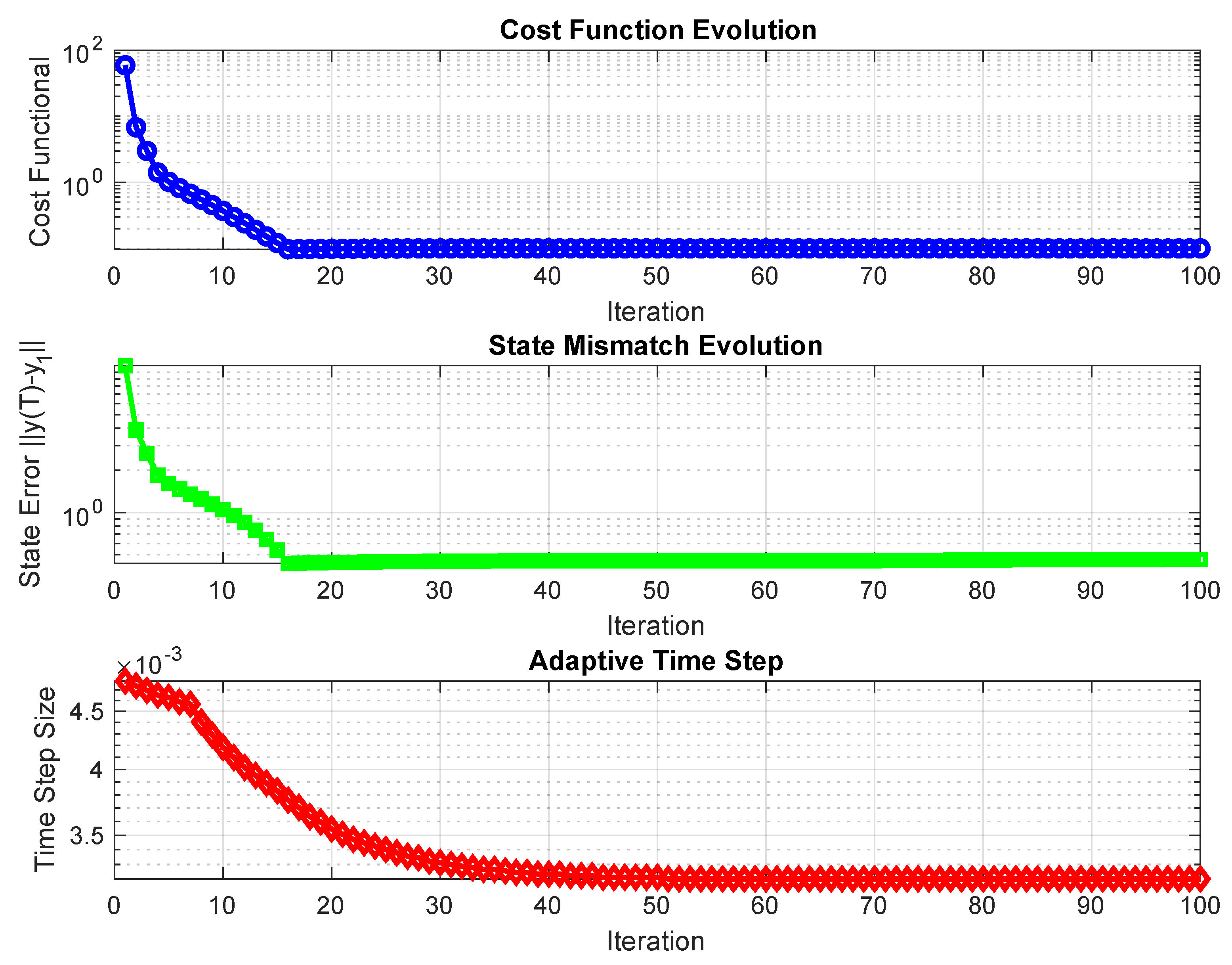
The explicit implementation demonstrates good convergence behavior and achieves successful optimal transport between the specified Gaussian distributions. Table 2 summarizes the quantitative performance metrics over 100 optimization iterations.
The algorithm exhibits robust monotonic convergence in both cost functional and state tracking error. As shown in Figure 2, the cost functional Φ ( u ) decreases exponentially from an initial value of 59.22 to a final value of 0.10.
The state mismatch y ( T ) y 1 L 2 demonstrates consistent improvement throughout the optimization process, reducing from 11.16 to 0.46. This error reduction confirms that the algorithm successfully drives the final state y ( T ) toward the target distribution y 1 . The smooth convergence curves indicate stable numerical behavior without oscillations or stagnation.
The adaptive time stepping mechanism maintains computational efficiency while ensuring CFL stability.
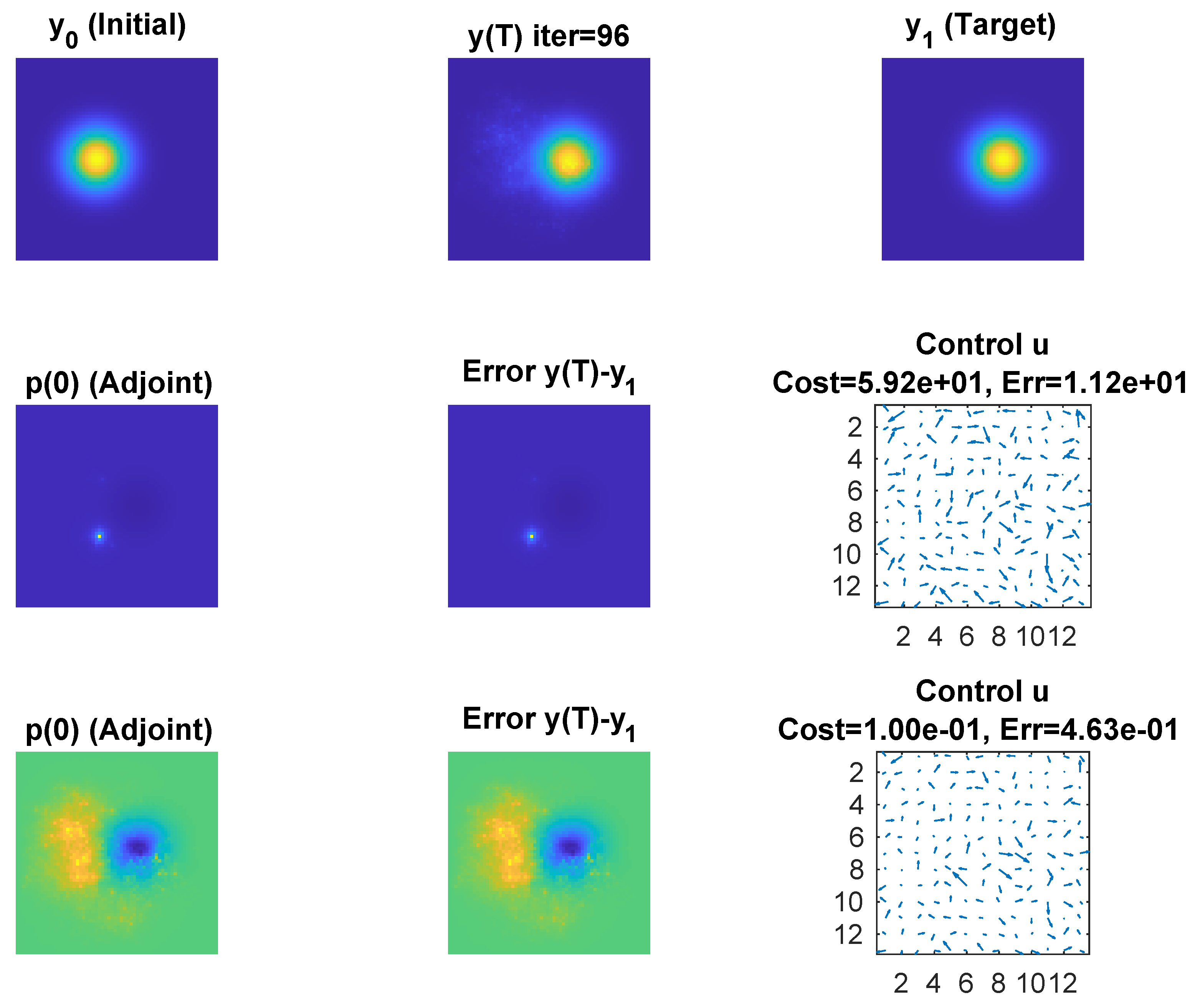
Figure 3 illustrates the complete optimal control solution after convergence. The top row demonstrates successful transport of the Gaussian probability mass from the initial position ( 0.4 , 0.5 ) to the target location ( 0.6 , 0.5 ) . The final state y ( T ) closely approximates the target distribution y 1 , with the residual mismatch y ( T ) y 1 showing only small deviations concentrated near the distribution boundaries.
The adjoint field p ( 0 ) exhibits the expected dual structure, with positive values driving mass away from the source region and negative values attracting mass toward the target. This dual behavior reflects the optimality conditions and provides the gradient information necessary for effective control updates.

7. Discussion

The present experiment confirms that the finite difference discretization and the adjoint implementation are consistent, and it highlights the practical difficulties of gradient-type control when used with explicit solvers.
As already mentioned, the research described in this work is part of the project in the traffic monitoring domain, which is acknowledged below. Thus, the proposed video optical flow estimation can be applied successfully to the detection and tracking of various moving objects, such as pedestrians and vehicles (see [1,6]). Therefore, some video detection and tracking frameworks based on this technique will also represent the focus of our future research in this project.

Author Contributions

Methodology, T.B. and S.-D.P.; Software, C.M. and S.-D.P.; Validation, C.M.; Investigation, S.-D.P. All authors have read and agreed to the published version of the manuscript.

Funding

This research work was supported by a grant of the Romanian Academy, GAR-2023, Project Code 19.

Data Availability Statement

The original contributions presented in this study are included in the article. Further inquiries can be directed to the corresponding author.

Conflicts of Interest

The authors declare no conflicts of interest.

References

  1. Barbu, T. Digital Image Processing, Analysis and Computer Vision Using Nonlinear Partial Differential Equations; Springer Nature: Berlin/Heidelberg, Germany, 2025; Volume 1211. [Google Scholar]
  2. Barbu, V.; Marinoschi, G. An optimal control approach to the optimal flow problem. Syst. Control Lett. 2016, 87, 1–6. [Google Scholar] [CrossRef]
  3. Barron, J.L.; Fleet, D.J.; Beauchemin, S.S. Performance of optical flow techniques. Int. J. Comput. Vis. 1994, 12, 43–77. [Google Scholar] [CrossRef]
  4. Borzi, A.; Itô, K.; Kunish, K. Optimal control formulation for determining optical flow. SIAM J. Comput. 2002, 34, 818–847. [Google Scholar] [CrossRef]
  5. Horn, B.P.K.; Schunk, B.G. Determining optical flow. Artif. Intell. 1981, 17, 185–203. [Google Scholar] [CrossRef]
  6. Barbu, T. Deep learning-based multiple moving vehicle detection and tracking using a nonlinear fourth-order reaction-diffusion based multi-scale video object analysis. Discret. Contin. Dyn.-Syst.-Ser. S AIMS J. 2023, 16, 16–32. [Google Scholar] [CrossRef]
  7. Lee, E.; Gunzburger, M. An optimal control formulation of an image registration problem. J. Math. Vision 2010, 36, 69–80. [Google Scholar] [CrossRef]
  8. Mang, A.; Gholami, A.; Davatzikos, C.; Biros, G. CLAIRE: A Distributed-Memory Solver for Constrained Large Deformation Diffeomorphic Image Registration. SIAM J. Sci. Comput. 2019, 41, C548–C584. [Google Scholar] [CrossRef] [PubMed]
  9. Mang, A.; Gholami, A.; Davatzikos, C.; Biros, G. PDE-constrained optimization in medical image analysis. Optim. Eng. 2018, 19, 765–812. [Google Scholar] [CrossRef]
  10. Zhang, J.; Li, Y. Diffeomorphic image registration with an optimal control relaxation and its implementation. SIAM J. Imaging Sci. 2021, 14, 1890–1931. [Google Scholar] [CrossRef]
  11. Barbu, V.; Röckner, M. Nonlinear Fokker–Planck Flows and their Probabilistic Counterparts; Lecture Notes in Mathematics; Springer: Berlin/Heidelberg, Germany, 2024; Volume 2353. [Google Scholar]
  12. Jordan, R.; Kinderlehrer, D.; Otto, F. The variational formulation of the Fokker–Planck equation. SIAM J. Math. Anal. 1998, 29, 1–17. [Google Scholar] [CrossRef]
  13. Benincasa, T.; Favini, A.; Moroşanu, C. A Product Formula Approach to a Non-homogeneous Boundary Optimal Control Problem Governed by Nonlinear Phase-field Transition System. PART II: Lie-Trotter Product Formula. J. Optim. Theory Appl. 2011, 148, 31–45. [Google Scholar] [CrossRef]
  14. Hömberg, D.; Krumbiegel, K.; Rehberg, J. Optimal control of a parabolic equation with dynamic boundary conditions. Appl. Math. Optim. 2013, 67, 3–31. [Google Scholar] [CrossRef]
  15. Moroşanu, C. Boundary optimal control problem for the phase-field transition system using fractional steps method. Control Cybern. 2003, 32, 5–32. [Google Scholar]
  16. Moroşanu, C. Analysis and Optimal Control of Phase-Field Transition System: Fractional Steps Methods; Bentham Science Publishers: Potomac, MD, USA, 2012. [Google Scholar] [CrossRef]
  17. Lee, J.; Bertr, N.P.; Rozell, C.J. Unbalanced Optimal Transport Regularization for Imaging Problems. IEEE Trans. Comput. Imaging 2020, 6, 1219–1232. [Google Scholar] [CrossRef]
  18. Lions, J.L. Quelques Méthods de Résolution des Problèmes aux Limites Nonlinéaires; Dunod. Gauthier-Villars: Paris, France, 1969. [Google Scholar]
  19. Simon, J. Compact sets in the space Lp(O,T;B). Ann. Mat. Pura Appl. 1986, 146, 65–96. [Google Scholar] [CrossRef]
  20. Boole, G. Calculus of Finite Differences; BoD–Books on Demand; Salzwasser-Verlag: Bremen, Germany, 2022. [Google Scholar]
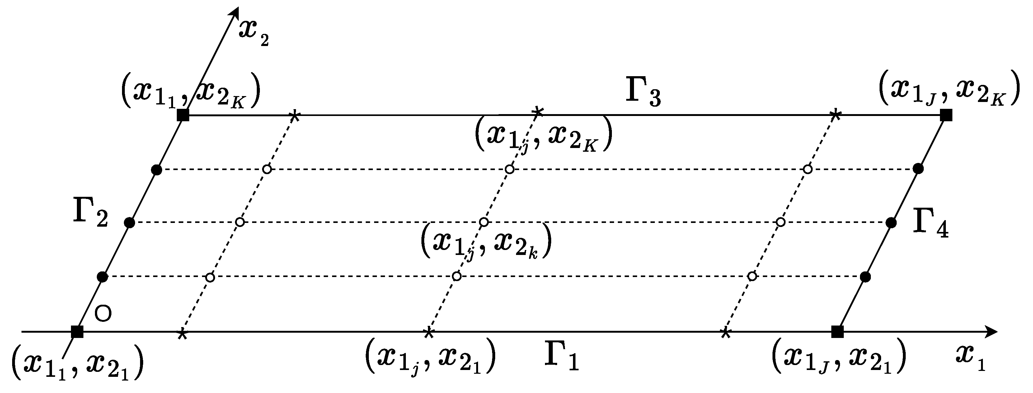
Figure 1. The boundary Γ = = 1 4 Γ of the rectangle 𝒪 = [ 0 , a ] × [ 0 , b ] .
Mathematics 13 02807 g001
Figure 2. Convergence analysis of the OCP-FP-EDM explicit algorithm over 100 iterations. Top: cost functional Φ ( u ) showing exponential decay from 59.22 to 0.10. Middle: state mismatch y ( T ) y 1 L 2 demonstrating consistent error reduction from 11.16 to 0.46. Bottom: adaptive time step evolution maintaining CFL stability throughout optimization. All metrics confirm good convergence behavior of the implementation.
Mathematics 13 02807 g002
Figure 3. Optimal control solution after 100 iterations showing successful Gaussian transport. Top row: initial density y 0 (left), final state y ( T ) (center), and target density y 1 (right). Middle and bottom rows: adjoint field p ( 0 ) (left), mismatch error y ( T ) y 1 (center), and optimized control field u with magnitude visualization (right) at initial (middle) and final (bottom) iteration. The algorithm successfully transports the probability mass from ( 0.4 , 0.5 ) to ( 0.6 , 0.5 ) with minimal residual error.
Mathematics 13 02807 g003
Table 1. Numerical parameters for the 2D Gaussian test.
ParameterSymbolValueParameterSymbolValue
grid size J = K 64final timeT1
diffusion ν 5 10 3 gradient step γ 5 10 3
regularization α 10 3 outer iterations N ocp 100
CFL safety factor 0.6
Table 2. Cost functional and state mismatch evolution over 100 optimization iterations. The algorithm demonstrates consistent convergence with cost reduction (from 59.22 to 0.10) and error reduction (from 11.16 to 0.46).
Iter Φ y ( T ) y 1 L 2
15.922 × 10 1 1.116 × 10 1
26.815 × 10 0 3.883 × 10 0
32.995 × 10 0 2.637 × 10 0
41.412 × 10 0 1.850 × 10 0
68.185 × 10 1 1.468 × 10 0
103.701 × 10 1 1.050 × 10 0
151.210 × 10 1 5.391 × 10 1
201.185 × 10 1 4.803 × 10 1
501.002 × 10 1 4.736 × 10 1
1001.000 × 10 1 4.632 × 10 1
Disclaimer/Publisher’s Note: The statements, opinions and data contained in all publications are solely those of the individual author(s) and contributor(s) and not of MDPI and/or the editor(s). MDPI and/or the editor(s) disclaim responsibility for any injury to people or property resulting from any ideas, methods, instructions or products referred to in the content.