On S_n Iteration for Fixed Points of (E)-Operators with Numerical Analysis and Polynomiography

Abstract

The first part of this study is related to the search of fixed points for (E)-operators (Garcia-Falset operators), in the Banach setting, by means of a three-step iteration procedure. The main results reveal some conclusions related to weak and strong convergence of the considered iterative scheme toward a fixed point. On the other hand, the usefulness of the S_n iterative scheme is once again revealed by demonstrating through numerical simulations the advantages of using it for solving the problem of the maximum modulus of complex polynomials compared to standard algorithms, such as Newton, Halley, or Kalantary’s so-called B₄ iteration.

1. Introduction

Finding a fixed point of a nonlinear operator, after previously establishing its existence and, perhaps, uniqueness, continues to be one of the top problems in nonlinear analysis. The motivations for such studies are not hard to find. For example, just looking at dynamical systems one finds a direct relationship between equilibrium points and fixed points of some related mappings, or the analysis of variational inclusions, with all their practical subclasses, such as feasibility, variational inequalities, searching for zeros or best proximity points, and others, could easily be transformed into a fixed point problem. And the list of such examples could be taken much further. The first important solution to the fixed point problem, as well as one of the most complete mathematical results (based on the complex and complete conclusion starting from simple and easy-to-handle assumptions) is the Banach contraction principle. It describes the natural framework for ensuring the existence and uniqueness of the fixed point, and at the same time it is a constructive method for reaching this point, based on the Picard iteration $x_{n+1}=T{x}_n$ [1].

However, this important theorem is limited to the class of contractive mappings, while for arbitrary nonlinear dynamics based on less regular functions the problem is still unsolved, except in special cases. Simply passing from contractivity to other Lipschitz inequalities (such as nonexpansiveness) makes Banach’s result generally unusable. This is why, for many decades, the problem of finding the fixed point has continued to arouse great interest. Many partial solutions have been found so far, most of them referring to nonexpansive mappings or larger classes set somewhere between nonexpansiveness and quasinonexpansiveness. Recall that a mapping T defined on a nonempty subset of a Banach space is called nonexpansive provided that $∥Tx-Ty∥\le ∥x-y∥,$ for all $x,y\in C$. More generally, T is quasinonexpansive if $F\left(T\right)\ne \varnothing$ and $∥Tx-p∥\le ∥x-p∥,$ for all $x\in C$ and $p\in F\left(T\right)$, where $F\left(T\right)$ is the set of fixed points of T.

One of the broadest such intermediate classes concerns the operators with the condition $\left(E\right)$ and was provided by Garcia-Falset et al. [2]. This requires the mapping T to satisfy the inequality

$$∥x-Ty∥\le \mu ∥x-Tx∥+∥x-y∥,$$

(1)

for all $x,y\in C$ and for a given $\mu \ge 1$ (shortly, T satisfies condition $\left(E_{\mu }\right)$). Such operators soon generated great interest among researchers (for instance [3]). This is not accidental, since many other known inequalities of nonexpansive type ultimately lead to the condition $\left(E\right)$. To reinforce this point, we list several classes of mappings that have been shown so far to satisfy the Garcia-Falset inequality:

• Based on the definitions, it is obvious that any nonexpansive operator satisfies the condition $\left(E_1\right)$.
• According to [4] [Lemma 7], an operator that satisfies condition $\left(C\right)$ also satisfies condition $\left(E_3\right)$.
• The operator classes introduced by Karapinar in [5] are also of Garcia-Falset type. More precisely, Reich–Suzuki-(C)-type operators, denoted (RSC), satisfy the condition $\left(E_7\right)$ (see Proposition 10 in [5]), Reich–Chatterjea–Suzuki-(C)-type operators, denoted (RCSC), satisfy the condition $\left(E_9\right)$ (Corollary 1 in [5]), and Hardy–Rogers–Suzuki-(C)-type operators, denoted (HRSC), satisfy the condition $\left(E_{15}\right)$ (Corollary 2 in [5]).
• According to Pant and Shukla [6], the generalized $\alpha$-nonexpansive mappings satisfy condition $\left(E_{\mu }\right)$ for ${\displaystyle \mu =\frac{3+\alpha }{1-\alpha }}$.
• Similarly, as proven by Pandey et al. in [7], the $\alpha$-Reich–Suzuki nonexpansive mappings also satisfy condition $\left(E_{\mu }\right)$ when $\mu$ is generated by $\alpha$ as above.

The utility of nonexpansive mappings is well known when modeling various problems or applications in nonlinear analysis, such as partial differential equations, variational inequalities, split feasibility problems, variational inclusions, equilibrium problems, optimization based on gradient projection methods and proximal point algorithms, and the list may continue. Under the nonexpansivity assumption, one immediately finds the condition

$$∥x-Ty∥-∥x-y∥\le ∥x-Tx∥,$$

(2)

emphasizing a limiting condition for the displays of y and $Ty$ on balls centered at x. The limitation is connected to the residual term ${\displaystyle ∥x-Tx∥}$. Condition $\left(E\right)$ provides a considerable relaxation of this restrictive feature of nonexpansive mappings. Based on the parameter $\mu$, the residual term is allowed to be as large as necessary.

The studies conducted so far on various types of generalized nonexpansive operators have proved that the existence of fixed points is most of the time connected to the existence of an approximate fixed point sequence. Then, the fixed point is exactly the (weak, sometimes perhaps also strong) limit point of this sequence. Thus, the search of approximate fixed point sequences becomes itself a major concern. And the best candidates are not arbitrary but result from relevant iterative constructions. Such iterative procedures are listed below:

• In 1953, Mann [8] introduced an iterative process as an alternative to Picard iteration for the purpose of determining fixed points of continuous self-mappings in the setting of Banach spaces. For an arbitrary $x_1\in C$, the sequence $\left\{x_n\right\}$ results from the one-step procedure

  $$x_{n+1}=(1-{\alpha }_n)x_n+{\alpha }_{n}T{x}_n,$$

  (3)

  for all $n\ge 1$, where $\left\{{\alpha }_n\right\}$ is a real sequence in $\left[0,1\right]$.
• In 1974, Ishikawa [9] considered a two-step procedure to approximate the fixed points of Lipschitzian pseudo-contractive mappings:

  $$\left\{\begin{array}{c}{x}_{n+1}=\left(1-{\alpha }_n\right)x_n+{\alpha }_{n}T{y}_n\hfill \\ y_n=\left(1-{\beta }_n\right)x_n+{\beta }_{n}T{x}_n,\hfill \end{array}\right.$$

  (4)

  for all $n\ge 1$, where $\left\{{\alpha }_n\right\}$ and $\left\{{\beta }_n\right\}$ are real sequences in $\left[0,1\right]$.
• In 2000, Noor [10] went further by defining and using for the first time a three-step procedure,

  $$\left\{\begin{array}{c}{x}_{n+1}=\left(1-{\alpha }_n\right)x_n+{\alpha }_{n}T{z}_n\hfill \\ z_n=\left(1-{\gamma }_n\right)x_n+{\gamma }_{n}T{y}_n\hfill \\ y_n=\left(1-{\beta }_n\right)x_n+{\beta }_{n}T{x}_n,\hfill \end{array}\right.$$

  (5)

  for all $n\ge 1$, where $\left\{{\alpha }_n\right\}$, $\left\{{\beta }_n\right\}$, and $\left\{{\gamma }_n\right\}$ are real sequences in $\left[0,1\right]$.
• In 2007, Agarwal, O’Reagan and Sahu [11] defined the S-iteration:

  $$\left\{\begin{array}{c}{x}_{n+1}=\left(1-{\alpha }_n\right)T{x}_n+{\alpha }_{n}T{y}_n\hfill \\ y_n=\left(1-{\beta }_n\right)x_n+{\beta }_{n}T{x}_n,\hfill \end{array}\right.$$

  (6)

  for all $n\ge 1$, where $\left\{{\alpha }_n\right\}$ and $\left\{{\beta }_n\right\}$ are real sequences in $\left[0,1\right]$.
• In 2014, Thakur, Thakur, and Postolache [12] defined the three-step procedure (called TTP14)

  $$\left\{\begin{array}{c}{x}_{n+1}=\left(1-{\alpha }_n\right)T{x}_n+{\alpha }_{n}T{z}_n\hfill \\ z_n=\left(1-{\gamma }_n\right)y_n+{\gamma }_{n}T{y}_n\hfill \\ y_n=\left(1-{\beta }_n\right)x_n+{\beta }_{n}T{x}_n,\hfill \end{array}\right.$$

  (7)

  for all $n\ge 1$, where $\left\{{\alpha }_n\right\}$, $\left\{{\beta }_n\right\}$, and $\left\{{\gamma }_n\right\}$ are real sequences in $\left[0,1\right]$.
• In 2014, Abbas and Nazir [13] used the iteration scheme

  $$\left\{\begin{array}{c}{x}_{n+1}=\left(1-{\alpha }_n\right)T{y}_n+{\alpha }_{n}T{z}_n\hfill \\ z_n=\left(1-{\gamma }_n\right)T{x}_n+{\gamma }_{n}T{y}_n\hfill \\ y_n=\left(1-{\beta }_n\right)x_n+{\beta }_{n}T{x}_n,\hfill \end{array}\right.$$

  (8)

  for all $n\ge 1$, where $\left\{{\alpha }_n\right\}$, $\left\{{\beta }_n\right\}$, $\left\{{\gamma }_n\right\}\subset \left[0,1\right]$.
• In 2016, Sintunavarat and Pitea [14] introduced the $S_n$ iterative scheme in connection with Berinde-type operators [15]. For an arbitrary $x_1\in C$, the sequence $\left\{x_n\right\}$ results from the three-step procedure

  $$\left\{\begin{array}{c}{x}_{n+1}=\left(1-{\alpha }_n\right)T{z}_n+{\alpha }_{n}T{y}_n\hfill \\ z_n=\left(1-{\gamma }_n\right)x_n+{\gamma }_n{y}_n\hfill \\ y_n=\left(1-{\beta }_n\right)x_n+{\beta }_{n}T{x}_n,\hfill \end{array}\right.$$

  (9)

  for all $n\ge 1$, where $\left\{{\alpha }_n\right\}$, $\left\{{\beta }_n\right\}$, and $\left\{{\gamma }_n\right\}$ are real sequences in $\left[0,1\right]$.

The latter is precisely the iterative construction that we shall use in our study. The iteration $S_n$ is extremely versatile, being applied in the most varied contexts: in [16], the $S_n$ iteration procedure was studied in the framework of hyperbolic spaces, in [17], the same iterative process was studied in the framework of modular vector spaces, in [18] a new partially projective algorithm for split feasibility problems was introduced, starting from this iterative process, and in [19] common fixed point problems in CAT(0) spaces were analyzed by the same means.

It is also worth noting that there are a number of relationships between most of the iterative processes mentioned, obtained by particularizing the step-sizes considered in their definition. Some of these would be the following: for ${\alpha }_n=1$, the Mann iteration becomes the Picard iteration; for ${\beta }_n=0$, the Ishikawa iteration becomes the Mann iteration; for ${\beta }_n=0$, the Noor iteration becomes the Ishikawa iteration; for ${\beta }_n=0$ and ${\alpha }_n=1$, the Abbas–Nazir iteration becomes the Picard iteration; and for ${\gamma }_n=0$, the $S_n$ iteration becomes the S-iteration.

2. Preliminaries

In the following, we will present some of the basic notions, as well as important tools, referred to in the main results section.

Definition 1

([20]). A Banach space X is called uniformly convex if, for each $\epsilon \in (0,2]$, there exists $\delta >0$ such that, for $x,y\in X$ with $\left|\right|x\left|\right|\le 1$, $\left|\right|y\left|\right|\le 1$, and $\left|\right|x-y\left|\right|\ge \epsilon$, the following inequality holds true:

$$∥{\displaystyle \frac{x+y}{2}}∥\le 1-\delta .$$

(10)

Hilbert spaces or $L^p$ spaces with $0<p<\infty$ are some examples of metric structures satisfying this special geometric property of uniformly convex Banach spaces.

Definition 2

([21]). A Banach space X is said to satisfy the Opial property provided that each weakly convergent sequence $\left\{x_n\right\}$ in X with weak limit x satisfies the following inequality:

$$\underset{n\to \infty }{lim\; sup}∥x_n-x∥<\underset{n\to \infty }{lim\; sup}∥x_n-y∥,for all y\in Xwith y\ne x.$$

(11)

Lemma 1

([22], Lemma 1.3). Suppose that X is a uniformly convex Banach space and $0<p\le t_n\le q<1$ for all $n\ge 1$. Let $\left\{x_n\right\}$ and $\left\{y_n\right\}$ be two sequences in X such that the equations $\underset{n\to \infty }{lim\; sup}∥x_n∥\le r$, $\underset{n\to \infty }{lim\; sup}∥y_n∥\le r$, and $\underset{n\to \infty }{lim}∥t_n{x}_n+\left(1-t_n\right)y_n∥=r$ hold true for some $r\ge 0$. Then, $\underset{n\to \infty }{lim}∥x_n-y_n∥=0$.

Remark 1.

Let C be a nonempty closed convex subset of a Banach space X and let $\left\{x_n\right\}$ be a bounded sequence in X. For $x\in X$, we set

$$r\left(x,\left\{x_n\right\}\right)=\underset{n\to \infty }{lim\; sup}∥x-x_n∥.$$

(12)

(i)

The asymptotic radius of $\left\{x_n\right\}$ relative to C is defined as

$$r\left(C,\left\{x_n\right\}\right)=inf\left\{r\left(x,\left\{x_n\right\}\right):x\in C\right\}.$$

(13)

(ii)

The asymptotic center of $\left\{x_n\right\}$ relative to C is given by

$$A\left(C,\left\{x_n\right\}\right)=\left\{x\in C:r\left(x,\left\{x_n\right\}\right)=r\left(C,\left\{x_n\right\}\right)\right\}.$$

(14)

(iii)

Edelstein [23] showed that, for a nonempty closed convex subset C of a uniformly convex Banach space and for each bounded sequence $\left\{x_n\right\}$, the set $A\left(C,\left\{x_n\right\}\right)$ is a singleton.

Let us note the following important properties of operators satisfying condition $\left(E\right)$.

Proposition 1

([2]). Let $T:C\to X$ be a mapping that satisfies condition (E) on C. If T has some fixed point, then T is a quasinonexpansive mapping.

Lemma 2

([2]). Let T br a mapping on a subset C of a Banach space X with the Opial property. Assume that T satisfies condition $\left(E\right)$ on C. If there exists a sequence $\left\{x_n\right\}$ in C such that $\underset{n\to \infty }{lim}∥T{x}_n-x_n∥=0$ and $\left\{x_n\right\}$ converges weakly to some $z\in C$, then $Tz=z$.

Example 1

([19]). The mapping

$${\displaystyle T_1:\left[0,1\right]\to \left[0,1\right],T_{1}x=\left\{\begin{array}{c}{\displaystyle \frac{1}{x^2+4},x\ne 1}\\ {\displaystyle \frac{3}{5},x=1}\end{array}\right.}$$

(15)

satisfies condition ${\displaystyle \left(E_{\frac{5}{2}}\right)}$.

In the next part, we will refer to two classical but extremely useful topological results.

Theorem 1

(Mazur). Let X be a normed linear space and let K be a convex subset of X. Then K is norm-closed if and only if K is weakly closed.

Corollary 1

(Mazur). Let X be a normed linear space. If K is a norm-closed convex subset of X and $\left\{x_n\right\}$ is a sequence in K that weakly converges to $x\in X$, then $x\in K$.

Finally, we will briefly look at a relatively recently introduced condition, which will facilitate our statement and proof of a strong convergence result.

Definition 3

([24]). A mapping $T:C\to C$ is said to satisfy condition (I) if there exists a nondecreasing function $f:[0,\infty )\to [0,\infty )$ with $f\left(0\right)=0$ and $f\left(r\right)>0$ for all $r>0$ such that

$$d(x,Tx)\ge f\left(d\right(x,F\left(T\right)\left)\right),\forall x\in C,$$

(16)

where $d(x,F\left(T\right))=\underset{p\in F\left(T\right)}{inf}d(x,p).$

3. Convergence Theorems

The aim of this section is to develop several convergence theorems (weak and strong) for the iterative process $S_n$, in connection with Garcia-Falset operators. We will start by presenting a preparatory lemma that will be extremely useful for the main results.

Lemma 3.

Let C be a nonempty and convex subset of a Banach space X and let $T:C\to C$ be a mapping satisfying condition $\left(E\right)$ with $F\left(T\right)\ne \varnothing$. For an arbitrary $x_1\in C$, let the sequence $\left\{x_n\right\}$ be generated by (9). Then, $\underset{n\to \infty }{lim}∥x_n-p∥$ exists for any $p\in F\left(T\right)$.

Proof. 

Let $p\in F\left(T\right)$. Given that T satisfies condition $\left(E\right)$, it follows from the use of the Proposition 1 that T is quasinonexpansive, and hence

$$∥Tx-p∥\le ∥x-p∥,$$

(17)

for all $x\in C$.

Using this,

$$\begin{array}{cc}\hfill ∥y_n-p∥& =∥\left(1-{\beta }_n\right)x_n+{\beta }_{n}T{x}_n-p∥\hfill \\ \hfill & \le \left(1-{\beta }_n\right)∥x_n-p∥+{\beta }_n∥T{x}_n-p∥\hfill \\ \hfill & \le \left(1-{\beta }_n\right)∥x_n-p∥+{\beta }_n∥x_n-p∥\hfill \\ \hfill & =∥x_n-p∥\hfill \end{array}$$

(18)

and

$$\begin{array}{cc}\hfill ∥z_n-p∥& =\parallel \left(1-{\gamma }_n\right)x_n+{\gamma }_n{y}_n-p\parallel \hfill \\ \hfill & \le \left(1-{\gamma }_n\right)∥x_n-p∥+{\gamma }_n∥y_n-p∥\hfill \\ \hfill & \le \left(1-{\gamma }_n\right)∥x_n-p∥+{\gamma }_n∥x_n-p∥\hfill \\ \hfill & =∥x_n-p∥.\hfill \end{array}$$

(19)

Using the convexity of the norm, the quasi-nonexpansivity of T and Equations (18) and (19), we have

$$\begin{array}{cc}\hfill ∥x_{n+1}-p∥& =\parallel \left(1-{\alpha }_n\right)T{z}_n+{\alpha }_{n}T{y}_n-p\parallel \hfill \\ \hfill & =\parallel \left(1-{\alpha }_n\right)T{z}_n+{\alpha }_{n}T{y}_n-\left(1-{\alpha }_n\right)p-{\alpha }_{n}p\parallel \hfill \\ \hfill & =\parallel \left(1-{\alpha }_n\right)\left(T{z}_n-p\right)+{\alpha }_n\left(T{y}_n-p\right)\parallel \hfill \\ \hfill & \le \left(1-{\alpha }_n\right)∥T{z}_n-p∥+{\alpha }_n∥T{y}_n-p∥\hfill \\ \hfill & \le \left(1-{\alpha }_n\right)∥z_n-p∥+{\alpha }_n∥y_n-p∥\hfill \\ \hfill & \le \left(1-{\alpha }_n\right)∥x_n-p∥+{\alpha }_n∥x_n-p∥\hfill \\ \hfill & =∥x_n-p∥.\hfill \end{array}$$

(20)

This implies that the sequence $\left\{∥x_n-p∥\right\}$ is bounded and nonincreasing for each $p\in F\left(T\right)$. Hence, $\underset{n\to \infty }{lim}∥x_n-p∥$ exists.  □

The following result connects the existence of fixed points to the asymptotic behavior of the $S_n$ iteration procedure.

Theorem 2.

Let C be a nonempty closed convex subset of a uniformly convex Banach space X and let $T:C\to C$ be a mapping satisfying condition $\left(E\right)$. For an arbitrarily chosen $x_1\in C$, let the sequence $\left\{x_n\right\}$ be generated by the $S_n$ iteration procedure (9), with $\left\{{\beta }_n\right\}\subset [a,b]$ and $max\{{\alpha }_n,{\gamma }_n\}\ge a$, where $0<a\le b<1$. Then, $F\left(T\right)\ne \varnothing$ if and only if $\left\{x_n\right\}$ is bounded and $\underset{n\to \infty }{lim}∥T{x}_n-x_n∥=0$.

Proof. 

Suppose $F\left(T\right)\ne \varnothing$ and let $p\in F\left(T\right)$. Now, using Lemma 3, $\underset{n\to \infty }{lim}∥x_n-p∥$ exists and the sequence $\left\{x_n\right\}$ is bounded.

We consider

$$\underset{n\to \infty }{lim}∥x_n-p∥=r.$$

(21)

From (18) and (21), we have

$$\underset{n\to \infty }{lim\; sup}∥y_n-p∥\le \underset{n\to \infty }{lim\; sup}∥x_n-p∥=r.$$

(22)

By quasinonexpansiveness, we get

$$\underset{n\to \infty }{lim\; sup}∥T{x}_n-p∥\le \underset{n\to \infty }{lim\; sup}∥x_n-p∥=r.$$

(23)

We note that

$$\begin{array}{cc}\hfill ∥x_{n+1}-p∥& \le \left(1-{\alpha }_n\right)∥z_n-p∥+{\alpha }_n∥y_n-p∥\hfill \\ \hfill & =\left(1-{\alpha }_n\right)∥\left(1-{\gamma }_n\right)x_n+{\gamma }_n{y}_n-p∥+{\alpha }_n∥y_n-p∥\hfill \\ \hfill & \le \left(1-{\gamma }_n\right)\left(1-{\alpha }_n\right)∥x_n-p∥+[\left(1-{\alpha }_n\right){\gamma }_n+{\alpha }_n]∥y_n-p∥\hfill \\ \hfill & =∥x_n-p∥+[1-\left(1-{\gamma }_n\right)\left(1-{\alpha }_n\right)][∥y_n-p∥-∥x_n-p∥].\hfill \end{array}$$

(24)

Because $\left\{{\alpha }_n\right\}$ and $\left\{{\gamma }_n\right\}$ are included in $(0,1)$, it follows that $1-\left(1-{\gamma }_n\right)\left(1-{\alpha }_n\right)\ne 0$ for all $n\in \mathbb{N}$. It turns out that

$${\displaystyle \frac{∥x_{n+1}-p∥-∥x_n-p∥}{1-\left(1-{\gamma }_n\right)\left(1-{\alpha }_n\right)}}\le ∥y_n-p∥-∥x_n-p∥.$$

(25)

Since $max\{{\alpha }_n,{\gamma }_n\}\ge a$, one has $1-\left(1-{\gamma }_n\right)\left(1-{\alpha }_n\right)\ge a$, and because $∥x_{n+1}-p∥-∥x_n-p∥\le 0$, we find

$${\displaystyle \frac{∥x_{n+1}-p∥-∥x_n-p∥}{a}\le \frac{∥x_{n+1}-p∥-∥x_n-p∥}{1-\left(1-{\gamma }_n\right)\left(1-{\alpha }_n\right)}\le ∥y_n-p∥-∥x_n-p∥,}$$

(26)

so

$${\displaystyle \frac{1}{a}∥x_{n+1}-p∥+\frac{a-1}{a}∥x_n-p∥\le ∥y_n-p∥.}$$

(27)

This leads to

$$r\le \underset{n\to \infty }{lim\; inf}∥y_n-p∥.$$

(28)

From (22) and (28), we have

$$\underset{n\to \infty }{lim}∥{\beta }_n\left(T{x}_n-p\right)+\left(1-{\beta }_n\right)\left(x_n-p\right)∥=\underset{n\to \infty }{lim}∥y_n-p∥=r.$$

(29)

By (21), (23), (29), and Lemma 1, we find that $\underset{n\to \infty }{lim}∥T{x}_n-x_n∥=0$.

Conversely, suppose that $\left\{x_n\right\}$ is bounded and $\underset{n\to \infty }{lim}∥T{x}_n-x_n∥=0$. Let $p\in A\left(C,\left\{x_n\right\}\right)$.

We get that

$$\begin{array}{cc}\hfill r\left(Tp,\left\{x_n\right\}\right)=& \underset{n\to \infty }{lim\; sup}∥x_n-Tp∥\hfill \\ \hfill & \le \underset{n\to \infty }{lim\; sup}\left(\mu ∥T{x}_n-x_n∥+∥x_n-p∥\right)\hfill \\ \hfill & =\underset{n\to \infty }{lim\; sup}∥x_n-p∥\hfill \\ \hfill & =r\left(p,\left\{x_n\right\}\right).\hfill \end{array}$$

(30)

This implies that $Tp\in A\left(C,\left\{x_n\right\}\right)$. Since X is uniformly convex, $A\left(C,\left\{x_n\right\}\right)$ is a singleton. Now, we have $Tp=p$ and this concludes the proof. □

Using Opial’s property and assuming that the considered operator admits at least one fixed point, we will be able to provide the following weak convergence result.

Theorem 3.

Let C be a nonempty closed convex subset of a uniformly convex Banach space X with the Opial property, and let T and $\left\{x_n\right\}$ be as in Theorem 2, with the additional assumption $F\left(T\right)\ne \varnothing$. Then, $\left\{x_n\right\}$ converges weakly to a fixed point of T.

Proof. 

By Theorem 2, the sequence $\left\{x_n\right\}$ is bounded and $\underset{n\to \infty }{lim}∥T{x}_n-x_n∥=0$. Since X is uniformly convex, hence reflexive, by Eberlin’s theorem there exists a subsequence $\{x_{n_j}\}$ of $\left\{x_n\right\}$, which converges weakly to some $z_1\in X$. Since C is closed and convex, by using Corollary 1 it follows that $z_1\in C$. Moreover, by Lemma 2, $z_1\in F\left(T\right)$.

Now, we prove that $\left\{x_n\right\}$ converges weakly to $z_1$. By assuming the opposite, there must exist a subsequence ${\left(x_{n_k}\right)}_k$ of $\left\{x_n\right\}$ such that $\left\{x_{n_k}\right\}$ converges weakly to $z_2\in C$ and $z_2\ne z_1$. By the same arguments, $z_2\in F\left(T\right)$. Since $\underset{n\to \infty }{lim}∥x_n-p∥$ exists for all $p\in F\left(T\right)$, by using Opial’s property, we have

$$\begin{array}{cc}\hfill \underset{n\to \infty }{lim}∥x_n-z_1∥& =\underset{j\to \infty }{lim}∥x_{n_j}-z_1∥\hfill \\ \hfill & <\underset{j\to \infty }{lim}∥x_{n_j}-z_2∥\hfill \\ \hfill & =\underset{n\to \infty }{lim}∥x_n-z_2∥,\hfill \end{array}$$

(31)

but

$$\begin{array}{cc}\hfill \underset{n\to \infty }{lim}∥x_n-z_2∥& =\underset{k\to \infty }{lim}∥x_{n_k}-z_2∥\hfill \\ \hfill & <\underset{k\to \infty }{lim}∥x_{n_k}-z_1∥\hfill \\ \hfill & =\underset{n\to \infty }{lim}∥x_n-z_1∥.\hfill \end{array}$$

(32)

This is a contradiction. So, one must have $z_1=z_2$. This implies that $\left\{x_n\right\}$ converges weakly to a fixed point of T.  □

Using again the assumption that the operator under consideration admits fixed points and, in addition, the compactness condition for the set under consideration, we will obtain a strong convergence result, presented below.

Theorem 4.

Let C be a nonempty, compact, and convex subset of a uniformly convex Banach space X, and let T and $\left\{x_n\right\}$ be as in Theorem 2. If $F\left(T\right)\ne \varnothing$, then $\left\{x_n\right\}$ converges strongly to a fixed point of T.

Proof. 

Using the condition $F\left(T\right)\ne \varnothing$ and Theorem 2, we find

$$\underset{n\to \infty }{lim}∥T{x}_n-x_n∥=0.$$

(33)

Since C is compact, there exists a subsequence $\left\{x_{n_k}\right\}$ of $\left\{x_n\right\}$ that converges strongly to an element $p\in C$. Since the considered operator satisfies the condition $\left(E\right)$, we get

$$∥x_{n_k}-Tp∥\le \mu ∥T{x}_{n_k}-x_{n_k}∥+∥x_{n_k}-p∥,\mathrm{for}\mathrm{all}n\ge 1.$$

(34)

Letting $k\to \infty$, we find that $\left\{x_{n_k}\right\}$ converges to $Tp$. From here $Tp=p$, so $p\in F\left(T\right)$. Furthermore, from Lemma 3, $\underset{n\to \infty }{lim}∥x_n-p∥$ exists. It follows that p is the strong limit of the sequence $\left\{x_n\right\}$ itself.  □

Without the assumption of compactness, but using instead the condition $\left(I\right)$, we will obtain yet another strong convergence result.

Theorem 5.

Let C be a nonempty closed convex subset of a uniformly convex Banach space X, and let T and $\left\{x_n\right\}$ be as in Theorem 2, such that $F\left(T\right)\ne \varnothing$. If T satisfies condition $\left(I\right)$, then $\left\{x_n\right\}$ converges strongly to a fixed point of T.

Proof. 

Since $F\left(T\right)\ne \varnothing$, by Theorem 2, we get $\underset{n\to \infty }{lim}∥T{x}_n-x_n∥=0$. Hence, by condition $\left(I\right)$, we have

$$\underset{n\to \infty }{lim}f\left(d\left(x_n,F\left(T\right)\right)\right)=0.$$

(35)

As f is a nondecreasing function, we may conclude that $\underset{n\to \infty }{lim}d\left(x_n,F\left(T\right)\right)=0$.

Then, there exists a subsequence $\left\{x_{n_k}\right\}$ of $\left\{x_n\right\}$ such that

$$d(x_{n_k},F\left(T\right))<{\displaystyle \frac{1}{2^k}},\mathrm{f}\mathrm{o}\mathrm{r} \mathrm{a}\mathrm{l}\mathrm{l}k\in \mathbb{N},$$

(36)

That is

$$inf\left\{\parallel x_{n_k}-p\parallel :p\in F\left(T\right)\right\}<{\displaystyle \frac{1}{2^k}},\mathrm{f}\mathrm{o}\mathrm{r} \mathrm{a}\mathrm{l}\mathrm{l}k\in \mathbb{N}.$$

(37)

Therefore, one could find $y_k\in F\left(T\right)$ such that

$$∥x_{n_k}-y_k∥<{\displaystyle \frac{1}{2^k}},\mathrm{f}\mathrm{o}\mathrm{r} \mathrm{a}\mathrm{l}\mathrm{l}k\in \mathbb{N}.$$

(38)

By Equation (20), for $m\ge 1$ we have

$$∥x_{n_{k+m}}-y_k∥\le ∥x_{n_k}-y_k∥<{\displaystyle \frac{1}{2^k}}.$$

(39)

Hence,

$$∥y_{k+m}-y_k∥<∥y_{k+m}-x_{n_{k+m}}∥+∥x_{n_{k+m}}-y_k∥\le {\displaystyle \frac{1}{2^{k+m}}}+{\displaystyle \frac{1}{2^k}}\le {\displaystyle \frac{3}{2^{k+1}}}\underset{k\to \infty }{\to }0.$$

(40)

This proves that $\left\{y_k\right\}$ is a Cauchy sequence in $F\left(T\right)$, so it converges to a point p. Since $F\left(T\right)$ is closed, $p\in F\left(T\right)$, and, ultimately, based on Equation (38) we may say that $\left\{x_{n_k}\right\}$ converges strongly to p. Since $\underset{n\to \infty }{lim}∥x_n-p∥$ exists, it follows that $x_n\to p\in F\left(T\right)$. This completes the proof.  □

Example 2.

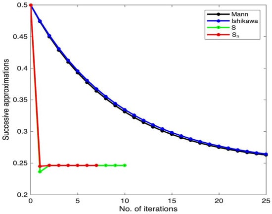
To justify the choice of the iterative process $S_n$, at the end of this section we will present a numerical simulation. First of all, we will mention that we considered the operator provided in Example 1 and chose $x_0=0.5$ as the initial point.

Figure 1 exhibits the results concerning the orbit of $x_0=0.5$ when considering the three-step iteration procedure $S_n$ as an alternative to the one-step iterative scheme of Mann or the two-step iterations Ishikawa and S. One can easily notice that the $S_n$ iteration provides a shorter orbit.

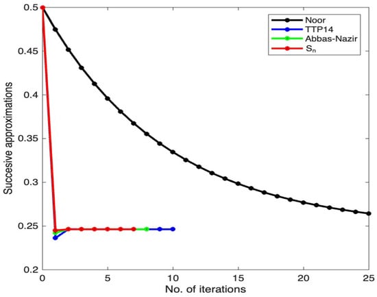
A similar result is presented in Figure 2, picturing a comparison between some three-step iterative processes, such as Noor, TTP14, Abbas–Nazir, and, of course, $S_n$. This time as well, a shorter orbit results from applying the $S_n$ procedure.

Finally,

Table 1. Output data.

Procedure	Number of Iterations	Numerical Solution
Mann	25	$0.262796752986884$
Ishikawa	25	$0.264377261799819$
S	10	$0.246266172167723$
Noor	25	$0.264331339777241$
TTP14	10	$0.246266172167723$
Abbas–Nazir	8	$0.246266172167723$
$S_n$	7	$0.246266172167723$

synthesizes the information resulting from running the Matlab program and contains the number of iterations performed (with the mention that the maximum number of steps was set to 25) and also the value of the estimated solution. We notice that the iterative process $S_n$ required the smallest number of steps (only 7 iterations were necessary) to reach the fixed point within a settled admissible error of ${10}^{-15}$.

As a general setting, we used the constant step-sizes $\alpha =0.1$ for the Mann iteration, $\alpha =0.1$ and $\beta =0.9$ for the Ishikawa and S procedures, $\alpha =0.1$ and $\beta =\gamma =0.9$ for Noor, TTP14, and $S_n$. It is worth mentioning that this choice of parametric values is not unique. The step-sizes act as control parameters, which can be adjusted according to needs, so that the efficiency of the studied procedures is improved. In fact, this motivates the advantages of using multi-step procedures, thus increasing the number of control elements and, consequently, the chances of obtaining the solution faster.

4. Local Maxima of Polynomial Modulus

In this section, we change the perspective and emphasize another possible use of the $S_n$ iteration procedure. Let p be a nonconstant polynomial, defined on the unit disk $D=\left\{z\in \mathbb{C}:\left|z\right|\le 1\right\}$. The maximum modulus principle states that the maximal value of the modulus, namely ${\displaystyle {∥p∥}_{\infty }=\underset{z\in D}{max}\left\{\left|p\left(z\right)\right|\right\}}$, is reached at points lying on the boundary of D. In [25], Kalantari marked an important step forward and advanced a new idea regarding the problem of maximizing the modulus of complex polynomials. More precisely, he initially rephrased the entire issue in terms of a fixed point problem and then in terms of a root search of some adequate pseudo-polynomial. This entire approach was enabled by the equivalence stated below.

Theorem 6

([25]). Let $p\left(z\right)$ be a nonconstant polynomial on $D=\left\{z\in \mathbb{C}:\left|z\right|\le 1\right\}$. A point $z_{*}\in D$ is a local maximum of $\left|p\left(z\right)\right|$ over D if and only if

$$z_{*}=F\left(z_{*}\right),$$

(41)

where $F\left(z\right)=\left({\displaystyle \frac{p\left(z\right)}{p^{\prime }\left(z\right)}}\right)/\left(|{\displaystyle \frac{p\left(z\right)}{p^{\prime }\left(z\right)}}|\right)$, meaning that it finds itself among the solutions of the zero-search problem

$$G\left(z_{*}\right)=0,$$

(42)

where $G\left(z\right)=p\left(z\right)|p^{\prime }\left(z\right)|-z{p}^{\prime }\left(z\right)\left|p\left(z\right)\right|$.

Due to its particular shape, the function G was called pseudo-polynomial. Anticipating the idea of using the Newton’s method to solve Equation (42), but also considering the nontrivial structure of G, Kalantari proposed a pseudo-Newton procedure that preserved the classical Newton-like pattern but altered the pseudo-polynomial G at each step, so as to bring it closer to conventional polynomials. The resulting procedure was

$$\left\{\begin{array}{c}{z}_1\in D\hfill \\ {\displaystyle z_{n+1}=z_n-\frac{G_n\left(z_n\right)}{G_n^{\prime }\left(z_n\right)},n=1,2,...,}\hfill \end{array}\right.$$

(43)

where $G_n$ is defined as

$$G_n\left(z\right)=p\left(z\right)|p^{\prime }\left(z_n\right)|-z{p}^{\prime }\left(z\right)\left|p\left(z_n\right)\right|.$$

(44)

Further on, the efficiency of the method was analyzed in [25], for several polynomials, by means of polynomiographs (2D colored images that emphasize through their color palette the length of the orbits through the given iterative construction, see also [26]).

It is easy to notice that the pseudo-Newton method (43) results from running a Picard-type iteration procedure for the pseudo-Newton iteration function ${\displaystyle N_n\left(z\right)=z-\frac{G_n\left(z\right)}{G_n^{\prime }\left(z\right)}}$. Kalantari suggested the possibility, which was further consistently approached by Gdawiec and Kotarski ([27]), of using other types of iteration functions, combined perhaps with more complex iterative schemes, to generate new pseudo-methods for solving the maximum modulus problem. The resulting procedures were called MMP methods. An important starting point on this topic is presented in [28].

In this section, we will couple the $S_n$ iteration procedure with some elements from the Basic Family of Iterations, adapted for the sequence of functions $\left\{G_n\left(z\right)\right\}$. More precisely, we will consider the first three elements of the Basic Family and their corresponding sequences of MMP iteration functions:

$$\begin{array}{ccc}(B_2 \mathrm{o}\mathrm{r} \mathrm{p}\mathrm{s}\mathrm{e}\mathrm{u}\mathrm{d}\mathrm{o}\text{-}\mathrm{N}\mathrm{e}\mathrm{w}\mathrm{t}\mathrm{o}\mathrm{n})\hfill & B_{2,n}\left(z\right)\hfill & {\displaystyle =N_n\left(z\right)=z-\frac{G_n\left(z\right)}{G_n^{\prime }\left(z\right)}}\hfill \\ \\ (B_3 \mathrm{o}\mathrm{r} \mathrm{p}\mathrm{s}\mathrm{e}\mathrm{u}\mathrm{d}\mathrm{o}\text{-}\mathrm{H}\mathrm{a}\mathrm{l}\mathrm{l}\mathrm{e}\mathrm{y})\hfill & B_{3,n}\left(z\right)\hfill & {\displaystyle =H_n\left(z\right)=z-\frac{2G_n^{\prime }\left(z\right)G_n\left(z\right)}{2G_n^{\prime }{\left(z\right)}^2-G_n^{\prime \prime }\left(z\right)G_n\left(z\right)}}\hfill \\ \\ \left(B_4\right)\hfill & B_{4,n}\left(z\right)\hfill & {\displaystyle =z-\frac{6G_n^{\prime }{\left(z\right)}^2{G}_n\left(z\right)-3G_n^{\prime \prime }\left(z\right)G_n{\left(z\right)}^2}{G_n^{\prime \prime \prime }\left(z\right)G_n{\left(z\right)}^2+6G_n^{\prime }{\left(z\right)}^3-6G_n^{\prime \prime }\left(z\right)G_n^{\prime }\left(z\right)G_n\left(z\right)}.}\hfill \end{array}$$

(45)

If $T_n$ indicates any of the MMP iteration functions listed above, then the resulting $S_n$-MMP procedure is

$$\left\{\begin{array}{c}{x}_{n+1}=\left(1-{\alpha }_n\right)T_n{z}_n+{\alpha }_n{T}_n{y}_n;\hfill \\ z_n=\left(1-{\gamma }_n\right)x_n+{\gamma }_n{y}_n;\hfill \\ y_n=\left(1-{\beta }_n\right)x_n+{\beta }_n{T}_n{x}_n,\hfill \end{array}\right.$$

(46)

for all $n\ge 1$, where $\left\{{\alpha }_n\right\}$, $\left\{{\beta }_n\right\}$ and $\left\{{\gamma }_n\right\}$ are real sequences in $\left[0,1\right]$.

Example 3.

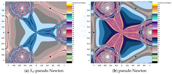
In the following, we apply the $S_n$-MMP procedures to find the maximum modulus of the complex polynomial $p\left(z\right)=z^3-1$. Alternatively, for comparison purposes, we will also use the classical MMP procedures, based on the Picard iteration. The initial data for the numerical algorithms requires entering the iteration step sizes (and we will use ${\displaystyle {\alpha }_n=\frac{1}{2}}$, ${\displaystyle {\beta }_n=\frac{1}{10}}$, and ${\displaystyle {\gamma }_n=\frac{9}{10}}$—this is an arbitrary choice, without any particular reasoning), as well as establishing the exit criteria. We use two such stopping elements: a maximal admissible error $\epsilon ={10}^{-5}$ and a maximal admissible number of iterations $K=31$. Hence, the iterative construction will stop when either two consecutive elements of the orbit are closed enough or the orbit has reached the length of 31 iterations. This will help us avoid having too long or too slow orbits, which fail to efficiently provide a solution of the problem.

The algorithmic procedure takes the points of a selected rectangle as initial estimates, generates their orbits, and assigns them a color, depending on the number of iterations that were performed.

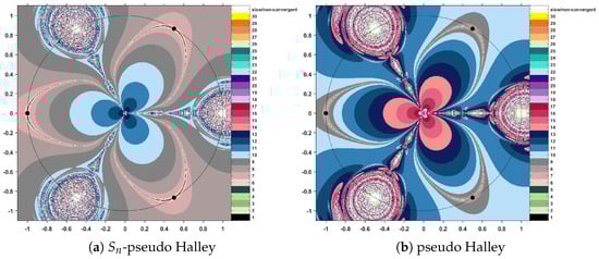
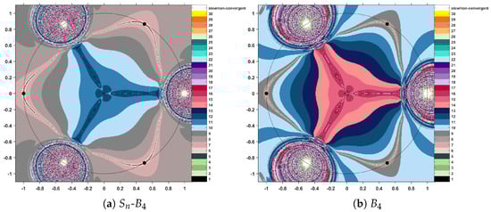
Comparing conventional MMP iterations with the corresponding methods modified through the $S_n$ scheme, we find that the modified procedures produce a decrease in the level of color intensity each time. Following these effects on the color map that accompanies the polynomiographic images, the effect is one of reducing the number of iterations necessary to reach a solution. This fact entitles us to state that the $S_n$ iteration applied to iterative methods speeds up the convergence of the orbits. More precisely, less intense colors indicate shorter orbits and hence a more efficient algorithm. The resulting polynomiographs are pictured in Figure 3, Figure 4 and Figure 5.

5. Conclusions

This study performed an analysis of Garcia-Falset operators in the setting of Banach spaces, based on a particular three-step iteration procedure. The main outcomes provided several weak and strong convergence results. Additionally, to emphasize the efficiency of the $S_n$ iteration procedure in practical nonlinear analysis, a numerical experiment related to the maximum modulus of complex polynomials was performed. The main instruments used were polynomialography, along with some of Kalantari’s pseudo-iteration functions, and the conclusion revealed a clear advantage of the S_n-MMP over the conventional MMP methods.

References

- Picard, E. Mémoire sur la théorie des équations aux dérivées partielles et la méthode des approximations successives. J. Math. Pure Appl. 1890, 6, 145–210. [Google Scholar]
- Garcia Falset, J.; Llorens Fuster, E.; Suzuki, T. Fixed point theory for a class of generalized nonexpansive mappings. J. Math. Anal. Appl. 2011, 375, 185–195. [Google Scholar] [CrossRef]
- Usurelu, G.I.; Bejenaru, A.; Postolache, M. Operators with property (E) as concerns numerical analysis and vizualization. Numer. Funct. Anal. Optim. 2020, 41, 1398–1419. [Google Scholar] [CrossRef]
- Suzuki, T. Fixed point theorems and convergence theorems for some generalized nonexpansive mappings. J. Math. Anal. Appl. 2008, 340, 1088–1095. [Google Scholar] [CrossRef]
- Karapinar, E. Remarks on Suzuki (C)-condition. In Dynamical Systems and Methods; Springer: New York, NY, USA, 2012. [Google Scholar]
- Pant, R.; Shukla, R. Approximating fixed points of generalized α-nonexpansive mappings in Banach spaces. Numer. Funct. Anal. Optim. 2017, 38, 248–266. [Google Scholar] [CrossRef]
- Pandey, R.; Pant, R.; Rakocevic, V.; Shukla, R. Approximating fixed points of a general class of nonexpansive mappings in Banach spaces with applications. Results Math. 2019, 74, 7. [Google Scholar] [CrossRef]
- Mann, W.R. Mean value methods in iteration. Proc. Am. Math. Soc. 1953, 4, 506–510. [Google Scholar] [CrossRef]
- Ishikawa, S. Fixed points by a new iteration method. Proc. Amer. Math. Soc. 1974, 44, 147–150. [Google Scholar] [CrossRef]
- Noor, M.A. New approximation schemes for general variational inequalities. J. Math. Anal. Appl. 2000, 251, 217–229. [Google Scholar] [CrossRef]
- Agarwal, R.P.; O’Regan, D.; Sahu, D.R. Iterative construction of fixed points of nearly asymptotically nonexpansive mappings. J. Nonlinear Convex Anal. 2007, 8, 61–79. [Google Scholar]
- Thakur, B.S.; Thakur, D.; Postolache, M. New iteration scheme for numerical reckoning fixed points of nonexpansive mappings. J. Inequal. Appl. 2014, 1, 328. [Google Scholar] [CrossRef]
- Abbas, M.; Nazir, T. A new faster iteration process applied to constrained minimization and feasibility problems. Mat. Vesn. 2014, 66, 223–234. [Google Scholar]
- Sintunavarat, W.; Pitea, A. On a new iteration scheme for numerical reckoning fixed points of Berinde mappings with convergence analysis. J. Nonlinear Sci. Appl. 2016, 9, 2553–2562. [Google Scholar] [CrossRef]
- Berinde, V. Picard iteration converges faster than Mann iteration for a class of quasi-contractive operators. Fixed Point Theory Appl. 2004, 2, 97–105. [Google Scholar] [CrossRef]
- Calineata, C.; Ciobanescu, C. Convergence theorems for operators with condition (E) in hyperbolic spaces. U. Politeh. Buch. Ser. A 2022, 84, 9–18. [Google Scholar]
- Ciobanescu, C.; Postolache, M. Nonspreading mappings on modular vector spaces. U. Politeh. Buch. Ser. A 2021, 83, 3–12. [Google Scholar]
- Bejenaru, A.; Ciobanescu, C. New partially projectiv algorithm for split feasibility problems with application to BVP. J. Nonlinear Convex Anal. 2022, 23, 485–500. [Google Scholar]
- Bejenaru, A.; Ciobanescu, C. Common fixed points of operators with property (E) in CAT(0) spaces. Mathematics 2022, 10, 433. [Google Scholar] [CrossRef]
- Goebel, K.; Kirk, W.A. Topic in Metric Fixed Point Theory; Cambridge University Press: Cambridge, UK, 1990. [Google Scholar]
- Opial, Z. Weak convergence of the sequence of succesive approximations for nonexpansive mappings. Bull. Am. Math. Soc. 1967, 73, 595–597. [Google Scholar] [CrossRef]
- Schu, J. Weak and strong convergence of fixed points of asymptotically nonexpansive mappings. Bull. Austral. Math. Soc. 1991, 43, 153–159. [Google Scholar] [CrossRef]
- Edelstein, M. Fixed point theorems in uniformly convex Banach spaces. Proc. Am. Math. Soc. 1974, 44, 369–374. [Google Scholar] [CrossRef][Green Version]
- Senter, H.F.; Dotson, W.G. Approximating fixed points of nonexpansive mappings. Proc. Am. Math. Soc. 1974, 44, 375–380. [Google Scholar] [CrossRef]
- Kalantari, B. A Necessary and Suffcient Condition for Local Maxima of Polynomial Modulus Over Unit Disc. arXiv 2016, arXiv:1605.00621. [Google Scholar]
- Kalantari, B. Polynomial Root-Finding and Polynomiography; World Scientific: Singapore, 2009. [Google Scholar]
- Gdawiec, K.; Kotarski, W. Polynomiography for the polynomial infinity norm via Kalantari’s formula and non-standard iterations. Appl. Math. Comput. 2017, 307, 17–30. [Google Scholar]
- Usurelu, G.I.; Bejenaru, A.; Postolache, M. Newton-like methods and polynomiographic visualization of modified Thakur processes. Int. J. Comput. Math. 2021, 98, 1049–1068. [Google Scholar] [CrossRef]
Disclaimer/Publisher’s Note: The statements, opinions and data contained in all publications are solely those of the individual author(s) and contributor(s) and not of MDPI and/or the editor(s). MDPI and/or the editor(s) disclaim responsibility for any injury to people or property resulting from any ideas, methods, instructions or products referred to in the content. |
© 2025 by the author. Licensee MDPI, Basel, Switzerland. This article is an open access article distributed under the terms and conditions of the Creative Commons Attribution (CC BY) license (https://creativecommons.org/licenses/by/4.0/).