Abstract
The COVID-19 pandemic was a profoundly influential global occurrence in recent history, impacting daily life, economics, and healthcare systems for an extended period. The abundance of data has been essential in creating models to simulate and forecast the dissemination of infectious illnesses, aiding governments and health organizations in making educated decisions. This research primarily focuses on designing a control technique that incorporates the five most important inputs that impact the spread of COVID-19 on the Romanian territory. Quantitative analysis and data filtering are two crucial aspects to consider when developing a mathematical model. In this study the transfer function principle was used as the most accurate method for modeling the system, based on its superior fit demonstrated in a previous study. For the control strategy, a PI (Proportional-Integral) controller was designed to meet the requirements of the intended behavior. Finally, it is showed that for such complex models, the chosen control strategy, combined with fine tuning, led to very accurate results.
Keywords:
COVID-19; SARS-CoV-2 virus; control design; prediction; pandemic dynamics; mathematical model; data processing; neural networks MSC:
93-10
1. Introduction
Five years since the outbreak of COVID-19, the repercussions continue to resonate strongly due to significant secondary health effects and the potential for future similar outbreaks. The COVID-19 pandemic, caused by the SARS-CoV-2 virus, started in December 2019 in Wuhan, China.
Initial reports traced many of the first cases to the Huanan Seafood Wholesale Market, which sold live wild animals. This suggested a zoonotic origin, with the virus transmitted from animals to humans. SARS-CoV-2 likely originated in bats, as it shares significant genetic similarities with bat coronaviruses, but the exact intermediate host remains undetermined [1].
One significant difference lies in transmissibility. While SARS had a case–fatality rate (CFR) of approximately 10%, among these three, it was the least transmissible due to the delayed onset of infectiousness. Similarly, MERS, with a higher CFR of around 35%, had limited human-to-human transmission, primarily within healthcare settings [2,3].
Zoonotic spillovers, where viruses cross species barriers, have caused several past outbreaks, including the SARS (2002) and MERS (2012) epidemics, which also involved coronaviruses [3].
Lockdowns, travel restrictions, and widespread testing became essential strategies for mitigating the virus’s spread. These interventions, while effective to varying degrees, were reminiscent of those used during the SARS epidemic in 2003, where quarantine and contact tracing successfully curtailed the outbreak [3]. The entry point of SARS-CoV-2’s into humans is believed to have occurred through natural mechanisms, as its spike protein binds efficiently to human ACE2 receptors, facilitating infection [4].
The virus’s high reproduction number (R0) and its ability to transmit via asymptomatic carriers were critical factors in its wide spread. This ability contrasts with SARS, where transmission started primarily from symptomatic individuals, making containment more feasible [5]. Within weeks of the outbreak, SARS-CoV-2 spread beyond China, reaching multiple continents. Human-to-human transmission was initially confirmed in healthcare settings, as frontline workers were among the earliest clusters of secondary cases [5]. A Public Health Emergency of International Concern (PHEIC) was declared by the World Health Organization (WHO) on 30 January 2020, and a pandemic was announced on 11 March 2020 [6]. Both of these declarations were made by the WHO [6].
COVID-19 shares significant biological and epidemiological similarities with other zoonotic viral diseases. SARS-CoV-2, along with SARS-CoV and MERS-CoV, is a member of the beta coronavirus genus. It is distinguished by its spike protein, which is recognized for its significant contribution to the process of entering host cells. These viruses primarily affect the respiratory system and can cause severe acute respiratory distress in critical cases [6].
Unlike its predecessors, SARS-CoV and MERS-CoV, which had limited transmission due to localized outbreaks and strict containment measures, SARS-CoV-2 exhibited high transmissibility, which allowed its rapid global spread [7].
The recurring emergence of zoonotic viruses, such as SARS-CoV-2, highlights the need for better global surveillance and response systems. The COVID-19 pandemic revealed significant global gaps in preparedness despite the past outbreaks’ alarming lessons. For example, investments in vaccine platforms during the SARS epidemic facilitated the rapid development of COVID-19 vaccines, but similar investments in diagnostic and therapeutic tools were lacking [7]. The COVID-19 pandemic has profoundly impacted Europe, affecting public health, economies, and societies at large.
Moreover, SARS-CoV-2 displayed a unique mix of high transmissibility and moderate CFR, making it very difficult to suppress [8].
On 11 March 2020, the World Health Organization (WHO) declared COVID-19 a pandemic. Europe quickly became a hotspot, with countries like Italy and Spain experiencing significant outbreaks early on. The European Region has since reported over 2.3 million deaths related to COVID-19, underscoring the virus’s severe impact on the continent [9].
European nations implemented a variety of public health measures to curb the virus’s spread. These included lockdowns, social distancing mandates, mask requirements, and travel restrictions. The European Commission played a pivotal role in coordinating these efforts, securing up to 4.2 billion vaccine doses for EU citizens and supporting non-EU countries [10]. By 2021, over 80% of the EU population had been fully vaccinated, reflecting the success of these initiatives.
The pandemic’s economic repercussions were heterogeneous across the Euro area. Factors such as the stringency of containment measures, sectoral compositions, and financial capacities influenced the degree of economic contraction experienced by different countries. The European Central Bank highlighted these disparities, noting that countries with larger service sectors, particularly tourism, faced more substantial declines in economic activity [11].
Despite concerted efforts, the pandemic exposed several challenges in policy implementation. A study exploring EU country responses found that scientists advising policymakers grappled with high uncertainty and risks in an environment filled with unknowns. This situation underscored the need for robust evidence to determine which measures were effective in responding to the pandemic [12].
In response to the economic downturn, European governments introduced various fiscal measures to support businesses and individuals. The International Monetary Fund (IMF) documented these efforts, noting that the total budget cost of spending measures in certain countries amounted to significant portions of their GDPs. These measures aimed to mitigate the pandemic’s adverse effects on employment and economic stability [13]. Accurate data collection and surveillance were critical in managing the pandemic. The United Nations Statistics Division conducted surveys to assess the impact of COVID-19 on demographic and social statistics, highlighting the importance of reliable data in shaping effective public health responses [14].
The COVID-19 pandemic reached Romania on 26 February 2020, when the first confirmed case was reported. The patient was a man who had come into contact with an Italian citizen, later tested positive for the virus. By May 26, 2020, Romania had reported 18,429 confirmed cases of COVID-19, with 11,874 recoveries and 1210 deaths [15].
The government took stringent precautions during this time period, including the implementation of lockdowns, social separation, mask regulations, and the shutdown of companies that were not critical to normal operations. Additionally, movement between cities was restricted, and international travel was heavily regulated to prevent imported cases [15]. These figures reflected the pandemic initial impact on the country, highlighting the virus’s rapid spread and its burden on public health infrastructure. Romania declared a state of emergency on 16 March 2020 to curb the virus’s spread. This lasted until 14 May 2020, when it transitioned to a state of alert, a less restrictive phase that allowed for some economic activities to resume [16].
Despite these efforts, Romania experienced two major waves of infections in 2020, one during the initial spring outbreak and another in late autumn. The healthcare system faced considerable challenges, partly due to its limited capacity.
In 2019, Romania allocated only 5.7% of its GDP to healthcare, the second-lowest expenditure among European Union countries [17]. Hospitals were strained, with intensive care units (ICUs) operating near capacity during peak periods of infection [18].
The pandemic exposed vulnerabilities in Romania’s healthcare system and social infrastructure. Romania’s reliance on transnational labor played a significant role in the virus’s spread. It was during the early phases of the epidemic when a significant number of Romanians who had been working abroad, especially Italy, came home, bringing the virus along with them [19]. This movement highlighted the interconnectedness of labor migration and public health in Romania.
Romania’s COVID-19 experience mirrored global trends in several respects. The initial response involved strict lockdowns, similar to those implemented in other European countries like Italy and Spain [20]. However, the strain on the healthcare system in Romania was particularly acute due to underfunding and limited resource, as healthcare expenditure in Romania is the lowest in the EU, a one third of the EU average [21].
Despite these difficulties, Romania demonstrated resilience by leveraging international support and focusing on the rapid acquisition of medical supplies and equipment.
The findings of research collectively indicate the importance of integrating preventative measures, predictive modeling, and early treatments in order to effectively control the spread of COVID-19 across the population. As public health interventions reduce the transmission of disease, predictive models assist in making decisions regarding resource allocation, and therapeutic techniques hold promise for the management of pandemics in the future. The virus’s rapid global spread resulted in significant morbidity and mortality, prompting unprecedented public health responses worldwide.
Understanding the origins and early transmission dynamics of COVID-19 is crucial for preventing future pandemics and improving global health responses.
COVID-19 remains a circulating virus with periodic surges, often linked to seasonal changes and emerging variants. While overall severe cases have decreased due to widespread immunity, vulnerable populations (elderly, immunocompromised) still face higher risks.
Experts predict that COVID-19 will continue to circulate seasonally, potentially requiring regular vaccine updates. Long-term surveillance will focus on tracking variants, monitoring immunity levels, and refining treatment options. The risk of new pandemics emerging from similar coronaviruses remains, reinforcing the need for global preparedness.
Through the use of modeling and simulation, the fundamental objective of this study is to establish a joined strategy for preventing the spread of the SARS-CoV-2 virus across the Romanian territory. This objective is driven by the current lack of a comprehensive solution capable of predicting the evolution of key pandemic-related parameters, including the state of the healthcare system, in relation to both time and geographic distribution.
Recent advances in epidemic modeling have explored the incorporation of stochastic dynamics, delays, and jump disturbances into classical compartmental frameworks such as the SIR model. For example, in [22], a finite-time stability analysis of a stochastic SIR system influenced by Lévy noise and time-delay effects is proposed. In this formulation, random fluctuations and abrupt epidemic shocks are modeled using Brownian motion and Lévy processes, enabling a more realistic representation of transmission variability, such as super-spreader events or sudden policy shifts. Control inputs, such as vaccination or intervention measures, are embedded in the model and analyzed using Lyapunov-based methods to ensure that infections remain bounded and decay within a predefined time horizon. While this approach captures the nonlinear and stochastic nature of disease spread, it often requires strong mathematical assumptions and is analytically complex [22].
Another study presents a COVID-19 transmission model using fractional-order differential equations to incorporate memory effects in disease dynamics. The model includes six population compartments—such as susceptible, exposed, and hospitalized—allowing for realistic tracking of disease progression. It accounts for partial vaccine protection and waning immunity, reflecting real-world conditions where vaccines are not always fully effective. Using Caputo fractional derivatives, the model better captures the historical dependence of infection rates. Numerical simulations show that vaccination failure significantly influences the outbreak’s duration and severity.
A key aspect of the modeling approach is the use of Caputo fractional derivatives, which introduce memory effects into the system. This allows the model to reflect real-world dynamics more accurately, where the present rate of change in infection may depend not only on current conditions but also on historical patterns of transmission and immunity. The fractional order, varying between 0 and 1, governs the strength of this memory. Through calibration, the authors found that a value of approximately 0.86 provided the best fit to real-world data [23].
A different approach is detailed in [24], offering a mathematically rigorous and clinically relevant framework by combining advanced mathematical tools with biological realism to model individual-level immune responses to COVID-19. The use of fractional-order differential equations, particularly those involving the Caputo derivative, adds depth to the model by accounting for memory-dependent dynamics. Unlike traditional models that only consider current rates of change, fractional models allow for past states to influence present immune behavior. This is especially crucial in COVID-19, where immune response patterns like delayed activation, prolonged inflammation, and long COVID cannot be accurately captured by classical methods.
Clinically, the model is calibrated and validated using real patient data, showing strong agreement with observed immune trajectories. This makes the model not only theoretical but also practically applicable for interpreting patient-level outcomes. Moreover, the sensitivity analysis pinpoints which biological parameters have the most influence on infection outcomes, which can help guide therapeutic strategies, such as optimizing antiviral treatment timing or enhancing vaccine design [24].
By integrating mathematical precision with clinical observations, the model serves as a powerful tool for predicting and understanding the immune kinetics of COVID-19 at the individual level, including challenging scenarios like prolonged infection and immune system fatigue. It bridges the gap between abstract modeling and patient-specific insights—an essential step toward personalized medicine in infectious disease management [24].
Additionally, the absence of effective methodologies for pandemic control highlights the importance of this research. By creating and simulating a mathematical model of virus transmission, this study seeks to facilitate detailed analyses of the pandemic’s impact on Romanian society and inform strategies for its control, in case of future similar situations.
The proposed work focuses on creating a mathematical model to understand and control the spread of SARS-CoV-2, which is critical in devising effective public health strategies. The goal is to predict how various factors—such as human behavior, mobility, intervention measures, and environmental influences—affect the pandemic’s dynamics and use this knowledge to inform decisions that limit virus transmission.
By implementing this, the authorities can make informed decisions that balance public health and socio-economic considerations, which will provide the following advantages:
- Localized solutions: tailored interventions based on regional dynamics.
- Predictive power: anticipating future outbreaks and healthcare needs.
- Flexibility: adapting strategies in real time as conditions evolve.
- Comprehensive analysis: incorporating multiple inputs and outputs for holistic understanding.
The first chapter serves as an introduction, providing an overview of the study and establishing the foundation for the analysis.
The second chapter focuses on presenting the gathered data used for model identification, along with a detailed description of the mathematical modeling of the system. The input signals that were utilized in the modeling process are discussed, and the influence that these signals had on the propagation of the COVID-19 virus is investigated.
Also, it addresses on the control design techniques applied to the mathematical model of the pandemic. Here, the methodologies employed are discussed, together with their underlying principles, and their effectiveness in managing the dynamics of the system is evaluated.
A simulation of the proposed model is carried out in the fourth chapter, and the control simulations that are produced as a result are explained and interpreted. The analysis of the results is also presented in this chapter, which demonstrates the validity of the model and its capacity to forecast future developments in the pandemic.
In conclusion, the final chapter provides a summary of the findings as well as insights into prospective future study avenues that could be pursued in this particular field.
2. Design and Implementation
Among the sources from which the essential dataset for model identification was collected are infectious disease hospitals and specialized research institutions. These sources are among the authoritative sources that are actively engaged in the management of the Romanian pandemic.
This dataset, covering the period from 28 February 2020 to 30 September 2020, was meticulously gathered on a daily basis from each county in Romania and methodically archived in a specialized database.
Following the establishment of the database, the data was analyzed through a number of processing procedures in order to derive the mathematical model of the dynamics of the pandemic in Romania, as demonstrated in the following paragraphs:
- Data Verification and Completion: the dataset was examined to ensure continuity, verifying that no days or information was missing. Any identified gaps were addressed by collecting the missing data to create a complete and accurate database.
- Daily Data Aggregation: the data were processed each day to derive relevant national-level information. For instance, data from all counties were aggregated, with certain parameters like temperature or humidity being averaged arithmetically to represent countrywide conditions.
- Consistency Check: inconsistent entries within the dataset were identified and rectified. A detailed analysis was conducted to replace such discrepancies with reliable and verified information, ensuring consistency in the database.
- Data Organization: the refined data were then organized for subsequent analysis. This involved extracting and structuring the information into vector or matrix formats to facilitate further processing and modeling.
Following these processing steps, the dataset was categorized into two main groups:
- Inputs for Each Date: these included variables such as the number of tests conducted, indoor temperature (in enclosed spaces like supermarkets, offices, and rooms), outdoor temperature, outdoor humidity, and quantified indicators of measures implemented by authorities to mitigate the spread of COVID-19.
- Outputs for Each Date: how many new cases, how many deaths, how many cumulative cases, and how many total fatalities there have been.
This structured and processed dataset provided the foundational basis for constructing a robust mathematical model of the pandemic’s progression and understanding the impact of various factors on its dynamics.
The fast global propagation of COVID-19 necessitates the creation of precise and interpretable forecasting models to guide public health measures.
Among the different modeling approaches, control systems theory, specifically the Multiple-Input Single-Output (MISO) structure, provides a systematic and analytically accessible way to understanding the dynamic relationship between various influencing variables and major epidemiological outcomes.
A MISO system depicts the development of a single output variable, such as the daily number of new COVID-19 cases, as a function of many input variables, which may include behavioral, environmental, and policy-related factors.
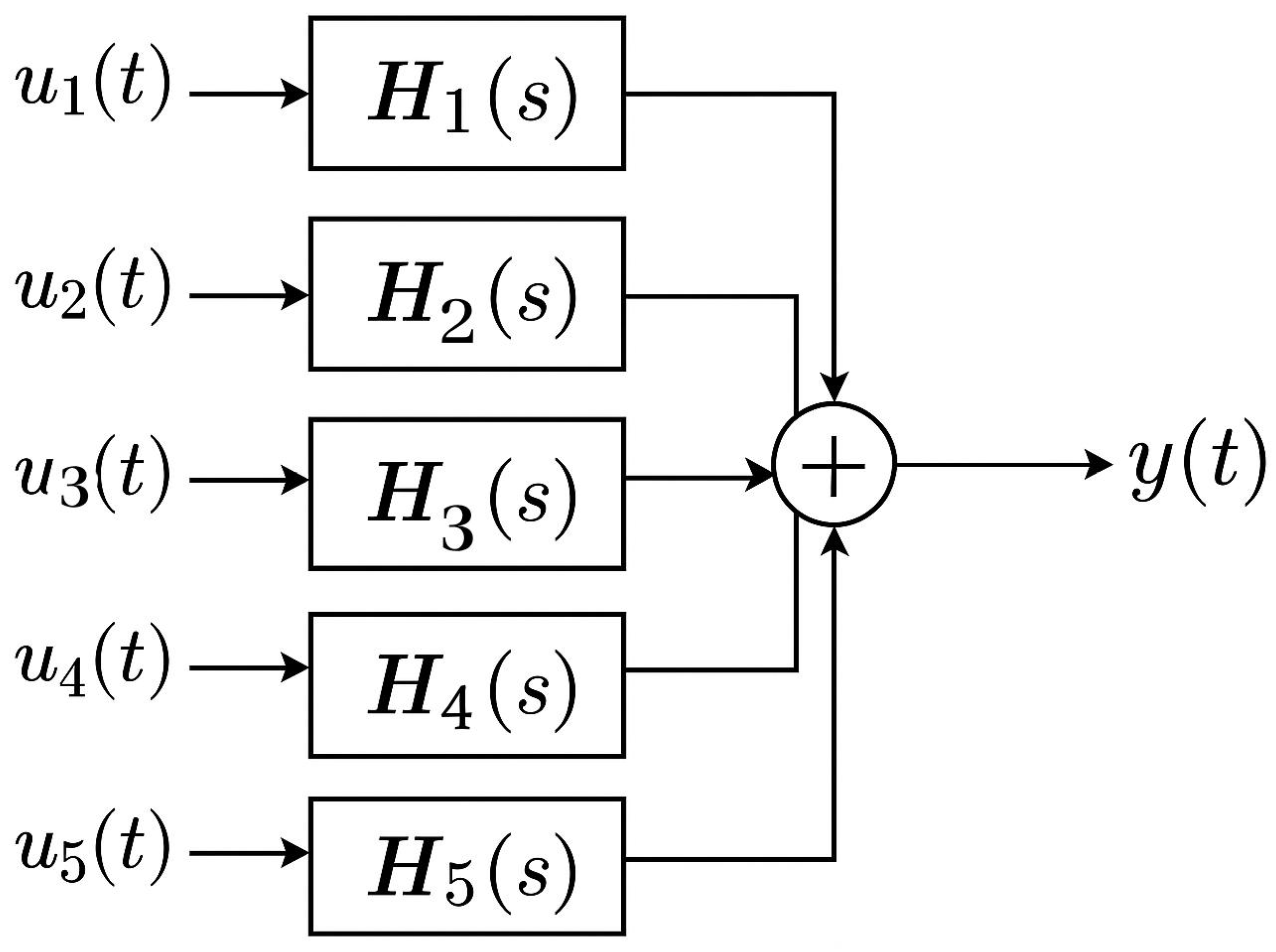
In this sense, the following MISO (Multiple-Input Single-Output) system was designed to incorporate the presented inputs and to obtain at the end the proposed output (Figure 1):
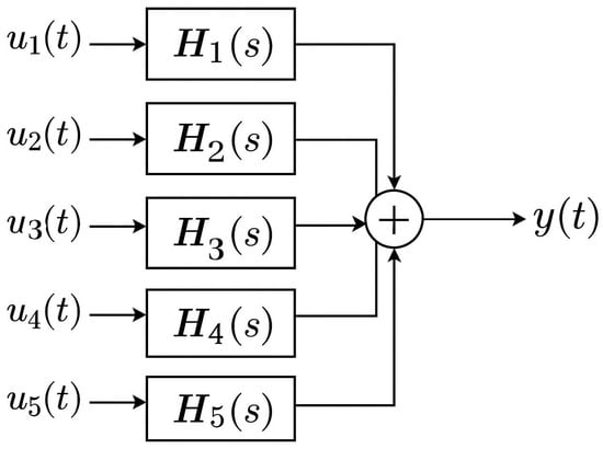
Figure 1.
MISO system diagram.
In the above diagram, the main components of a MISO model are highlighted, in this case, five inputs and one output.
In the MISO representation, each input is processed through a corresponding linear time-invariant (LTI) system characterized by its transfer function , which defines the dynamic response of the system to that input, where i =. The resulting system’s output, y(t) is the sum of the individual responses.
Although the spread of infectious diseases like COVID-19 is governed by inherently nonlinear dynamics, particularly as described by compartmental models (e.g., SEIR), LTI models such as the MISO structure can serve as useful approximations under specific conditions.
In this context, the MISO LTI structure enables the decomposition of the influence of multiple exogenous inputs—such as number of taken tests, policy interventions, and environmental conditions—on a single measurable output (daily case counts). Each input is assumed to contribute linearly and independently to the output via a corresponding transfer function. This approach is particularly useful for system identification from real-world data, where full mechanistic modeling is often infeasible due to incomplete knowledge of all transmission pathways and feedback loops.
Furthermore, LTI systems offer a well-established mathematical foundation for analyzing dynamic responses, including delays and frequency-dependent behaviors, which are commonly observed in epidemiological data. While the underlying disease dynamics are nonlinear, the LTI MISO model can still capture first-order effects and temporal correlations, making it a practical choice for forecasting and policy evaluation within constrained modeling horizons.
The COVID-19 pandemic has prompted a global investigation into the factors that influence the virus’s spread. Among these factors, environmental conditions such as temperature and humidity, indoor climate factors, and public health measures implemented by authorities have been identified as playing critical roles in the dynamics of COVID-19 transmission.
Temperature and humidity are known to affect the stability and spread of respiratory viruses, including SARS-CoV-2. Research has shown that SARS-CoV-2 transmission tends to be lower in warmer temperatures and higher humidity levels.
A study revealed that higher temperatures above 11 °C, coupled with high specific humidity, reduce the virus’s transmissibility by decreasing the stability of viral particles in the air, potentially decreasing their ability to infect individuals [22]. Similarly, another study noted that temperature inversely correlates with transmission rates, suggesting that cold, dry environments provide more favorable conditions for viral survival and transmission [25].
In contrast, high temperatures above 30 °C seem to reduce viral stability in aerosols and on surfaces, making the virus less transmissible. However, the global influence of temperature and humidity is not uniform, and its effect may vary across different regions and seasons. For example, a study indicated that tropical climates with higher temperatures and humidity levels might experience slower spread of the virus compared to temperate climates where the virus thrives in colder conditions [26].
However, this relationship is complex. A study found that while high temperature and humidity are important variables that can decrease the airborne stability of SARS-CoV-2, they are not sufficient on their own to stop the transmission of the virus in places with a high population density or in situations where public health interventions are inadequate [27]. Thus, while environmental factors like temperature and humidity influence virus spread, they are not the only determinants.
Indoor climate, particularly temperature and humidity levels in enclosed spaces, plays a crucial role in the transmission of this disease. The virus can remain viable in aerosols for extended periods, especially in poorly ventilated indoor spaces, where temperature and humidity levels are crucial. For instance, a research showed that maintaining appropriate indoor humidity levels can help reduce aerosol-based transmission by limiting the persistence of airborne virus particles [28].
In addition, interiors with increased air circulation and ventilation reduce the air concentration of virus particles, which in turn reduces the likelihood of transmission among individuals. In this context, understanding the ideal indoor temperature and humidity conditions can be key to reducing COVID-19 transmission in public and private settings.
Studies have demonstrated that SARS-CoV-2 remains viable in indoor air for several hours, with certain conditions such as cooler temperatures contributing to longer survival times for the virus [29]. Public health measures that have been implemented by governments have proven to be the most significant elements in reducing the spread of COVID-19. This is despite the fact that environmental factors such as temperature and humidity might have an impact on transmission. Measures such as mask-wearing, physical distancing, quarantine, and lockdowns have been essential in mitigating transmission.
A systematic review and meta-analysis highlighted that the use of face masks significantly reduced the incidence of COVID-19 in various settings, especially when combined with social distancing measures [30].
In line with this, one research suggested that strict lockdown measures, such as stay-at-home orders and social distancing, have been effective in curbing the virus’s spread, with countries implementing early lockdowns showing significantly fewer cases than those with delayed or no restrictions [31].
Similarly, studies showed that mass quarantines, restrictions on mass gatherings, and other public health interventions resulted in a decline in infection rates, mainly when implemented early in the pandemic. This was particularly evident in countries that had implemented robust testing and contact tracing systems alongside social distancing measures [32].
In terms of controlling transmission in specific sectors, government-mandated measures in workplaces, schools, and public transport have been influential. For example, a research found that enhanced hygiene protocols and mask mandates in schools significantly reduced the transmission rate among students and staff. While both environmental factors (such as temperature and humidity) and public health measures (such as mask-wearing and lockdowns) independently influence the transmission of COVID-19, the combination of these factors leads to a more complete understanding of how the virus spreads.
Another study emphasized that the effectiveness of public health measures is enhanced when environmental conditions are favorable.
However, the study also cautioned that extreme weather conditions, such as winter in temperate regions, might undermine the measures’ effectiveness, requiring enhanced strategies to ensure a controllable virus spread in colder months [33].
Another study analyzed the relationship between meteorological factors (temperature, humidity, and solar radiation) and COVID-19 incidence across 439 cities in 22 countries from February 2020 to August 2022.
Lower temperatures (approx.°C) were associated with a 1.22-fold increase in COVID-19 incidence compared to a reference temperature of 17 °C. Higher temperatures correlated with reduced virus transmission, likely due to faster viral inactivation in warmer conditions. Absolute humidity (total water vapor in the air) showed an inverse relationship with COVID-19 cases: lower humidity levels led to increased transmission.
Relative humidity (percentage of moisture in the air) did not have a significant impact on COVID-19 spread. As population immunity (from vaccines or past infections) increased over time, the effect of weather conditions on COVID-19 transmission weakened. In the early stages of the pandemic, meteorological factors had a stronger influence on case numbers.
In other words, cold and dry conditions favor COVID-19 spread, similar to other respiratory viruses. While weather still plays a role, population immunity and public health measures now have a greater impact on transmission dynamics [34].
While temperature, humidity, and indoor climate conditions certainly influence the transmission of COVID-19, the most significant impact on the spread of the virus arises from public health measures.
The countries that were proactive in implementing mask mandates, physical distancing policies, and lockdown measures were able to reduce the spread of COVID-19, regardless of the environmental conditions. Therefore, the coordinated public health efforts clearly play a more crucial role in controlling the pandemic, while environmental factors may affect the virus’s stability and transmission.
For this research, both the input and output data were processed in relation to time; specifically, the first 120 days were used for training the mathematical model, and the prediction was made for the next 60 days.
The following are some examples of data, both input and output, that were collected from the database that was used to make the predictions. These examples are provided in Table 1 and Table 2:

Table 1.
Instances of input records.

Table 2.
Instances of output records.
A system may be represented mathematically by a collection of equations that, with different degrees of accuracy or approximation, describe the behavior of the system. Each system may often be represented by a mathematical model that reflects its unique properties.
The structure and characteristics of this model can vary widely amongst systems, allowing for different representations of the same system. Each representation may highlight different characteristics or approximations of the system’s dynamics, resulting in various mathematical formulations.
In control theory, transfer functions are mathematical tools commonly used to describe the input–output relationship of linear time-invariant (LTI) systems in the frequency or Laplace domain, under the assumption of zero initial conditions.
Ordinary differential equations with coefficients that are constant are able to provide a time-based description of these systems.
Equation (1) describes the input-output relationship of a Single-Input Single-Output (SISO) system in the complex domain.
In this context, symbols Y(s), U(s), and E(s) are used to indicate the Laplace transforms of the input, output, and noise signals, respectively. Also, num(s) is the numerator polynomial, and den(s) is the denominator polynomial of the transfer function.
An equation describing a linear time-invariant system [35] is the differential equation that is shown below (2)
where y(t) represents the signal that is produced by the system, and x(t) represents the signal that is taken in by the system.
The coefficients and in Equation (2) are constant. Therefore, the differential equation that was stated in (1) can be utilized for the purpose of describing the operation of a linear system and its functioning.
This particular type of differential equation can be utilized for the purpose of modeling a SISO system. This is because (1) only has a single input signal and a single output signal (both of which are singular).
Utilizing Laplace transform with zero starting conditions to (1) yields (3)
where the Laplace transforms of the output signal, and the Laplace transforms of the input signal, , are represented. In addition, the transfer function of the system that is being modeled is denoted by the symbol H(s).
A system is only considered nearly viable if the value of n is greater than or equal to the value of m.
A system is deemed to be rigorously appropriate if the value of n is bigger than the value of m. This is the situation for the vast majority of systems that are realistically feasible. On the other hand, if n is equal to m, the system is considered to be proper.
The Laplace transform is advantageous for a number of reasons, the most important of which is that it transforms the differential Equation (2) into an arithmetical relation (in the complex domain), which is a considerably easier issue that can be solved mathematically.
In the context of COVID-19 prediction models, transitioning from SISO to MIMO and then to MISO illustrates how model complexity evolves to improve accuracy. A basic SISO (Single-Input Single-Output) model might predict the daily number of COVID-19 cases using a single input, such as mobility data. While this approach is simple, it cannot capture the full dynamics of virus spread, especially when multiple factors influence transmission rates.
To address this, models evolved into MIMO systems. These incorporate various inputs—mobility trends, testing rates, mask usage, weather, and government interventions—and predict multiple outputs simultaneously, such as new cases, hospitalizations, and deaths across multiple regions. This structure reflects the interconnected nature of pandemic dynamics and allows for more robust forecasting across variables.
However, when the focus narrows to forecasting a single critical output, like the daily number of new cases, the model is often reduced to a MISO form. In this case, multiple relevant inputs still influence the prediction, but only one output is modeled. This transition balances complexity and clarity, improving predictive performance while focusing on the most actionable outcome for public health decision-making.
The biological mechanism under investigation for SARS-CoV-2 spread changing aspects is known as MIMO. This is due to the fact that it is both complex, and there are a large number of factors that influence it.
SARS-CoV-2 spread, on the other hand, is described as a series of MISO models. This is performed to increase the correctness of the mathematical models that have been presented.
To be more exact, building a single mathematical model is the initial stage in estimating the total impact of all input signals on each output signal [36].
The standard linear differential equation for a MISO system with five inputs and a single output signal is given by Equation (4)
where the output signal is denoted by y(t), whereas the input signals are denoted by , , , , and , respectively.
To make the system feasible, the prerequisites , , and have to be concurrently accomplished.
For starting conditions of zero, the following equation is obtained by using the Laplace transform (5):
As a consequence of Equation (5), the output signal expression is as follows:
In (6), the following notations are made:
Based on Equations (7)–(11), the following form of Equation (6) is obtained:
The next five equations expressed in terms of zeros and poles were determined and are described in Table 3 as follows:

Table 3.
Transfer function representation in terms of poles and zeros.
For the following reasons, the transfer functions are essential: the transfer function is a correlation between the temperatures inside the building and the number of new COVID-19 cases; is a transfer function that was developed to correlate the quantity of new cases with the outside temperatures; a transfer function that correlates humidity with the amount of new cases is denoted by ; a transfer function that correlates the number of taken tests with the amount of new cases is represented by , and is concerned with the correlation between the quantitative rates of the COVID-19 measurements and the number of new occurrences.
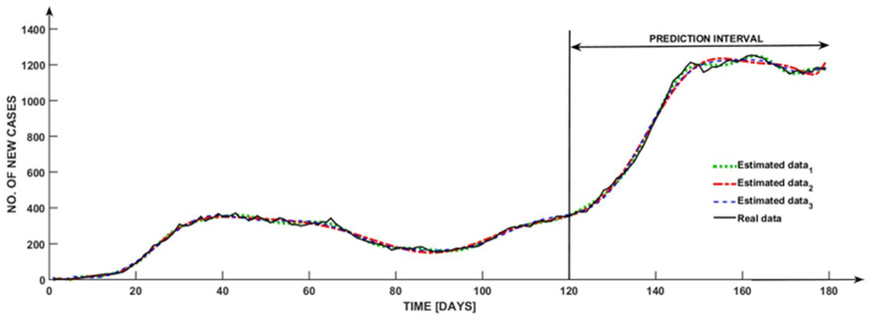
A black curve is shown in Figure 2, illustrating the progression of the amount of new cases that were “experimentally established” throughout the course of time.
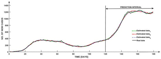
Figure 2.
Transfer functions estimation.
The remaining five colored curves are a representation of the graphical responses that the suggested model provides. These curves are determined via the use of continuous transfer functions, and they incorporate the input “experimental values”.
Concerning this particular instance, numerous adjustments were made to the amount of poles and zeros in order to achieve the best possible match. This was performed in order to carry out a comprehensive analysis of the most effective approach.
According to the illustration that follows, the predicted curves are very similar to the black curve, which represents the actual data curve. In addition, the obtained graphs outline the progression of the number of occurrences over a period of one hundred and twenty days.
The prediction that is provided by the continuous transfer vector model (although, this model does compromise the transfer functions , , , , and ) is that the interval that follows will be between [121 and 180] days.
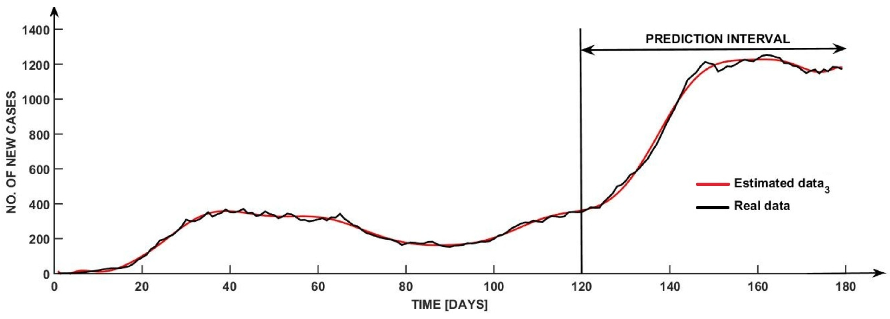
With a fit of 97.23%, the best solution is depicted in Figure 3, which was obtained by using Estimated data 3 from Table 4.
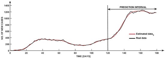
Figure 3.
Model-predicted vs. actual observed COVID-19 daily new cases over a 180-day period.

Table 4.
The parameters linked to continuous transfer functions.
Root Mean Squared Error (RMSE) is the metric used to evaluate the performance of prediction models by measuring the average magnitude of the errors between predicted values and actual values. It is described in (13)
where n is the number of data points, is the actual value for the observation, and is the predicted value for the observation.
An irregularity in data collection as a result of inadequate input supplied via public authorized platforms on weekends is the source of the variance in achieving a 100% fit. This irregularity influences the validation model, as was proved between days 135 and 160. Due to the fact that the estimated model does not exhibit any oscillations throughout this time period, the graph depicts a few oscillations; therefore, this may be an inevitable outcome of the inconsistency that was explained before.
Control design techniques are fundamental in engineering for developing systems that operate efficiently, reliably, and safely. The primary goal of control design is to regulate system behavior, ensuring that the output meets the desired performance criteria, even in the presence of uncertainties and disturbances.
One of the most common control design techniques is Proportional-Integral-Derivative (PID) control. PID controllers are widely used due to their simplicity and effectiveness in handling many engineering applications.
The proportional term reacts to the present error, the integral term accounts for past errors, and the derivative term predicts future errors to improve system stability and responsiveness.
One can fine-tune PID parameters to optimize performance, balancing speed, accuracy, and stability. While PID controllers work well for linear systems, they may require advanced tuning methods for more complex nonlinear systems.
Another important technique is state-space control, which provides a more comprehensive way to model and control dynamic systems.
Unlike traditional transfer function methods, state-space representation describes systems using a set of first-order differential equations, capturing multiple inputs and outputs in a compact form.
Techniques like pole placement and optimal control methods, such as Linear Quadratic Regulator (LQR), are used to design controllers that minimize energy consumption and improve system efficiency.
Adaptive and robust control techniques are designed to handle systems with uncertainties and time-varying parameters. Adaptive control continuously adjusts its parameters in real time based on system behavior, making it suitable for applications like aircraft flight control and robotic arms that experience changing conditions.
Robust control, such as H-infinity (H∞) control, ensures stability and performance even when the system is subject to disturbances or modeling inaccuracies. These techniques are essential in safety-critical applications where high reliability is required.
With the rise of artificial intelligence and machine learning, intelligent control techniques are becoming increasingly popular.
Neural networks, fuzzy logic, and reinforcement learning are now being integrated into control systems to improve decision-making and adaptability. These methods are particularly useful for nonlinear and highly complex systems where traditional control methods may struggle.
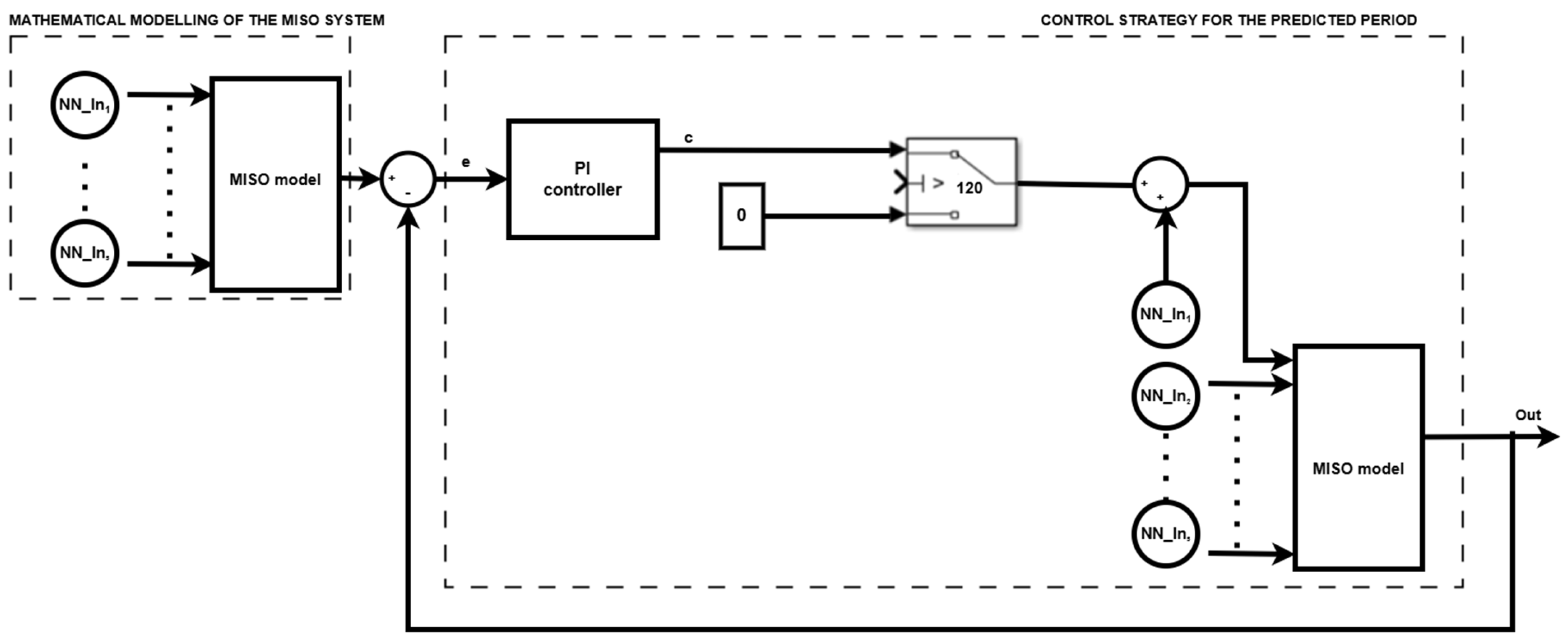
In this sense, for the presented mathematical model, a control strategy has been designed and is depicted in the following schematic (Figure 4).
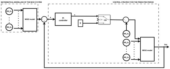
Figure 4.
Control design diagram.
This block diagram illustrates a predictive control system designed to manage the spread of COVID-19 using a MISO system. The system leverages a neural network-based model alongside a Proportional-Integral (PI) controller to make informed public health decisions.
The mathematical modeling section uses five key input variables: the number of tests conducted, indoor temperature, outdoor temperature, outdoor humidity, and quantified indicators of government-imposed mitigation measures (such as lockdowns, mask mandates, or social distancing rules).
In this sense, a FFNN (feed-forward neural network) was used for each of the five inputs, and the obtained five outputs were used further in the mathematical modeling: , , , , .
These inputs are processed by a trained MISO model to predict a single critical output—such as the number of new COVID-19 cases.
Out represents the output of the system, in this case, the total number of COVID-19 cases reported every day. This predicted output is compared with a target value (an acceptable threshold of daily cases), and the difference is calculated as the error (e).
This error is sent to the PI controller, which generates a control signal (c) representing the recommended adjustment in mitigation intensity. The conditional block is used as follows: the control signal is applied just after 120 days, so in this sense, the control is imposed at a certain time.
The control signal is then used to scale the inputs for the next prediction cycle. This updated data is reprocessed by the MISO model, and the output is fed back, forming a closed-loop system for dynamic COVID-19 response.
The reference was chosen so that the dynamics of the pandemic would stabilize (the number of cases would stop increasing).
The usefulness of this procedure lies in the fact that after stabilization, by adopting an additional measure, the dynamics of the pandemic could be forced to enter a downward slope.
In the case of pandemic-associated signals, the initial conditions were 0. In the case of neural networks used in learning the dynamics of input signals, the initial values of the weights were randomly initialized to small, but non-zero values.
The solution parameters of the neural networks were determined by training them, using the Levenberg–Marquardt learning method [37].
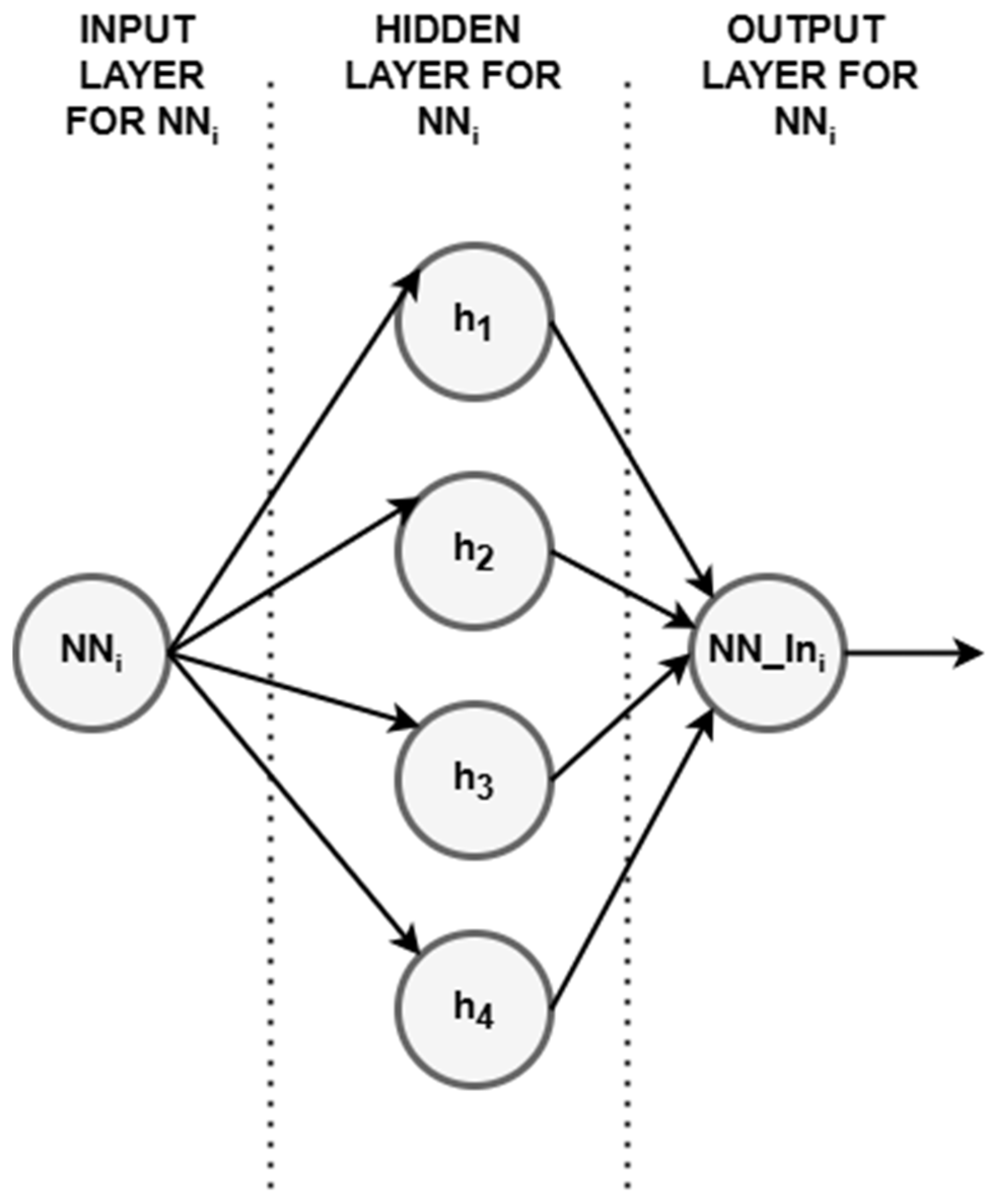
The FFNN used is described through the linear transformation, for the input layer (14)
where is the linear transformation for the input layer, is the weight matrix for the hidden layer, x is the data input vector, and is the bias vector for the hidden layer.
Each input data was processed through the feed-forward neural network (FFNN) to generate a learned representation or prediction, and an example is shown in Figure 5.

Figure 5.
Example of the FFNN with 4 neurons on the hidden layer used for simulation.
For the activation, the hyperbolic tangent sigmoid transfer function (15) was used.
where is the hyperbolic tangent sigmoid transfer function used as activation function applied to the input of a layer in the neural network.
The role of in (15) is to transform the input into a nonlinear output, , and the nonlinearity allows the network to learn complex patterns, rather than have just a linear function.
Moreover, the linear transformation (16) for the output layer is
where is the linear transformation for the output layer, is the weight matrix for the output layer, is the activation function, and is the bias vector for the output layer.
Finally, the output activation is as in (17)
where y represents the output of the FFNN.
After processing each input data vector and training with a FFNN containing four neurons in the hidden layer, the resulting output was used further in the mathematical modeling process [38].
Compared to more conventional models like ARIMA (AutoRegressive Integrated Moving Average), FFNNs are better at simulating intricate, nonlinear interactions in COVID-19 dynamics. Unlike ARIMA or exponential smoothing, which often need stationary time series, FFNNs may accept a variety of input sources, such as mobility, weather, and interventions.
The MISO model is made of five continuous transfer functions corresponding to each input.
With the control strategy proposed, the command signal obtained through the PI controller implementation is adjusting the process in such a way that it can control one input, but it can also control the prediction further.
A Multiple-Input Single-Output (MISO) system with five inputs and one output can be represented as in (18)
where represents the transfer functions for each input .
A Proportional-Integral (PI) controller is commonly used for MISO systems to regulate the output based on multiple inputs. The control law for a PI controller [39] is presented in (19)
where
- is the error signal for each input,
- is the proportional gain for input,
- is the integral gain for input,
- is the control action applied to the system.
For a Laplace domain representation, the PI controller [40] is given as in (20):
Thus, for a MISO system with a PI controller, the control signal from (21) is
where in (22) the error is described as follows:
The main purpose of this research was to demonstrate that, through specific controlled measures, the dynamics of the pandemic can be influenced, and even actively managed, with the goal of reducing its intensity.
Consequently, we initially considered three controllers—P, PI, and PID—as a case study. Both the P and PID controllers are represented in Figure 6.
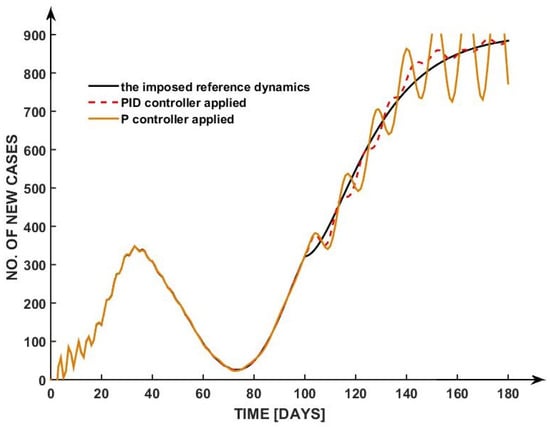
Figure 6.
Simulation results for PID and P controllers vs. the imposed reference dynamics.
For example, the PID controller is not justified because the generated command signal will have values higher than the imposed physical limits.
The oscillations in the P controller reflect its inability to handle dynamic changes and accumulated errors. A PI controller is often preferred over a PID controller in applications like epidemic control due to its simplicity, robustness, and reduced sensitivity to noise.
While the derivative component in a PID controller can improve response time by predicting future trends, it also tends to amplify high-frequency noise—common in real-world data such as daily reported COVID-19 cases—leading to unstable or overly aggressive control actions.
The PI controller, by focusing on correcting present and accumulated past errors, provides a smoother and more stable response, which is particularly important when implementing public health measures that must be gradual and predictable.
Thus, even if in the simulation we obtain better performances, the respective controller cannot be applied in the real world. However, as a future research direction, we suggest other control methods that will lead to improved regulation performance, that is, to a faster stabilization and no overregulation of the pandemic dynamics.
3. Results
3.1. Obtained Results and Simulations
To assess the performance of the proposed control strategy for mitigating the spread of COVID-19, the analysis of the predicted number of new cases over a period of 180 days under different control scenarios is presented. Figure 6 illustrates the evolution of the daily number of new cases with and without the proposed control actions.
As shown in Figure 6, the solid black line represents the imposed reference dynamics, which reflect the target trend that public health authorities aim to achieve in terms of controlling the number of new infections. The colored dashed and dotted lines represent the predicted dynamics under the application of three different instances of the proposed control strategy.
Figure 7 depicts a control strategy that was implemented in order to manage the COVID-19 pandemic over a period of one hundred and eighty days.
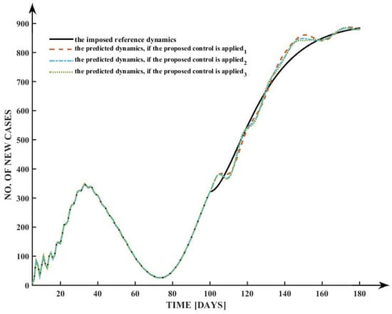
Figure 7.
Simulation results for three different types of control parameters.
The findings indicate that all three control mechanisms effectively steer the epidemic trajectory towards the reference dynamics, although with minor differences in convergence and overshooting characteristics. A peak of over 300 instances is recorded during the first 30 days, thereafter decreasing to less than 50 cases by day 70. Subsequently, a rebound emerges, culminating in around 900 new cases each day by day 150, which is effectively represented by all projected dynamics under the suggested restrictions.
The control solution approached is valid, as demonstrated in the manuscript, for the particular case of controlling the dynamics of the COVID-19 pandemic. It is obvious that for another type of pandemic or for different evolutions of the pandemic over time, the controller must be redesigned as an adaptive controller.
The proximity of all controlled trajectories to the reference trajectory confirms the robustness and efficacy of the suggested control mechanism. The controls have a notable capacity to adjust to intricate epidemic dynamics marked by many waves. Minor discrepancies of 5–10% are seen during the sharp rise in cases between days 100 and 140, with control (2) demonstrating marginally superior conformity to the reference trajectory in comparison to (1) and (3).
The findings underscore the capability of the proposed control mechanism to successfully manage pandemic waves and match epidemic outcomes with specified public health goals.
As part of their efforts to manage the COVID-19 pandemic, the authorities deployed a variety of control measures over the course of 180 days, which is approximately six months. Inferences can be made regarding the following timeline of interventions and the potential impact they could have based on the tendencies that are detected in the graph.
For tuning the PI controller for this MISO system, by applying the above presented equations, the values presented in Table 5 were determined for the proportional and integral constants of the controller:

Table 5.
Tuning parameters for PI controllers.
It indicates that the efforts were successful in controlling the outbreak by the time the 180-day period came to a conclusion, which consequently led to a plateau in the number of cases or hospitalizations. The fact that the two curves have converged indicates that the control measures have been more effective over time, which has reduced the number of outbreaks that have occurred.
3.2. Implementation Potential, Limitations, and Integration with Health System Dashboards
The proposed neural network-based predictive control system offers substantial potential for implementation in real-time public health decision-making. Its core strength lies in combining data-driven modeling through neural networks with control theory to predict and manage the spread of COVID-19 dynamically. The system uses a MISO neural network model to forecast future case numbers based on key variables such as testing rates, indoor and outdoor environmental conditions, and public health interventions.
The integration of a PI controller into a neural network-based control system for COVID-19 transmission provides a powerful yet practical tool for supporting real-time institutional decision-making. This approach leverages the forecasting capability of a trained neural network—capable of modeling complex, nonlinear dynamics of epidemic spread—combined with a PI control strategy that continuously adjusts intervention signals to minimize deviation from a desired reference trajectory (a target number of new daily cases). The PI controller, which corrects both the current and accumulated error between predicted and desired outcomes, enables stable and smooth responses, making it suitable for managing public health measures where abrupt or erratic changes are impractical.
The implementation potential of this system is high, particularly in regions with robust data reporting infrastructure. Key input variables may include the number of daily tests conducted, indoor and outdoor temperatures, outdoor humidity, and indicators of governmental policy interventions (such as lockdowns or mask mandates).
These inputs are processed through a trained neural network that estimates the future trajectory of infections. The PI controller then generates a control signal that minimizes the predicted deviation from the target scenario. This closed-loop structure enables institutions to respond adaptively and proportionately to changes in epidemic conditions.
However, the system’s effectiveness depends heavily on the quality and resolution of the input data. Inconsistent or delayed reporting of testing numbers or environmental factors can impair the neural network’s prediction accuracy, which in turn weakens the reliability of the control output.
Additionally, while the PI controller provides smoother control than a full PID controller (by avoiding sensitivity to noise in the derivative term), it may still struggle with delayed system responses or rapidly evolving epidemic phases if not properly tuned. Model retraining and periodic recalibration of controller parameters are necessary to maintain accuracy over time.
In the proposed control system, the command signal generated by the PI controller—ranging from 0 to 100—can be directly interpreted as a quantified level of public health intervention. This signal provides a continuous measure of the intensity of response required to keep COVID-19 transmission aligned with the desired trajectory.
A value near 0 indicates minimal or no intervention is needed, while a value approaching 100 suggests the need for maximum response, such as strict lockdowns or widespread testing and tracing. This numerical output can be mapped to specific, predefined policy actions (e.g., school closures, travel restrictions, mask mandates), allowing authorities to translate abstract control outputs into concrete, actionable measures. By incorporating this value into decision-making dashboards, institutions can track and adjust real-time response levels based on both epidemiological forecasts and operational capacity, thus enabling data-informed, proportionate, and timely interventions.
For effective integration with health system dashboards, the system should be designed to interface with platforms that public health institutions already use for data reporting and visualization. Integration would allow decision-makers to monitor current epidemic trends, view predictive outputs, and receive control recommendations within a unified interface.
Outputs could include real-time forecasts of case numbers, recommended levels of restrictions, and estimated outcomes of various intervention strategies. Visualization tools, such as trend graphs, control signal plots, and risk alerts, can make the system’s recommendations more understandable and actionable.
4. Conclusions
The current research provides a useful insight into the mathematical modeling for the number of active of COVID-19 cases prediction. A MISO model describes the prediction by analyzing actual data collected over a 60-day period. The prediction of the new COVID-19 cases expands starting with day 61 and continuing for 14 days. The accuracy of the output could be relevant for governmental institutions, supporting impactful decision-making in a future pandemic developments, particularly regarding the possible relaxation of regulations.
The 97.23% accuracy level obtained through the mathematical model developed in this study is an important indicator of its real-context applicability.
Moreover, by applying the control technique described in this research to new datasets gathered through future pandemics would allow a realistic simulation for new similar contexts before reaching critical points in its development. This approach could enhance the effectiveness of the decision-making process throughout real progress.
The data that could be provided for the mathematical method would consist in .csv files presenting sampled data in relation to time for number of tests conducted, indoor temperature, outdoor temperature, outdoor humidity, and quantified indicators of measures implemented by authorities to mitigate the spread of COVID-19.
Based on the previously described data input file, the predicted output for each date would consist of the number of new cases, new deaths, cumulative cases, and total fatalities displayed as a graph and saved as a .csv file as well.
On the other hand, the simulations could help inform the timely acquisition of specific medical equipment before the number of cases and overwhelms healthcare providers.
This method could be applied at both macro and micro levels within Romania. By inputting county-specific data, the model would generate distinct outputs tailored to address local challenges more effectively.
Author Contributions
Conceptualization, C.-M.S., I.A.Ș., V.M., I.C., M.A., M.-L.U., E.S., M.N., A.T. and I.N.; methodology: C.-M.S., I.A.Ș., V.M., I.C., M.A., M.-L.U., R.M., E.S., M.N., A.T. and I.N.; software: C.-M.S., I.A.Ș., V.M., I.C., M.A., M.-L.U. and R.M.; validation: C.-M.S., I.A.Ș., V.M., I.C., M.A., M.-L.U. and R.M.; formal analysis: C.-M.S., I.A.Ș., V.M. and I.C.; investigation: C.-M.S., I.A.Ș., V.B., V.M., I.C., M.A., M.-L.U., R.M., E.S., M.N., A.T. and I.N.; resource: C.-M.S., I.A.Ș., V.B., V.M., I.C., M.A., M.-L.U., R.M., E.S. and M.N.; data curation: C.-M.S., I.A.Ș., V.B., V.M., I.C., M.A., M.-L.U., R.M. and E.S.; writing—original draft preparation, C.-M.S., I.A.Ș., V.B., V.M., I.C., M.A., M.-L.U., R.M., E.S., M.N., A.T. and I.N.; writing—review and editing, C.-M.S., I.A.Ș., V.B., V.M., I.C. and M.A.; visualization: C.-M.S., I.A.Ș., V.B., V.M., I.C., M.A., M.-L.U., R.M., E.S., M.N., A.T. and I.N.; supervision: C.-M.S., V.B., V.M. and M.A.; project administration, C.-M.S., V.B. and M.A.; funding acquisition, C.-M.S., V.B., V.M. and M.A. All authors have read and agreed to the published version of the manuscript.
Funding
The current work was co-financed by Ministry of Education and Research of Romania funding through grant number PN-III-P2-2.1-SOL-2020-0157 (10Sol/2020), “The Dynamics of SARS-CoV-2 Virus Spread on Romanian Territory” and by the Technical University of Cluj-Napoca, Romania.
Data Availability Statement
The data presented in this study are available on request from the corresponding author due to privacy reasons.
Conflicts of Interest
The authors declare no conflicts of interest.
Abbreviations
The following abbreviations are used in this manuscript:
| MISO | Multiple-Input Single-Output |
| MIMO | Multiple-Input Multiple-Output |
| SISO | Single-Input Single-Output |
| WHO | World Health Organization |
| FFNN | Feed-forward neural network |
| PID | Proportional Integral Derivative |
| PHEIC | Public Health Emergency of International Concern |
| PI | Proportional Integral |
| LTI | Linear Time-Invariant |
References
- Andersen, K.G.; Rambaut, A.; Lipkin, W.I.; Holmes, E.C.; Garry, R.F. The proximal origin of SARS-CoV-2. Nat. Med. 2020, 26, 450–452. [Google Scholar] [CrossRef] [PubMed]
- WHO. Middle East Respiratory Syndrome Coronavirus (MERS-CoV). Available online: https://www.who.int/health-topics/middle-east-respiratory-syndrome-coronavirus-mers#tab=tab_2 (accessed on 15 October 2024).
- Drosten, C.; Günther, S.; Preiser, W.; van der Werf, S.; Brodt, H.R.; Becker, S.; Rabenau, H.; Panning, M.; Kolesnikova, L.; Fouchier, R.A.M.; et al. Identification of a novel coronavirus in patients with severe acute respiratory syndrome. N. Engl. J. Med. 2003, 348, 1967–1976. [Google Scholar] [CrossRef]
- Hoffmann, M.; Kleine-Weber, H.; Krüger, N.; Mueller, M.A.; Drosten, C.; Pöhlmann, S. The novel coronavirus 2019 (2019-nCoV) uses the SARS-coronavirus receptor ACE2 and the cellular protease TMPRSS2 for entry into target cells. Cell 2020, 181, 271–280.e8. [Google Scholar] [CrossRef]
- Li, Q.; Guan, X.; Wu, P.; Wang, X.; Zhou, L.; Tong, Y.; Ren, R.; Leung, K.S.M.; Lau, E.H.Y.; Wong, J.Y.; et al. Early transmission dynamics in Wuhan, China, of novel coronavirus–infected pneumonia. N. Engl. J. Med. 2020, 382, 1199–1207. [Google Scholar] [CrossRef]
- De Wit, E.; van Doremalen, N.; Falzarano, D.; Munster, V.J. SARS and MERS: Recent insights into emerging coronaviruses. Nat. Rev. Microbiol. 2016, 14, 523–534. [Google Scholar] [CrossRef]
- Wang, D.; Hu, B.; Hu, C.; Zhu, F.; Liu, X.; Zhang, J.; Wang, B.; Xiang, H.; Cheng, Z.; Xiong, Y.; et al. Clinical characteristics of 138 hospitalized patients with 2019 novel coronavirus–infected pneumonia in Wuhan, China. JAMA 2020, 323, 1061–1069. [Google Scholar] [CrossRef]
- Zhou, P.; Yang, X.L.; Wang, X.G.; Hu, B.; Zhang, L.; Zhang, W.; Si, H.R.; Zhu, Y.; Li, B.; Huang, C.L.; et al. A pneumonia outbreak associated with a new coronavirus of probable bat origin. Nature 2020, 579, 270–273. [Google Scholar] [CrossRef]
- World Health Organization. Coronavirus Disease (COVID-19) Pandemic. Available online: https://www.who.int/europe/emergencies/situations/covid-19 (accessed on 15 October 2024).
- European Commission. Coronavirus Response. Available online: https://commission.europa.eu/strategy-and-policy/coronavirus-response_en (accessed on 15 October 2024).
- European Central Bank. The Heterogeneous Economic Impact of the Pandemic Across Euro Area Countries. Available online: https://www.ecb.europa.eu/press/economic-bulletin/focus/2021/html/ecb.ebbox202105_03~267ada0d38.en.html (accessed on 15 October 2024).
- Rees, G.H.; Batenburg, R.; Scotter, C. Responding to COVID-19: An exploration of EU country responses and directions for further research. BMC Health Serv. Res. 2024, 24, 1198. [Google Scholar] [CrossRef]
- International Monetary Fund. Policy Responses to COVID-19. Available online: https://www.imf.org/en/Topics/imf-and-covid19/Policy-Responses-to-COVID-19 (accessed on 15 October 2024).
- United Nations Statistics Division. UNSD—Demographic and Social Statistics. Available online: https://unstats.un.org/unsd/demographic-social/census/COVID-19/ (accessed on 15 October 2024).
- Streinu-Cercel, A.; Apostolescu, C.; Săndulescu, O.; Oţelea, D.; Streinu-Cercel, A.; Vlaicu, O.; Paraschiv, S.; Benea, O.E.; Bacruban, R.; Niţescu, M.; et al. SARS-CoV-2 in Romania-analysis of the first confirmed case and evolution of the pandemic in Romania in the first three months. Germs 2020, 10, 132–134. [Google Scholar] [CrossRef] [PubMed] [PubMed Central]
- Horga, N.G.; Cirnatu, D.; Kundnani, N.R.; Ciurariu, E.; Parvu, S.; Ignea, A.L.; Borza, C.; Sharma, A.; Morariu, S. Evaluation of Non-Pharmacological Measures Implemented in the Management of the COVID-19 Pandemic in Romania. Healthcare 2022, 10, 1756. [Google Scholar] [CrossRef]
- State of Health in the EU—Romania: Country Health Profile 2021. Available online: https://health.ec.europa.eu/system/files/2021-12/2021_chp_romania_english.pdf (accessed on 15 October 2024).
- Briciu, V.; Leucuta, D.C.; Muntean, M.; Radulescu, A.; Cismaru, C.; Topan, A.; Herbel, L.; Horvat, M.; Calin, M.; Dobrota, R.; et al. Evolving Clinical Manifestations and Outcomes in COVID-19 Patients: A Comparative Analysis of SARS-CoV-2 Variant Waves in a Romanian Hospital Setting. Pathogens 2023, 12, 1453. [Google Scholar] [CrossRef]
- Hâncean, M.G.; Perc, M.; Lerner, J. Early spread of COVID-19 in Romania: Imported cases from Italy and human-to-human transmission networks. R. Soc. Open Sci. 2020, 7, 200780. [Google Scholar] [CrossRef]
- Montesó-Curto, P.; Sánchez-Montesó, L.; Maramao, F.S.; Toussaint, L. Coping with the COVID-19 Pandemic in Italy and Spain: Lessons in Response Urgency. J. Glob. Health 2020, 10, 020326. [Google Scholar] [CrossRef] [PubMed] [PubMed Central]
- European Observatory OECD on Health Systems and Policies Romania. Country Health Profile 2019: European Observatory on Health Systems and Policies; OECD Publishing: Paris, France; Brussels, Belgium, 2019. [Google Scholar]
- Gunasekaran, N.; Vadivel, R.; Zhai, G.; Vinoth, S. Finite-time stability analysis and control of stochastic SIR epidemic model: A study of COVID-19. Biomed. Signal Process. Control. 2023, 86 Pt A, 105123. [Google Scholar] [CrossRef] [PubMed]
- Bandekar, S.R.; Ghosh, M.; Rajivganthi, C. Impact of vaccination on the dynamics of COVID-19: A mathematical study using fractional derivatives. Int. J. Biomath. 2023, 17, 2350018. [Google Scholar] [CrossRef]
- Fadaei, Y.; Rihan, F.A.; Rajivganthi, C. Immunokinetic Model for COVID-19 Patients. Complexity 2022, 2022, 8321848. [Google Scholar] [CrossRef]
- Wei, Y.; Dong, Z.; Fan, W.; Xu, K.; Tang, S.; Wang, Y.; Wu, F. A narrative review on the role of temperature and humidity in COVID-19: Transmission, persistence, and epidemiological evidence. Eco-Environ. Health 2022, 1, 73–85. [Google Scholar] [CrossRef] [PubMed] [PubMed Central]
- Haq, F.U.; Abduljaleel, Y.; Ahmad, I. Effect of temperature on fast transmission of COVID-19 in low per capita GDP Asian countries. Sci. Rep. 2023, 13, 21165. [Google Scholar] [CrossRef]
- Shi, P.; Dong, Y.; Yan, H.; Zhao, C.; Li, X.; Liu, W.; He, M.; Tang, S.; Xi, S. Impact of temperature on the dynamics of the COVID-19 outbreak in China. Sci. Total Environ. 2020, 728, 138890. [Google Scholar] [CrossRef] [PubMed] [PubMed Central]
- Ahlawat, A.; Wiedensohler, A.; Mishra, S. An Overview on the Role of Relative Humidity in Airborne Transmission of SARS-CoV-2 in Indoor Environments. Aerosol Air Qual. Res. 2020, 20, 1856–1861. [Google Scholar] [CrossRef]
- Lednicky, J.A.; Lauzardo, M.; Fan, Z.H.; Jutla, A.; Tilly, T.B.; Gangwar, M.; Usmani, M.; Shankar, S.N.; Mohamed, K.; Eiguren-Fernandez, A.; et al. Viable SARS-CoV-2 in the air of a hospital room with COVID-19 patients. Int. J. Infect. Dis. 2020, 100, 476–482. [Google Scholar] [CrossRef] [PubMed] [PubMed Central]
- Boulos, L.; Curran, J.A.; Gallant, A.; Wong, H.; Johnson, C.; Delahunty-Pike, A.; Saxinger, L.; Chu, D.; Comeau, J.; Flynn, T.; et al. Effectiveness of face masks for reducing transmission of SARS-CoV-2: A rapid systematic review. Philos. Trans. A Math. Phys. Eng. Sci. 2023, 381, 20230133. [Google Scholar] [CrossRef] [PubMed] [PubMed Central]
- Addleman, S.; Leung, V.; Asadi, L.; Sharkawy, A.; McDonald, J. Mitigating airborne transmission of SARS-CoV-2. CMAJ 2021, 193, E1010–E1011. [Google Scholar] [CrossRef] [PubMed] [PubMed Central]
- Yamasaki, L.; Murayama, H.; Hashizume, M. The impact of temperature on the transmissibility and virulence of COVID-19 in Tokyo, Japan. Sci. Rep. 2021, 11, 24477. [Google Scholar] [CrossRef]
- Ayouni, I.; Maatoug, J.; Dhouib, W.; Zammit, N.; Fredj, S.B.; Ghammam, R. Effective public health measures to mitigate the spread of COVID-19: A systematic review. BMC Public Health 2021, 21, 1015. [Google Scholar] [CrossRef]
- Silva, T.C.; Anghinoni, L.; Chagas, C.P.d.; Zhao, L.; Tabak, B.M. Analysis of the Effectiveness of Public Health Measures on COVID-19 Transmission. Int. J. Environ. Res. Public Health 2023, 20, 6758. [Google Scholar] [CrossRef]
- Feurer, D.; Tim, R.; Maxi Stella, K.; Enrique, A.; Ben, A.; Malcolm, M.; Rachel, L.; Dominic, R.; Masahiro, H.; Lina, M.; et al. Meteorological factors, population immunity, and COVID-19 incidence: A global multi-city analysis. Environ. Epidemiol. 2024, 8, e338. [Google Scholar] [CrossRef] [PubMed] [PubMed Central]
- Kuwahara, B.; Bauch, C.T. Predicting Covid-19 pandemic waves with biologically and behaviorally informed universal differential equations. Heliyon 2024, 10, e25363. [Google Scholar] [CrossRef]
- Ali, S.; Riaz, S.; Liu, X.; Wang, G. A Levenberg–Marquardt Based Neural Network for Short-Term Load Forecasting. Comput. Mater. Contin. 2023, 75, 1783–1800. [Google Scholar] [CrossRef]
- Ruttanaprommarin, N.; Sabir, Z.; Núñez, R.A.S.; Az-Zobi, E.; Weera, W.; Botmart, T.; Zamart, C. A Stochastic Framework for Solving the Prey-Predator Delay Differential Model of Holling Type-III. Comput. Mater. Contin. 2023, 74, 5915–5930. [Google Scholar] [CrossRef]
- Stăncioi, C.-M.; Ștefan, I.A.; Briciu, V.; Mureșan, V.; Clitan, I.; Abrudean, M.; Ungureșan, M.-L.; Miron, R.; Stativă, E.; Nanu, M.; et al. Solution for the Mathematical Modeling and Future Prediction of the COVID-19 Pandemic Dynamics. Appl. Sci. 2023, 13, 7971. [Google Scholar] [CrossRef]
- Dogruer, T.; Tan, N. Design of PI Controller using Optimization Method in Fractional Order Control Systems. IFAC-PapersOnLine 2018, 51, 841–846. [Google Scholar] [CrossRef]
Disclaimer/Publisher’s Note: The statements, opinions and data contained in all publications are solely those of the individual author(s) and contributor(s) and not of MDPI and/or the editor(s). MDPI and/or the editor(s) disclaim responsibility for any injury to people or property resulting from any ideas, methods, instructions or products referred to in the content. |
© 2025 by the authors. Licensee MDPI, Basel, Switzerland. This article is an open access article distributed under the terms and conditions of the Creative Commons Attribution (CC BY) license (https://creativecommons.org/licenses/by/4.0/).

