Finite Integration Method with Chebyshev Expansion for Shallow Water Equations over Variable Topography

Abstract

The shallow water equations (SWEs) model fluid flow in rivers, coasts, and tsunamis. Their nonlinearity challenges analytical solutions. We present a numerical algorithm combining the finite integration method with Chebyshev polynomial expansion (FIM-CPE) to solve one- and two-dimensional SWEs. The method transforms partial differential equations into integral equations, approximates spatial terms via Chebyshev polynomials, and uses forward differences for time discretization. Validated on stationary lakes, dam breaks, and Gaussian pulses, the scheme achieved errors below ${10}^{-12}$ for water height and velocity, while conserving mass with volume deviations under ${10}^{-5}$. Comparisons showed superior shock-capturing versus finite difference methods. For two-dimensional cases, it accurately resolved wave interactions over complex topographies. Though limited to wet beds and small-scale two-dimensional problems, the method provides a robust simulation tool.

1. Introduction

The shallow water equations (SWEs), first introduced by Saint-Venant [1] in 1871 to model open-channel flow, are also referred to as Saint-Venant’s equations. These equations form a mathematical model for understanding water movement in shallow regions such as rivers and beaches. They find applications in simulating various phenomena, including dam breaks, tsunamis, and floods, see [2,3,4,5] for more details. The behavior of these flows is also influenced by the bottom topography, and significant research has been dedicated to wave interactions over various topographies [6]. Study of the SWEs facilitates the analysis of how topography affects water flow.

The shallow water model is predicated on the assumption that the horizontal length scale of the flow is significantly larger than the water’s depth. This assumption permits a simplification of the governing equations by averaging the mass and momentum conservation equations over the depth, thereby eliminating the vertical dimension. The SWEs manifest as a system of partial differential equations (PDEs) that characterize shallow water behavior through its height and velocity. They are derived from the principles of mass and momentum conservation. The model comprises two main components. The first is the continuity equation, which arises from the conservation of mass and describes the temporal variation in water height, accounting for water flux into and out of a given area. The second component is the momentum equation, derived from momentum conservation principles, which governs the horizontal movement of water. This equation considers the forces acting on the water, notably gravity and pressure gradients, that influence its velocity. Assuming frictionless flow over a wet bottom topography, the one- and two-dimensional SWEs can be expressed without a friction term, similarly to the formulation in [7]. The one-dimensional SWEs are then given by

$$\left\{\begin{array}{cc}\hfill & {\displaystyle \frac{\partial h}{\partial t}}+{\displaystyle \frac{\partial }{\partial x}}\left(hu\right)=0,\hfill \\ \hfill & {\displaystyle \frac{\partial }{\partial t}}\left(hu\right)+{\displaystyle \frac{\partial }{\partial x}}\left(h{u}^2+{\displaystyle \frac{g{h}^2}{2}}\right)=-gh{\displaystyle \frac{\partial z}{\partial x}},\hfill \end{array}\right.$$

(1)

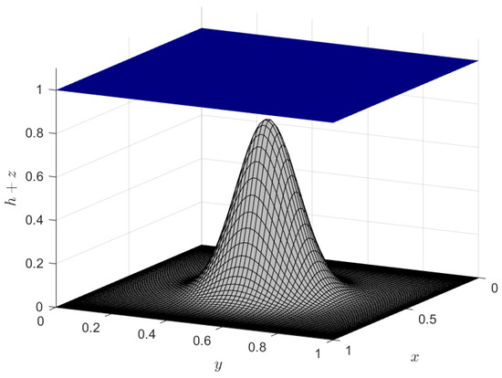
where x is the spatial variable, t is the temporal variable, h represents the water height, u is the horizontal velocity, g is the gravitational constant, and z denotes the bottom topography, as visualized in Figure 1a. The two-dimensional SWEs extend the one-dimensional model by incorporating the spatial variable y and its associated velocity component:

$$\left\{\begin{array}{cc}\hfill & {\displaystyle \frac{\partial h}{\partial t}}+{\displaystyle \frac{\partial }{\partial x}}\left(hu\right)+{\displaystyle \frac{\partial }{\partial y}}\left(hv\right)=0,\hfill \\ \hfill & {\displaystyle \frac{\partial }{\partial t}}\left(hu\right)+{\displaystyle \frac{\partial }{\partial x}}\left(h{u}^2+{\displaystyle \frac{g{h}^2}{2}}\right)+{\displaystyle \frac{\partial }{\partial y}}\left(huv\right)=-gh{\displaystyle \frac{\partial z}{\partial x}},\hfill \\ \hfill & {\displaystyle \frac{\partial }{\partial t}}\left(hv\right)+{\displaystyle \frac{\partial }{\partial x}}\left(huv\right)+{\displaystyle \frac{\partial }{\partial y}}\left(h{v}^2+{\displaystyle \frac{g{h}^2}{2}}\right)=-gh{\displaystyle \frac{\partial z}{\partial y}},\hfill \end{array}\right.$$

(2)

where x and y are the spatial variables, and u and v are the horizontal velocity components in their respective directions, as depicted in Figure 1b.

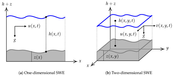
Figure 1. Physical variables for one- and two-dimensional shallow water models.

The SWEs are a nonlinear hyperbolic system of conservation equations that include a source term for topography, making their analytical solution challenging. Consequently, numerical methods are essential for simulating water flow. A diverse set of numerical schemes has been developed to solve the SWEs. These include Finite Difference Methods (FDMs), such as those by Hudson [8] and Crowhurst and Li [9], which are often straightforward to implement but can face challenges with complex topographies and shock capturing. In contrast, Finite Volume Methods (FVMs), such as the adaptive FVM by Peng [10] and Godunov-type methods by LeVeque [11], are well-regarded for their conservation properties and robust shock-capturing capabilities. For scenarios requiring a higher precision with smooth solutions, high-order approaches like the Spectral Difference Method (SDM) by San and Kara [12] and the Summation-By-Parts Operators with Simultaneous Approximation Terms (SBP-SAT) by Lundgren [13] offer excellent accuracy, though often at the cost of increased complexity. While methods based on a fundamental solution, or Green’s function, can be powerful, a simple Green’s function is not available for the full nonlinear SWEs, necessitating the development of direct numerical methods.

A common feature of many of these methods is their reliance on differential approximation, which can be sensitive to round-off errors, especially with small spatial step sizes. To address this limitation, this paper presents a Finite Integration Method with Chebyshev Polynomial Expansion (FIM-CPE) [14], a technique that transforms the governing PDEs into integral equations, before discretization to mitigate round-off errors. Because our method operates on an integral form, it is relevant to situate it with respect to other established techniques for solving integral equations. Unlike weighted residual methods such as the Galerkin method, which require complex inner product integrations, our FIM-CPE is a collocation-based approach. It ensures that the integral equation is satisfied exactly at a discrete set of points (the zeros of Chebyshev), often leading to a more straightforward formulation. This approach, combined with the spectral accuracy of Chebyshev polynomial expansions, enables a high-order accurate algorithm, see [15,16,17] for more details. The primary objective of this work is to develop a robust numerical algorithm using FIM-CPE for the accurate simulation of one- and two-dimensional SWEs and to validate its effectiveness in resolving both smooth and discontinuous solutions across various topographies.

2. Developed FIM-CPE

This section details the construction of one- and two-dimensional Chebyshev integration matrices, which form the cornerstone of the FIM-CPE. We begin by defining Chebyshev polynomials and outlining their key properties, as established in [15].

Chebyshev polynomials are specifically chosen for this work due to their optimal properties in function approximation. They possess the minimax property, which minimizes the maximum approximation error over the interval. Furthermore, the use of Chebyshev nodes for collocation, which are the roots of the polynomials, clusters points near the boundaries. This non-uniform distribution is highly effective at mitigating Runge’s phenomenon, preventing the large oscillations that can occur at the edges of an interval when using equally spaced points with high-degree polynomials.

Definition 1

([15]). The Chebyshev polynomial of degree $n\ge 0$ is defined by

$$R_n\left(x\right)=\cos \left(narccos\left({\displaystyle \frac{2x-a-b}{b-a}}\right)\right)forx\in [a,b].$$

(3)

Lemma 1

([15]). The following are properties of the Chebyshev polynomials:

(i)

The zeros of the Chebyshev polynomial $R_n\left(x\right)$ for $x\in [a,b]$ are given by

$$x_k={\displaystyle \frac{1}{2}}\left((b-a)\cos \left({\displaystyle \frac{2k-1}{2n}}\pi \right)+a+b\right),k\in \{1,2,3,\dots ,n\}.$$

(4)

(ii)

The single-layer integrals of the Chebyshev polynomial $R_n\left(x\right)$ are given for $n\ge 2$ by

$$\begin{array}{cc}\hfill {\overline{R}}_0\left(x\right)={\int }_a^x{R}_0\left(\xi \right)d\xi & =x-a,\hfill \\ \hfill {\overline{R}}_1\left(x\right)={\int }_a^x{R}_1\left(\xi \right)d\xi & ={\displaystyle \frac{(x-a)(x-b)}{b-a}},\hfill \\ \hfill {\overline{R}}_n\left(x\right)={\int }_a^x{R}_n\left(\xi \right)d\xi & ={\displaystyle \frac{b-a}{4}}\left({\displaystyle \frac{R_{n+1}\left(x\right)}{n+1}}-{\displaystyle \frac{R_{n-1}\left(x\right)}{n-1}}-{\displaystyle \frac{2{(-1)}^n}{n^2-1}}\right).\hfill \end{array}$$

(iii)

The Chebyshev matrix $\mathbf{R}$ at each zero $x_k$ defined in (4) is given by

$$\mathbf{R}=\left[\begin{array}{cccc}{R}_0\left(x_1\right)& R_1\left(x_1\right)& \cdots & R_{n-1}\left(x_1\right)\\ R_0\left(x_2\right)& R_1\left(x_2\right)& \cdots & R_{n-1}\left(x_2\right)\\ ⋮& ⋮& \ddots & ⋮\\ R_0\left(x_n\right)& R_1\left(x_n\right)& \cdots & R_{n-1}\left(x_n\right)\end{array}\right].$$

Its multiplicative inverse is ${\mathbf{R}}^{-1}={\displaystyle \frac{1}{n}}\mathrm{diag}\{1,2,2,\dots ,2\}{\mathbf{R}}^{\top }$.

For the construction of a two-dimensional Chebyshev integration matrix, it is essential to introduce the Kronecker product [18] and its properties.

Definition 2

([18]). Let $\mathbf{A}=\left[a_{ij}\right]\in {\mathbb{R}}^{m\times n}$ and $\mathbf{B}=\left[b_{ij}\right]\in {\mathbb{R}}^{p\times q}.$ Then, the Kronecker product $\mathbf{A}\otimes \mathbf{B}\in {\mathbb{R}}^{mp\times nq}$ is defined by the block matrix as follows:

$$\mathbf{A}\otimes \mathbf{B}=\left[\begin{array}{ccc}{a}_{11}\mathbf{B}& \dots & a_{1n}\mathbf{B}\\ ⋮& \ddots & ⋮\\ a_{m1}\mathbf{B}& \dots & a_{mn}\mathbf{B}\end{array}\right].$$

Theorem 1

([18]). The Kronecker product possesses the following characteristics:

(i)

Let $\mathbf{A}\in {\mathbb{R}}^{m\times n}$, $\mathbf{B}\in {\mathbb{R}}^{p\times q}$ and ${\mathbf{I}}_k$ denote an $k\times k$ identity matrix. Then,

$$\mathbf{A}\otimes \mathbf{B}=(\mathbf{A}\otimes {\mathbf{I}}_p)({\mathbf{I}}_m\otimes \mathbf{B})=({\mathbf{I}}_m\otimes \mathbf{B})(\mathbf{A}\otimes {\mathbf{I}}_q).$$

(ii)

Let $\mathbf{A}\in {\mathbb{R}}^{m\times n}$, $\mathbf{B}\in {\mathbb{R}}^{p\times q}$, $\mathbf{C}\in {\mathbb{R}}^{n\times r}$, and $\mathbf{D}\in {\mathbb{R}}^{q\times s}$. Then,

$$(\mathbf{A}\otimes \mathbf{B})(\mathbf{C}\otimes \mathbf{D})=\left(\mathbf{AC}\right)\otimes \left(\mathbf{BD}\right).$$

(iii)

Let $\mathbf{A}\in {\mathbb{R}}^{m\times m}$ and $\mathbf{B}\in {\mathbb{R}}^{n\times n}$. Let ${\mathbf{e}}_i$ be an $m\times 1$ standard unit vector with a 1 in the i-th position and 0s elsewhere, i.e., ${\mathbf{e}}_i={[0,\dots ,0,1,0,\dots ,0]}^{\top }$. If an $mn\times mn$ permutation matrix is defined as $\mathbf{P}=[{\mathbf{I}}_n\otimes {\mathbf{e}}_1, {\mathbf{I}}_n\otimes {\mathbf{e}}_2,\dots , {\mathbf{I}}_n\otimes {\mathbf{e}}_m]$, then $\mathbf{P}(\mathbf{A}\otimes \mathbf{B}){\mathbf{P}}^{\top }=\mathbf{B}\otimes \mathbf{A}$.

2.1. One-Dimensional Chebyshev Integration Matrix

Next, we construct the one-dimensional Chebyshev integration matrix, which is instrumental for handling integral terms. First, let $M\in \mathbb{N}$ and $a<b\in \mathbb{R}$. Consider a function f that can be approximated by the Chebyshev polynomial expansion

$$f\left(x\right)=\sum _{n=0}^{M-1}{c}_{f,n}{R}_n\left(x\right)\mathrm{for}x\in [a,b],$$

(5)

where $c_{f,n}$ are the unknown coefficients of the function f to be determined and $R_n\left(x\right)$ are the Chebyshev polynomials of degree n as defined in (3). Let $x_1<x_2<\dots <x_M\in [a,b]$ be nodal points discretized by the zeros of the Chebyshev polynomial $R_M\left(x\right)$, as defined in (4). Substituting each $x_k$ into (5), the expression can be written in matrix form as

$$\left[\begin{array}{c}f\left(x_1\right)\\ f\left(x_2\right)\\ ⋮\\ f\left(x_M\right)\end{array}\right]=\left[\begin{array}{cccc}{R}_0\left(x_1\right)& R_1\left(x_1\right)& \cdots & R_{M-1}\left(x_1\right)\\ R_0\left(x_2\right)& R_1\left(x_2\right)& \cdots & R_{M-1}\left(x_2\right)\\ ⋮& ⋮& \ddots & ⋮\\ R_0\left(x_M\right)& R_1\left(x_M\right)& \cdots & R_{M-1}\left(x_M\right)\end{array}\right]\left[\begin{array}{c}{c}_{f,0}\\ c_{f,1}\\ ⋮\\ c_{f,M-1}\end{array}\right].$$

This is compactly denoted by $\mathbf{f}={\mathbf{Rc}}_f$. Consequently, the coefficient vector ${\mathbf{c}}_f$ can be expressed as ${\mathbf{c}}_f={\mathbf{R}}^{-1}\mathbf{f}$, where ${\mathbf{R}}^{-1}$ is defined in Lemma 1(iii). Next, we consider the single-layer integral of f from a to $x_k$, denoted by $F\left(x_k\right)$:

$$F\left(x_k\right)={\int }_a^{x_k}f\left(\xi \right)d\xi =\sum _{n=0}^{M-1}{c}_{f,n}{\int }_a^{x_k}{R}_n\left(\xi \right)d\xi =\sum _{n=0}^{M-1}{c}_{f,n}{\overline{R}}_n\left(x_k\right),$$

(6)

for $k\in \{1,2,3,\dots ,M\}$, where each ${\overline{R}}_n\left(x_k\right)$ is defined in Lemma 1(ii). In matrix form, this becomes

$$\left[\begin{array}{c}F\left(x_1\right)\\ F\left(x_2\right)\\ ⋮\\ F\left(x_M\right)\end{array}\right]=\left[\begin{array}{cccc}{\overline{R}}_0\left(x_1\right)& {\overline{R}}_1\left(x_1\right)& \cdots & {\overline{R}}_{M-1}\left(x_1\right)\\ {\overline{R}}_0\left(x_2\right)& {\overline{R}}_1\left(x_2\right)& \cdots & {\overline{R}}_{M-1}\left(x_2\right)\\ ⋮& ⋮& \ddots & ⋮\\ {\overline{R}}_0\left(x_M\right)& {\overline{R}}_1\left(x_M\right)& \cdots & {\overline{R}}_{M-1}\left(x_M\right)\end{array}\right]\left[\begin{array}{c}{c}_{f,0}\\ c_{f,1}\\ ⋮\\ c_{f,M-1}\end{array}\right].$$

This is compactly denoted by $\mathbf{F}=\overline{\mathbf{R}}{\mathbf{c}}_f$. Substituting ${\mathbf{c}}_f={\mathbf{R}}^{-1}\mathbf{f}$, we obtain $\mathbf{F}=\overline{\mathbf{R}}{\mathbf{R}}^{-1}\mathbf{f}$. We then define $\mathbf{A}:=\overline{\mathbf{R}}{\mathbf{R}}^{-1}={\left[a_{ki}\right]}_{M\times M}$ as the `one-dimensional Chebyshev integration matrix’. Thus, $\mathbf{F}=\mathbf{Af}$ and (6) can be written in terms of discrete values as

$$F\left(x_k\right)={\int }_a^{x_k}f\left(\xi \right)d\xi =\sum _{i=1}^M{a}_{ki}f\left(x_i\right).$$

(7)

2.2. Two-Dimensional Chebyshev Integration Matrix

Let $M,N\in \mathbb{N}$ and $a,b,c,d\in \mathbb{R}$. The computational nodes $x_k$ and $y_k$ are defined over the domain $[a,b]\times [c,d]$, corresponding to the zeros of Chebyshev polynomials $R_M\left(x\right)$ and $R_N\left(y\right)$ along the horizontal and vertical directions, respectively. For convenience, we use a global numbering system for grid points along the x-direction (Figure 2a) and a local numbering system for the y-direction (Figure 2b).

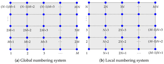
Figure 2. The indices of the grid points globally and locally.

Let us consider the single-layer integrals with respect to the variables x and y, denoted by $F_x(x,y)$ and $F_y(x,y)$, respectively. Using (7) with a fixed constant y, we can express $F_x(x_k,y)$ in the global numbering system as

$$F_x(x_k,y)={\int }_a^{x_k}f(\xi ,y)d\xi =\sum _{i=1}^M{a}_{ki}f(x_i,y).$$

(8)

For $k\in \{1,2,3,\dots ,M\}$, (8) can be expressed by ${\mathbf{F}}_x(·,y)={\mathbf{A}}_M\mathbf{f}(·,y),$ where ${\mathbf{A}}_M=\overline{\mathbf{R}}{\mathbf{R}}^{-1}$ is an $M\times M$ matrix. Thus, for each varying $y\in \{y_1,y_2,y_3,\dots ,y_N\}$, we form a block matrix:

$$\left[\begin{array}{c}{\mathbf{F}}_x(·,y_1)\\ {\mathbf{F}}_x(·,y_2)\\ ⋮\\ {\mathbf{F}}_x(·,y_N)\end{array}\right]=\underset{N\mathrm{blocks}}{\underbrace{\left[\begin{array}{cccc}{\mathbf{A}}_M& 0& \cdots & 0\\ 0& {\mathbf{A}}_M& \ddots & ⋮\\ ⋮& \ddots & \ddots & 0\\ 0& \cdots & 0& {\mathbf{A}}_M\end{array}\right]}}\left[\begin{array}{c}\mathbf{f}(·,y_1)\\ \mathbf{f}(·,y_2)\\ ⋮\\ \mathbf{f}(·,y_N)\end{array}\right].$$

This is denoted by ${\mathbf{F}}_x={\mathbf{A}}_x\mathbf{f},$ where ${\mathbf{A}}_x={\mathbf{I}}_N\otimes {\mathbf{A}}_M$ is the ‘two-dimensional Chebyshev integration matrix along the x-axis’. Similarly, using (7) with a fixed constant x, we have

$$F_y(x,y_h)={\int }_c^{y_h}f(x,\eta )d\eta =\sum _{j=1}^N{a}_{hj}f(x,y_j).$$

(9)

For $h\in \{1,2,3,\dots ,N\}$, (9) can be expressed by ${\mathbf{F}}_y(x,·)={\mathbf{A}}_N\mathbf{f}(x,·),$ where ${\mathbf{A}}_N=\overline{\mathbf{R}}{\mathbf{R}}^{-1}$ is an $N\times N$ matrix. Thus, for each varying $x\in \{x_1,x_2,x_3,\dots ,x_M\}$, we obtain a block matrix:

$$\left[\begin{array}{c}{\mathbf{F}}_y(x_1,·)\\ {\mathbf{F}}_y(x_2,·)\\ ⋮\\ {\mathbf{F}}_y(x_M,·)\end{array}\right]=\underset{M\mathrm{blocks}}{\underbrace{\left[\begin{array}{cccc}{\mathbf{A}}_N& 0& \cdots & 0\\ 0& {\mathbf{A}}_N& \ddots & ⋮\\ ⋮& \ddots & \ddots & 0\\ 0& \cdots & 0& {\mathbf{A}}_N\end{array}\right]}}\left[\begin{array}{c}\mathbf{f}(x_1,·)\\ \mathbf{f}(x_2,·)\\ ⋮\\ \mathbf{f}(x_M,·)\end{array}\right].$$

This is denoted by ${\tilde{\mathbf{F}}}_y={\tilde{\mathbf{A}}}_y\tilde{\mathbf{f}},$ where ${\tilde{\mathbf{A}}}_y={\mathbf{I}}_M\otimes {\mathbf{A}}_N$ and $\tilde{\mathbf{f}}$ is in the local numbering system. Note that the elements of $\mathbf{f}$ and $\tilde{\mathbf{f}}$ are the same values, but their positions differ in the numbering systems. Thus, we can transform ${\tilde{\mathbf{F}}}_y$ and $\tilde{\mathbf{f}}$ from local to global numbering systems using a permutation matrix $\mathbf{P}={\left[p_{ij}\right]}_{MN\times MN},$ where each $p_{ij}$ is defined by

$$p_{ij}=\left\{\begin{array}{cc}1\hfill & ;i=(h-1)M+k\mathrm{and}j=(k-1)N+h,\hfill \\ 0\hfill & ;\mathrm{otherwise},\hfill \end{array}\right.$$

(10)

for all $k\in \{1,2,3,\dots ,M\}$ and $h\in \{1,2,3,\dots ,N\}$. We obtain that ${\mathbf{F}}_y=\mathbf{P}{\tilde{\mathbf{F}}}_y$ and $\mathbf{f}=\mathbf{P}\tilde{\mathbf{f}}.$ Therefore, ${\mathbf{F}}_y={\mathbf{A}}_y\mathbf{u}$, where ${\mathbf{A}}_y=\mathbf{P}{\tilde{\mathbf{A}}}_y{\mathbf{P}}^{-1}=\mathbf{P}({\mathbf{I}}_M\otimes {\mathbf{A}}_N){\mathbf{P}}^{\top }$ is the `two-dimensional Chebyshev integration matrix along the y-axis’ in the global numbering system.

Next, we consider the double-layer integral with respect to both variables x and y, denoted by $F_{xy}(x_k,y_h)$. By using (8) and (9), we have

$$F_{xy}(x_k,y_h)={\int }_c^{y_h}{\int }_a^{x_k}f(\xi ,\eta )d\xi d\eta =\sum _{j=1}^N\sum _{i=1}^M{a}_{hj}{a}_{ki}f(x_i,y_j).$$

(11)

For $k\in \{1,2,3,\dots ,M\}$ and $h\in \{1,2,3,\dots ,N\}$, this can be analyzed as two types:

• Type I: If $y_h$ is fixed but $x_k$ is varied, (11) becomes ${\mathbf{F}}_{xy}(·,y_h)={\sum }_{j=1}^N{a}_{hj}{\mathbf{A}}_M\mathbf{f}(·,y_j)$, where $a_{hj}$ is an element of the Chebyshev integration matrix ${\mathbf{A}}_N$ at position $(h,j)$. By varying all $y_h\in \{y_1,y_2,y_3,\dots ,y_N\}$, we obtain the block matrix:

  $$\left[\begin{array}{c}{\mathbf{F}}_{xy}(·,y_1)\\ {\mathbf{F}}_{xy}(·,y_2)\\ ⋮\\ {\mathbf{F}}_{xy}(·,y_N)\end{array}\right]=\left[\begin{array}{cccc}{a}_{11}{\mathbf{I}}_M& a_{12}{\mathbf{I}}_M& \cdots & a_{1N}{\mathbf{I}}_M\\ a_{21}{\mathbf{I}}_M& a_{22}{\mathbf{I}}_M& \cdots & a_{2N}{\mathbf{I}}_M\\ ⋮& ⋮& \ddots & ⋮\\ a_{N1}{\mathbf{I}}_M& a_{N2}{\mathbf{I}}_M& \cdots & a_{NN}{\mathbf{I}}_M\end{array}\right]\underset{N\mathrm{blocks}}{\underbrace{\left[\begin{array}{cccc}{\mathbf{A}}_M& 0& \cdots & 0\\ 0& {\mathbf{A}}_M& \ddots & ⋮\\ ⋮& \ddots & \ddots & 0\\ 0& \cdots & 0& {\mathbf{A}}_M\end{array}\right]}}\left[\begin{array}{c}\mathbf{f}(·,y_1)\\ \mathbf{f}(·,y_2)\\ ⋮\\ \mathbf{f}(·,y_N)\end{array}\right].$$
  This is denoted by ${\mathbf{F}}_{xy}=({\mathbf{A}}_N\otimes {\mathbf{I}}_M)({\mathbf{I}}_N\otimes {\mathbf{A}}_M)\mathbf{f}={\mathbf{A}}_y{\mathbf{A}}_x\mathbf{f}$.
• Type II: If $x_k$ is fixed but $y_h$ is varied, (11) becomes ${\mathbf{F}}_{xy}(x_k,·)={\sum }_{i=1}^M{a}_{ki}{\mathbf{A}}_N\mathbf{f}(x_i,·)$, where $a_{ki}$ is an element of the Chebyshev integration matrix ${\mathbf{A}}_M$ at position $(k,i)$. By varying all $x_k\in \{x_1,x_2,x_3,\dots ,x_M\}$, we obtain the block matrix:

  $$\left[\begin{array}{c}{\mathbf{F}}_{xy}(x_1,·)\\ {\mathbf{F}}_{xy}(x_2,·)\\ ⋮\\ {\mathbf{F}}_{xy}(x_M,·)\end{array}\right]=\left[\begin{array}{cccc}{a}_{11}{\mathbf{I}}_N& a_{12}{\mathbf{I}}_N& \cdots & a_{1M}{\mathbf{I}}_N\\ a_{21}{\mathbf{I}}_N& a_{22}{\mathbf{I}}_N& \cdots & a_{2M}{\mathbf{I}}_N\\ ⋮& ⋮& \ddots & ⋮\\ a_{M1}{\mathbf{I}}_N& a_{M2}{\mathbf{I}}_N& \cdots & a_{MM}{\mathbf{I}}_N\end{array}\right]\underset{M\mathrm{blocks}}{\underbrace{\left[\begin{array}{cccc}{\mathbf{A}}_N& 0& \cdots & 0\\ 0& {\mathbf{A}}_N& \ddots & ⋮\\ ⋮& \ddots & \ddots & 0\\ 0& \cdots & 0& {\mathbf{A}}_N\end{array}\right]}}\left[\begin{array}{c}\mathbf{f}(x_1,·)\\ \mathbf{f}(x_2,·)\\ ⋮\\ \mathbf{f}(x_M,·)\end{array}\right].$$
  This is denoted by ${\tilde{\mathbf{F}}}_{xy}=({\mathbf{A}}_M\otimes {\mathbf{I}}_N)({\mathbf{I}}_M\otimes {\mathbf{A}}_N)\tilde{\mathbf{f}}={\tilde{\mathbf{A}}}_x{\tilde{\mathbf{A}}}_y\tilde{\mathbf{f}}$ for the local numbering system. We can transform it globally by employing the aforementioned permutation matrix $\mathbf{P}$, defined in (10). Then, we obtain

  $$\begin{array}{cc}\hfill {\mathbf{F}}_{xy}& =\mathbf{P}{\tilde{\mathbf{F}}}_{xy}=\mathbf{P}\left({\tilde{\mathbf{A}}}_x{\tilde{\mathbf{A}}}_y\tilde{\mathbf{f}}\right)=\mathbf{P}\left({\mathbf{P}}^{-1}{\mathbf{A}}_x\mathbf{P}\right)\left({\mathbf{P}}^{-1}{\mathbf{A}}_y\mathbf{P}\right)\left({\mathbf{P}}^{-1}\mathbf{f}\right)={\mathbf{A}}_x{\mathbf{A}}_y\mathbf{f}.\hfill \end{array}$$
  Hence, we conclude from both types I and II that ${\mathbf{F}}_{xy}={\mathbf{A}}_y{\mathbf{A}}_x\mathbf{f}={\mathbf{A}}_x{\mathbf{A}}_y\mathbf{f}$.

Remark 1.

From Theorem 1, the Chebyshev integration matrices ${\mathbf{A}}_x$ and ${\mathbf{A}}_y$ are commutative, namely, ${\mathbf{A}}_y{\mathbf{A}}_x=({\mathbf{A}}_N\otimes {\mathbf{I}}_M)({\mathbf{I}}_N\otimes {\mathbf{A}}_M)={\mathbf{A}}_N\otimes {\mathbf{A}}_M=({\mathbf{I}}_N\otimes {\mathbf{A}}_M)({\mathbf{A}}_N\otimes {\mathbf{I}}_M)={\mathbf{A}}_x{\mathbf{A}}_y$.

3. One-Dimensional SWEs

In this section, we propose a numerical algorithm for approximating the solutions to the one-dimensional SWEs (1) for various types of initial heights and bottom topographies, incorporating reflecting boundaries [13], using the suggested FIM-CPE from Section 2.

3.1. Numerical Algorithm for One-Dimensional SWEs

Before deriving the algorithm, let the quantity $hu$ be expressed by the discharge q. The one-dimensional system (1) can then be rewritten as

$$\left\{\begin{array}{cc}\hfill & {\displaystyle \frac{\partial h}{\partial t}}+{\displaystyle \frac{\partial q}{\partial x}}=0\hfill \\ \hfill & {\displaystyle \frac{\partial q}{\partial t}}+{\displaystyle \frac{\partial }{\partial x}}\left({\displaystyle \frac{q^2}{h}}+{\displaystyle \frac{g{h}^2}{2}}\right)+gh{\displaystyle \frac{dz}{dx}}=0\hfill \end{array}\right.$$

(12)

for all $(x,t)\in (a,b)\times (0,T]$ such that $a<b$ and $T>0$. Here, h is the water depth, u is the flow velocity in the x-direction, $q=hu$ is the discharge, g is the acceleration due to gravity, and z is the bottom elevation. We assume that h and u are smooth real-valued functions of the temporal coordinate. This system is subject to the initial conditions:

$$\begin{array}{c}\hfill h(x,0)={\varphi }_1\left(x\right)\mathrm{and}u(x,0)={\varphi }_2\left(x\right)\mathrm{for}x\in [a,b]\end{array}$$

(13)

and the reflecting boundary conditions:

$$\begin{array}{c}\hfill u(a,t)={\psi }_1\left(t\right)\mathrm{and}u(b,t)={\psi }_2\left(t\right)\mathrm{for}t\in (0,T].\end{array}$$

(14)

The FIM-CPE for one-dimensional SWEs begins by discretizing the computational spatial domain $(a,b)$ into M nodes generated by the zeros of Chebyshev polynomial $R_M\left(x\right)$ as defined in (4) in ascending order, i.e., $x_k$ for $k\in \{1,2,3,\dots ,M\}$. Then, we divide the temporal domain $(0,T]$ by the step-size of time $\tau$, which will be defined later such that $t_{m+1}=t_m+\tau$ for all $m\in \mathbb{N}$ with $t_0=0$.

Next, we handle the temporal variable t in (12) by specifying the time step $t_m$, denoted by a superscript $⟨m⟩$. Since h and u are assumed to be smooth functions of time t, then $q=hu$ is also smooth. Consequently, the functions h and q at any two consecutive times are very close. Specifically, for any two consecutive times $0\le t_m<t_{m+1}$ with $|t_m-t_{m+1}|\to 0$, we have $|h^{⟨m+1⟩}-h^{⟨m⟩}|\to 0$ and $|q^{⟨m+1⟩}-q^{⟨m⟩}|\to 0$. This assumption is sufficient to employ linearization for nonlinear terms under the time variable t and to approximate derivatives with respect to time t.

Afterward, we apply the first-order forward difference quotient to the time derivatives in (12) and utilize a linearization method to manipulate the nonlinear terms in the second equation of (12). Hence, the system of SWEs (12) become

$$\begin{array}{cc}\hfill & {\displaystyle \frac{h^{⟨m+1⟩}-h^{⟨m⟩}}{\tau }}+{\displaystyle \frac{d{q}^{⟨m+1⟩}}{dx}}=0,\hfill \end{array}$$

(15)

$$\begin{array}{cc}\hfill & {\displaystyle \frac{q^{⟨m+1⟩}-q^{⟨m⟩}}{\tau }}+{\displaystyle \frac{d}{dx}}\left({\displaystyle \frac{q^{⟨m⟩}{q}^{⟨m+1⟩}}{h^{⟨m⟩}}}+{\displaystyle \frac{g{h}^{⟨m⟩}{h}^{⟨m+1⟩}}{2}}\right)+g{h}^{⟨m+1⟩}{\displaystyle \frac{dz}{dx}}=0,\hfill \end{array}$$

(16)

where $h^{⟨m⟩}=h(x,t_m)$ and $q^{⟨m⟩}=q(x,t_m)$ represent the numerical values at the m-th time step. Thus, we obtain $u^{⟨m⟩}=q^{⟨m⟩}/h^{⟨m⟩}$. Next, we multiply (15) and (16) by $\tau$ to mitigate the round-off errors caused by division by a small step size. To apply the proposed FIM-CPE, we first eliminate all derivatives from (15) and (16) by taking the single-layer integral on both sides of them from a to the zero $x_k$. This yields

$$\begin{array}{cc}\hfill & {\int }_a^{x_k}\left(h^{⟨m+1⟩}\left(\xi \right)-h^{⟨m⟩}\left(\xi \right)\right)d\xi +\tau q^{⟨m+1⟩}\left(x_k\right)+s_1=0,\hfill \end{array}$$

(17)

$$\begin{array}{cc}\hfill & {\int }_a^{x_k}\left(q^{⟨m+1⟩}\left(\xi \right)-q^{⟨m⟩}\left(\xi \right)\right)d\xi +\tau u^{⟨m⟩}\left(x_k\right)q^{⟨m+1⟩}\left(x_k\right)\hfill \\ \hfill & +{\displaystyle \frac{\tau g}{2}}{h}^{⟨m⟩}\left(x_k\right)h^{⟨m+1⟩}\left(x_k\right)+\tau g{\int }_a^{x_k}{\displaystyle \frac{dz\left(\xi \right)}{d\xi }}{h}^{⟨m+1⟩}\left(\xi \right)d\xi +s_2=0,\hfill \end{array}$$

(18)

where $s_1$ and $s_2$ are integration constants. These constants arise from the integration process for the functions $h^{⟨m⟩}$ and $q^{⟨m⟩}$. Note that the resulting system at each time step consists of linear Volterra integral equations of the second kind. After discretization, these are transformed into a linear algebraic system, which yields a unique solution, provided the system’s matrix is non-singular, a condition consistently met in our numerical experiments.

Next, we transform (17) and (18) into matrix forms by employing the Chebyshev integration matrix. By evaluating at each zero $x_k$ for $k\in \{1, 2, 3,\dots ,M\}$, we obtain the following simplified matrix equations:

$$\begin{array}{cc}\hfill & \mathbf{A}\left({\mathbf{h}}^{⟨m+1⟩}-{\mathbf{h}}^{⟨m⟩}\right)+\tau {\mathbf{q}}^{⟨m+1⟩}+s_1\mathbf{e}=\mathbf{0},\hfill \end{array}$$

(19)

$$\begin{array}{cc}\hfill & \mathbf{A}\left({\mathbf{q}}^{⟨m+1⟩}-{\mathbf{q}}^{⟨m⟩}\right)+\tau {\mathbf{U}}^{⟨m⟩}{\mathbf{q}}^{⟨m+1⟩}+{\displaystyle \frac{\tau g}{2}}{\mathbf{H}}^{⟨m⟩}{\mathbf{h}}^{⟨m+1⟩}+\tau g\mathbf{A}\mathbf{Z}{\mathbf{h}}^{⟨m+1⟩}+s_2\mathbf{e}=\mathbf{0},\hfill \end{array}$$

(20)

where $\mathbf{A}=\overline{\mathbf{R}}{\mathbf{R}}^{-1}$ is the one-dimensional Chebyshev integration matrix described in Section 2.1, $\mathbf{e}={\left[1, 1, 1,\dots , 1\right]}^{\top }$ is an M-entry column vector of ones and $\mathbf{0}={\left[0, 0, 0,\dots , 0\right]}^{\top }$ is an M-entry column vector of zeros. Other parameters in (19) and (20) are defined as

$$\begin{array}{ccc}{\mathbf{h}}^{⟨m⟩}\hfill & =& {\left[h^{⟨m⟩}\left(x_1\right),h^{⟨m⟩}\left(x_2\right),h^{⟨m⟩}\left(x_3\right),\dots ,h^{⟨m⟩}\left(x_M\right)\right]}^{\top },\hfill \\ {\mathbf{q}}^{⟨m⟩}\hfill & =& {\left[q^{⟨m⟩}\left(x_1\right),q^{⟨m⟩}\left(x_2\right),q^{⟨m⟩}\left(x_3\right),\dots ,q^{⟨m⟩}\left(x_M\right)\right]}^{\top },\hfill \\ {\mathbf{H}}^{⟨m⟩}\hfill & =& \mathrm{diag}\left\{h^{⟨m⟩}\left(x_1\right),h^{⟨m⟩}\left(x_2\right),h^{⟨m⟩}\left(x_3\right),\dots ,h^{⟨m⟩}\left(x_M\right)\right\},\hfill \\ {\mathbf{U}}^{⟨m⟩}\hfill & =& \mathrm{diag}\left\{u^{⟨m⟩}\left(x_1\right),u^{⟨m⟩}\left(x_2\right),u^{⟨m⟩}\left(x_3\right),\dots ,u^{⟨m⟩}\left(x_M\right)\right\}\mathrm{and}\hfill \\ \mathbf{Z}\hfill & =& \mathrm{diag}\left\{{\displaystyle \frac{dz}{dx}}{|}_{x=x_1},{\displaystyle \frac{dz}{dx}}{|}_{x=x_2},{\displaystyle \frac{dz}{dx}}{|}_{x=x_3},\dots ,{\displaystyle \frac{dz}{dx}}{|}_{x=x_M}\right\}.\hfill \end{array}$$

Now, (19) and (20) have $2M+2$ unknown variables, namely ${\mathbf{h}}^{⟨m+1⟩}$, ${\mathbf{q}}^{⟨m+1⟩}$, $s_1$ and $s_2$, but only $2M$ equations. Therefore, two additional equations are required. From the given reflecting boundary conditions (14) and $q^{⟨m⟩}=h^{⟨m⟩}{u}^{⟨m⟩}$, these can be written in vector form by employing the Chebyshev polynomial expansion (5) at the m-th time step:

$$\begin{array}{cc}\hfill & h^{⟨m⟩}\left(a\right)=\sum _{n=0}^{M-1}{c}_{h,n}{R}_n\left(a\right):={\mathit{\rho }}_a^{\top }{\mathbf{c}}_h={\mathit{\rho }}_a^{\top }{\mathbf{R}}^{-1}{\mathbf{h}}^{⟨m⟩},\hfill \\ \hfill & h^{⟨m⟩}\left(b\right)=\sum _{n=0}^{M-1}{c}_{h,n}{R}_n\left(b\right):={\mathit{\rho }}_b^{\top }{\mathbf{c}}_h={\mathit{\rho }}_b^{\top }{\mathbf{R}}^{-1}{\mathbf{h}}^{⟨m⟩},\hfill \\ \hfill & q^{⟨m⟩}\left(a\right)=\sum _{n=0}^{M-1}{c}_{q,n}{R}_n\left(a\right):={\mathit{\rho }}_a^{\top }{\mathbf{c}}_q={\mathit{\rho }}_a^{\top }{\mathbf{R}}^{-1}{\mathbf{q}}^{⟨m⟩}={\psi }_1\left(t_m\right){\mathit{\rho }}_a^{\top }{\mathbf{R}}^{-1}{\mathbf{h}}^{⟨m⟩}\mathrm{and}\hfill \\ \hfill & q^{⟨m⟩}\left(b\right)=\sum _{n=0}^{M-1}{c}_{q,n}{R}_n\left(b\right):={\mathit{\rho }}_b^{\top }{\mathbf{c}}_q={\mathit{\rho }}_b^{\top }{\mathbf{R}}^{-1}{\mathbf{q}}^{⟨m⟩}={\psi }_2\left(t_m\right){\mathit{\rho }}_b^{\top }{\mathbf{R}}^{-1}{\mathbf{h}}^{⟨m⟩}.\hfill \end{array}$$

Thus, we obtain two additional equations at time $t_{m+1}$, as follows:

$$\begin{array}{cc}\hfill & {\psi }_1\left(t_{m+1}\right){\mathit{\rho }}_a^{\top }{\mathbf{R}}^{-1}{\mathbf{h}}^{⟨m+1⟩}-{\mathit{\rho }}_a^{\top }{\mathbf{R}}^{-1}{\mathbf{q}}^{⟨m+1⟩}=0,\hfill \end{array}$$

(21)

$$\begin{array}{cc}\hfill & {\psi }_2\left(t_{m+1}\right){\mathit{\rho }}_b^{\top }{\mathbf{R}}^{-1}{\mathbf{h}}^{⟨m+1⟩}-{\mathit{\rho }}_b^{\top }{\mathbf{R}}^{-1}{\mathbf{q}}^{⟨m+1⟩}=0,\hfill \end{array}$$

(22)

where ${\mathit{\rho }}_a={\left[R_0\left(a\right),R_1\left(a\right),\dots ,R_{M-1}\left(a\right)\right]}^{\top }$ and ${\mathit{\rho }}_b={\left[R_0\left(b\right),R_1\left(b\right),\dots ,R_{M-1}\left(b\right)\right]}^{\top }$. Notably, the Chebyshev polynomials at the endpoints are $R_n\left(a\right)={(-1)}^n$ and $R_n\left(b\right)=1$ for all non-negative integers n. Finally, we construct a system of linear equations from (19)–(22), which has a total of $2M+2$ unknowns, including ${\mathbf{h}}^{⟨m+1⟩}$, ${\mathbf{q}}^{⟨m+1⟩}$, $s_1$ and $s_2$ as follows:

$$\left[\begin{array}{cccc}\mathbf{A}& \tau \mathbf{I}& \mathbf{e}& \mathbf{0}\\ {\displaystyle \frac{\tau g}{2}}{\mathbf{H}}^{⟨m⟩}+\tau g\mathbf{A}\mathbf{Z}& \mathbf{A}+\tau {\mathbf{U}}^{⟨m⟩}& \mathbf{0}& \mathbf{e}\\ {\psi }_1\left(t_{m+1}\right){\mathit{\rho }}_a^{\top }{\mathbf{R}}^{-1}& -{\mathit{\rho }}_a^{\top }{\mathbf{R}}^{-1}& 0& 0\\ {\psi }_2\left(t_{m+1}\right){\mathit{\rho }}_b^{\top }{\mathbf{R}}^{-1}& -{\mathit{\rho }}_b^{\top }{\mathbf{R}}^{-1}& 0& 0\end{array}\right]\left[\begin{array}{c}{\mathbf{h}}^{⟨m+1⟩}\\ {\mathbf{q}}^{⟨m+1⟩}\\ s_1\\ s_2\end{array}\right]=\left[\begin{array}{c}\mathbf{A}{\mathbf{h}}^{⟨m⟩}\\ \mathbf{A}{\mathbf{q}}^{⟨m⟩}\\ 0\\ 0\end{array}\right].$$

(23)

Here, $\mathbf{I}$ is the $M\times M$ identity matrix, $\mathbf{e}$ and $\mathbf{0}$ are, respectively, the M-dimensional one and zero column vectors. Therefore, we can solve (23) to obtain the numerical solutions ${\mathbf{h}}^{⟨m+1⟩}$ and ${\mathbf{q}}^{⟨m+1⟩}$. This process begins with the initial conditions (13) written in vector form as

$$\begin{array}{cc}\hfill {\mathbf{h}}^{⟨0⟩}& ={[{\varphi }_1\left(x_1\right),{\varphi }_1\left(x_2\right),{\varphi }_1\left(x_3\right),\dots ,{\varphi }_1\left(x_M\right)]}^{\top },\hfill \\ \hfill {\mathbf{u}}^{⟨0⟩}& ={[{\varphi }_2\left(x_1\right),{\varphi }_2\left(x_2\right),{\varphi }_2\left(x_3\right),\dots ,{\varphi }_2\left(x_M\right)]}^{\top }\mathrm{and}\hfill \\ \hfill {\mathbf{q}}^{⟨0⟩}& ={\mathbf{h}}^{⟨0⟩}\odot {\mathbf{u}}^{⟨0⟩}.\hfill \end{array}$$

Consequently, the solution ${\mathbf{u}}^{⟨m+1⟩}$ is directly obtained by ${\mathbf{u}}^{⟨m+1⟩}={\mathbf{q}}^{⟨m+1⟩}\oslash {\mathbf{h}}^{⟨m+1⟩}$. The notations ⊙ and ⊘ denote the Hadamard product and division [19], respectively, signifying the element-wise product and division of two vectors.

However, the stability of this scheme requires careful consideration. For the obtained approximations to converge to their analytical solution on a refined grid, the Courant–Friedrichs–Lewy (CFL) condition must be satisfied [10]. This condition mandates setting the time step $\tau$ as

$$\tau =\mathrm{CFL}{\displaystyle \frac{{min}_i\left(\Delta x_i\right)}{{\max }_k\left(\left|u^{⟨m⟩}\left(x_k\right)\right|+\sqrt{g{h}^{⟨m⟩}\left(x_k\right)}\right)}},$$

(24)

where CFL represents the Courant number. To ensure stability, the CFL number must be less than one, which implies that the distance traveled by the wave within a single time step must not exceed the distance between adjacent nodes or cells in the mesh. This prevents uncontrolled water movement and ensures that the numerical solution accurately captures the wave propagation without aliasing across cells. Since $\tau$ dynamically varies throughout the approximation process, directly determining the precise number of steps required to reach a desired final time T is not straightforward. Therefore, the simulation proceeds by selecting the time step $\tau$ at each iteration such that the accumulated time t does not exceed T, potentially stopping exactly at T in the final step.

Corollary 1.

At the final iteration, the obtained solutions ${\mathbf{h}}^{⟨m+1⟩}$ and ${\mathbf{u}}^{⟨m+1⟩}$ can be approximately expressed corresponding to the functions $h(x,T)$ and $u(x,T)$, respectively, at the terminal time T over $x\in [a,b]$, by using (5), i.e.,

$$\begin{array}{cc}\hfill h(x,T)& =\sum _{n=0}^{M-1}{c}_{h,n}{R}_n\left(x\right):={\mathit{\rho }}_x^{\top }{\mathbf{c}}_h={\mathit{\rho }}_x^{\top }{\mathbf{R}}^{-1}{\mathbf{h}}^{⟨m+1⟩}\mathrm{and}\hfill \\ \hfill u(x,T)& =\sum _{n=0}^{M-1}{c}_{u,n}{R}_n\left(x\right):={\mathit{\rho }}_x^{\top }{\mathbf{c}}_u={\mathit{\rho }}_x^{\top }{\mathbf{R}}^{-1}{\mathbf{u}}^{⟨m+1⟩},\hfill \end{array}$$

where ${\mathit{\rho }}_x={[R_0\left(x\right),R_1\left(x\right),R_2\left(x\right),\dots ,R_{M-1}\left(x\right)]}^{\top }$ and ${\mathbf{R}}^{-1}$ is defined in Lemma 1(iii).

For computational convenience, we summarize all the procedures mentioned above into the pseudocode for finding numerical solutions ${\mathbf{h}}^{⟨m+1⟩}$ and ${\mathbf{u}}^{⟨m+1⟩}$ at the terminal time T of the one-dimensional SWEs (1) by using FIM-CPE, as provided in Algorithm 1.

Algorithm 1 Numerical algorithm for solving the one-dimensional SWEs via FIM-CPE

Input: a, b, M, T, $z\left(x\right)$, ${\varphi }_1\left(x\right)$, ${\varphi }_2\left(x\right)$, ${\psi }_1\left(x\right)$, ${\psi }_2\left(x\right)$ and CFL. Output: The numerical solutions ${\mathbf{h}}^{⟨m⟩}$ and ${\mathbf{u}}^{⟨m⟩}$ at time T.   1: for $k\leftarrow 1$ to M do   2:      Generate nodes $x_k\leftarrow {\displaystyle \frac{1}{2}}\left((b-a)\cos \left({\displaystyle \frac{2k-1}{2M}}\pi \right)+a+b\right)$ in ascending order.   3: end for   4: Compute parameters $\mathbf{e}$, ${\mathit{\rho }}_a$, ${\mathit{\rho }}_b$, $\mathbf{A}$, $\mathbf{Z}$, $\mathbf{R}$, $\overline{\mathbf{R}}$ and ${\mathbf{R}}^{-1}$.   5: Initialize water height vector: ${\mathbf{h}}^{⟨0⟩}\leftarrow {[{\varphi }_1\left(x_1\right),{\varphi }_1\left(x_2\right),\dots ,{\varphi }_1\left(x_M\right)]}^{\top }$.   6: Initialize velocity vector: ${\mathbf{u}}^{⟨0⟩}\leftarrow {[{\varphi }_2\left(x_1\right),{\varphi }_2\left(x_2\right),\dots ,{\varphi }_2\left(x_M\right)]}^{\top }$.   7: Initialize discharge vector: ${\mathbf{q}}^{⟨0⟩}\leftarrow {\mathbf{h}}^{⟨0⟩}\odot {\mathbf{u}}^{⟨0⟩}$.   8: Set current simulation time $t\leftarrow 0$.   9: Set iteration index $m\leftarrow 0$. 10: while $t\le T$do 11:      Calculate time step $\tau \leftarrow \mathrm{CFL}{\displaystyle \frac{{min}_i\left(\Delta x_i\right)}{{\max }_k\left(|u^{⟨m⟩}\left(x_k\right)|+\sqrt{g{h}^{⟨m⟩}\left(x_k\right)}\right)}}$. 12:      if $t+\tau >T$ then 13:           Adjust $\tau \leftarrow T-t$ for the final step to reach T exactly. 14:      end if 15:      Compute diagonal matrices ${\mathbf{H}}^{⟨m⟩}$ from ${\mathbf{h}}^{⟨m⟩}$ and ${\mathbf{U}}^{⟨m⟩}$ from ${\mathbf{u}}^{⟨m⟩}$. 16:      Find solutions ${\mathbf{h}}^{⟨m+1⟩}$ and ${\mathbf{q}}^{⟨m+1⟩}$ by solving the linear system (23). 17:      Compute the new velocity ${\mathbf{u}}^{⟨m+1⟩}\leftarrow {\mathbf{q}}^{⟨m+1⟩}\oslash {\mathbf{h}}^{⟨m+1⟩}$. 18:      Update current simulation time $t\leftarrow t+\tau$. 19:      Update iteration index $m\leftarrow m+1$. 20: end while 21: return The final solutions ${\mathbf{h}}^{⟨m⟩}$ and ${\mathbf{u}}^{⟨m⟩}$ at time T.

3.2. Discussion on Theoretical Foundations for One-Dimensional SWEs

A complete theoretical proof of stability, convergence, and accuracy for the proposed FIM-CPE scheme is a substantial undertaking and beyond the scope of this application-focused paper. However, the scheme’s design is founded on well-established numerical principles that ensure its robustness, which is confirmed by the numerical experiments presented.

• Stability: The stability of the numerical algorithm is primarily governed by the time-stepping component. For the explicit forward difference scheme used for temporal discretization, stability is ensured by adhering to the CFL condition. This condition, standard for hyperbolic systems like the SWEs, requires the time step $\tau$ to be dynamically adjusted to prevent numerical instabilities, ensuring that waves do not travel more than one spatial grid cell per time step. Our algorithm strictly implements this condition in every iteration to maintain a stable simulation.
• Accuracy and Convergence: The high accuracy of the FIM-CPE method stems from its two core components. First, the use of Chebyshev polynomial expansion for spatial approximation provides spectral accuracy for smooth functions, leading to very low approximation errors. Second, by transforming the partial differential equations into integral equations, the method avoids direct numerical differentiation and is thus less sensitive to the round-off errors that can affect traditional finite difference methods. For a well-posed problem, a stable and consistent scheme will converge. The method’s demonstrated stability and high accuracy provide strong evidence for its convergence, while a formal proof remains a direction for future research.

3.3. Numerical Simulations for One-Dimensional SWEs

In this section, we investigate the efficiency, accuracy, and stability of our proposed numerical Algorithm 1 through four one-dimensional SWE examples. To quantify accuracy, the mean absolute error (MAE) is defined by

$$\mathrm{MAE}={\displaystyle \frac{1}{M}}\sum _{k=1}^M|f^{\ast }(x_k,T)-f(x_k,T)|,$$

(25)

where $f^{\ast }$ and f are exact and numerical solutions, respectively. These examples, covering different types of wet-bed bottom topography, include a lake at rest, dam break flows (an important type of disaster), and Gaussian pulse propagation. Extensive research has been dedicated to understanding and mitigating dam break disasters using various approaches, from small- and large-scale experiments to numerical modeling. Therefore, the experimental examples chosen for verification of the scheme’s accuracy include dam break problems with both flat and non-flat bottoms, as well as a lake at rest. For all data processing and analysis in this study, we utilized an AMD Ryzen 7 4800HS CPU with 16.0 GB of RAM and MATLAB software (R2025a).

Example 1

(Lake at rest [13]). The lake at rest problem is a simple and well-defined scenario, where the water surface height and horizontal velocity are both constant over time and space. Consequently, it serves as a good benchmark for testing the accuracy of numerical schemes for solving SWEs. The computational domain is $[0,10]$. The initial velocity is zero. The bottom topography is defined by

$$z\left(x\right)=5exp\left\{-{\left({\displaystyle \frac{x-5}{0.8}}\right)}^2\right\}$$

and the initial water height is $h(x,0)=10-z\left(x\right)$.

In this computation, we simulated $M=100$ grid points over a long period of $T=10$ s. Through implementation with $\mathrm{CFL}$ values ranging from $0.1$ to $0.9$, we found that $\mathrm{CFL}=0.5$ provided the best accuracy for our algorithm. For this example and consistently for the other examples, we employed our proposed Algorithm 1 with $\mathrm{CFL}=0.5$. The result, shown in Figure 3, demonstrated stability over time with a run time of $30.0897$ s. At the final time, the MAEs for water height h and velocity u were $6.45\times {10}^{-12}$ and $8.49\times {10}^{-13}$, respectively. To evaluate mass conservation, we computed the total volume using

$${\displaystyle \frac{1}{2}}\left((x_2-a)h_1^{⟨m⟩}+(b-x_{M-1})h_M^{⟨m⟩}+\sum _{i=1}^{M-2}(x_{i+2}-x_i)h_{i+1}^{⟨m⟩}\right)$$

where $x_1,x_2,x_3,\dots ,x_M$ are nodal points, $h_1^{⟨m⟩},h_2^{⟨m⟩},h_3^{⟨m⟩},\dots ,h_M^{⟨m⟩}$ are the water heights at each time $t_m$ from the simulation, and M is the number of nodal points. Experimental results show that the total water volume varied minimally, not exceeding ${10}^{-5}$ throughout the simulation period. Similar results are observed for Examples 2–4.

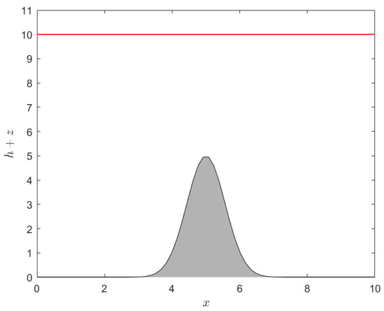
Figure 3. Water height at time $T=10$ s in Example 1.

Example 2

(Gaussian Pulse [13]). This example aims to demonstrate our method’s advantage in handling smooth solutions with reflecting boundary conditions over a flat bottom [13]. The initial Gaussian pulse for water height is defined by

$$h(x,0)=1+0.1exp\left\{-\left({\displaystyle \frac{x-0.5}{0.1}}\right)\right\}.$$

We simulated this experiment with $M=60$ grid points. The results from our numerical Algorithm 1 are shown in Figure 4. The wave consistently remained smooth. Initially, it separated into left and right propagating components, which then reflected off the walls and coalesced into a hump. This cycle continued over time, with the height gradually decreasing until the velocity approached zero, ultimately leading to a constant wave. This final state can be referred to as a steady state. Therefore, we observed that at time $T=9.5$, the experiment reached a steady state within a tolerance of ${10}^{-5}$ and with a run time of $8.6104$ min.

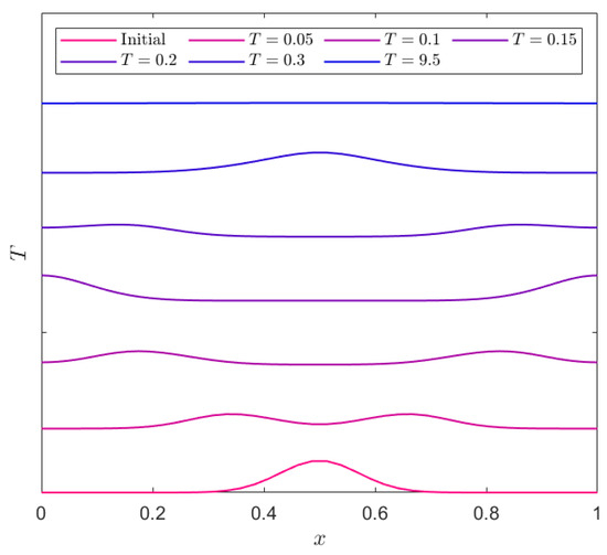
Figure 4. Water height $h(x,t)$ at various times T in Example 2.

Example 3

(Dam break over flat bottom [20]). This dam break problem is a fundamental study based on the SWEs, characterized by a flat topography where $z\left(x\right)=0$. The computational domain is $[0, 1]$. The initial velocity is zero and the initial water height is

$$h(x,0)=\left\{\begin{array}{cc}1\hfill & for0\le x<{\displaystyle \frac{1}{2}},\hfill \\ {\displaystyle \frac{1}{2}}\hfill & fofor{\displaystyle \frac{1}{2}}\le x\le 1.\hfill \end{array}\right.$$

This setup represents a discontinuity at $x={\displaystyle \frac{1}{2}}$, acting as a barrier separating two different initial water heights. The exact solution to this problem was provided by Stoker [20], specifically,

$$\begin{array}{cc}\hfill & h^{\ast }(x,t)=\left\{\begin{array}{cc}1\hfill & forx<{\displaystyle \frac{1}{2}}-t\sqrt{g},\hfill \\ {\displaystyle \frac{1}{9g}}{\left(2\sqrt{g}-{\displaystyle \frac{2x-1}{2t}}\right)}^2\hfill & for{\displaystyle \frac{1}{2}}-t\sqrt{g}\le x\le {\displaystyle \frac{1}{2}}+(v-w)t,\hfill \\ {\displaystyle \frac{w^2}{g}}\hfill & for{\displaystyle \frac{1}{2}}+(v-w)t<x\le {\displaystyle \frac{1}{2}}+St,\hfill \\ {\displaystyle \frac{1}{2}}\hfill & forx>{\displaystyle \frac{1}{2}}+St\hfill \end{array}\right.\hfill \end{array}$$

and

$$\begin{array}{c}{u}^{\ast }(x,t)=\left\{\begin{array}{cc}0\hfill & forx<{\displaystyle \frac{1}{2}}-t\sqrt{g},\hfill \\ {\displaystyle \frac{1}{3t}}{\left(2x-1+2t\sqrt{g}\right)}^2\hfill & for{\displaystyle \frac{1}{2}}-t\sqrt{g}\le x\le {\displaystyle \frac{1}{2}}+(v-w)t,\hfill \\ v\hfill & for{\displaystyle \frac{1}{2}}+(v-w)t<x{\displaystyle \frac{1}{2}}+St,\hfill \\ 0\hfill & forx>{\displaystyle \frac{1}{2}}+St,\hfill \end{array}\right.\hfill \end{array}$$

where $v=S-{\displaystyle \frac{g}{8S}}\left(1+\sqrt{1+{\displaystyle \frac{16S^2}{g}}}\right)$, $w=\sqrt{{\displaystyle \frac{g}{4}}\left(\sqrt{1+{\displaystyle \frac{16S^2}{g}}}-1\right)}$ and $S=2.9579181201875$. For a more in-depth analysis of how the value S was obtained, readers are referred to Stoker [20].

The numerical results obtained from our Algorithm 1 demonstrated good accuracy when compared with this exact solution. Comparisons, measured by the MAE from (25) at the final time T, are presented in Table 1 for different grid point values M. The error in Table 1 does not show a significant reduction as the grid is refined because the initial water height was discontinuous at $x={\displaystyle \frac{1}{2}}$. This discontinuity hindered the accurate capturing of the solution around the shock. Despite this, we further compared our algorithm’s approximate solutions with those obtained by the FDM [8] for various nodal points M, as shown in Table 1. It is evident that for the same number of nodes M, our scheme yielded solutions closer to the analytical solutions than the FDM. Additionally, increasing the number of nodes M generally led to increasingly accurate solutions. The computational times are also indicated in Table 1.

Table 1. Comparisons of exact and numerical solutions at $T=0.1$ for Example 3.

M	FDM [8]		Algorithm 1		Run Time (s)
	${\mathrm{MAE}}_{\mathit{h}}$	${\mathrm{MAE}}_{\mathit{u}}$	${\mathrm{MAE}}_{\mathit{h}}$	${\mathrm{MAE}}_{\mathit{u}}$
100	$2.02\times {10}^{-2}$	$7.53\times {10}^{-2}$	$4.73\times {10}^{-3}$	$1.65\times {10}^{-2}$	$0.4147$
200	$1.31\times {10}^{-2}$	$4.82\times {10}^{-2}$	$2.88\times {10}^{-3}$	$1.07\times {10}^{-2}$	$2.6712$
300	$9.96\times {10}^{-3}$	$3.64\times {10}^{-2}$	$2.05\times {10}^{-3}$	$7.72\times {10}^{-3}$	$8.4295$
400	$8.15\times {10}^{-3}$	$2.98\times {10}^{-2}$	$1.63\times {10}^{-3}$	$6.19\times {10}^{-3}$	$20.0024$

Furthermore, we visualized the solutions for both water height h and velocity u obtained using our algorithm with $M=200$ at $T=0.1$, as depicted in Figure 5. From Figure 5, the initial water height broke at $x={\displaystyle \frac{1}{2}}$ as time progressed. Our scheme effectively captured the shock propagation and showed good agreement with the exact solution.

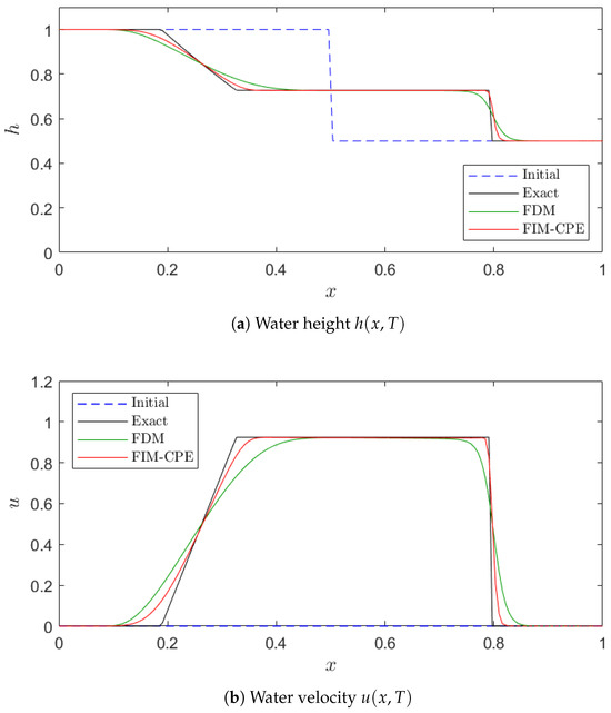
Figure 5. Graphical solutions with $M=200$ at time $T=0.1$ in Example 3.

Example 4

(Dam break over a bump [11]). This problem, discussed by LeVeque [11], involves a non-flat, smooth bottom topography, implying that $z^{\prime }\left(x\right)\ne 0$ for certain values of x. This test case features a smooth bump defined by

$$z\left(x\right)=\left\{\begin{array}{cc}{\displaystyle \frac{1}{4}}\left(\cos (10x-5)\pi +1\right)\hfill & \mathit{for}0.4\le x\le 0.6,\hfill \\ 0\hfill & \mathit{otherwise}.\hfill \end{array}\right.$$

The computational domain for this problem is $[0,1]$. The initial velocity is zero and the initial water height is defined in relation to the bump $z\left(x\right)$ as

$$h(x,0)=\left\{\begin{array}{cc}1-z\left(x\right)\hfill & \mathit{for}x<0.1,\hfill \\ {\displaystyle \frac{6}{5}}-z\left(x\right)\hfill & \mathit{for}0.1\le x\le 0.2,\hfill \\ 1-z\left(x\right)\hfill & \mathit{for}x>0.2.\hfill \end{array}\right.$$

This problem describes an initial water height shaped like a pulse that subsequently breaks into two waves propagating in opposite directions. The square-wave pulse moving towards the right passes through the bump in the riverbed, undergoing partial reflection and causing a disturbance behind the bump. The other wave reflects off the left wall.

In the experiment, our presented numerical Algorithm 1 was applied to find the approximate solutions for $h(x,t)$ and $u(x,t)$. Using $M=100$ grid points, we simulated the behavior of wave propagation at different times $t\in \{0.01,0.03,0.05,0.1,0.15,0.2\}$, as depicted in Figure 6 for water height and velocity. The run time for this simulation was $11.9876$ s. We observed that at the initial time, the wave pulse moved to the right, with $h+z$ around $1.1$. After the wave pulse encountered the bump, it was partially reflected, leading to a decrease in $h+z$ as it continued to move forward. Behind the bump, the wave pulse continued to decrease. The wave pulse also moved towards the left, with $h+z$ around $1.1$. After reaching the left wall, its height increased at $T=0.05$ and then returned to its previous level $T=0.1$. The behavior of the left wave was analogous to the right wave when passing the bump. This problem has also been studied using several methods by Hudson [8]. Our algorithm produced the same right wave behavior as those methods, given the reflection from the left wall.

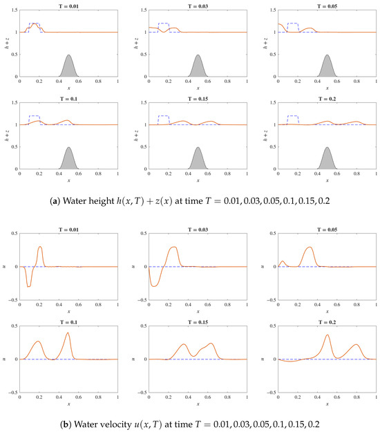
Figure 6. Graphical solutions for Example 4 (Dam break over a bump) with $M=100$ at different times T. (a) Water height $h(x,T)+z\left(x\right)$. The solid red line is the water surface, the dashed black line is the initial water surface and the gray area represents the bottom topography $z\left(x\right)$. (b) Water velocity $u(x,T)$. The solid red line is the water velocity and the dashed blue line indicates the zero-velocity axis.

3.4. Convergence Analysis

To numerically demonstrate the convergence of the proposed FIM-CPE scheme, a study was conducted to analyze the error decay as the spatial resolution increased. The dam break over a flat bottom (Example 3) was selected as the benchmark case for this analysis, due to the availability of an exact analytical solution.

The simulation was performed at a final time of $T=0.1$ s with an increasing number of Chebyshev nodes ($M_i)$. The MAE for the water height ($E_i$), as defined in (25), was calculated for each case. The results, presented in Table 2 and Figure 7, clearly illustrate the convergence of the solution.

Table 2. Convergence study for the dam break problem at $T=0.1$ s.

Index i	Number of Nodes    $\left({\mathit{M}}_{\mathit{i}}\right)$	MAE for Water Height $\left({\mathit{E}}_{\mathit{i}}\right)$	Order of Convergence $\left({\mathit{p}}_{\mathit{i}}\right)$
1	50	$7.6815\times {10}^{-3}$	-
2	100	$4.7312\times {10}^{-3}$	0.6992
3	200	$2.8839\times {10}^{-3}$	0.7142
4	400	$1.6271\times {10}^{-3}$	0.8257
5	800	$8.6563\times {10}^{-4}$	0.9105

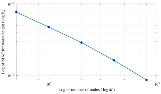
Figure 7. Log–log plot of the mean absolute error for water height (${\mathrm{MAE}}_h$) versus the number of nodes (M) for the dam break problem. The plot clearly shows the linear trend on a logarithmic scale, which demonstrates the convergence of the numerical scheme as the spatial resolution increases.

The numerical order of convergence ($p_i$) was calculated using the formula

$$p_i={\displaystyle \frac{log(E_{i-1}/E_i)}{log(M_i/M_{i-1})}},$$

where $E_{i-1}$ and $E_i$ are the errors corresponding to node counts $M_{i-1}$ and $M_i$, respectively. The order is approximately $0.7$–$0.9$. While spectral methods achieve higher orders for smooth problems, this result is consistent with expectations for problems involving a shock, where the overall accuracy is limited by the discontinuity.

The data in Table 2 and the trend in Figure 7 confirm that the error consistently decreased as the number of nodes increased, providing strong numerical evidence for the convergence of the FIM-CPE algorithm.

4. Two-Dimensional SWEs

This section presents a numerical method based on the FIM-CPE to solve the two-dimensional SWEs (2) with reflecting boundary conditions, as described in [13].

4.1. Numerical Algorithm for Two-Dimensional SWEs

Before deriving the algorithm, let $q_1=hu$ and $q_2=hv$ be the discharges. Then, (2) can be rewritten as

$$\begin{array}{c}\hfill \left\{\begin{array}{cc}\hfill & {\displaystyle \frac{\partial h}{\partial t}}+{\displaystyle \frac{\partial q_1}{\partial x}}+{\displaystyle \frac{\partial q_2}{\partial y}}=0,\hfill \\ \hfill & {\displaystyle \frac{\partial q_1}{\partial t}}+{\displaystyle \frac{\partial }{\partial x}}\left({\displaystyle \frac{q_1^2}{h}}+{\displaystyle \frac{g{h}^2}{2}}\right)+{\displaystyle \frac{\partial }{\partial y}}\left({\displaystyle \frac{q_1{q}_2}{h}}\right)+gh{\displaystyle \frac{\partial z}{\partial x}}=0,\hfill \\ \hfill & {\displaystyle \frac{\partial q_2}{\partial t}}+{\displaystyle \frac{\partial }{\partial x}}\left({\displaystyle \frac{q_1{q}_2}{h}}\right)+{\displaystyle \frac{\partial }{\partial y}}\left({\displaystyle \frac{q_2^2}{h}}+{\displaystyle \frac{g{h}^2}{2}}\right)+gh{\displaystyle \frac{\partial z}{\partial y}}=0,\hfill \end{array}\right.\end{array}$$

(26)

for all $(x,y,t)\in (a,b)\times (c,d)\times (0,T]$, where $a,b,c,d\in \mathbb{R}$ and $T\in {\mathbb{R}}^{+}$. We assume that h, u and v are smooth real-valued functions of the temporal coordinate. This system is subject to the initial conditions

$$h(x,y,0)={\varphi }_0(x,y),q_1(x,y,0)={\varphi }_1(x,y)\mathrm{and}{q}_2(x,y,0)={\varphi }_2(x,y)$$

(27)

for $(x,y)\in \Omega$, where $\Omega :=[a,b]\times [c,d]$ is the spatial domain. Let $\partial \Omega$ be the boundary of the domain $\Omega$. The reflecting boundary conditions [13] at any time $t\in (0,T]$ are given by

$$q_1(x,y,t)={\psi }_1(x,y)\mathrm{and}{q}_2(x,y,t)={\psi }_2(x,y)\mathrm{for}(x,y)\in \partial \Omega .$$

(28)

The FIM-CPE for two-dimensional SWEs employs procedures similar to those used for one-dimensional SWEs. Initially, the computational domain $(a,b)\times (c,d)$ is discretized into $H:=M\times N$ nodes. This is achieved by utilizing the zeros of the Chebyshev polynomials $R_M\left(x\right)$ and $R_N\left(x\right)$, as defined in (4), which denote them by $X:=\{x_1,x_2,x_3,\dots ,x_M\}$ and $Y:=\{y_1,y_2,y_3,\dots ,y_N\}$, respectively. The nodes are globally numbered and obtained from elements in the set of Cartesian product $X\times Y$, i.e., $(x_k,y_k)\in X\times Y$ for $k\in \{1,2,3,\dots ,H\}$. Concurrently, the temporal domain $(0,T]$ is divided into discrete time steps $t_{m+1}=t_m+\tau$ for all $m\in \mathbb{N}$, with $t_0=0$. The time step $\tau$ will be defined later.

Next, the time derivatives in the two-dimensional SWEs (26) are approximated using the first-order forward difference quotient. To manage the nonlinear terms effectively, a linearization method is applied. Consequently, the equations in (26) are transformed into

$$\begin{array}{cc}\hfill & {\displaystyle \frac{h^{⟨m+1⟩}-h^{⟨m⟩}}{\tau }}+{\displaystyle \frac{\partial q_1^{⟨m+1⟩}}{\partial x}}+{\displaystyle \frac{\partial q_2^{⟨m+1⟩}}{\partial y}}=0,\hfill \\ \hfill & {\displaystyle \frac{q_1^{⟨m+1⟩}-q_1^{⟨m⟩}}{\tau }}+{\displaystyle \frac{\partial }{\partial x}}\left({\displaystyle \frac{q_1^{⟨m⟩}{q}_1^{⟨m+1⟩}}{h^{⟨m⟩}}}+{\displaystyle \frac{g{h}^{⟨m⟩}{h}^{⟨m+1⟩}}{2}}\right)+{\displaystyle \frac{\partial }{\partial y}}\left({\displaystyle \frac{q_1^{⟨m⟩}{q}_2^{⟨m+1⟩}}{h^{⟨m⟩}}}\right)+g{h}^{⟨m+1⟩}{\displaystyle \frac{\partial z}{\partial x}}=0,\hfill \\ \hfill & {\displaystyle \frac{q_2^{⟨m+1⟩}-q_2^{⟨m⟩}}{\tau }}+{\displaystyle \frac{\partial }{\partial y}}\left({\displaystyle \frac{q_2^{⟨m⟩}{q}_2^{⟨m+1⟩}}{h^{⟨m⟩}}}+{\displaystyle \frac{g{h}^{⟨m⟩}{h}^{⟨m+1⟩}}{2}}\right)+{\displaystyle \frac{\partial }{\partial x}}\left({\displaystyle \frac{q_2^{⟨m⟩}{q}_1^{⟨m+1⟩}}{h^{⟨m⟩}}}\right)+g{h}^{⟨m+1⟩}{\displaystyle \frac{\partial z}{\partial y}}=0,\hfill \end{array}$$

where $h^{⟨m⟩}=h(x,y,t_m)$, $q_1^{⟨m⟩}=q_1(x,y,t_m)$ and $q_2^{⟨m⟩}=q_2(x,y,t_m)$ represent the numerical values at the m-th time step. Then, the water velocities are obtained by $u^{⟨m⟩}=q_1^{⟨m⟩}/h^{⟨m⟩}$ and $v^{⟨m⟩}=q_2^{⟨m⟩}/h^{⟨m⟩}$, respectively. To eliminate all derivatives, a double-layer integral with respect to the variables x and y is applied to both sides of the above system at time $t_m$. The integration is performed from a to $x_k$ and from c to $y_k$, respectively, yielding

$$\begin{array}{c}{\int }_c^{y_k}{\int }_a^{x_k}\left(h^{⟨m+1⟩}(\xi ,\eta )-h^{⟨m⟩}(\xi ,\eta )\right)d\xi d\eta \hfill \\ +\tau {\int }_c^{y_k}{q}_1^{⟨m+1⟩}(x_k,\eta )d\eta +\tau {\int }_a^{x_k}{q}_2^{⟨m+1⟩}(\xi ,y_k)d\xi +r_0\left(x_k\right)+s_0\left(y_k\right)=0,\end{array}$$

(29)

$$\begin{array}{c}{\int }_c^{y_k}{\int }_a^{x_k}\left(q_1^{⟨m+1⟩}(\xi ,\eta )-q_1^{⟨m⟩}(\xi ,\eta )\right)d\xi d\eta +\tau {\int }_c^{y_k}{u}^{⟨m⟩}(x_k,\eta )q_1^{⟨m+1⟩}(x_k,\eta )d\eta \hfill \\ +{\displaystyle \frac{\tau g}{2}}{\int }_c^{y_k}{h}^{⟨m⟩}(x_k,\eta )h^{⟨m+1⟩}(x_k,\eta )d\eta +\tau {\int }_a^{x_k}{u}^{⟨m⟩}(\xi ,y_k)q_2^{⟨m+1⟩}(\xi ,y_k)d\xi \hfill \\ +\tau g{\int }_c^{y_k}{\int }_a^{x_k}{\displaystyle \frac{\partial z(\xi ,\eta )}{\partial \xi }}{h}^{⟨m+1⟩}(\xi ,\eta )d\xi d\eta +r_1\left(x_k\right)+s_1\left(y_k\right)=0,\hfill \end{array}$$

(30)

$$\begin{array}{c}{\int }_c^{y_k}{\int }_a^{x_k}\left(q_2^{⟨m+1⟩}(\xi ,\eta )-q_2^{⟨m⟩}(\xi ,\eta )\right)d\xi d\eta +\tau {\int }_a^{x_k}{v}^{⟨m⟩}(\xi ,y_k)q_2^{⟨m+1⟩}(\xi ,y_k)d\xi \hfill \\ +{\displaystyle \frac{\tau g}{2}}{\int }_a^{x_k}{h}^{⟨m⟩}(\xi ,y_k)h^{⟨m+1⟩}(\xi ,y_k)d\xi +\tau {\int }_c^{y_k}{v}^{⟨m⟩}(x_k,\eta )q_1^{⟨m+1⟩}(x_k,\eta )d\eta \hfill \\ +\tau g{\int }_c^{y_k}{\int }_a^{x_k}{\displaystyle \frac{\partial z(\xi ,\eta )}{\partial \eta }}{h}^{⟨m+1⟩}(\xi ,\eta )d\xi d\eta +r_2\left(x_k\right)+s_2\left(y_k\right)=0,\hfill \end{array}$$

(31)

where $r_i\left(x_k\right)$ and $s_i\left(y_k\right)$ for $i\in \{0,1,2\}$ are arbitrary functions introduced during the integration process. To handle these unknown functions, Chebyshev interpolation is used to approximate them by

$$\begin{array}{cc}\hfill r_i\left(x\right)& =\sum _{n=0}^{M-1}{r}_{i,n}{R}_n\left(x\right)\mathrm{for}i\in \{0,1,2\}\mathrm{and}\hfill \end{array}$$

(32)

$$\begin{array}{cc}\hfill s_i\left(y\right)& =\sum _{n=0}^{N-1}{s}_{i,n}{R}_n\left(y\right)\mathrm{for}i\in \{0,1,2\},\hfill \end{array}$$

(33)

where ${\left\{r_{i,n}\right\}}_{n=0}^{M-1}$ and ${\left\{s_{i,n}\right\}}_{n=0}^{N-1}$ are unknown coefficients that will be determined according to the specified boundary conditions (28). Note that the total number of these unknown coefficients is ${\sum }_{i=0}^2(M+N)=3M+3N$.

Subsequently, each of the Equations (29)–(31) is rearranged into matrix form using the Chebyshev integration matrix. By substituting all zeros $(x_k,y_k),k\in \{1,2,3,\dots ,H\}$ into these equations, the following matrix equations are obtained:

$${\mathbf{A}}_x{\mathbf{A}}_y{\mathbf{h}}^{⟨m+1⟩}+\tau {\mathbf{A}}_y{\mathbf{q}}_1^{⟨m+1⟩}+\tau {\mathbf{A}}_x{\mathbf{q}}_2^{⟨m+1⟩}+{\mathsf{\Phi }}_x{\mathbf{r}}_0+{\mathsf{\Phi }}_y{\mathbf{s}}_0={\mathbf{A}}_x{\mathbf{A}}_y{\mathbf{h}}^{⟨m⟩},$$

(34)

$$\begin{array}{c}{\mathbf{A}}_x{\mathbf{A}}_y{\mathbf{q}}_1^{⟨m+1⟩}+\tau {\mathbf{A}}_y{\mathbf{U}}^{⟨m⟩}{\mathbf{q}}_1^{⟨m+1⟩}+{\displaystyle \frac{\tau g}{2}}{\mathbf{A}}_y{\mathbf{H}}^{⟨m⟩}{\mathbf{h}}^{⟨m+1⟩}\hfill \\ +\tau {\mathbf{A}}_x{\mathbf{U}}^{⟨m⟩}{\mathbf{q}}_2^{⟨m+1⟩}+\tau g{\mathbf{A}}_x{\mathbf{A}}_y{\mathbf{Z}}_x{\mathbf{h}}^{⟨m+1⟩}+{\mathsf{\Phi }}_x{\mathbf{r}}_1+{\mathsf{\Phi }}_y{\mathbf{s}}_1={\mathbf{A}}_x{\mathbf{A}}_y{\mathbf{q}}_1^{⟨m⟩},\hfill \end{array}$$

(35)

$$\begin{array}{c}{\mathbf{A}}_x{\mathbf{A}}_y{\mathbf{q}}_2^{⟨m+1⟩}+\tau {\mathbf{A}}_x{\mathbf{V}}^{⟨m⟩}{\mathbf{q}}_2^{⟨m+1⟩}+{\displaystyle \frac{\tau g}{2}}{\mathbf{A}}_x{\mathbf{H}}^{⟨m⟩}{\mathbf{h}}^{⟨m+1⟩}\hfill \\ +\tau {\mathbf{A}}_y{\mathbf{V}}^{⟨m⟩}{\mathbf{q}}_1^{⟨m+1⟩}+\tau g{\mathbf{A}}_x{\mathbf{A}}_y{\mathbf{Z}}_y{\mathbf{h}}^{⟨m+1⟩}+{\mathsf{\Phi }}_x{\mathbf{r}}_2+{\mathsf{\Phi }}_y{\mathbf{s}}_2={\mathbf{A}}_x{\mathbf{A}}_y{\mathbf{q}}_2^{⟨m⟩},\hfill \end{array}$$

(36)

where ${\mathbf{A}}_x$ and ${\mathbf{A}}_y$ are the two-dimensional Chebyshev integration matrices along the x-axis and y-axis, respectively, described in Section 2.2. Other parameters in the system (34)–(36) are defined by

$$\begin{array}{ccc}{\mathbf{h}}^{⟨m⟩}\hfill & =& {\left[h^{⟨m⟩}(x_1,y_1),h^{⟨m⟩}(x_2,y_2),h^{⟨m⟩}(x_3,y_3),\dots ,h^{⟨m⟩}(x_H,y_H)\right]}^{\top },\hfill \\ {\mathbf{q}}_1^{⟨m⟩}\hfill & =& {\left[q_1^{⟨m⟩}(x_1,y_1),q_1^{⟨m⟩}(x_2,y_2),q_1^{⟨m⟩}(x_3,y_3),\dots ,q_1^{⟨m⟩}(x_H,y_H)\right]}^{\top },\hfill \\ {\mathbf{q}}_2^{⟨m⟩}\hfill & =& {\left[q_2^{⟨m⟩}(x_1,y_1),q_2^{⟨m⟩}(x_2,y_2),q_2^{⟨m⟩}(x_3,y_3),\dots ,q_2^{⟨m⟩}(x_H,y_H)\right]}^{\top },\hfill \\ {\mathbf{H}}^{⟨m⟩}\hfill & =& \mathrm{diag}\left\{h^{⟨m⟩}(x_1,y_1),h^{⟨m⟩}(x_2,y_2),h^{⟨m⟩}(x_3,y_3),\dots ,h^{⟨m⟩}(x_H,y_H)\right\},\hfill \\ {\mathbf{U}}^{⟨m⟩}\hfill & =& \mathrm{diag}\left\{u^{⟨m⟩}(x_1,y_1),u^{⟨m⟩}(x_2,y_2),u^{⟨m⟩}(x_3,y_3),\dots ,u^{⟨m⟩}(x_H,y_H)\right\},\hfill \\ {\mathbf{V}}^{⟨m⟩}\hfill & =& \mathrm{diag}\left\{v^{⟨m⟩}(x_1,y_1),v^{⟨m⟩}(x_2,y_2),v^{⟨m⟩}(x_3,y_3),\dots ,v^{⟨m⟩}(x_H,y_H)\right\},\hfill \\ {\mathbf{Z}}_x\hfill & =& \mathrm{diag}\left\{z_x(x_1,y_1),z_x(x_2,y_2),z_x(x_3,y_3),\dots ,z_x(x_H,y_H)\right\},\hfill \\ {\mathbf{Z}}_y\hfill & =& \mathrm{diag}\left\{z_y(x_1,y_1),z_y(x_2,y_2),z_y(x_3,y_3),\dots ,z_y(x_H,y_H)\right\},\hfill \\ {\mathbf{r}}_i\hfill & =& {\left[r_{i,0},r_{i,1},r_{i,2},\dots ,r_{i,M-1}\right]}^{\top }\mathrm{for}i\in \{0,1,2\}\mathrm{and}\hfill \\ {\mathbf{s}}_i\hfill & =& {\left[s_{i,0},s_{i,1},s_{i,2},\dots ,s_{i,N-1}\right]}^{\top }\mathrm{for}i\in \{0,1,2\}.\hfill \end{array}$$

From (32) and (33), we have their coefficient matrices as

$${\mathsf{\Phi }}_x=\left[\begin{array}{cccc}{R}_0\left(x_1\right)& R_1\left(x_1\right)& \cdots & R_{M-1}\left(x_1\right)\\ R_0\left(x_2\right)& R_1\left(x_2\right)& \cdots & R_{M-1}\left(x_2\right)\\ ⋮& ⋮& \ddots & ⋮\\ R_0\left(x_H\right)& R_1\left(x_H\right)& \cdots & R_{M-1}\left(x_H\right)\end{array}\right]$$

and

$${\mathsf{\Phi }}_y=\left[\begin{array}{cccc}{R}_0\left(y_1\right)& R_1\left(y_1\right)& \cdots & R_{N-1}\left(y_1\right)\\ R_0\left(y_2\right)& R_1\left(y_2\right)& \cdots & R_{N-1}\left(y_2\right)\\ ⋮& ⋮& \ddots & ⋮\\ R_0\left(y_H\right)& R_1\left(y_H\right)& \cdots & R_{N-1}\left(y_H\right)\end{array}\right].$$

Since the integral system (29)–(31) incorporates the additional $3M+3N$ unknown coefficients denoted as $r_{i,n}$ and $s_{i,n}$, it is necessary to generate an extra $3M+3N$ equations, derived from the rectangular boundary conditions given by (28). For the boundary condition on $q_1$, this approach involves formulating M equations from its left boundary, N equations from its lower boundary, $\lceil {\displaystyle \frac{M}{2}}\rceil$ equations from its right boundary, and $\lceil {\displaystyle \frac{N}{2}}\rceil$ equations from its upper boundary. Specifically, over the right and upper boundaries of $q_1$, these additional equations are constructed at the zero points of Chebyshev polynomials that are indexed in odd positions, as depicted in Figure 8a.

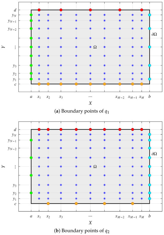
Figure 8. The selected computational nodes for the 2D problem. The blue asterisks (*) represent the interior nodes within the domain $\Omega$. The colored dots represent the nodes on the boundary $\partial \Omega$ where boundary conditions are applied: orange for the bottom, green for the left, red for the top, and cyan for the right. (a) The specific set of boundary points used to enforce conditions for the discharge $q_1$. (b) The complementary set of boundary points used for the discharge $q_2$.

Conversely, the boundary condition on $q_2$ requires constructing M equations from its right boundary, N equations from its upper boundary, $\lfloor {\displaystyle \frac{M}{2}}\rfloor$ equations from its left boundary, and $\lfloor {\displaystyle \frac{N}{2}}\rfloor$ equations from its lower boundary. In particular, over the left and lower boundaries of $q_2$, these equations are constructed at the zero points of Chebyshev polynomials that are indexed in even positions, as depicted in Figure 8b.

Afterward, these specified boundary conditions (28) are converted into matrix form using Theorem 2, which extends the one-dimensional Chebyshev polynomial expansion (5) to two dimensions, as described below.

Theorem 2.

Let $X:=\{x_1,x_2,x_3,\dots ,x_M\}\subseteq (a,b)$ and $Y:=\{y_1,y_2,y_3,\dots ,y_N\}\subseteq (c,d)$ be sets of zeros of the Chebyshev polynomials $R_M\left(x\right)$ and $R_N\left(y\right)$, respectively. If f is a function of x and y on $[a,b]\times [c,d]\subseteq {\mathbb{R}}^2$, it can be approximated at any $x\in [a, b]$ or $y\in [c, d]$ by the Chebyshev polynomial expansion in the matrix form as

$$\begin{array}{cc}\hfill \mathbf{f}(x,·)& =\left({\mathbf{I}}_N\otimes {\mathit{\rho }}_x^{\top }{\mathbf{R}}_M^{-1}\right)\mathbf{f}and\hfill \end{array}$$

(37)

$$\begin{array}{cc}\hfill \mathbf{f}(·,y)& =\left({\mathbf{I}}_M\otimes {\mathit{\rho }}_y^{\top }{\mathbf{R}}_N^{-1}\right){\mathbf{P}}^{-1}\mathbf{f}\hfill \end{array}$$

(38)

where ${\mathit{\rho }}_x={[R_0\left(x\right),R_1\left(x\right),R_2\left(x\right),\dots ,R_{M-1}\left(x\right)]}^{\top }$, ${\mathit{\rho }}_y={[R_0\left(y\right),R_1\left(y\right),R_2\left(y\right),\dots ,R_{N-1}\left(y\right)]}^{\top }$, ${\mathbf{R}}_M$ and ${\mathbf{R}}_N$ are the $M\times M$ and $N\times N$ Chebyshev matrices, respectively, defined in Lemma 1(iii) and $\mathbf{f}={[f(x_1,y_1),f(x_2,y_2),f(x_3,y_3),\dots ,f(x_{MN},y_{MN})]}^{\top }$ with elements ordered according to a global numbering system for the grid points $(x_k,y_k)$ belong to the set of Cartesian product $X\times Y$. Other parameters are as defined in Section 2.2.

Proof of Theorem 2.

We consider a function $f(x,y)$ expressed as a Chebyshev polynomial expansion (5). By holding one variable constant while varying the other, the proof is structured into two scenarios:

• Scenario I: When y is held constant and x is the free variable, we have

  $$f(x,y)=\sum _{n=0}^{M-1}{c}_{f,n}{R}_n\left(x\right):={\mathit{\rho }}_x^{\top }{\mathbf{c}}_f={\mathit{\rho }}_x^{\top }{\mathbf{R}}_M^{-1}\mathbf{f}(·,y),$$

  (39)

  where ${\mathit{\rho }}_x={[R_0\left(x\right),R_1\left(x\right),R_2\left(x\right),\dots ,R_{M-1}\left(x\right)]}^{\top }$, ${\mathbf{R}}_M$ is an $M\times M$ Chebyshev matrix as defined in Lemma 1(iii) and $\mathbf{f}(·,y)={[f(x_1,y),f(x_2,y),f(x_3,y),\dots ,f(x_M,y)]}^{\top }$. Substituting the zeros of the Chebyshev polynomial $R_N\left(y\right)$, i.e., $y\in \{y_1,y_2,y_3,\dots ,y_N\}$, into (39) yields

  $$\left[\begin{array}{c}f(x,y_1)\\ f(x,y_2)\\ ⋮\\ f(x,y_N)\end{array}\right]=\underset{N\mathrm{blocks}}{\underbrace{\left[\begin{array}{cccc}{\mathit{\rho }}_x^{\top }{\mathbf{R}}_M^{-1}& 0& \cdots & 0\\ 0& {\mathit{\rho }}_x^{\top }{\mathbf{R}}_M^{-1}& \ddots & ⋮\\ ⋮& \ddots & \ddots & 0\\ 0& \cdots & 0& {\mathit{\rho }}_x^{\top }{\mathbf{R}}_M^{-1}\end{array}\right]}}\left[\begin{array}{c}\mathbf{f}(·,y_1)\\ \mathbf{f}(·,y_2)\\ ⋮\\ \mathbf{f}(·,y_N)\end{array}\right].$$
  This simplifies to $\mathbf{f}(x,·)=\left({\mathbf{I}}_N\otimes {\mathit{\rho }}_x^{\top }{\mathbf{R}}_M^{-1}\right)\mathbf{f}$, where ${\mathbf{I}}_N$ is an $N\times N$ identity matrix.
• Scenario II: When x is held constant and y is the free variable, we have

  $$f(x,y)=\sum _{n=0}^{N-1}{c}_{f,n}{R}_n\left(y\right):={\mathit{\rho }}_y^{\top }{\mathbf{c}}_f={\mathit{\rho }}_y^{\top }{\mathbf{R}}_N^{-1}\mathbf{f}(x,·),$$

  (40)

  where ${\mathit{\rho }}_y={[R_0\left(y\right),R_1\left(y\right),R_2\left(y\right),\dots , R_{N-1}\left(y\right)]}^{\top }$, ${\mathbf{R}}_M$ is an $N\times N$ Chebyshev matrix as defined in Lemma 1(iii) and $\mathbf{f}(x, ·)={[f(x, y_1),f(x, y_2),f(x, y_3),\dots , f(x, y_N)]}^{\top }$. Substituting the zeros of the Chebyshev polynomial $R_M\left(x\right)$, i.e., $x\in \{x_1, x_2, x_3,\dots , x_M\}$, into (40) yields

  $$\left[\begin{array}{c}f(x_1,y)\\ f(x_2,y)\\ ⋮\\ f(x_M,y)\end{array}\right]=\underset{M\mathrm{blocks}}{\underbrace{\left[\begin{array}{cccc}{\mathit{\rho }}_y^{\top }{\mathbf{R}}_N^{-1}& 0& \cdots & 0\\ 0& {\mathit{\rho }}_y^{\top }{\mathbf{R}}_N^{-1}& \ddots & ⋮\\ ⋮& \ddots & \ddots & 0\\ 0& \cdots & 0& {\mathit{\rho }}_y^{\top }{\mathbf{R}}_N^{-1}\end{array}\right]}}\left[\begin{array}{c}\mathbf{f}(x_1,·)\\ \mathbf{f}(x_2,·)\\ ⋮\\ \mathbf{f}(x_M,·)\end{array}\right].$$
  This simplifies to $\mathbf{f}(·, y)=\left({\mathbf{I}}_M\otimes {\mathit{\rho }}_y^{\top }{\mathbf{R}}_N^{-1}\right)\tilde{\mathbf{f}}=\left({\mathbf{I}}_M\otimes {\mathit{\rho }}_y^{\top }{\mathbf{R}}_N^{-1}\right){\mathbf{P}}^{-1}\mathbf{f}$, where ${\mathbf{I}}_M$ is an $M\times M$ identity matrix and $\mathbf{P}$ is a permutation matrix defined by (10).

Hence, the proof is complete.    □

Utilizing Theorem 2 and the boundary conditions (28) at time $t_{m+1}$, we directly derive four boundary conditions (41)–(44) in matrix form by substituting $q_i^{⟨m+1⟩}$ for f in Theorem 2 and evaluating at the respective boundary points, as follows:

• The left and lower boundary conditions for $q_1={\psi }_1(x, y)$ at time $t_{m+1}$ are obtained by replacing $x=a$ and $y=c$ into (37) and (38), respectively:

  $$\begin{array}{cc}\hfill {\mathbf{q}}_1^{⟨m+1⟩}(a,·)& =\left({\mathbf{I}}_N\otimes {\mathit{\rho }}_a^{\top }{\mathbf{R}}_M^{-1}\right){\mathbf{q}}_1^{⟨m+1⟩}:={\Psi }_{1a}\mathrm{and}\hfill \end{array}$$

  (41)

  $$\begin{array}{cc}\hfill {\mathbf{q}}_1^{⟨m+1⟩}(·,c)& =\left({\mathbf{I}}_M\otimes {\mathit{\rho }}_c^{\top }{\mathbf{R}}_N^{-1}\right){\mathbf{P}}^{-1}{\mathbf{q}}_1^{⟨m+1⟩}:={\Psi }_{1c},\hfill \end{array}$$

  (42)

  where ${\mathit{\rho }}_a={[1,-1,1,-1,\dots ,{(-1)}^{M-1}]}^{\top }$, ${\Psi }_{1a}={[{\psi }_1(a,y_1),{\psi }_1(a,y_2),\dots ,{\psi }_1(a,y_N)]}^{\top }$, ${\mathit{\rho }}_c={[1,-1,1,-1,\dots ,{(-1)}^{N-1}]}^{\top }$ and ${\Psi }_{1c}={[{\psi }_1(x_1,c),{\psi }_1(x_2,c),\dots ,{\psi }_1(x_M,c)]}^{\top }$.
• The right and upper boundary conditions for $q_2={\psi }_2(x,y)$ at time $t_{m+1}$ are obtained by replacing $x=b$ and $y=d$ into (37) and (38), respectively:

  $$\begin{array}{cc}\hfill {\mathbf{q}}_2^{⟨m+1⟩}(b,·)& =\left({\mathbf{I}}_N\otimes {\mathit{\rho }}_b^{\top }{\mathbf{R}}_M^{-1}\right){\mathbf{q}}_2^{⟨m+1⟩}:={\Psi }_{2b}\mathrm{and}\hfill \end{array}$$

  (43)

  $$\begin{array}{cc}\hfill {\mathbf{q}}_2^{⟨m+1⟩}(·,d)& =\left({\mathbf{I}}_M\otimes {\mathit{\rho }}_d^{\top }{\mathbf{R}}_N^{-1}\right){\mathbf{P}}^{-1}{\mathbf{q}}_2^{⟨m+1⟩}:={\Psi }_{2d},\hfill \end{array}$$

  (44)

  where ${\mathit{\rho }}_b={[1,1,1,\dots ,1]}^{\top }$ with M entries, ${\Psi }_{2b}={[{\psi }_2(b,y_1),{\psi }_2(b,y_2),\dots ,{\psi }_2(b,y_N)]}^{\top }$, ${\mathit{\rho }}_d={[1,1,1,\dots ,1]}^{\top }$ with N entries and ${\Psi }_{2d}={[{\psi }_2(x_1,d),{\psi }_2(x_2,d),\dots ,{\psi }_2(x_M,d)]}^{\top }$.

Next, we address the boundary conditions for the remaining sides involving $q_1$ and $q_2$. To handle boundary conditions that depend on the parity of index positions (odd or even), we introduce an extraction matrix. An extraction matrix multiplies a column vector to yield a new column vector composed of selected entries from the original. In this work, we define two types of extraction matrices—odd and even—in Definition 3, which select entries from corresponding positions in a column vector.

Definition 3.

The odd extraction matrix, denoted by ${\mathbf{T}}_{\mathrm{odd}}={\left[a_{ij}\right]}_{m\times n}$, is defined as

$$\begin{array}{cc}\hfill a_{ij}& =\left\{\begin{array}{cc}1\hfill & ;j=2i-1\mathit{and}i\in \{1,2,3,\dots ,m\},\hfill \\ 0\hfill & ;\mathit{otherwise}.\hfill \end{array}\right.\hfill \end{array}$$

(45)

Moreover, the even extraction matrix, denoted by ${\mathbf{T}}_{\mathrm{even}}={\left[b_{ij}\right]}_{m\times n}$, is defined as

$$\begin{array}{cc}\hfill b_{ij}& =\left\{\begin{array}{cc}1\hfill & ;j=2i\mathit{and}i\in \{1,2,3,\dots ,m\},\hfill \\ 0\hfill & ;\mathit{otherwise}.\hfill \end{array}\right.\hfill \end{array}$$

(46)

Building upon Definition 3, Theorem 2 and the boundary conditions (28) at time $t_{m+1}$, the remaining boundary conditions for $q_1$ and $q_2$ are formulated as follows:

• The right and upper boundary conditions for $q_1={\psi }_1(x,y)$ at time $t_{m+1}$ over the odd position corresponding to $\lceil {\displaystyle \frac{M}{2}}\rceil$ and $\lceil {\displaystyle \frac{N}{2}}\rceil$ zeros in X and Y, respectively, are obtained by substituting $x=b$ and $y=d$ into (37) and (38), respectively, and left-multiplying by ${\mathbf{T}}_{\mathrm{odd}}$ from (45):

  $${\mathbf{T}}_{\mathrm{odd}}^x{\mathbf{q}}_1^{⟨m+1⟩}(b,·)={\mathbf{T}}_{\mathrm{odd}}^x\left({\mathbf{I}}_N\otimes {\mathit{\rho }}_b^{\top }{\mathbf{R}}_M^{-1}\right){\mathbf{q}}_1^{⟨m+1⟩}:={\mathbf{T}}_{\mathrm{odd}}^x{\Psi }_{1b}\mathrm{and}$$

  (47)

  $${\mathbf{T}}_{\mathrm{odd}}^y{\mathbf{q}}_1^{⟨m+1⟩}(·,d)={\mathbf{T}}_{\mathrm{odd}}^y\left({\mathbf{I}}_M\otimes {\mathit{\rho }}_d^{\top }{\mathbf{R}}_N^{-1}\right){\mathbf{P}}^{-1}{\mathbf{q}}_1^{⟨m+1⟩}:={\mathbf{T}}_{\mathrm{odd}}^y{\Psi }_{1d},$$

  (48)

  where ${\mathbf{T}}_{\mathrm{odd}}^x$ is an $\lceil {\displaystyle \frac{M}{2}}\rceil \times M$ odd extraction, ${\Psi }_{1b}={[{\psi }_1(b,y_1),{\psi }_1(b,y_2),\dots ,{\psi }_1(b,y_N)]}^{\top }$, ${\mathbf{T}}_{\mathrm{odd}}^y$ is an $\lceil {\displaystyle \frac{N}{2}}\rceil \times N$ odd extraction, and ${\Psi }_{1d}={[{\psi }_1(x_1,d),{\psi }_1(x_2,d),\dots ,{\psi }_1(x_M,d)]}^{\top }$.
• The left and lower boundary conditions for $q_2={\psi }_2(x,y)$ at time $t_{m+1}$ over the even positions corresponding to $\lfloor {\displaystyle \frac{M}{2}}\rfloor$ and $\lfloor {\displaystyle \frac{N}{2}}\rfloor$ zeros in X and Y, respectively, are obtained by replacing $x=a$ and $y=c$ into (37) and (38), respectively, and left-multiplying by ${\mathbf{T}}_{\mathrm{even}}$ from (46):

  $${\mathbf{T}}_{\mathrm{even}}^x{\mathbf{q}}_2^{⟨m+1⟩}(a,·)={\mathbf{T}}_{\mathrm{even}}^x\left({\mathbf{I}}_N\otimes {\mathit{\rho }}_a^{\top }{\mathbf{R}}_M^{-1}\right){\mathbf{q}}_2^{⟨m+1⟩}:={\mathbf{T}}_{\mathrm{even}}^x{\Psi }_{2a}\mathrm{and}$$

  (49)

  $${\mathbf{T}}_{\mathrm{even}}^y{\mathbf{q}}_2^{⟨m+1⟩}(·,c)={\mathbf{T}}_{\mathrm{even}}^y\left({\mathbf{I}}_M\otimes {\mathit{\rho }}_c^{\top }{\mathbf{R}}_N^{-1}\right){\mathbf{P}}^{-1}{\mathbf{q}}_2^{⟨m+1⟩}:={\mathbf{T}}_{\mathrm{even}}^y{\Psi }_{2c},$$

  (50)

  where ${\mathbf{T}}_{\mathrm{even}}^x$ is an $\lfloor {\displaystyle \frac{M}{2}}\rfloor \times M$ even extraction, ${\Psi }_{2a}={[{\psi }_2(a,y_1),{\psi }_2(a,y_2),\dots ,{\psi }_2(a,y_N)]}^{\top }$, ${\mathbf{T}}_{\mathrm{even}}^y$ is an $\lfloor {\displaystyle \frac{N}{2}}\rfloor \times N$ even extraction, and ${\Psi }_{2c}={[{\psi }_2(x_1,c),{\psi }_2(x_2,c),\dots ,{\psi }_2(x_M,c)]}^{\top }$.

Finally, the systems (34–36) and boundary conditions (41)–(44) and (47)–(50) are combined to form a system of linear equations. It comprises a total of $3H+3M+3N$ unknowns, namely ${\mathbf{h}}^{⟨m+1⟩}$, ${\mathbf{q}}_1^{⟨m+1⟩},{\mathbf{q}}_2^{⟨m+1⟩}$, ${\mathbf{r}}_0$, ${\mathbf{s}}_0$, ${\mathbf{r}}_1$, ${\mathbf{s}}_1$, ${\mathbf{r}}_2$, and ${\mathbf{s}}_2$. The resulting system is

$$\left[\begin{array}{cccccc}{\mathbf{A}}_x{\mathbf{A}}_y& \tau {\mathbf{A}}_y& \tau {\mathbf{A}}_x& [{\mathsf{\Phi }}_x,{\mathsf{\Phi }}_y]& {\mathbf{0}}_{H\times L}& {\mathbf{0}}_{H\times L}\\ \tau g{\mathbf{A}}_y({\displaystyle \frac{1}{2}}{\mathbf{H}}^{⟨m⟩}+{\mathbf{A}}_x{\mathbf{Z}}_x)& {\mathbf{A}}_y({\mathbf{A}}_x+\tau {\mathbf{U}}^{⟨m⟩})& \tau {\mathbf{A}}_x{\mathbf{U}}^{⟨m⟩}& {\mathbf{0}}_{H\times L}& [{\mathsf{\Phi }}_x,{\mathsf{\Phi }}_y]& {\mathbf{0}}_{H\times L}\\ \tau g{\mathbf{A}}_x({\displaystyle \frac{1}{2}}{\mathbf{H}}^{⟨m⟩}+{\mathbf{A}}_y{\mathbf{Z}}_y)& \tau {\mathbf{A}}_y{\mathbf{V}}^{⟨m⟩}& {\mathbf{A}}_x({\mathbf{A}}_y+\tau {\mathbf{V}}^{⟨m⟩})& {\mathbf{0}}_{H\times L}& {\mathbf{0}}_{H\times L}& [{\mathsf{\Phi }}_x,{\mathsf{\Phi }}_y]\\ {\mathbf{0}}_{N\times H}& {\mathbf{W}}_x\left(a\right)& {\mathbf{0}}_{N\times H}\\ {\mathbf{0}}_{M\times H}& {\mathbf{W}}_y\left(c\right)& {\mathbf{0}}_{M\times H}\\ {\mathbf{0}}_{N\times H}& {\mathbf{0}}_{N\times H}& {\mathbf{W}}_x\left(b\right)\\ {\mathbf{0}}_{M\times H}& {\mathbf{0}}_{M\times H}& {\mathbf{W}}_y\left(d\right)\\ {\mathbf{0}}_{\lceil {\displaystyle \frac{N}{2}}\rceil \times H}& {\mathbf{T}}_{\mathrm{odd}}^x{\mathbf{W}}_x\left(b\right)& {\mathbf{0}}_{\lceil {\displaystyle \frac{N}{2}}\rceil \times H}& & {\mathbf{0}}_{3L\times 3L}& \\ {\mathbf{0}}_{\lceil {\displaystyle \frac{M}{2}}\rceil \times H}& {\mathbf{T}}_{\mathrm{odd}}^y{\mathbf{W}}_y\left(d\right)& {\mathbf{0}}_{\lceil {\displaystyle \frac{M}{2}}\rceil \times H}\\ {\mathbf{0}}_{\lfloor {\displaystyle \frac{N}{2}}\rfloor \times H}& {\mathbf{0}}_{\lfloor {\displaystyle \frac{N}{2}}\rfloor \times H}& {\mathbf{T}}_{\mathrm{even}}^x{\mathbf{W}}_x\left(a\right)\\ {\mathbf{0}}_{\lfloor {\displaystyle \frac{M}{2}}\rfloor \times H}& {\mathbf{0}}_{\lfloor {\displaystyle \frac{M}{2}}\rfloor \times H}& {\mathbf{T}}_{\mathrm{even}}^y{\mathbf{W}}_x\left(c\right)\end{array}\right]\left[\begin{array}{c}{\mathbf{h}}^{⟨m+1⟩}\\ {\mathbf{q}}_1^{⟨m+1⟩}\\ {\mathbf{q}}_2^{⟨m+1⟩}\\ {\mathbf{r}}_0\\ {\mathbf{s}}_0\\ {\mathbf{r}}_1\\ {\mathbf{s}}_1\\ {\mathbf{r}}_2\\ {\mathbf{s}}_2\end{array}\right]=\left[\begin{array}{c}\mathbf{A}{\mathbf{h}}^{⟨m⟩}\\ \mathbf{A}{\mathbf{q}}_1^{⟨m⟩}\\ \mathbf{A}{\mathbf{q}}_2^{⟨m⟩}\\ {\Psi }_{1a}\\ {\Psi }_{1c}\\ {\Psi }_{2b}\\ {\Psi }_{2d}\\ {\mathbf{T}}_{\mathrm{odd}}^x{\Psi }_{1b}\\ {\mathbf{T}}_{\mathrm{odd}}^y{\Psi }_{1d}\\ {\mathbf{T}}_{\mathrm{even}}^x{\Psi }_{2a}\\ {\mathbf{T}}_{\mathrm{even}}^y{\Psi }_{2c}\end{array}\right],$$

(51)

where $L=M+N$, ${\mathbf{W}}_x\left(\lambda \right)={\mathbf{I}}_N\otimes {\mathit{\rho }}_{\lambda }^{\top }{\mathbf{R}}_M^{-1}$ and ${\mathbf{W}}_y\left(\lambda \right)=({\mathbf{I}}_M\otimes {\mathit{\rho }}_{\lambda }^{\top }{\mathbf{R}}_N^{-1}){\mathbf{P}}^{-1}$ for $\lambda \in \{a,b,c,d\}$. This system (51) is subsequently solved to obtain the approximate solutions ${\mathbf{h}}^{⟨m+1⟩}$, ${\mathbf{q}}_1^{⟨m+1⟩}$ and ${\mathbf{q}}_2^{⟨m+1⟩}$. The solution process commences with the initial conditions (27) expressed in vector form:

$$\begin{array}{cc}\hfill {\mathbf{h}}^{⟨0⟩}& ={[{\varphi }_0(x_1,y_1),{\varphi }_0(x_2,y_2),{\varphi }_0(x_3,y_3),\dots ,{\varphi }_0(x_H,,y_H)]}^{\top },\hfill \\ \hfill {\mathbf{q}}_1^{⟨0⟩}& ={[{\varphi }_1(x_1,y_1),{\varphi }_1(x_2,y_2),{\varphi }_1(x_3,y_3),\dots ,{\varphi }_1(x_H,,y_H)]}^{\top },\hfill \\ \hfill {\mathbf{q}}_2^{⟨0⟩}& ={[{\varphi }_2(x_1,y_1),{\varphi }_2(x_2,y_2),{\varphi }_2(x_3,y_3),\dots ,{\varphi }_2(x_H,,y_H)]}^{\top },\hfill \\ \hfill {\mathbf{u}}^{⟨0⟩}& ={\mathbf{q}}_1^{⟨0⟩}\oslash {\mathbf{h}}^{⟨0⟩}\mathrm{and}{\mathbf{v}}^{⟨0⟩}={\mathbf{q}}_2^{⟨0⟩}\oslash {\mathbf{h}}^{⟨0⟩}.\hfill \end{array}$$

Therefore, the solutions for velocity components ${\mathbf{u}}^{⟨m+1⟩}$ and ${\mathbf{v}}^{⟨m+1⟩}$ are directly obtained by ${\mathbf{u}}^{⟨m+1⟩}={\mathbf{q}}_1^{⟨m+1⟩}\oslash {\mathbf{h}}^{⟨m+1⟩}$ and ${\mathbf{v}}^{⟨m+1⟩}={\mathbf{q}}_2^{⟨m+1⟩}\oslash {\mathbf{h}}^{⟨m+1⟩}$, respectively, where ⊘ is the Hadamard division. Furthermore, the stability of this scheme, similarly to that discussed in Section 3, is crucial. For the approximations obtained through this scheme to converge to their analytical solution on a refined grid, the Courant–Friedrichs–Lewy (CFL) condition, as presented in [10],

$$\tau ={\displaystyle \frac{\mathrm{CFL}·{min}_{i,j}\left(\Delta x_i,\Delta y_j\right)}{{\max }_k\left(\left|u^{⟨m⟩}(x_k,y_k)\right|+\sqrt{g{h}^{⟨m⟩}(x_k,y_k)},\left|v^{⟨m⟩}(x_k,y_k)\right|+\sqrt{g{h}^{⟨m⟩}(x_k,y_k)}\right)}},$$

(52)

must be satisfied. Here, CFL denotes the Courant number. For stability, the CFL number must be less than unity, consistent with the one-dimensional case detailed in Section 3. For computational clarity, the algorithm’s workflow is summarized in Algorithm 2.

Algorithm 2 Numerical algorithm for solving the two-dimensional SWEs via FIM-CPE

Input: a, b, c, d, M, N, T, $z(x,y)$, ${\varphi }_0(x,y)$, ${\varphi }_1(x,y)$, ${\varphi }_2(x,y)$, ${\psi }_1(x,y)$, ${\psi }_2(x,y)$ and CFL. Output: The numerical solutions ${\mathbf{h}}^{⟨m⟩}$, ${\mathbf{u}}^{⟨m⟩}$ and ${\mathbf{v}}^{⟨m⟩}$ at time T.   1: Define the nodal set $X={\left\{x_k\right\}}_{k=1}^M$, where $x_k\leftarrow {\displaystyle \frac{1}{2}}\left((b-a)\cos \left({\displaystyle \frac{2k-1}{2M}}\pi \right)+a+b\right)$.   2: Define the nodal set $X={\left\{y_k\right\}}_{k=1}^N$, where $y_k\leftarrow {\displaystyle \frac{1}{2}}\left((d-c)\cos \left({\displaystyle \frac{2k-1}{2N}}\pi \right)+c+d\right)$.   3: for $j\leftarrow 1$ to N do   4:      for $i\leftarrow 1$ to M do   5:           Assemble the 2D grid points $(x_i,y_j)\leftarrow X\times Y$ using a global numbering system.   6:      end for   7: end for   8: Calculate the total number of grid points $H=M\times N$.   9: Define and compute constant matrices: $\mathbf{P}$, ${\mathbf{A}}_x$, ${\mathbf{A}}_y$, ${\mathbf{Z}}_x$, ${\mathbf{Z}}_y$, ${\mathsf{\Phi }}_x$, ${\mathsf{\Phi }}_y$, ${\mathbf{I}}_M$, ${\mathbf{I}}_N$, ${\mathbf{R}}_M^{-1}$ and ${\mathbf{R}}_N^{-1}$. 10: Define extraction matrices: ${\mathbf{T}}_{\mathrm{odd}}^x$, ${\mathbf{T}}_{\mathrm{odd}}^y$, ${\mathbf{T}}_{\mathrm{even}}^x$ and ${\mathbf{T}}_{\mathrm{even}}^x$. 11: for each boundary $\lambda \in \{a,b,c,d\}$ do 12:     Set boundary vectors ${\mathit{\rho }}_{\lambda }$, ${\Psi }_{1\lambda }$ and ${\Psi }_{2\lambda }$. 13:     Compute ${\mathbf{W}}_x\left(\lambda \right)\leftarrow {\mathbf{I}}_N\otimes {\mathit{\rho }}_{\lambda }^{\top }{\mathbf{R}}_M^{-1}$. 14:     Compute ${\mathbf{W}}_y\left(\lambda \right)\leftarrow ({\mathbf{I}}_M\otimes {\mathit{\rho }}_{\lambda }^{\top }{\mathbf{R}}_N^{-1}){\mathbf{P}}^{-1}$. 15: end for 16: Initialize water height ${\mathbf{h}}^{⟨0⟩}$ and discharges ${\mathbf{q}}_1^{⟨0⟩}$ and ${\mathbf{q}}_2^{⟨0⟩}$. 17: Initialize initial horizontal velocity ${\mathbf{u}}^{⟨0⟩}\leftarrow {\mathbf{q}}_1^{⟨0⟩}\oslash {\mathbf{h}}^{⟨0⟩}$. 18: Initialize initial vertical velocity ${\mathbf{v}}^{⟨0⟩}\leftarrow {\mathbf{q}}_2^{⟨0⟩}\oslash {\mathbf{h}}^{⟨0⟩}$. 19: Set current simulation time $t\leftarrow 0$. 20: Set iteration index $m\leftarrow 0$. 21: while $t\le T$do 22:       Determine time step $\tau ={\displaystyle \frac{\mathrm{CFL}·{min}_{i,j}(\Delta x_i,\Delta y_j)}{{\max }_k\left(\left|u^{⟨m⟩}(x_k,y_k)\right|+\sqrt{g{h}^{⟨m⟩}(x_k,y_k)},\left|v^{⟨m⟩}(x_k,y_k)\right|+\sqrt{g{h}^{⟨m⟩}(x_k,y_k)}\right)}}$. 23:       if $t+\tau >T$ then 24:          Adjust $\tau \leftarrow T-t$ to reach T exactly at the final step. 25:       end if 26:       Compute diagonal matrices ${\mathbf{H}}^{⟨m⟩}$ and ${\mathbf{U}}^{⟨m⟩}$, ${\mathbf{V}}^{⟨m⟩}$ (from ${\mathbf{h}}^{⟨m⟩}$, ${\mathbf{u}}^{⟨m⟩}$ and ${\mathbf{v}}^{⟨m⟩}$). 27:       Solve the linear system (51) to find solutions for ${\mathbf{h}}^{⟨m+1⟩}$, ${\mathbf{q}}_1^{⟨m+1⟩}$ and ${\mathbf{q}}_2^{⟨m+1⟩}$. 28:       Compute updated horizontal velocity ${\mathbf{u}}^{⟨m+1⟩}\leftarrow {\mathbf{q}}_1^{⟨m+1⟩}\oslash {\mathbf{h}}^{⟨m+1⟩}$. 29:       Compute updated vertical velocity ${\mathbf{v}}^{⟨m+1⟩}\leftarrow {\mathbf{q}}_2^{⟨m+1⟩}\oslash {\mathbf{h}}^{⟨m+1⟩}$. 30:       Advance current simulation time $t\leftarrow t+\tau$. 31:       Increment iteration index $m\leftarrow m+1$. 32: end while 33: return The final solutions ${\mathbf{h}}^{⟨m⟩}$, ${\mathbf{u}}^{⟨m⟩}$ and ${\mathbf{v}}^{⟨m⟩}$ at time T.

4.2. Discussion on Theoretical Foundations for Two-Dimensional SWEs

The theoretical principles supporting the one-dimensional algorithm also apply to the two-dimensional case, though the analysis becomes significantly more complex.

• Stability: Stability in the two-dimensional scheme is also maintained by enforcing the CFL condition, which is adapted to account for velocities and grid spacing in both spatial dimensions, as defined in Algorithm 2. A formal stability proof would require analyzing the spectral properties of the much larger amplification matrix, which involves the Kronecker products of the integration matrices ${\mathbf{A}}_x$ and ${\mathbf{A}}_y$.
• Accuracy and Convergence: The high accuracy of the two-dimensional scheme is derived from the use of two-dimensional Chebyshev polynomial expansions. The finite integration approach continues to minimize round-off errors. As with the one-dimensional case, the combination of a stable and consistent scheme supports convergence. A rigorous mathematical proof for the two-dimensional nonlinear system is a complex topic and reserved for future theoretical investigation.

4.3. Numerical Simulations for Two-Dimensional SWEs

In this section, we assess the efficacy and accuracy of the proposed numerical algorithm using two distinct examples of two-dimensional SWEs, conducted under wet-bed conditions and varying bottom topographies. Specifically, these examples include the ’lake at rest’ problem with a non-flat bottom and the ’Gaussian-shaped peak’ problem with a flat bottom. All simulations and data analysis were conducted using MATLAB software on a system equipped with an AMD Ryzen 7 4800HS CPU and 16.0 GB of RAM.

Example 5

(Lake at rest [7]). The lake at rest problem serves as a standard benchmark for validating numerical schemes for two-dimensional shallow water equations, see Figure 9 for the analytical solution. The computational domain is $[0,1]\times [0,1]$. The bottom topography is defined by

$$z(x,y)=0.8exp\left\{-50\left({(x-0.5)}^2+{(y-0.5)}^2\right)\right\}$$

and the initial water height is $h(x,y,0)=1-z(x,y)$ with an initial zero velocity.

Figure 9. Analytical solutions for Example 6.

The simulation was conducted on $30\times 30$ grid points with an end time of $T=5$ s as the end time. The simulation results exhibited temporal stability. At the final time, the mean absolute errors (MAEs) for h, u and v were $2.4977\times {10}^{-6}$, $7.7669\times {10}^{-4}$ and $7.7669\times {10}^{-4}$, respectively. To evaluate mass conservation, the total volume was computed using

$$\begin{array}{cc}\hfill & {\displaystyle \frac{1}{4}}[(y_2-c)\left((x_2-a)h_1^{⟨m⟩}+\sum _{i=1}^{M-2}(x_{i+2}-x_i)h_{i+1}^{⟨m⟩}\right)\hfill \\ \hfill & +(d-y_{N-1})\left((b-x_{M-1})h_{MN}^{⟨m⟩}+\sum _{i=1}^{M-2}(x_{i+2}-x_i)h_{MN-M+i+1}^{⟨m⟩}\right)\hfill \\ \hfill & +(b-x_{M-1})\left((y_2-c)h_M^{⟨m⟩}+\sum _{j=1}^{N-2}(y_{j+2}-y_j)h_{jM+M}^{⟨m⟩}\right)\hfill \\ \hfill & +(x_2-a)\left((d-y_{N-1})h_{MN-M+1}^{⟨m⟩}+\sum _{j=1}^{N-2}(y_{j+2}-y_j)h_{jM+1}^{⟨m⟩}\right)\hfill \\ \hfill & +\sum _{j=1}^{N-2}\sum _{i=1}^{M-2}(x_{i+2}-x_i)(y_{j+2}-y_j)h_{jM+i+1}^{⟨m⟩}],\hfill \end{array}$$

where $x_1,x_2,x_3,\dots ,x_M$ and $y_1,y_2,y_3,\dots ,y_N$ are nodal points and $M,N$ are the number of nodal points along the x-axis and y-axis, respectively. $h_1^{⟨m⟩},h_2^{⟨m⟩},h_3^{⟨m⟩},\dots ,h_{MN}^{⟨m⟩}$ are the water heights at each time step $t_m$ from the simulation. The experimental results indicate that the total water volume exhibited minimal variation, remaining within ${10}^{-5}$ throughout the simulation period. Similar results regarding mass conservation were observed for Example 6.

Example 6

(Gaussian pulse 2D [12]). A two-dimensional Gaussian-shaped peak was applied as the initial condition for the water depth, with zero initial velocity and flat topography, i.e., $z(x,y)=0$. It is defined by

$$h(x,y)=1+0.1exp\left\{-100\left({(x-0.5)}^2+{(y-0.5)}^2\right)\right\}.$$

The computational domain was $[0,1]\times [0,1]$. Simulations for the time interval $[0,0.25]$ are presented in Figure 10. The wave propagated outward from the center and all boundaries induced reflections, followed by further reflections at the corners. Consequently, the top-view morphology evolved from an initial circular shape to a symmetrical configuration exhibiting four corners. Furthermore, a gradual decrease in average water height was observed over time. The temporal evolution of the water depth, $h(x,y,t)$, demonstrated consistency with observations from existing numerical schemes [13].

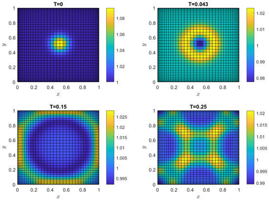
Figure 10. Water height $h(x,y,T)$ at various times T for Example 6.

To provide a consolidated overview of the algorithm’s performance across all test cases, the key findings are summarized in Table 3.

Table 3. Summary of key findings from numerical simulations.

Example	Problem Description	Dim.	Nodes	MAE (Height)	MAE (Velocity)
1	Lake at Rest	1D	100	$6.45\times {10}^{-12}$	$8.49\times {10}^{-13}$
2	Gaussian Pulse	1D	60	Reaches steady state *
3	Dam Break (Flat)	1D	200	$2.88\times {10}^{-3}$	$1.07\times {10}^{-2}$
4	Dam Break (Bump)	1D	100	Qualitative match †
5	Lake at Rest	2D	$30\times 30$	$2.50\times {10}^{-6}$	$7.77\times {10}^{-4}$
6	Gaussian Pulse	2D	$40\times 40$	Qualitative match ‡

* Reached steady state within a tolerance of ${10}^{-5}$. MAE is not applicable. ^† Gives the same behavior as methods in [8]. MAE is not applicable. ^‡ Behaves consistently with schemes in [13]. MAE is not applicable.

5. Conclusions

This study presents a robust numerical algorithm for solving one- and two-dimensional SWEs by applying the FIM-CPE. The method transforms the governing PDEs into integral equations, approximates spatial variables using Chebyshev polynomials, and utilizes forward differences for temporal discretization, with stability ensured by the Courant–Friedrichs–Lewy condition. The algorithm’s efficacy was rigorously validated through several benchmark cases.

For one-dimensional SWEs, the scheme demonstrated high precision in the lake at rest problem, with MAEs for water height and velocity below ${10}^{-12}$. In the dam-break scenario over a flat bottom, the FIM-CPE produced more accurate results compared to the traditional FDM and effectively captured shock propagation. Furthermore, the algorithm accurately simulated wave interactions over non-flat topographies and handled smooth solutions, as shown in the dam break over a bump and Gaussian pulse examples, respectively.

The method was extended to two-dimensional SWEs, where it successfully resolved wave interactions over complex topographies and accurately simulated phenomena such as a Gaussian-shaped peak. A key strength of the proposed scheme is its excellent mass conservation, with total volume deviations remaining under ${10}^{-5}$ across all simulations. While the proposed FIM-CPE scheme has proven to be a highly accurate and reliable simulation tool, we acknowledge its current limitations. The algorithm is presently formulated for wet-bed conditions and has been validated on small-scale problems, without considering frictional effects. Future work will focus on extending the algorithm’s capabilities. Key directions for development include incorporating wet–dry front tracking algorithms, including bed friction and Coriolis terms, and scaling the method for application to larger, real-world hydraulic and coastal engineering problems.

References

- De St Venant, B. Theorie du mouvement non-permanent des eaux avec application aux crues des rivers et a l’introduntion des Marees dans leur lit. Comptes Rendus Acad. Sci. 1871, 73, 148–154. [Google Scholar]
- Valiani, A.; Caleffi, V.; Zanni, A. Case study: Malpasset dam-break simulation using a two-dimensional finite volume method. J. Hydraul. Eng. 2002, 128, 460–472. [Google Scholar] [CrossRef]
- George, D.L. Finite Volume Methods and Adaptive Refinement for Tsunami Propagation and Inundation; University of Washington: Seattle, WA, USA, 2006. [Google Scholar]
- Mignot, E.; Paquier, A.; Haider, S. Modeling floods in a dense urban area using 2D shallow water equations. J. Hydrol. 2006, 327, 186–199. [Google Scholar] [CrossRef]
- Gunawan, H.P. Numerical Simulation of Shallow Water Equations and Related Models. Ph.D. Thesis, Université Paris-Est, Champs-sur-Marne, France, 2015. [Google Scholar]
- Sarkar, B.; De, S. Oblique wave diffraction by a bottom-standing thick barrier and a pair of partially immersed barriers. J. Offshore Mech. Arct. Eng. 2023, 145, 010905. [Google Scholar] [CrossRef]
- Mekchay, K.; Pongsanguansin, T.; Maleewong, M. Numerical Methods Based on Discontinuous Galerkin and Finite Volume Methods for Shallow Water Model and Applications. Ph.D. Thesis, Chulalongkorn University, Bangkok, Thailand, 2016. [Google Scholar]
- Hudson, J. Numerical Techniques for the Shallow Water Equations; University of Reading, Department of Mathematics: Reading, UK, 1999. [Google Scholar]
- Crowhurst, P.; Li, Z. Numerical solutions of one-dimensional shallow water equations. In Proceedings of the 2013 UKSim 15th International Conference on Computer Modelling and Simulation, Cambridge, UK, 10–12 April 2013; IEEE: Piscataway, NJ, USA, 2013; pp. 55–60. [Google Scholar]
- Peng, S.H. 1D and 2D Numerical Modeling for Solving Dam-Break Flow Problems Using Finite Volume Method. J. Appl. Math. 2012, 2012, 489269. [Google Scholar] [CrossRef]
- LeVeque, R.J. Balancing source terms and flux gradients in high-resolution Godunov methods: The quasi-steady wave-propagation algorithm. J. Comput. Phys. 1998, 146, 346–365. [Google Scholar] [CrossRef]
- San, O.; Kara, K. High-order accurate spectral difference method for shallow water equations. Int. J. Res. Rev. Appl. Sci. 2011, 6, 41–54. [Google Scholar]
- Lundgren, L. Efficient Numerical Methods for the Shallow Water Equations. Master’s Thesis, Uppsala University, Uppsala, Sweden, 2018. [Google Scholar]
- Boonklurb, R.; Duangpan, A.; Treeyaprasert, T. Modified finite integration method using Chebyshev polynomial for solving linear differential equations. J. Numer. Anal. Ind. Appl. Math. 2018, 12, 1–19. [Google Scholar]
- Boonklurb, R.; Duangpan, A. Finite Integration Method Using Chebyshev Expansion for Solving Nonlinear Poisson Equations on Irregular Domains. J. Numer. Anal. Ind. Appl. Math. 2020, 14, 7–24. [Google Scholar]
- Boonklurb, R.; Duangpan, A.; Saengsiritongchai, A. Finite integration method via Chebyshev polynomial expansion for solving 2-D linear time-dependent and linear space-fractional differential equations. Thai J. Math. 2020, 103–131. [Google Scholar]
- Duangpan, A.; Boonklurb, R. Numerical solution of time-fractional Benjamin-Bona-Mahony-Burgers equation via finite integration method by using Chebyshev expansion. Songklanakarin J. Sci. Technol. 2021, 43. [Google Scholar]
- Zhang, H.; Ding, F. On the Kronecker Products and Their Applications. J. Appl. Math. 2013, 2013, 296185. [Google Scholar] [CrossRef]
- Cyganek, B. Object Detection and Recognition in Digital Images: Theory and Practice; John Wiley & Sons: Hoboken, NJ, USA, 2013. [Google Scholar]
- Stoker, J.J. Water Waves: The Mathematical Theory with Applications; Courier Dover Publications: New York, NY, USA, 2019. [Google Scholar]
Disclaimer/Publisher’s Note: The statements, opinions and data contained in all publications are solely those of the individual author(s) and contributor(s) and not of MDPI and/or the editor(s). MDPI and/or the editor(s) disclaim responsibility for any injury to people or property resulting from any ideas, methods, instructions or products referred to in the content. |
© 2025 by the authors. Licensee MDPI, Basel, Switzerland. This article is an open access article distributed under the terms and conditions of the Creative Commons Attribution (CC BY) license (https://creativecommons.org/licenses/by/4.0/).