Spatiotemporal Dynamics of a Predator–Prey Model with Harvest and Disease in Prey

Abstract

In this paper, we propose a diffusion-type predator–prey interaction model with harvest and disease in prey, and conduct stability analysis and pattern formation analysis on the model. For the temporal model, the asymptotic stability of each equilibrium is analyzed using the linear stability method, and the conditions for Hopf bifurcation to occur near the positive equilibrium are investigated. The simulation results indicate that an increase in infection force might disrupt the stability of the model, while an increase in harvesting intensity would make the model stable. For the spatiotemporal model, a priori estimate for the positive steady state is obtained for the non-existence of the non-constant positive solution using maximum principle and Harnack inequality. The Leray–Schauder degree theory is used to study the sufficient conditions for the existence of non-constant positive steady states of the model, and pattern formation are achieved through numerical simulations. This indicates that the movement of prey and predators plays an important role in pattern formation, and different diffusions of these species may play essentially different effects.

1. Introduction

In mathematical biology, species interactions are crucial for sustaining ecosystem stability amid the fluctuations of natural environments. As essential tools for depicting such interactions, mathematical models have long captivated researchers. Among these, predator–prey relationships, a key driver of natural population dynamics, have been a central focus of ecologists and biologists in recent decades. Numerous researchers have studied interactions like predator–prey dynamics, mutualisms, and competitive mechanisms, striving to develop more biologically realistic models [1,2,3,4,5].

It is well-known that infectious diseases can impact ecological systems and regulate population density. Therefore, studying how epidemiological factors influence the dynamics of predator–prey interactions is vital for a better understanding of ecosystems. Anderson and May [6] pioneered the investigation into the invasion, persistence, and spread of infectious diseases by formulating an eco-epidemiological predator–prey model. In recent years, many researchers have proposed and analyzed epidemic and eco-epidemiological models [7,8,9,10,11,12,13,14,15]. For instance, Shaikh et al. [9] investigated the dynamics of an eco-epidemiological system with disease in competitive prey species. Xiao and Chen [10] analyzed persistence in a ratio-dependent prey-disease model, and demonstrated that predator infection might prevent prey extinction. Gao et al. [15] explored how transmission rates affect stability in bidirectional infection models.

Recently, Kar et al. [16] proposed and analyzed a predator–prey model with disease in prey population, which is formulated as follows:

$$\left\{\begin{array}{c}{\displaystyle \frac{\mathrm{d}S}{\mathrm{d}T}}=rS-{\displaystyle \frac{r{S}^2}{K}}-aSI-{\displaystyle \frac{bSP}{h+S}},\hfill \\ {\displaystyle \frac{\mathrm{d}I}{\mathrm{d}T}}=aSI-\sigma IP-\mu I,\hfill \\ {\displaystyle \frac{\mathrm{d}P}{\mathrm{d}T}}={\displaystyle \frac{lbSP}{h+S}}+ϵ\sigma IP-\delta P,\hfill \\ S\left(0\right)\ge 0,I\left(0\right)\ge 0,P\left(0\right)\ge 0,\hfill \end{array}\right.$$

(1)

where ${\displaystyle S\left(T\right),I\left(T\right),P\left(T\right)}$ represent the population densities of susceptible prey, infected prey and predator, respectively. ${\displaystyle r}$ and ${\displaystyle K}$ denote the intrinsic growth rate and environmental carrying capacity of susceptible prey population. ${\displaystyle a}$ is the infection force between infected and susceptible prey. ${\displaystyle b}$ stands for the maximum capturing rate of susceptible prey by predator, and ${\displaystyle h}$ is the half saturation constant. ${\displaystyle \sigma }$ is the maximum capturing rate of infected prey by predator. ${\displaystyle l}$ and ${\displaystyle ϵ}$ are the conversion factors. ${\displaystyle \mu }$ and ${\displaystyle \delta }$ are the natural death rates of infected prey and predators, respectively. All the above described parameters are assumed to be positive from a biological perspective. In [16], Kar and his collaborators performed theoretical and numerical analyses on the stability and bifurcation behavior of model (1) and derived necessary conditions for the optimal control of the prey using Pontrygin’s maximum principle.

However, most of the previous works on eco-epidemiological models did not consider the random diffusion which arises from a natural tendency to diffuse to areas of smaller population for species. In reality, prey and predator species, both infected and healthy ones, are inhomogeneously distributed in different ecological spaces at a given time and interact with other organisms present within their spatial domain. Therefore, this movement or diffusion process must be incorporated into temporal eco-epidemiological models that do not explicitly account for space. The resulting eco-epidemiological models are represented by reaction–diffusion equations. Recent studies have explored spatiotemporal dynamics of infected prey–predator systems [17,18,19,20]. Li et al. [17] examined an eco-epidemiological system with infected predators, identifying parameter ranges for Turing patterns. Chakraborty et al. [19] analyzed a diffusive model where predators feed on infected prey via a Type II response, with prey infection spreading horizontally, investigating spatiotemporal complexity. Melese and Feyissa [20] studied stability and bifurcation in a diffusive system with prey disease: predators use Beddington–DeAngelis responses for susceptible prey and Holling Type II for infected prey, though they did not explore non-constant positive steady states. Vitanov et al. [21] discussed a partial differential equations for description of the spatiotemporal dynamics of interacting populations and studied the waves caused by migration of the populations, they assumed that the migration is a diffusion process influenced by the changing values of the birth rates and coefficients of interaction among the populations.

Harvesting activities such as fishing and hunting have a profound impact on population dynamics. Hossain et al. [22] demonstrated that changes in capture intensity can affect the pattern structure of the model. Sun and Dai [23] found that adjusting the harvest can alleviate intraspecific competition pressure and stabilize the system under certain conditions. From the perspective of human needs, the exploitation of biological resources and population harvesting are common practices in fishery, forestry, and wildlife management. For the conservation of long-term benefits for humanity, there is considerable interest in using bioeconomic modeling to gain insights into the scientific management of renewable resources such as fisheries and forests [24,25]. Therefore, it is necessary to investigate the effects of species harvesting in relevant models. On the other hand, studies have confirmed that infected prey may exert negative impacts on predators. Parasites in infected prey may reduce the reproductive and survival rates of predators by impairing energy absorption [26,27], weakening the food conversion ability of predators [28,29]. These parasite-induced changes could inhibit predator growth.

Inspired by the above research, we establish the following reaction–diffusion equation based on model (1), incorporating factors including prey population harvesting, negative impact of infected prey on predators, density dependent death of predators, and spatial self diffusion of species:

$$\left\{\begin{array}{c}{\displaystyle \frac{\partial S(x,T)}{\partial T}}-D_S{\displaystyle \frac{{\partial }^{2}S}{\partial x^2}}=rS(1-{\displaystyle \frac{S}{K}})-aSI-{\displaystyle \frac{bSP}{h+S}}-Q_{1}ES,x\in (0,L),T>0,\hfill \\ {\displaystyle \frac{\partial I(x,T)}{\partial T}}-D_I{\displaystyle \frac{{\partial }^{2}I}{\partial x^2}}=aSI-\sigma IP-\mu I-Q_{2}EI,x\in (0,L),T>0,\hfill \\ {\displaystyle \frac{\partial P(x,T)}{\partial T}}-D_P{\displaystyle \frac{{\partial }^{2}P}{\partial x^2}}={\displaystyle \frac{lbSP}{h+S}}+(ϵ-{ϵ}_1)\sigma IP-\delta P-{\delta }_1{P}^2,x\in (0,L),T>0,\hfill \\ {\displaystyle \frac{\partial S(x,T)}{\partial x}}={\displaystyle \frac{\partial I(x,T)}{\partial x}}={\displaystyle \frac{\partial P(x,T)}{\partial x}}=0,x=0,L,T>0,\hfill \\ S(x,0)>0,I(x,0)>0,P(x,0)>0,x\in (0,L),\hfill \end{array}\right.$$

(2)

where ${\displaystyle S(x,T),I(x,T),P(x,T)}$ are, respectively, the population densities of susceptible prey, infected prey, and predator at time ${\displaystyle T}$ and position ${\displaystyle x}$, and the positive constants ${\displaystyle D_S,D_I,D_P}$ represent their diffusion coefficients. ${\displaystyle Q_1,Q_2}$ represent the harvest coefficients of susceptible and infected prey and ${\displaystyle E}$ is the harvesting effort. ${\displaystyle {ϵ}_1\sigma I(0\le {ϵ}_1<ϵ)}$ indicates the negative effect on the predator population due to the infection from the infected prey. ${\displaystyle {\delta }_1}$ denotes the density dependent mortality rate of the predator. The one-dimensional domain ${\displaystyle [0,L]\subset \mathit{R}}$ denotes the habitat of three species, and the operator ${\displaystyle {\partial }^2/\partial x^2}$ is used to describe the self-diffusion of species in ${\displaystyle [0,L]}$. The homogeneous Neumann boundary condition means that model (2) is self-contained and has no population flux across the boundary, and the initial values ${\displaystyle S(x,0),I(x,0),P(x,0)}$ are continuous functions. The meanings of other parameters are the same as those in model (1). Here we point out that the diffusion considered in this article is the self-diffusion of each species from high-density regions to low-density regions, which is different from [21,30]. In other words, in the established spatial model, we always ignore the impact of the migration of the other two populations.

Introducing the non-dimensional variables ${\displaystyle u=S/K,v=I/K,w=P/K,t=rT}$ and scaling the parameters, the model (2) is transformed to the following non-dimensional model:

$$\left\{\begin{array}{c}{\displaystyle \frac{\partial u(x,t)}{\partial t}}-D_1{\displaystyle \frac{{\partial }^{2}u}{\partial x^2}}=u(1-u)-\alpha uv-{\displaystyle \frac{\beta uw}{c+u}}-q_{1}u,x\in (0,L),t>0,\hfill \\ {\displaystyle \frac{\partial v(x,t)}{\partial t}}-D_2{\displaystyle \frac{{\partial }^{2}v}{\partial x^2}}=\alpha uv-\gamma vw-d_{1}v-q_{2}v,x\in (0,L),t>0,\hfill \\ {\displaystyle \frac{\partial w(x,t)}{\partial t}}-D_3{\displaystyle \frac{{\partial }^{2}w}{\partial x^2}}=l\left({\displaystyle \frac{\beta uw}{c+u}}+(m-n)\gamma vw-d_{2}w-d_3{w}^2\right),x\in (0,L),t>0,\hfill \\ {\displaystyle \frac{\partial u(x,t)}{\partial x}}={\displaystyle \frac{\partial v(x,t)}{\partial x}}={\displaystyle \frac{\partial w(x,t)}{\partial x}}=0,x=0,L,t>0,\hfill \\ u(x,0)>0,v(x,0)>0,w(x,0)>0,x\in (0,L),\hfill \end{array}\right.$$

(3)

where ${\displaystyle \alpha =\frac{aK}{r},\beta =\frac{b}{r},c=\frac{h}{K},\gamma =\frac{\sigma K}{r},d_1=\frac{\mu }{r},m=\frac{ϵ}{l},n=\frac{{ϵ}_1}{l},d_2=\frac{\delta }{lr},d_3=\frac{{\delta }_{1}K}{lr},q_1=\frac{Q_{1}E}{r},q_2=\frac{Q_{2}E}{r}}$, ${\displaystyle D_1=\frac{D_S}{r},D_2=\frac{D_I}{r},D_3=\frac{D_P}{r}.}$ The main purpose of this paper is to reveal the synergistic effects of disease transmission between prey and harvesting on the corresponding time model dynamics, and to analyze the impact of different species diffusion rates on the existence of non-homogeneous steady-state solutions in spatiotemporal models. Our research results will indicate that excessive capture of susceptible prey may lead to disease and predator extinction in the time model, while disease transmission and human capture have opposite effects on model stability. When all the diffusion rates of the species are high, the system will not exhibit non-homogeneous steady states. Under certain conditions, only when the diffusion rate of one of the three species is higher, the system will produce spatially non-homogeneous steady states.

The remainder of this paper is structured as follows: In Section 2, the dynamics of the temporal model are investigated through local stability analysis, with equilibrium existence, stability, and Hopf bifurcation conditions addressed. In Section 3, a prior estimate of the positive steady states for the spatiotemporal model is established, and Leray–Schauder degree theory and energy methods are employed to determine existence and non-existence criteria for non-constant positive steady states in model (3). In Section 4, a concise summary and discussion of the findings are presented.

2. Dynamics of the Temporal Model

In this section, we first study the dynamics of the temporal model corresponding to model (3), that is,

$$\left\{\begin{array}{c}{\displaystyle \frac{\mathrm{d}u\left(t\right)}{\mathrm{d}t}}=u(1-u)-\alpha uv-{\displaystyle \frac{\beta uw}{c+u}}-q_{1}u,t>0,\hfill \\ {\displaystyle \frac{\mathrm{d}v\left(t\right)}{\mathrm{d}t}}=\alpha uv-\gamma vw-d_{1}v-q_{2}v,t>0,\hfill \\ {\displaystyle \frac{\mathrm{d}w\left(t\right)}{\mathrm{d}t}}=lw\left({\displaystyle \frac{\beta u}{c+u}}+(m-n)\gamma v-d_2-d_{3}w\right),t>0,\hfill \\ u\left(0\right)>0,v\left(0\right)>0,w\left(0\right)>0.\hfill \end{array}\right.$$

(4)

2.1. Boundedness and Equilibria

Theorem 1.

All solutions of model (4) with initial value ${\displaystyle \left(u\right(0),v(0),w(0\left)\right)}$ in ${\displaystyle {\mathit{R}}_{+}^3}$ are non-negetive and uniformly bounded.

Proof. 

Let ${\displaystyle \left(u\right(t),v(t),w(t\left)\right)}$ be any solution to the temporal model (4) starting from ${\displaystyle {\mathit{R}}_{+}^3}$. Note that

$$\begin{array}{cc}\hfill u\left(t\right)& =u\left(0\right)exp{\int }_0^t\left\{1-q_1-u\left(\tau \right)-\alpha v\left(\tau \right)-{\displaystyle \frac{\beta w\left(\tau \right)}{c+u\left(\tau \right)}}-q_1\right\}d\tau ,\hfill \\ \hfill v\left(t\right)& =v\left(0\right)exp{\int }_0^t\left\{\alpha u\left(\tau \right)-\gamma w\left(\tau \right)-d_1-q_2\right\}d\tau ,\hfill \\ \hfill w\left(t\right)& =w\left(0\right)exp{\int }_0^t\left\{{\displaystyle \frac{\beta lu\left(\tau \right)}{c+u\left(\tau \right)}}+l(m-n)\gamma v\left(\tau \right)-l{d}_2-l{d}_{3}w\left(\tau \right)\right\}d\tau .\hfill \end{array}$$

Therefore the solution ${\displaystyle \left(u\right(t),v(t),w(t\left)\right)}$ is non-negative. Next, we prove that the solution ${\displaystyle \left(u\right(t),v(t),w(t\left)\right)}$ has positive upper bounds.

First, for the case ${\displaystyle m-n<1}$, introduce the auxiliary variable ${\displaystyle X=u+v+\frac{w}{l}}$. Taking the derivative of ${\displaystyle X}$ with respect to ${\displaystyle t}$ yields

$$\begin{array}{cc}\hfill {\displaystyle \frac{\mathrm{d}X}{\mathrm{d}t}}& =u(1-u)-(1-(m-n))\gamma vw-q_{1}u-(d_1+q_2)v-d_{2}w-d_3{w}^2\hfill \\ \hfill & \le u(1-u)-q_{1}u-(d_1+q_2)v-d_{2}w.\hfill \end{array}$$

(5)

Let ${\displaystyle L=min\{q_1,d_1+q_2,l{d}_2\}>0}$. From (5), it follows that ${\displaystyle \frac{\mathrm{d}X}{\mathrm{d}t}+LX\le u(1-u)\le \frac{1}{4}.}$ Applying the theorem of differential inequality theorem, we obtain

$$X\left(t\right)\le {\displaystyle \frac{1}{4L}}(1-e^{-Lt})+X\left(0\right)e^{-Lt}.$$

Hence, any solution of (4) initiated in ${\displaystyle {\mathit{R}}_{+}^3}$ is eventually confined in the region

$${\Omega }_1=\left\{(u,v,w)\in {\mathit{R}}_{+}^3|0\le u+v+{\displaystyle \frac{w}{l}}\le {\displaystyle \frac{1}{4L}}+ϵ\right\}$$

for any ${\displaystyle ϵ>0}$ and for ${\displaystyle t\to \infty }$.

For ${\displaystyle m-n\ge 1}$, define ${\displaystyle X=u+v+\frac{w}{l(m-n)}}$. Differentiating ${\displaystyle X}$ with respect to ${\displaystyle t}$ gives

$$\begin{array}{cc}\hfill {\displaystyle \frac{\mathrm{d}X}{\mathrm{d}t}}& =u(1-u)-\left(1-{\displaystyle \frac{1}{m-n}}\right){\displaystyle \frac{\beta uw}{c+u}}-q_{1}u-(d_1+q_2)v-{\displaystyle \frac{d_2}{m-n}}w-{\displaystyle \frac{d_3}{m-n}}{w}^2\hfill \\ \hfill & \le u(1-u)-q_{1}u-(d_1+q_2)v-{\displaystyle \frac{d_2}{m-n}}w.\hfill \end{array}$$

Let ${\displaystyle L=min\{q_1,d_1+q_2,l{d}_2\}>0}$. It follows the above inequality that ${\displaystyle \frac{\mathrm{d}X}{\mathrm{d}t}+LX\le u(1-u)\le \frac{1}{4}.}$ Applying the theorem of differential inequality again, we obtain ${\displaystyle X\left(t\right)\le \frac{1}{4L}(1-e^{-Lt})+X\left(t\right)e^{-Lt}.}$ Hence, all solutions of (4) with initial values in ${\displaystyle {\mathit{R}}_{+}^3}$ are confined in the region

$${\Omega }_2=\{(u,v,w)\in {\mathit{R}}_{+}^3|0\le u+v+{\displaystyle \frac{w}{l(m-n)}}\le {\displaystyle \frac{1}{4L}}+ϵ\}$$

for any ${\displaystyle ϵ>0}$ and for ${\displaystyle t\to \infty }$. The theorem is thus proved. ${\displaystyle \square }$

Next, we focus to discuss the equilibria of model (4). It is easy to verify that model (4) has five possible equilibrium states, namely the following:

(i)

The trivial equilibrium ${\displaystyle E_0(0,0,0)}$.

(ii)

The boundary equilibrium ${\displaystyle E_1(1-q_1,0,0)}$, which is feasible since ${\displaystyle q_1<1}$ in a biological sense.

(iii)

The infection prey free equilibrium ${\displaystyle E_2(u_2,0,w_2)}$; where ${\displaystyle w_2=\frac{1}{\beta }(1-u_2-q_1)(c+u_2)}$ and ${\displaystyle u_2}$ is a positive root of cubic equation ${\displaystyle d_3(1-q_1-u){(c+u)}^2+d_2\beta (c+u)={\beta }^{2}u}$, the equilibrium is feasible for ${\displaystyle 0<\frac{d_{2}c}{\beta -d_2}<u_2<1-q_1}$.

(iv)

The predator free equilibrium ${\displaystyle E_3(u_3,v_3,0)}$; where ${\displaystyle u_3=\frac{d_1+q_2}{\alpha },v_3=\frac{\alpha (1-q_1)-(d_1+q_2)}{{\alpha }^2}}$, the equilibrium is feasible for ${\displaystyle 1-q_1>\frac{d_1+q_2}{\alpha }}$.

(v)

The coexistence equilibrium ${\displaystyle E^{\ast }(u^{\ast },v^{\ast },w^{\ast })}$, where ${\displaystyle v^{\ast }=\frac{1}{(m-n)\gamma }\left(d_2+d_3{w}^{\ast }-\frac{\beta u^{\ast }}{c+u^{\ast }}\right)}$, ${\displaystyle w^{\ast }=\frac{\alpha u^{\ast }-d_1-q_2}{\gamma }}$ and ${\displaystyle u^{\ast }}$ is a positive root of equation

$$k_1{u}^2+k_{2}u+k_3=0,$$

(6)

with

$$\begin{array}{cc}\hfill k_1& =(m-n){\gamma }^2+{\alpha }^2{d}_3>0,\hfill \\ \hfill k_2& =(m-n)\gamma (\alpha \beta +\gamma c+\gamma q_1-\gamma )+\alpha \gamma (d_2-\beta )+\alpha d_3(\alpha c-d_1-q_2),\hfill \\ \hfill k_3& =\alpha c(\gamma d_2-d_1{d}_3-q_2{d}_3)-(m-n)\gamma (\beta d_1+\beta q_2+\gamma c-\gamma c{q}_1).\hfill \end{array}$$

For the existence of ${\displaystyle v^{\ast }}$ and ${\displaystyle w^{\ast }}$, it is necessary that

$${\displaystyle \frac{d_1+q_2}{\alpha }}<u^{\ast }<{\displaystyle \frac{(d_2+d_3{w}^{\ast })c}{\beta -d_2-d_3{w}^{\ast }}}.$$

(7)

For the existence of ${\displaystyle u^{\ast }}$, we consider the following two cases.

Case 1: If ${\displaystyle k_3<0}$, then Equation (6) has a unique positive root given by

$$u^{\ast }={\displaystyle \frac{-k_2+\sqrt{k_2^2-4k_1{k}_3}}{2k_1}}.$$

Case 2: If ${\displaystyle k_3>0,k_2<0}$ and ${\displaystyle k_2^2>4k_1{k}_3}$, then (6) has two different positive roots.

Remark 1.

The above two cases also correspond to the number of positive equilibria of the temporal model (4). For the condition of the existence of unique positive equilibrium, i.e., ${\displaystyle k_3<0}$, we can obtain the range of ${\displaystyle \alpha }$ given by ${\displaystyle 0\le \alpha <{\alpha }_{max}}$, where

$${\alpha }_{max}={\displaystyle \frac{(m-n)\gamma (\beta d_1+\beta q_2+\gamma c-\gamma c{q}_1)}{c(\gamma d_2-d_1{d}_3-q_2{d}_3)}}.$$

(8)

From (8), we can see that the maximum value of the infection rate ${\displaystyle {\alpha }_{max}}$ of the susceptible prey population is inversely proportional to the mortality rate of the predator population ${\displaystyle q_1}$. That is to say, if the harvest intensity of the susceptible prey decreases, the maximum value of the infection rate of the susceptible prey population will increase, and vice versa.

2.2. Local Asymptotic Stability and Hopf Bifurcation

In this section, we conduct a linear stability analysis on the equilibria obtained in the previous section to determine their local stability. Next, we will omit the specific derivation process and directly present the local stability results for the equilibria ${\displaystyle E_0,E_1,E_2}$, and ${\displaystyle E_3}$. The details are as follows:

(i)

${\displaystyle E_0}$ is always unstable.

(ii)

${\displaystyle E_1}$ is locally stable when ${\displaystyle 1-q_1<min\{\frac{d_1+q_2}{\alpha },\frac{c{d}_2}{\beta -d_2}\}}$, unstable when ${\displaystyle 1-q_1>min\{\frac{d_1+q_2}{\alpha },\frac{c{d}_2}{\beta -d_2}\}}$.

(iii)

${\displaystyle E_2}$ is stable when ${\displaystyle \frac{\alpha u_2-d_1-q_2}{\gamma }<w_2<min\{\frac{u_2{(c+u_2)}^2}{\beta u_2-d_{3}l{(c+u_2)}^2},\frac{d_3{(c+u_2)}^3+{\beta }^{2}c}{d_3\beta (c+u_2)}\},}$ unstable when ${\displaystyle w_2<\frac{\alpha u_2-d_1-q_2}{\gamma }}$ or ${\displaystyle w_2>min\{\frac{u_2{(c+u_2)}^2}{\beta u_2-d_{3}l{(c+u_2)}^2},\frac{d_3{(c+u_2)}^3+{\beta }^{2}c}{d_3\beta (c+u_2)}\}.}$

(iv)

${\displaystyle E_3}$ is locally stable when ${\displaystyle v_3<\frac{d_{2}c+(d_2-\beta )u_3}{\gamma (m-n)(c+u_3)}}$, unstable when ${\displaystyle v_3>\frac{d_{2}c+(d_2-\beta )u_3}{\gamma (m-n)(c+u_3)}}$.

Remark 2.

Through simple calculations, we can find that the local asymptotic stability of ${\displaystyle E_1}$ means that the equilibria ${\displaystyle E_2,E_3}$, and ${\displaystyle E^{\ast }}$ do not exist. That is to say, an increase in the harvest intensities ${\displaystyle q_1,q_2}$ of the prey population may lead to the extinction of diseased prey and predators, and only susceptible prey will survive. This is detrimental to the survival of the predators.

Now we begin to derive the local asymptotic stability condition of the positive equilibrium ${\displaystyle E^{\ast }}$. Linearizing model (4) around the positive equilibrium ${\displaystyle E^{\ast }}$, we can obtain the Jacobin matrix ${\displaystyle J_{E^{\ast }}={\left(a_{ij}\right)}_{3\times 3}}$ and the following characteristic equation

$${\lambda }^3+M_2{\lambda }^2+M_1\lambda +M_0=0,$$

(9)

where

$$\begin{array}{cc}\hfill M_2& =-a_{11}-a_{33},M_1=a_{11}{a}_{33}-a_{12}{a}_{21}-a_{23}{a}_{32}-a_{13}{a}_{31},\hfill \\ \hfill M_0& =a_{11}{a}_{23}{a}_{32}+a_{12}{a}_{21}{a}_{33}-a_{12}{a}_{23}{a}_{31}-a_{13}{a}_{21}{a}_{32},\hfill \end{array}$$

(10)

with

$$\begin{array}{cc}\hfill a_{11}& =-u^{\ast }+{\displaystyle \frac{\beta u^{\ast }{w}^{\ast }}{{(c+u^{\ast })}^2}},a_{12}=-\alpha u^{\ast },a_{13}=-{\displaystyle \frac{\beta u^{\ast }}{c+u^{\ast }}},a_{21}=\alpha v^{\ast },\hfill \\ \hfill a_{23}& =-\gamma v^{\ast },a_{31}={\displaystyle \frac{l\beta c{w}^{\ast }}{{(c+u^{\ast })}^2}},a_{32}=l\gamma (m-n)w^{\ast },a_{33}=-d_{3}l{w}^{\ast }.\hfill \end{array}$$

(11)

According to Routh–Hurwitz criteria, all the roots of characteristic Equation (9) have negative real parts if and only if

$$M_2>0,M_0>0,M_1{M}_2>M_0.$$

(12)

Theorem 2.

The positive equilibrium ${\displaystyle E^{\ast }}$ of model (4) is locally stable if and only if the conditions (12) hold.

It can be directly calculated that conditions (12) hold if ${\displaystyle \frac{\beta w^{\ast }}{{(c+u^{\ast })}^2}<1}$. Therefore, we can obtain the following sufficient condition for the stability of the positive equilibrium ${\displaystyle E^{\ast }}$.

Corollary 1.

If ${\displaystyle \frac{\beta w^{\ast }}{{(c+u^{\ast })}^2}<1}$, then the positive equilibrium ${\displaystyle E^{\ast }}$ of model (4) is locally asymptotically stable.

Taking the infection force ${\displaystyle \alpha }$ as the bifurcation parameter, it is easy to obtain the following Hopf bifurcation results near the positive equilibrium of model (4).

Lemma 1.

Let ${\displaystyle E^{\ast }}$ be a positive equilibrium of model (4) and ${\displaystyle M_i(i=0,1,2)}$ be defined in (10). Assuming that there exists a critical value ${\displaystyle {\alpha }_h}$ such that (i) ${\displaystyle M_2\left({\alpha }_h\right)M_1\left({\alpha }_h\right)=M_0\left({\alpha }_h\right),M_i\left({\alpha }_h\right)>0(i=0,1,2)}$ and (ii) ${\displaystyle {\dot{M}}_0\left({\alpha }_h\right)\ne 0}$ are satisfied. Then model (4) will undergo a Hopf bifurcation at equilibrium ${\displaystyle E^{\ast }}$ when ${\displaystyle \alpha }$ passes through ${\displaystyle {\alpha }_h}$.

Proof. 

Let ${\displaystyle {\lambda }_1,{\lambda }_2,{\lambda }_3}$ be the eigenvalues to Equation (9), then ${\displaystyle M_2=-({\lambda }_1+{\lambda }_2+{\lambda }_3),M_1={\lambda }_1{\lambda }_2+{\lambda }_2{\lambda }_3+{\lambda }_1{\lambda }_3,M_0=-{\lambda }_1{\lambda }_2{\lambda }_3}$. Hopf bifurcation occurs when the real parts of two eigenvalues passes through zero while the other one eigenvalue still has negative real parts and the the transversality condition is satisfied, that is, there exists a critical value ${\displaystyle {\alpha }_h}$ of ${\displaystyle \alpha }$ such that (i) ${\displaystyle M_2\left({\alpha }_h\right)M_1\left({\alpha }_h\right)=M_0\left({\alpha }_h\right)}$ with ${\displaystyle M_0\left({\alpha }_h\right)>0,M_1\left({\alpha }_h\right)>0,M_2\left({\alpha }_h\right)>0}$ and the transversality condition (ii) ${\displaystyle {(\mathrm{d}/\mathrm{d}\alpha )\left(\mathrm{Re}\left(\lambda \left(\alpha \right)\right)\right)|}_{\alpha ={\alpha }_h}\ne 0}$ are satisfied.

When ${\displaystyle \alpha ={\alpha }_h}$, the characteristic equation (9) is given by

$$({\lambda }^2+M_1)(\lambda +M_2)=0$$

with roots ${\displaystyle {\lambda }_{1,2}=\pm i\sqrt{M_1}}$ and ${\displaystyle {\lambda }_3=-M_2}$. For ${\displaystyle \alpha }$ in a small neighborhood of ${\displaystyle {\alpha }_h}$, the eigenvalues have the forms ${\displaystyle {\lambda }_1\left(\alpha \right)=q_1\left(\alpha \right)+i{q}_2\left(\alpha \right),{\lambda }_2\left(\alpha \right)=q_1\left(\alpha \right)-i{q}_2\left(\alpha \right)}$ and ${\displaystyle {\lambda }_3\left(\alpha \right)=-q_3\left(\alpha \right)}$, where ${\displaystyle q_1\left(\alpha \right),q_2\left(\alpha \right)}$ and ${\displaystyle q_3\left(\alpha \right)}$ are real.

Now, we verify the transversality condition ${\displaystyle \frac{\mathrm{d}}{\mathrm{d}\alpha }\left(\mathrm{Re}\left({\lambda }_1\left(\alpha \right)\right)\right){|}_{\alpha ={\alpha }_h}\ne 0}$. By substituting ${\displaystyle \lambda =q_1\left(\alpha \right)+i{q}_2\left(\alpha \right)}$ into (9) and taking the derivative of ${\displaystyle \alpha }$, we obtain

$$\Phi \left(\alpha \right){\dot{q}}_1\left(\alpha \right)-\Psi \left(\alpha \right){\dot{q}}_2\left(\alpha \right)+{\Gamma }_1\left(\alpha \right)=0,$$

$$\Psi \left(\alpha \right){\dot{q}}_1\left(\alpha \right)+\Phi \left(\alpha \right){\dot{q}}_2\left(\alpha \right)+{\Gamma }_2\left(\alpha \right)=0,$$

where

$$\begin{array}{cc}\hfill \Phi \left(\alpha \right)& =3{\left(q_1\left(\alpha \right)\right)}^2-3{\left(q_2\left(\alpha \right)\right)}^2+2M_2\left(\alpha \right)q_1\left(\alpha \right)+M_1\left(\alpha \right),\hfill \\ \hfill \Psi \left(\alpha \right)& =6q_1\left(\alpha \right)q_2\left(\alpha \right)+2M_2\left(\alpha \right)q_2\left(\alpha \right),\hfill \\ \hfill {\Gamma }_1\left(\alpha \right)& ={\left(q_1\left(\alpha \right)\right)}^2{\dot{M}}_2\left(\alpha \right)-{\left(q_2\left(\alpha \right)\right)}^2{\dot{M}}_2\left(\alpha \right)+q_1\left(\alpha \right){\dot{M}}_1\left(\alpha \right)+{\dot{M}}_0\left(\alpha \right),\hfill \\ \hfill {\Gamma }_2\left(\alpha \right)& =2q_1\left(\alpha \right)q_2\left(\alpha \right){\dot{M}}_2\left(\alpha \right)+q_2\left(\alpha \right){\dot{M}}_1\left(\alpha \right).\hfill \end{array}$$

Now

$${\displaystyle \frac{\mathrm{d}}{\mathrm{d}\alpha }}\left(\mathrm{Re}\left({\lambda }_1\left(\alpha \right)\right)\right){|}_{\alpha ={\alpha }_h}={\displaystyle \frac{\mathrm{d}{q}_1\left(\alpha \right)}{\mathrm{d}\alpha }}{|}_{\alpha ={\alpha }_h}=-{\displaystyle \frac{\Phi {\Gamma }_1+\Psi {\Gamma }_2}{{\Phi }^2+{\Psi }^2}}{|}_{\alpha ={\alpha }_h}=-{\displaystyle \frac{M_1\left({\alpha }_h\right){\dot{M}}_0\left({\alpha }_h\right)}{{\Phi }^2\left({\alpha }_h\right)+{\Psi }^2\left({\alpha }_h\right)}}\ne 0$$

due to ${\displaystyle {\dot{M}}_0\left({\alpha }_h\right)M_1\left({\alpha }_h\right)\ne 0}$, and ${\displaystyle q_3\left({\alpha }_h\right)=-M_2\left({\alpha }_h\right)\ne 0}$, hence the transversality condition is satisfied. This completes the proof. ${\displaystyle \square }$

We conduct some numerical simulations to investigate the characteristics of the model (4) when some key parameters change. By changing the parameter ${\displaystyle q}$ while keeping other parameters constant (assuming ${\displaystyle q_1=q_2=q}$), the result is shown in Figure 1. From Figure 1a, it can be observed that an increase in harvest intensity leads to a decrease in total prey density and an increase in predator density. Figure 1b shows that the density of susceptible prey also increases with an increase in harvest intensity. In addition, we also simulated the effect of parameter ${\displaystyle n}$ (reflecting the negative impact of infected prey on predators) on the model solution (see Figure 2). Figure 2a shows that the total density of prey increases with an increase in ${\displaystyle n}$, while the density of predators decreases accordingly, and Figure 2b shows that the total density of susceptible prey decreases with an increase in ${\displaystyle n}$.

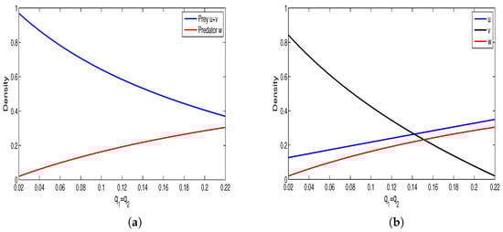
Figure 1. (a) Relationships between ${\displaystyle u+v,w}$ and the harvest coefficient ${\displaystyle q_1=q_2}$. (b) Relationships between ${\displaystyle u,v,w}$ and the harvest coefficient ${\displaystyle q_1=q_2}$. Here α = 0.95, β = 0.9, c = 0.33, γ = 0.04, d₁ = 0.1, d₂ = 0.25, d₃ = 0.7, m = 0.9, n = 0.5, l = 0.5.

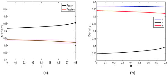
Figure 2. (a) Relationships between ${\displaystyle u,v,w}$ and the negative effect of infected prey ${\displaystyle n}$. (b) Relationships between ${\displaystyle u+v}$, ${\displaystyle w}$ and the negative effect of infected prey ${\displaystyle n}$. Here α = 0.95, β = 0.9, c = 0.33,γ = 0.04, d₁ = 0.1, d₂ = 0.25, d₃ = 0.7, q₁ = 0.15, q₂ = 0.15, m = 0.9, l = 0.5.

With the help of the drawing tool MATLAB R2021a, we use the continuation method to obtain the maximum and minimum values of the solution curves within a certain range as the bifurcation parameter ${\displaystyle \alpha }$ or ${\displaystyle q_1=q_2=q}$ continuously changes, and obtain the Hopf bifurcation curves. The results are shown in Figure 3 and Figure 4. By changing the value of ${\displaystyle \alpha }$ (reflecting the infection force), we observe that the coexistence equilibrium ${\displaystyle E^{\ast }}$ loses its stability and undergoes Hopf bifurcation when ${\displaystyle \alpha >{\alpha }_h=9.35}$, and a stable limit cycle appears when ${\displaystyle \alpha }$ is greater than the critical value ${\displaystyle {\alpha }_h}$. as shown in Figure 3a. Figure 3b shows the solution trajectory of model (4) starting from ${\displaystyle (0.10,0.15,0.06)}$ when ${\displaystyle \alpha =9.5>{\alpha }_h}$. Figure 3c and Figure 3d are the time series diagrams of model (4) when ${\displaystyle \alpha =8.8}$ and ${\displaystyle \alpha =9.5}$, respectively. By changing the value of ${\displaystyle q}$, we observe that the coexistence equilibrium ${\displaystyle E^{\ast }}$ loses its stability and undergoes Hopf bifurcation when parameter ${\displaystyle q}$ decreases through ${\displaystyle q_h=0.12}$, and a stable limit cycle appears when ${\displaystyle q}$ is lower than ${\displaystyle q_h}$ as ${\displaystyle q}$ decreases, as shown in Figure 4a. Figure 4b shows that a stable limit cycle occurs when ${\displaystyle q=0.093}$. Figure 4c and Figure 4d are the time series diagrams of model (4) when ${\displaystyle q=0.093}$ and ${\displaystyle q=0.14}$, respectively.

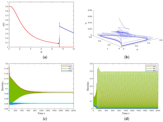
Figure 3. (a) Bifurcation diagram of model (4) with varying infection force ${\displaystyle \alpha }$. (b) The phase diagram of the model (4) when ${\displaystyle \alpha =9.5>{\alpha }_h}$. (c) Time series diagram of model (4) when ${\displaystyle \alpha =8.8}$. (d) Time series diagram of model (4) when ${\displaystyle \alpha =9.5}$. Other parameter values are β = 0.17, c = 0.004, γ = 10, d₁ = 0.25, d₂ = 0.2, d₃ = 0.7, m = 0.6, n = 0.3, q₁ = 0.1, q₂ = 0.1, l = 0.5.

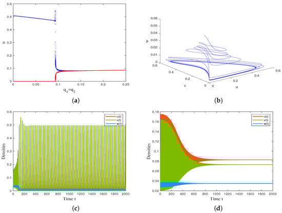
Figure 4. (a) Bifurcation diagram of model (4) with varying infection force ${\displaystyle q}$. (b) The phase diagram of the model (4) when ${\displaystyle q=0.093<q_h}$. (c) Time series diagram of model (4) when ${\displaystyle q=0.093}$. (d) Time series diagram of model (4) when ${\displaystyle q=0.14}$. Other parameter values are α = 9.3, β = 0.17, c = 0.004, γ = 10, d₁ = 0.25, d₂ = 0.2, d₃ = 5.2, m = 0.6, n = 0.3, l = 0.5.

Remark 3.

Figure 1 shows that increased prey harvesting decreases diseased prey density while increasing susceptible prey and predator densities. Biologically, intensified harvesting rapidly depletes diseased prey, reducing infection risk for susceptible prey and allowing their population to grow. This increase in high-quality food (susceptible prey) subsequently boosts the predator population. Conversely, Figure 2 shows the opposite trend: as the negative effects of diseased prey on predators increase, predator and susceptible prey densities decline while diseased prey density rises. Biologically, stronger negative effects reduce predator numbers. This reduced predation pressure allows diseased prey to increase, which likely drives the decline in susceptible prey through heightened infection.

3. Dynamics of the Spatiotemporal Model (3)

In the previous section, we analyzed the dynamics of the temporal model (4) and indicated that the model presents rich dynamic behaviors. In this section, we focus on analyzing the influence of the spatial diffusion on the dynamical behavior of model (3), including the existence and non-existence of spatial non-constant positive steady states.

3.1. A Prior Estimates of Positive Solutions

In order to discuss the existence of non-constant positive solutions, it is necessary to provide the upper and lower bounds of positive solutions to model (3) in the form of positive constants. For convenience, let us denote the constants ${\displaystyle \alpha ,\beta ,c,\gamma ,q_1,q_2,d_1,d_2,d_3,l,m,n}$ collectively by ${\displaystyle \Lambda }$. To investigate the non-existence and existence of the non-constant positive steady states of model (3), we consider the following elliptic system:

$$\left\{\begin{array}{c}-D_1{u}_{xx}=u(1-u)-\alpha uv-{\displaystyle \frac{\beta uw}{c+u}}-q_{1}u\equiv H_1(u,v,w),\mathrm{in}(0,L),\hfill \\ -D_2{v}_{xx}=\alpha uv-\gamma vw-d_{1}v-q_{2}v\equiv H_2(u,v,w),\mathrm{in}(0,L),\hfill \\ -D_3{w}_{xx}=l\left({\displaystyle \frac{\beta uw}{c+u}}+(m-n)\gamma vw-d_{2}w-d_3{w}^2\right)\equiv H_3(u,v,w),\mathrm{in}(0,L),\hfill \\ u_x\left(0\right)=u_x\left(L\right)=0,v_x\left(0\right)=v_x\left(L\right)=0,w_x\left(0\right)=w_x\left(L\right)=0,\hfill \end{array}\right.$$

(13)

where ${\displaystyle u_{xx},v_{xx},w_{xx}}$ represent the second derivatives with respect to ${\displaystyle x}$, and ${\displaystyle u_x,v_x,w_x}$ represent the first derivatives with respect to ${\displaystyle x}$.

For this purpose, we need to make use of the following maximum principle and Harnack inequality.

Proposition 1.

(maximum principle) [31] Let ${\displaystyle g\in C(\Omega \times \mathit{R})}$ and ${\displaystyle b_i\in C\left(\overline{\Omega }\right),i=1,2,\cdots ,N.}$

(i)

If ${\displaystyle \omega \in C^2(\Omega )\cap C^1\left(\overline{\Omega }\right)}$ satisfies ${\displaystyle \Delta \omega \left(x\right)+{\Sigma }_i^N{b}_i\left(x\right){\omega }_{x_i}+g(x,\omega \left(x\right))\ge 0}$ in ${\displaystyle \Omega ,\frac{\partial \omega }{\partial \nu }\le 0}$ on ${\displaystyle \partial \Omega }$ and ${\displaystyle \omega \left(x_0\right)=\underset{\overline{\Omega }}{max}\omega \left(x\right)}$, then ${\displaystyle g(x_0,\omega \left(x_0\right))\ge 0}$.

(ii)

If ${\displaystyle \omega \in C^2(\Omega )\cap C^1\left(\overline{\Omega }\right)}$ satisfies ${\displaystyle \Delta \omega \left(x\right)+{\Sigma }_i^N{b}_i\left(x\right){\omega }_{x_i}+g(x,\omega \left(x\right))\le 0}$ in ${\displaystyle \Omega ,\frac{\partial \omega }{\partial \nu }\ge 0}$ on ${\displaystyle \partial \Omega }$ and ${\displaystyle \omega \left(x_0\right)=\underset{\overline{\Omega }}{max}\omega \left(x\right)}$, then ${\displaystyle g(x_0,\omega \left(x_0\right))\le 0}$.

Proposition 2.

(Harnack inequality) [32] Let ${\displaystyle \omega \in C^2(\Omega )\cap C^1\left(\overline{\Omega }\right)}$ be a positive classical solution to ${\displaystyle \Delta \omega \left(x\right)+c\left(x\right)\omega \left(x\right)=0,c\left(x\right)\in C\left(\overline{\Omega }\right)}$, satisfying the zero flux boundary condition. Then there exists a positive constant ${\displaystyle C_{\ast }=C_{\ast }{(\Lambda ,\Omega ,\parallel c\parallel }_{\infty })}$ such that

$$\underset{\overline{\Omega }}{max}\omega \left(x\right)\le C_{\ast }\underset{\overline{\Omega }}{min}\omega \left(x\right).$$

Theorem 3.

Let ${\displaystyle \left(u\right(x),v(x),w(x\left)\right)}$ be a positive solution of (13). Suppose that

$$\alpha (a-q_1)>max\{{\displaystyle \frac{\beta +\gamma c}{c}}{N}_3+d_1+q_2,{\alpha }^2{N}_2+\gamma N_3+d_1+q_2\},$$

(14)

then there exists a positive constant ${\displaystyle C=C(\Lambda )}$ such that

$$C^{-1}<u\left(x\right)<C,C^{-1}<v\left(x\right)<C,C^{-1}<w\left(x\right)<C,$$

where ${\displaystyle N_1}$ and ${\displaystyle N_2}$ are defined in (15) and (16).

Proof. 

Suppose ${\displaystyle \left(u\right(x),v(x),w(x\left)\right)}$ is a positive solution to elliptic system (13). Let ${\displaystyle x_0\in [0,L]}$ be a point that satisfies ${\displaystyle u\left(x_0\right)=\underset{[0,L]}{max}u\left(x\right)}$. Applying the maximum principle to the first and fourth equations of (13) yields

$$u\left(x_0\right)(1-u\left(x_0\right))-\alpha u\left(x_0\right)v\left(x_0\right)-{\displaystyle \frac{\beta u\left(x_0\right)w\left(x_0\right)}{c+u\left(x_0\right)}}-q_{1}u\left(x_0\right)\ge 0.$$

Consequently, ${\displaystyle \underset{[0,L]}{max}u\left(x\right)\le 1-q_1}$. Let ${\displaystyle \omega =D_{1}u+D_{2}v}$, then we can conclude that

$$\left\{\begin{array}{c}-{\omega }_{xx}=u(1-q_1-u)-{\displaystyle \frac{\beta uw}{c+u}}-\gamma vw-(d_1+q_2)v,\mathrm{in}(0,L),\hfill \\ {\omega }_x\left(0\right)={\omega }_x\left(L\right)=0.\hfill \end{array}\right.$$

Let ${\displaystyle \omega \left(x_1\right)=\underset{[0,L]}{max}\omega \left(x\right)}$. Applying the maximum principle, we obtain ${\displaystyle (d_2+q_2)v\left(x_1\right)\le u(1-q_1-u)\le \frac{{(1-q_1)}^2}{4}}$. Hence,

$$\underset{[0,L]}{max}v\left(x\right)\le {\displaystyle \frac{4D_1(d_1+q_2)+D_2}{4D_2(d_1+q_2)}}\equiv N_1.$$

(15)

By directly applying the above results, we arrive at

$$\underset{[0,L]}{max}w\left(x\right)\le {\displaystyle \frac{1}{d_3}}\left({\displaystyle \frac{\beta }{c+1}}+{\displaystyle \frac{(m-n)\gamma (4D_1(d_1+q_2)+D_2)}{4D_2(d_1+q_2)}}\right)\equiv N_2,$$

(16)

then we can get ${\displaystyle u\left(x\right),v\left(x\right),w\left(x\right)\le \overline{C}=max\left\{1-q_1,N_1,N_2\right\}.}$ Let ${\displaystyle c_1\left(x\right)=D_1^{-1}(1-q_1-u-\alpha v-\frac{\beta w}{c+u})}$, ${\displaystyle c_2\left(x\right)=D_2^{-1}(\alpha u-\gamma w-d_1-q_2),c_3\left(x\right)=D_3^{-1}l\left(\frac{\beta u}{c+u}+(m-n)\gamma v-d_2-d_{3}w\right),}$ then there exists a positive constant ${\displaystyle \tilde{C}}$ such that ${\displaystyle \parallel c_1{\parallel }_{\infty },\parallel c_1{\parallel }_{\infty },{\parallel c_1\parallel }_{\infty }\le \tilde{C}}$.

The Harnack inequality in Proposition 2 shows that there exists a positive constant ${\displaystyle C_{\ast }}$ such that

$$\underset{[0,L]}{min}u\left(x\right)\ge {\displaystyle \frac{1}{C_{\ast }}}\underset{[0,L]}{max}u\left(x\right),\underset{[0,L]}{min}v\left(x\right)\ge {\displaystyle \frac{1}{C_{\ast }}}\underset{[0,L]}{max}v\left(x\right),\underset{[0,L]}{min}w\left(x\right)\ge {\displaystyle \frac{1}{C_{\ast }}}\underset{[0,L]}{max}w\left(x\right).$$

Next, we prove that there exists a constant ${\displaystyle \underline{C}>0}$ such that the positive solution of (13) satisfies

$$\underset{[0,L]}{max}u\left(x\right),\underset{[0,L]}{max}v\left(x\right),\underset{[0,L]}{max}w\left(x\right)\ge \underline{C}.$$

(17)

Contrariwise, let us assume that (17) does not hold. Then there exists a sequence of positive solutions ${\displaystyle (u_j\left(x\right),v_j\left(x\right),w_j\left(x\right))}$ such that

$$\underset{[0,L]}{max}{u}_j\to 0\mathrm{or}\underset{[0,L]}{max}{v}_j\to 0\mathrm{or}\underset{[0,L]}{max}{w}_j\to 0,\mathrm{as}j\to \infty .$$

Integrating by parts, we obtain that

$$\left\{\begin{array}{c}{\int }_0^L\left(u_j(1-u_j)-\alpha u_j{v}_j-{\displaystyle \frac{\beta u_j{w}_j}{c+u_j}}-q_1{u}_j\right)dx=0,\hfill \\ {\int }_0^L\left(\alpha u_j{v}_j-\gamma v_j{w}_j-d_1{v}_j-q_2{v}_j\right)dx=0,\hfill \\ {\int }_0^L\left({\displaystyle \frac{\beta u_j{w}_j}{c+u_j}}+(m-n)\gamma v_j{w}_j-d_2{w}_j-d_3{w}_j^2\right)=0,\hfill \end{array}\right.$$

(18)

for ${\displaystyle j=1,2,3,\cdots .}$ The standard regularity theorem for the elliptic equations yields that there exists a subsequence of ${\displaystyle {\{u_i,v_j,w_j\}}_{j=1}^{\infty }}$ and three non-negative functions ${\displaystyle u_0,v_0,w_0\in C^2\left([0,L]\right)}$, such that ${\displaystyle (u_i,v_j,w_j)\to (u_0,v_0,w_0)}$ as ${\displaystyle j\to \infty }$. We now consider the following three cases.

Case 1. ${\displaystyle u_0\equiv 0}$.

Since ${\displaystyle u_j\to 0}$, as ${\displaystyle j\to \infty }$. Then ${\displaystyle \alpha u_j-\gamma w_j-d_1-q_2<0}$ on ${\displaystyle [0,L]}$ for all ${\displaystyle j\gg 1}$. Integrating the differential equation for ${\displaystyle v_j}$ over ${\displaystyle [0,L]}$ by parts, we obtain

$${\int }_0^L\left(\alpha u_j{v}_j-\gamma v_j{w}_j-d_1{v}_j-q_2{v}_j\right)dx<0$$

for ${\displaystyle j\gg 1}$, which is a contradiction.

Case 2. ${\displaystyle v_0\equiv 0,u_0\ne 0}$, on ${\displaystyle [0,L]}$, then the Hopf boundary lemma gives ${\displaystyle u_0>0}$ on ${\displaystyle (0,L)}$.

In this case, ${\displaystyle u_0}$ and ${\displaystyle w_0}$ satisfy

$$-D_1{\left(u_0\right)}_{xx}=u_0(1-q_1-u_0-{\displaystyle \frac{\beta w_0}{c+u_0}}),x\in (0,L);{\left(u_0\right)}_x=0,x=0,L.$$

(19)

let ${\displaystyle u_0\left(x_0\right)=\underset{[0,L]}{min}{u}_0\left(x\right)}$. Applying Proposition 1 and inequality (16), it follows from (19) that

$$u_0\left(x_0\right)\ge 1-q_1-{\displaystyle \frac{\beta w_0\left(x_0\right)}{c+u_0\left(x_0\right)}}\ge 1-q_1-{\displaystyle \frac{\beta N_2}{c}}.$$

Using the given assumption ${\displaystyle \alpha (1-q_1)>\frac{\beta +\gamma c}{c}{N}_3+d_1+q_2}$, it is easy to determine that

$$\alpha u_j-\gamma w_j-d_1-q_2>0$$

on ${\displaystyle [0,L]}$, for all ${\displaystyle j\gg 1}$. Integrating the differential equation for ${\displaystyle v_j}$ over ${\displaystyle [0,L]}$ by parts again, we obtain

$${\int }_0^L\left(\alpha u_j{v}_j-\gamma v_j{w}_j-d_1{v}_j-q_2{v}_j\right)dx>0$$

for ${\displaystyle j\gg 1}$, which is a contradiction.

Case 3. ${\displaystyle w_0\equiv 0,u_0\ne 0,v_0\ne 0}$, on ${\displaystyle [0,L]}$, then the Hopf boundary lemma gives ${\displaystyle u_0>0,v_0>0}$ on ${\displaystyle (0,L)}$, and

$$-D_1{\left(u_0\right)}_{xx}=u_0(1-q_1-u_0-\alpha v_0),x\in (0,L);{\left(u_0\right)}_x=0,x=0,L.$$

(20)

By applying Proposition 1 again and using inequality (15), it follows from (20) that

$$u_0\left(x_0\right)\ge 1-q_1-\alpha v_0\left(x_0\right)\ge 1-q_1-\alpha N_1.$$

Using the given assumption ${\displaystyle \alpha (1-q_1)>{\alpha }^2{N}_1+\gamma N_2+d_1+q_2}$, it is easy to obtain that

$$\alpha u_j-\gamma w_j-d_1-q_2>0$$

on ${\displaystyle [0,L]}$, for all ${\displaystyle j\gg 1}$. Integrating the differential equation for ${\displaystyle v_j}$ over ${\displaystyle [0,L]}$ by parts again, we obtain

$${\int }_0^L\left(\alpha u_j{v}_j-\gamma v_j{w}_j-d_1{v}_j-q_2{v}_j\right)dx>0$$

for ${\displaystyle j\gg 1}$, which is a contradiction.

Finally, choosing ${\displaystyle C=max\{{\underline{C}}^{-1},\overline{C}\}}$, we can have

$$C^{-1}\le u\left(x\right),v\left(x\right),w\left(x\right)\le C.$$

This completes the proof. ${\displaystyle \square }$

3.2. Non-Existence of Non-Constant Positive Steady State

In this section, we shall derive the conditions under which model (13) has no non-constant positive steady states.

Notations:

(i)

${\displaystyle 0={\mu }_0<{\mu }_1<{\mu }_2<{\mu }_3<\cdots }$ are the eigenvalues of operator ${\displaystyle -{\partial }^2/\partial x^2}$ on ${\displaystyle (0,L)}$ under the homogeneous Neumann boundary condition.

(ii)

${\displaystyle E\left({\mu }_i\right)}$ is the eigenspace corresponding to the eigenvalue ${\displaystyle {\mu }_i}$.

(iii)

${\displaystyle {\mathbf{X}}_{ij}:=\{\mathbf{c}·{\psi }_{ij}:\mathbf{c}\in {\mathit{R}}^3\}}$, where ${\displaystyle \left\{{\psi }_{ij}\right\}}$ are the orthonormal basis of ${\displaystyle {\mathbf{X}}_i}$ for ${\displaystyle j=1,2,3,\cdots ,dim\left[E_i\right]}$.

(iv)

${\displaystyle \mathbf{X}:=\{(u,v,w)\in {\left[C^2\left([0,L]\right)\right]}^3|u_x=v_x=w_x=0,x=0,L\}}$, and so ${\displaystyle \mathbf{X}=\underset{i=0}{\overset{\infty }{⨁}}{\mathbf{X}}_i,{\mathbf{X}}_i=\underset{j=1}{\overset{dim\left[E\left({\mu }_i\right)\right]}{⨁}}{\mathbf{X}}_{ij}.}$

Theorem 4.

Let ${\displaystyle {\mu }_1}$ be the smallest positive eigenvalue of operator ${\displaystyle -{\partial }^2/\partial x^2}$ on ${\displaystyle (0,L)}$ satisfying the zero-flow boundary condition and ${\displaystyle D_2^{\ast }}$ be a fixed positive constant satisfying ${\displaystyle D_2^{\ast }\ge \frac{\alpha }{{\mu }_1}}$. Then there exists a positive constant ${\displaystyle D_{13}^{\ast }=D^{\ast }(D_1,D_3,\Lambda )}$ such that the system (13) has no non-constant positive steady state provided that ${\displaystyle min\{D_1,D_3\}\ge D_{13}^{\ast }}$ and ${\displaystyle D_2\ge D_2^{\ast }}$.

Proof. 

Suppose ${\displaystyle \mathbf{w}={(u,v,w)}^T}$ is a positive solution to model (13). Let

$$\overline{u}=L^{-1}{\int }_0^{L}udx,\overline{v}=L^{-1}{\int }_0^{L}vdx,\overline{w}=L^{-1}{\int }_0^{L}wdx.$$

Next, multiplying the first and third equations in system (13) by ${\displaystyle (u-\overline{u}),(v-\overline{v})}$, and ${\displaystyle (w-\overline{w})}$, respectively, then performing integration by parts and applying Green’s first identity, we can obtain

$$\begin{array}{cc}\hfill I\equiv & {\int }_0^L\left(D_1|u_x{|}^2+D_2|v_x{|}^2+D_3{\left|w_x\right|}^2\right)dx\hfill \\ \hfill =& {\int }_0^L\{(u-\overline{u})(H_1(u,v,w)-H_1(\overline{u},\overline{v},\overline{w}))+(v-\overline{v})(H_2(u,v,w)-H_2(\overline{u},\overline{v},\overline{w}))\hfill \\ & +(w-\overline{w})(H_3(u,v,w)-H_3(\overline{u},\overline{v},\overline{w}))\}dx\hfill \\ \hfill =& {\int }_0^L\{{(u-\overline{u})}^2\left(1-q_1-(u+\overline{u})-\alpha v-{\displaystyle \frac{\beta cw}{\chi }}\right)+{(v-\overline{v})}^2\left(-d_1-q_2+\alpha u-\gamma w\right)\hfill \\ & +l{(w-\overline{w})}^2\left({\displaystyle \frac{\beta u}{a+u}}+(m-n)\gamma v-d_2-d_3(w-\overline{w})\right)+(u-\overline{u})(v-\overline{v})\alpha (\overline{v}-\overline{u})\hfill \\ & +(v-\overline{v})(w-\overline{w})\gamma \left(l(m-n)\overline{w}-\overline{v}\right)+(u-\overline{u})(w-\overline{w})\beta \left({\displaystyle \frac{lc\overline{w}}{\chi }}-{\displaystyle \frac{\overline{u}}{c+\overline{u}}}\right)\}dx\hfill \\ \hfill \le & {\int }_0^L\{(1-q_1){(u-\overline{u})}^2+\alpha {(v-\overline{v})}^2+l(\beta +(m-n)\gamma M_v){(w-\overline{w})}^2+\alpha (1+M_v)|u-\overline{u}\left|\right|v-\overline{v}|\hfill \\ & +{\displaystyle \frac{\beta c+l\beta M_w}{c}}|u-\overline{u}\left|\right|w-\overline{w}|+\gamma (l(m-n)M_w+M_v)|v-\overline{v}\left|\right|w-\overline{w}\left|\right\}dx\equiv I_1,\hfill \end{array}$$

where

$$\chi =(a+u)(a+\overline{u}),M_v=\underset{[0,L]}{max}v,M_w=\underset{[0,L]}{max}w.$$

For the positive constants ${\displaystyle {\xi }_1=\alpha (1+M_v),{\xi }_2=\frac{\beta c+l\beta M_w}{c},{\xi }_3=\gamma (l(m-n)M_w+M_v)}$ and arbitrary positive constants ${\displaystyle {\epsilon }_1,{\epsilon }_2,{\epsilon }_3}$, the Young’s inequality yields

$$\alpha (1+M_v)|u-\overline{u}\left|\right|v-\overline{v}|\le {\displaystyle \frac{{\xi }_1}{2{\epsilon }_1}}{(u-\overline{u})}^2+{\displaystyle \frac{{\xi }_1{\epsilon }_1}{2}}{(v-\overline{v})}^2,$$

$${\displaystyle \frac{\beta c+l\beta \overline{w}}{c}}|u-\overline{u}\left|\right|w-\overline{w}|\le {\displaystyle \frac{{\xi }_2}{2{\epsilon }_2}}{(u-\overline{u})}^2+{\displaystyle \frac{{\xi }_2{\epsilon }_2}{2}}{(w-\overline{w})}^2,$$

$$\gamma (l(m-n)M_w+M_v)|v-\overline{v}\left|\right|w-\overline{w}|\le {\displaystyle \frac{{\xi }_3}{2{\epsilon }_3}}{(w-\overline{w})}^2+{\displaystyle \frac{{\xi }_3{\epsilon }_3}{2}}{(v-\overline{v})}^2.$$

Consequently, we have

$$\begin{array}{cc}\hfill I\le I_1& \le {\int }_0^L\{(1-q_1+{\displaystyle \frac{{\xi }_1}{2{\epsilon }_1}}+{\displaystyle \frac{{\xi }_2}{2{\epsilon }_2}}){(u-\overline{u})}^2+(\alpha +{\displaystyle \frac{{\xi }_1{\epsilon }_1}{2}}+{\displaystyle \frac{{\xi }_3{\epsilon }_3}{2}}){(v-\overline{v})}^2\hfill \\ \hfill & +(l(\beta +(m-n)\gamma M_v)+{\displaystyle \frac{{\xi }_2{\epsilon }_2}{2}}+{\displaystyle \frac{{\xi }_3}{2{\epsilon }_3}}){(w-\overline{w})}^2\}dx\hfill \\ \hfill & ={\int }_0^L\left\{B_1{(u-\overline{u})}^2+B_2{(v-\overline{v})}^2+B_3{(w-\overline{w})}^2\right\}dx\equiv I_2.\hfill \end{array}$$

(21)

Further, due to the Poinc${\displaystyle \acute{a}}$re inequality, we get

$$I\ge {\int }_0^L\left\{{\mu }_1{D}_1{(u-\overline{u})}^2+{\mu }_1{D}_2{(v-\overline{v})}^2+{\mu }_1{D}_3{(w-\overline{w})}^2\right\}dx\equiv I_3.$$

(22)

It follows (21) and (22) that ${\displaystyle I_2\ge I_3}$.

Since ${\displaystyle {\mu }_1{D}_2>\alpha }$ by the assumption, we can find sufficiently small constants ${\displaystyle {\epsilon }_1,{\epsilon }_2,{\epsilon }_3}$ such that ${\displaystyle {\mu }_1{D}_2\ge (\alpha +\frac{{\xi }_1{\epsilon }_1}{2}+\frac{{\xi }_3{\epsilon }_3}{2})}$. Let

$$D_{13}^{\ast }=max\left\{{\mu }_1^{-1}(1-q_1+{\displaystyle \frac{{\xi }_1}{2{\epsilon }_1}}+{\displaystyle \frac{{\xi }_2}{2{\epsilon }_2}}),{\mu }_1^{-1}(l(\beta +(m-n)\gamma M_v)+{\displaystyle \frac{{\xi }_2{\epsilon }_2}{2}}+{\displaystyle \frac{{\xi }_3}{2{\epsilon }_3}})\right\},$$

then we can conclude that ${\displaystyle u=\overline{u}=}$ constant, ${\displaystyle v=\overline{v}=}$ constant, and ${\displaystyle w=\overline{w}=}$ constant provided ${\displaystyle min\{D_1,D_3\}\ge D_{13}^{\ast }}$ and ${\displaystyle D_2\ge D_2^{\ast }}$. This completes the proof. ${\displaystyle \square }$

Theorem 4 rigorously establishes a critical phenomenon in pattern formation: for the model (3), no spatial patterns can emerge when all diffusion coefficients exceed certain threshold values. More precisely, our analysis demonstrates the existence of positive lower bounds for which the system loses its capacity to maintain heterogeneous steady states. This mathematical result aligns with the ecological principle of “diffusion-driven homogenization", where sufficiently rapid movement of all the species leads to complete spatial mixing, thereby suppressing the formation of any spatially organized patterns.

3.3. Existence of Non-Constant Positive Steady State

Theorem 4 provides the sufficient conditions that model (13) has no non-constant positive steady states. In this section, we mainly analyze the conditions for the existence of the non-constant positive steady states of the model (13) using the Leray–Schauder degree theory.

Firstly, denote

$$\mathbf{w}={(u,v,w)}^T,\mathbf{X}=\{\mathbf{w}\in {\left[C^2\left([0,L]\right)\right]}^3|{\mathbf{w}}_x=0,x=0,L\}$$

and

$${\mathbf{X}}^{+}=\{\mathbf{w}\in \mathbf{X}|u>0,v>0,w>0,\mathrm{on}(0,L)\},$$

$$B\left(C\right)=\{\mathbf{w}\in \mathbf{X}|C^{-1}<u,v,w<C,\mathrm{on}[0,L]\},$$

$$\mathbf{H}\left(\mathbf{w}\right)={\left(H_1(u,v,w),H_2(u,v,w),H_3(u,v,w)\right)}^T,$$

where ${\displaystyle C}$ is a positive constant and its existence is guaranteed by Theorem 3. Let diffusion matrix ${\displaystyle \mathit{D}=diag(D_1,D_2,D_3)}$, then the system (13) is equivalent to

$$\left\{\begin{array}{c}-\mathit{D}{\displaystyle \frac{{\mathrm{d}}^2\mathbf{w}}{\mathrm{d}{x}^2}}=\mathbf{H}\left(\mathbf{w}\right),x\in (0,L),\hfill \\ {\displaystyle \frac{\mathrm{d}\mathbf{w}}{\mathrm{d}x}}=0,x=0,L.\hfill \end{array}\right.$$

(23)

Obviously, vector ${\displaystyle \mathbf{w}}$ is a positive solution to (23) if and only if

$$\phi \left(\mathbf{w}\right):=\mathbf{w}-{(\mathit{I}-{\displaystyle \frac{{\mathrm{d}}^2}{\mathrm{d}{x}^2}})}^{-1}({\mathit{D}}^{-1}\mathbf{H}\left(\mathbf{w}\right)+\mathbf{w})=0,\mathrm{for}\mathbf{w}\in {\mathbf{X}}^{+},$$

where ${\displaystyle {(\mathit{I}-\frac{{\mathrm{d}}^2}{\mathrm{d}{x}^2})}^{-1}}$ is the inverse of ${\displaystyle (\mathit{I}-\frac{{\mathrm{d}}^2}{\mathrm{d}{x}^2})}$ in ${\displaystyle \mathbf{X}}$ and ${\displaystyle \mathit{I}}$ represents the identity operator.

It can be noticed that the Leray–Schauder degree ${\displaystyle deg\left(\phi \right(.),0,B)}$ is well defined if ${\displaystyle \phi \left(\mathbf{w}\right)\ne 0}$ for any ${\displaystyle \mathbf{w}\in \partial B\left(C\right)}$. Direct differentiation yields

$${\phi }_{\mathbf{w}}\left({\mathbf{w}}^{\ast }\right):=\mathit{I}-{(\mathit{I}-{\displaystyle \frac{{\mathrm{d}}^2}{\mathrm{d}{x}^2}})}^{-1}({\mathit{D}}^{-1}{\mathbf{H}}_{\mathbf{w}}\left({\mathbf{w}}^{\ast }\right)+\mathit{I})=0,$$

where ${\displaystyle {\mathbf{w}}^{\ast }=(u^{\ast },v^{\ast },w^{\ast })}$ denotes the unique positive constant solution of system (23).

It should be pointed out that the sufficient and necessary condition for ${\displaystyle \lambda }$ to be an eigenvalue of ${\displaystyle {\phi }_{\mathbf{w}}\left({\mathbf{w}}^{\ast }\right)}$ on ${\displaystyle {\mathbf{X}}_j}$ is that ${\displaystyle \lambda }$ is an eigenvalue of matrix

$$B_j=\mathit{I}-{\displaystyle \frac{1}{1+{\mu }_j}}\left[{\mathit{D}}^{-1}{\mathbf{H}}_{\mathbf{w}}\left({\mathbf{w}}^{\ast }\right)+\mathit{I}\right]={\displaystyle \frac{1}{1+{\mu }_j}}\left[{\mu }_j\mathit{I}-{\mathit{D}}^{-1}{\mathbf{H}}_{\mathbf{w}}\left({\mathbf{w}}^{\ast }\right)\right].$$

Therefore, ${\displaystyle {\phi }_{\mathbf{w}}\left({\mathbf{w}}^{\ast }\right)}$ is invertible if and only if ${\displaystyle B_j}$ is non-singular for any positive integer ${\displaystyle j}$.

Let

$$\Psi (\mu ,\mathit{D})\triangleq det(\mu \mathit{I}-{\mathit{D}}^{-1}{\mathbf{H}}_{\mathbf{w}}\left({\mathbf{w}}^{\ast }\right)),\psi (\mu ,\mathit{D})\triangleq det(\mu \mathit{D}-{\mathbf{H}}_{\mathbf{w}}\left({\mathbf{w}}^{\ast }\right)),$$

obviously,

$$\Psi (\mu ,\mathit{D})={\displaystyle \frac{1}{D_1{D}_2{D}_3}}\psi (\mu ,\mathit{D}).$$

(24)

It is noted that the number of negative eigenvalues of matrix ${\displaystyle {\phi }_{\mathbf{w}}\left({\mathbf{w}}^{\ast }\right)}$ is odd in ${\displaystyle {\mathbf{X}}_k}$ if and only if ${\displaystyle \Psi ({\mu }_k,\mathit{D})<0}$. By similar arguments as in [33,34], the following proposition can be proved.

Proposition 3.

Assume that the matrix ${\displaystyle \Psi ({\mu }_k,\mathit{D})\triangleq det({\mu }_k\mathit{I}-{\mathit{D}}^{-1}{\mathit{H}}_{\mathit{w}}\left({\mathit{w}}^{\ast }\right))\ne 0}$, for all ${\displaystyle k\ge 0}$. Then

$$\mathrm{index}(\phi (·),{\mathit{w}}^{\ast })={(-1)}^{\rho },$$

where ${\displaystyle \rho =\sum _{k\ge 0,\Psi ({\mu }_k,\mathit{D})<0}dimE\left({\mu }_k\right).}$

A simple calculation yields

$$\psi (\mu ,\mathit{D})={\psi }_1\left(D_3\right){\mu }^3+{\psi }_2\left(D_3\right){\mu }^2+{\psi }_3\left(D_3\right)\mu -det\left({\mathbf{H}}_{\mathbf{w}}\left({\mathbf{w}}^{\ast }\right)\right),$$

(25)

where ${\displaystyle {\psi }_1\left(D_3\right)=D_1{D}_2{D}_3,{\psi }_2\left(D_3\right)=-a_{11}{D}_2{D}_3-a_{33}{D}_1{D}_2,{\psi }_3\left(D_3\right)=-a_{23}{a}_{32}{D}_1-a_{13}{a}_{31}{D}_2+a_{11}{a}_{33}{D}_2-a_{12}{a}_{21}{D}_3,}$ and

$$det\left({\mathbf{H}}_{\mathbf{w}}\left({\mathbf{w}}^{\ast }\right)\right)=a_{12}{a}_{23}{a}_{31}+a_{13}{a}_{21}{a}_{32}-a_{11}{a}_{23}{a}_{32}-a_{12}{a}_{21}{a}_{33},$$

(26)

where ${\displaystyle a_{ij}(i,j=1,2,3)}$ are defined in (11).

Let ${\displaystyle {\overline{\mu }}_1,{\overline{\mu }}_2,{\overline{\mu }}_3}$ be the three roots of ${\displaystyle \psi (\mu ,\mathit{D})=0}$. Then, ${\displaystyle det\left({\mathbf{H}}_{\mathbf{w}}\left({\mathbf{w}}^{\ast }\right)\right)={\overline{\mu }}_1{\overline{\mu }}_2{\overline{\mu }}_3}$, and thus ${\displaystyle det\left({\mathbf{H}}_{\mathbf{w}}\left({\mathbf{w}}^{\ast }\right)\right)<0}$ when

$$a_{12}{a}_{23}{a}_{31}+a_{13}{a}_{21}{a}_{32}-a_{11}{a}_{23}{a}_{32}-a_{12}{a}_{21}{a}_{33}<0.$$

(27)

Note that ${\displaystyle {\psi }_1>0}$, it follows that one of the three roots ${\displaystyle {\overline{\mu }}_1,{\overline{\mu }}_2,{\overline{\mu }}_3}$ is real and negative, while the product of the other two roots is positive.

Further, we have

$$\underset{D_3\to \infty }{lim}\left\{{\displaystyle \frac{\psi (\mu ,\mathit{D})}{D_3}}\right\}=\mu (D_1{D}_2{\mu }^2-a_{11}{D}_2\mu -a_{12}{a}_{21}).$$

We can have the following results immediately. Thus the following results can be derived directly.

Proposition 4.

Assume that ${\displaystyle a_{11}>0,a_{11}^2{D}_2^2+4D_1{D}_2{a}_{21}{a}_{12}>0}$, the constant positive equilibrium point ${\displaystyle {\mathit{w}}^{\ast }}$ exists and (27) hold. Then, there exists a positive constant ${\displaystyle \tilde{D}}$ such that when ${\displaystyle D_3\ge \tilde{D}}$, the three roots ${\displaystyle {\overline{\mu }}_1,{\overline{\mu }}_2,{\overline{\mu }}_3}$ of ${\displaystyle \psi \left(\mu \right)=0}$ are all real and satisfy

$$\left\{\begin{array}{c}{\displaystyle \underset{D_3\to \infty }{lim}}{\overline{\mu }}_1={\displaystyle \frac{a_{11}{D}_2-\sqrt{a_{11}^2{D}_2^2+4D_1{D}_2{a}_{21}{a}_{12}}}{2D_1{D}_2}}\equiv {\tilde{\mu }}_1(D_1,D_2),\hfill \\ {\displaystyle \underset{D_3\to \infty }{lim}}{\overline{\mu }}_2={\displaystyle \frac{a_{11}{D}_2+\sqrt{a_{11}^2{D}_2^2+4D_1{D}_2{a}_{21}{a}_{12}}}{2D_1{D}_2}}\equiv {\tilde{\mu }}_2(D_1,D_2),\hfill \\ {\displaystyle \underset{D_3\to \infty }{lim}}{\overline{\mu }}_3=0.\hfill \end{array}\right.$$

(28)

Moreover, when ${\displaystyle D_3\ge \tilde{D}}$, ${\displaystyle {\overline{\mu }}_1,{\overline{\mu }}_2,{\overline{\mu }}_3}$ satisfy that

$$\left\{\begin{array}{c}-\infty <{\overline{\mu }}_3<0<{\overline{\mu }}_1<{\overline{\mu }}_2,\hfill \\ \psi \left(\mu \right)<0,\mu \in (-\infty ,{\overline{\mu }}_3)\cup ({\overline{\mu }}_1,{\overline{\mu }}_2),\hfill \\ \psi \left(\mu \right)>0,\mu \in ({\overline{\mu }}_3,{\overline{\mu }}_1)\cup ({\overline{\mu }}_2,+\infty ).\hfill \end{array}\right.$$

(29)

The following theorem proves the global existence of a non-constant positive solution to system (13) for sufficiently large ${\displaystyle D_3}$ while other parameters are fixed.

Theorem 5.

Assume that the other parameters are fixed except ${\displaystyle D_3}$, the constant positive equilibrium ${\displaystyle {\mathit{w}}^{\ast }}$ exists, ${\displaystyle a_{11}>0,a_{11}^2{D}_2^2+4D_1{D}_2{a}_{21}{a}_{12}>0}$ and (14), (27) hold. Let ${\displaystyle {\tilde{\mu }}_1(D_1,D_2),{\tilde{\mu }}_2(D_1,D_2)}$ be given by (28). If ${\displaystyle {\tilde{\mu }}_1(D_1,D_2)\in ({\mu }_n,{\mu }_{n+1}),{\tilde{\mu }}_2(D_1,D_2)\in ({\mu }_p,{\mu }_{p+1})}$ for some ${\displaystyle p\ge n\ge 1}$ and the sum ${\displaystyle {\rho }_p={\Sigma }_{k=n+1}^{p}dim\left(E\left({\mu }_k\right)\right)}$ is odd, then there exists a positive constant ${\displaystyle {\tilde{D}}_3}$ such that system (13) admits at least one non-constant positive solution when ${\displaystyle D_3\ge {\tilde{D}}_3}$.

Proof. 

According to the assumptions and Proposition 4, there exists a sufficiently large positive constant ${\displaystyle \tilde{D}}$ such that when ${\displaystyle D_3\ge \tilde{D}}$, (29) holds and

$${\tilde{\mu }}_1\in ({\mu }_n,{\mu }_{n+1}),{\tilde{\mu }}_2\in ({\mu }_p,{\mu }_{p+1}).$$

(30)

By the conclusions of Theorem 4, the elliptic system (13) has no non-constant positive solutions when the diffusion coefficients ${\displaystyle D_1,D_2,D_3}$ satisfy ${\displaystyle min\{D_1,D_3\}>D_{13}^{\ast }}$ and ${\displaystyle D_2>D_2^{\ast }}$. Furthermore, it is noted that ${\displaystyle det\left({\mathbf{H}}_{\mathbf{w}}\left({\mathbf{w}}^{\ast }\right)\right)<0}$ and ${\displaystyle \underset{k\to \infty }{lim}{\mu }_k=+\infty }$. Therefore we can select sufficiently large ${\displaystyle {\widehat{D}}_1,{\widehat{D}}_2,{\widehat{D}}_3}$ such that

$$\Psi ({\mu }_k,\widehat{\mathit{D}})\triangleq det(\mu \mathit{I}-{\widehat{\mathit{D}}}^{-1}{\mathbf{H}}_{\mathbf{w}}\left({\mathbf{w}}^{\ast }\right))>0,\mathrm{for}\mathrm{all}k\ge 0,$$

(31)

where ${\displaystyle \widehat{\mathit{D}}=diag({\widehat{D}}_1,{\widehat{D}}_2,{\widehat{D}}_3)}$.

Next, we show that the elliptic system (13) has at least one non-constant positive solution for any given diffusion coefficient ${\displaystyle D_3\ge {\tilde{D}}_3}$. We prove this assertion based on the homotopy invariance of the topological degree, by using a contradiction. Suppose this assertion does not hold for some ${\displaystyle D_3={\overline{D}}_3\ge {\tilde{D}}_3}$.

Fix ${\displaystyle D_3={\overline{D}}_3}$. For ${\displaystyle t\in [0,1]}$, set ${\displaystyle \mathit{D}\left(t\right)=diag(D_1\left(t\right),D_2\left(t\right),D_3\left(t\right))}$, where ${\displaystyle D_i\left(t\right)=t{D}_i+(1-t){\widehat{D}}_i,i=1,2,3}$ and consider the following system

$$\left\{\begin{array}{c}-\mathit{D}\left(t\right){\displaystyle \frac{{\mathrm{d}}^2\mathbf{w}}{\mathrm{d}{x}^2}}=\mathbf{H}\left(\mathbf{w}\right),x\in (0,L),\hfill \\ {\displaystyle \frac{\mathrm{d}\mathbf{w}}{\mathrm{d}x}}=0,x=0,L.\hfill \end{array}\right.$$

(32)

Thus, ${\displaystyle \mathbf{w}}$ is a non-constant positive solution to elliptic system (13) if and only if it is a positive solution to system (32) when ${\displaystyle t=1}$. Obviously, for any ${\displaystyle 0\le t\le 1}$, ${\displaystyle {\mathbf{w}}^{\ast }}$ is the only positive constant solution of (32).

Further, for any ${\displaystyle t\in [0,1]}$, the vector ${\displaystyle \mathbf{w}}$ is a positive solution of system (13) if and only if it is a positive solution of the following problem,

$$\phi (t;\mathbf{w})\triangleq \mathbf{w}-{(\mathit{I}-{\displaystyle \frac{{\mathrm{d}}^2}{\mathrm{d}{x}^2}})}^{-1}\left\{{\mathit{D}}^{-1}\left(t\right)\mathbf{H}\left(\mathbf{w}\right)+\mathbf{w}\right\}\mathrm{in}{\mathbf{X}}^{+}.$$

We can easily observe that ${\displaystyle \phi (1;\mathbf{w})=\phi \left(\mathbf{w}\right)}$. By Theorem 4, the only positive solution of the system of system ${\displaystyle \phi (0,\mathbf{w})=0}$ in ${\displaystyle {\mathbf{X}}^{+}}$ is the constant solution ${\displaystyle {\mathbf{w}}^{\ast }}$. A direct linearization leads to

$${\phi }_{\mathbf{w}}(t;{\mathbf{w}}^{\ast })=\mathit{I}-{(\mathit{I}-{\displaystyle \frac{{\mathrm{d}}^2}{\mathrm{d}{x}^2}})}^{-1}\left\{{\mathit{D}}^{-1}\left(t\right){\mathbf{H}}_{\mathbf{w}}\left({\mathbf{w}}^{\ast }\right)+\mathit{I}\right\}.$$

By setting ${\displaystyle t=0}$ and ${\displaystyle t=1}$, respectively, we can obtain that

$${\phi }_{\mathbf{w}}(0;{\mathbf{w}}^{\ast })=\mathit{I}-{(\mathit{I}-{\displaystyle \frac{{\mathrm{d}}^2}{\mathrm{d}{x}^2}})}^{-1}\left\{{\widehat{\mathit{D}}}^{-1}{\mathbf{H}}_{\mathbf{w}}\left({\mathbf{w}}^{\ast }\right)+\mathit{I}\right\},$$

$${\phi }_{\mathbf{w}}(1;{\mathbf{w}}^{\ast })=\mathit{I}-{(\mathit{I}-{\displaystyle \frac{{\mathrm{d}}^2}{\mathrm{d}{x}^2}})}^{-1}\left\{{\mathit{D}}^{-1}{\mathbf{H}}_{\mathbf{w}}\left({\mathbf{w}}^{\ast }\right)+\mathit{I}\right\}={\phi }_{\mathbf{w}}\left({\mathbf{w}}^{\ast }\right).$$

When ${\displaystyle t=1}$, combining (29), (30) and (24), we obtain

$$\left\{\begin{array}{c}\Psi \left({\mu }_0\right)=\Psi \left(0\right)>0,\hfill \\ \Psi \left({\mu }_k\right)>0,1\le k\le n,\hfill \\ \Psi \left({\mu }_k\right)<0,n+1\le k\le p,\hfill \\ \Psi \left({\mu }_{k+1}\right)>0,k>p+1.\hfill \end{array}\right.$$

(33)

It can be concluded that ${\displaystyle 0}$ is not an eigenvalue of matrix ${\displaystyle {\mu }_k\mathit{I}-{\mathit{D}}^{-1}{\mathbf{H}}_{\mathbf{w}}\left({\mathbf{w}}^{\ast }\right)}$ for any ${\displaystyle k\ge 0}$, and the number ${\displaystyle {\Sigma }_{k\ge 0,\Psi \left({\mu }_k\right)<0}dim\left({\mu }_k\right)={\Sigma }_{k=n+1}^{p}dim\left({\mu }_k\right)={\rho }_p}$ is odd. Then, in accordance with Proposition 3, we obtain

$$index(\phi (1;.),{\mathbf{w}}^{\ast })={(-1)}^{\rho }={(-1)}^{{\rho }_p}=-1.$$

(34)

On the other hand, by (31) and Proposition 3 again, we obtain

$$index(\phi (0;.),{\mathbf{w}}^{\ast })={(-1)}^{\rho }={(-1)}^0=1.$$

(35)

According to Theorem 3, there exists a positive constant ${\displaystyle C}$ such that the positive solutions ${\displaystyle \mathbf{w}={(u,v,w)}^T}$ of (32) satisfy ${\displaystyle C^{-1}<u,v,w<C}$ for any ${\displaystyle t\in [0,1]}$. Therefore, on ${\displaystyle \partial B\left(C\right)}$, ${\displaystyle \phi (t;\mathbf{w})\ne 0}$ holds. Based on the homotopy invariance of the topological degree, we can obtain

$$deg\left(\phi \right(0;.),0,B(C\left)\right)=deg\left(\phi \right(1;.),0,B(C\left)\right).$$

(36)

Since the equations ${\displaystyle \phi (1;\mathbf{w})=0}$ and ${\displaystyle \phi (0;\mathbf{w})=0}$ have a unique positive solution ${\displaystyle {\mathbf{w}}^{\ast }}$ in ${\displaystyle B\left(C\right)}$, combining this with (34) and (35), we obtain

$$deg(\phi (0;.),0,B\left(C\right))=index(\phi (0;.),{\mathbf{w}}^{\ast })=1,$$

$$deg(\phi (1;.),0,B\left(C\right))=index(\phi (1;.),{\mathbf{w}}^{\ast })=-1,$$

and this contradicts (36). The theorem is thus proved. ${\displaystyle \square }$

Theorem 5 provides the faster diffusion of predators (${\displaystyle D_3\ge {\tilde{D}}_3}$) when other parameters are fixed and the conditions are met, which will cause the model to exhibit non-homogeneous steady-state solutions. This phenomenon reveals the key regulatory role of diffusion rate in the formation of spatial patterns in ecological epidemiological systems. From the condition (14) of this theorem, it can be seen that excessive harvesting intensity of susceptible prey is not conducive to the pattern formation.

We next perform numerical simulations to demonstrate the existence of non-constant positive steady states for model (13). Using the fixed parameter set (${\displaystyle \alpha =8,\beta =0.17,c=0.004,\gamma =10,d_1=0.25,d_2=0.2,d_3=5.2,q_1=q_2=0.1,m=0.6,n=0.3,l=0.5}$) with diffusion coefficients ${\displaystyle D_1=0.1,D_2=0.1,D_3=20}$ in the one-dimensional domain ${\displaystyle [0,L]=[0,2\pi ]}$, we obtain the solution surfaces for all three species, as shown in Figure 5. The simulation results clearly reveal two key findings: First, system (13) admits spatially heterogeneous positive solutions under these parameter conditions, thereby confirming the existence of non-constant positive steady states for model (3). Second, we observe a distinct spatial segregation pattern where susceptible prey and predator populations predominantly concentrate near habitat boundaries, while infected prey aggregate in interior regions.

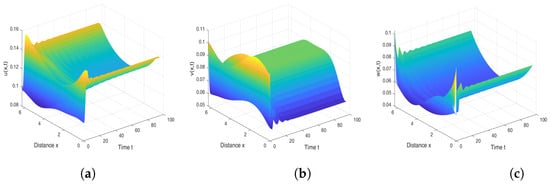
Figure 5. The spatiotemporal distribution of three populations of spatiotemporal model (3). (a) Susceptible prey. (b) Infected prey. (c) Predator. Here, parameter values are α = 8, β = 0.17, c = 0.004, γ = 10, d₁ = 0.25, d₂ = 0.2, d₃ = 5.2, q₁ = q₂ = 0.1, m = 0.6, n = 0.3, l = 0.5 and diffusion coefficients are D₁ = 0.1, D₂ = 0.1, D₃ = 20.

4. Discussion and Conclusions

On the basis of the model proposed in [16], we established a diffusion type predator–prey model for the spread of diseases within prey populations. In the model, we also considered the harvesting of prey and the negative effects of infected prey on predators. We conducted dynamic analysis and related numerical simulations on the temporal model (4) and spatiotemporal model (3). We hope that our theoretical and simulation results may explain some phenomena in nature.

For the temporal model (4), we verified the positivity and boundedness of the solution, studied the local stability of the model equilibrium point using eigenvalue analysis, and derived the conditions for the model to undergo Hopf bifurcation when a certain parameter changes. The analysis results indicate that the model has three feasible boundary equilibrium points and at most two positive equilibrium points. It is worth noting that when the harvesting intensity ${\displaystyle q_1}$ of susceptible prey exceeds a certain threshold, the dynamics undergo significant changes: only unstable extinction equilibrium ${\displaystyle E_0}$ and stable susceptible prey-only equilibrium ${\displaystyle E_1}$. This result suggests that overfishing of susceptible prey may lead to a chain extinction of infected prey and predator populations, which is consistent with the “fishing induced ecological cascade effect” proposed by Jackson et al. [35]. An interesting phenomenon was discovered through numerical simulation: increasing the fishing intensity of prey can effectively reduce the total density of the prey population (see Figure 1a), but the density of predators and susceptible prey actually shows an upward trend (see Figure 1b). The possible reason is that the reduction in infected prey alleviates the pressure of infection, allowing more susceptible individuals to survive and providing sufficient food sources for predators. Figure 1 simulates the impact of parameter ${\displaystyle n}$ variation on the biomass of three species. The results show that an increase in negative impact (n) leads to a decrease in predator density and an increase in prey density (see Figure 2a). At the same time, a decreasing trend in susceptible prey density is observed (see Figure 2b), which may be due to an increase in disease pressure caused by a decrease in predators. In terms of the periodic solutions of the model, infectivity (${\displaystyle \alpha }$) and harvest intensity (${\displaystyle q_1=q_2=q}$) have opposite effects on periodic oscillations (see Figure 3 and Figure 4). The increase in infection rate may lead to periodic fluctuations or even extinction of the population, while the increase in harvesting intensity may suppress this oscillation. This difference reflects the opposite regulatory effects of natural regulation (disease transmission) and human intervention (harvesting activities) on ecosystem stability, providing a new perspective for understanding the mechanisms of maintaining ecosystem stability.

For the spatiotemporal model (3), we employed the maximum principle and Harnack inequality to establish a priori estimates for the positive steady states of the corresponding elliptic system. Furthermore, using energy methods, we determined the conditions under which model (3) admits no non-constant steady states—indicating that rapid diffusion across all species may suppress the formation of spatially heterogeneous patterns. This is consistent with the research results in [36] and also in line with the “diffusion-driven homogenization” mechanism proposed by Okubo and Levin [37]. This finding aligns with previous studies (e.g., [36]) and supports the “diffusion-driven homogenization" mechanism proposed by Okubo and Levin [37]. Specifically, sufficiently fast diffusion promotes complete spatial mixing of populations, smoothing out local density variations and driving the system towards a uniform equilibrium. Further, by applying the Leray–Schauder degree theory, we derived sufficient conditions for the existence of nonhomogeneous positive steady states. Our results reveal that under certain parameter regimes, rapid predator diffusion (i.e., ${\displaystyle d_3}$ exceeding a critical threshold) can destabilize spatial homogeneity and induce pattern formation. This phenomenon is consistent with the diffusion-driven instability theory of Takaishi et al. [38], where enhanced predator mobility amplifies spatial heterogeneity in functional responses, disrupting uniform equilibria via a “predator-prey chase effect.” The rapid spread of predators leads to the gathering of infected prey in local areas, while susceptible prey forms safe zones by escaping, and infected individuals gather in space due to limited activity. This dynamic balance indicates that the rapid migration of predators often forms non-uniform distribution patterns, and also suggests that different diffusion patterns may play an important role in ecological models. The simulation results confirmed the existence of nonhomogeneous positive steady states (see Figure 5), and observed that susceptible prey and predators form high-density areas near the boundaries of the habitat, while infected prey forms high-density areas inside the habitat. The possible mechanism for the pattern formation is that boundary effects limit the escape of infected prey, and infected prey inside the habitat form high-density aggregation areas due to reduced predation pressure caused by limited mobility. At the same time, susceptible prey will actively migrate towards the boundary and form a coaggregation with predators to avoid disease transmission, reflecting the boundary refuge effect in this spatial self-organization pattern.

References

- Georgescu, P.; Hsieh, Y.H. Global dynamics of a predator-prey model with stage structure for the predator. SIAM J. Appl. Math. 2007, 67, 1379–1395. [Google Scholar] [CrossRef]
- Hsu, S.B.; Hwang, T.W.; Kuang, Y. Global dynamics of a predator-prey model with Hassell-Varley type functional response. Discret. Cont. Dyn-B 2008, 10, 857–871. [Google Scholar] [CrossRef]
- Chen, X.; Zhang, X. Dynamics of the predator-prey model with the Sigmiod functional response. Stud. Appl. Math. 2021, 147, 300–318. [Google Scholar] [CrossRef]
- Singh, M.K.; Sharma, A.; ánchez-Ruiz, L.M. Impact of the Allee effect on the dynamics of a predator-prey model exhibiting group defense. Mathematics 2025, 13, 633. [Google Scholar] [CrossRef]
- Ruan, S.; Zhao, X. Persistence and extinction in two species reaction-diffusion systems with delays. J. Differ. Equ. 1999, 156, 71–92. [Google Scholar] [CrossRef]
- Anderson, R.M.; May, R.M. The population dynamics of microparasites and their invertebrate hosts. Philos. T. R. Soc. B 1981, 291, 451–524. [Google Scholar]
- Jana, S.; Kar, T.K. Modeling and analysis of a prey-predator system with disease in the prey. Chaos, Soliton. Fract. 2013, 47, 42–53. [Google Scholar] [CrossRef]
- Chattopadhyay, J.; Ghosal, G.; Chaudhuri, K.S. Nonselective harvesting of a prey-predator community with infected prey. Korean J. Comput. Appl. Math. 1999, 6, 601–616. [Google Scholar] [CrossRef]
- Shaikh, A.A.; Das, H.; Sarwardi, S. Dynamics of an eco-epidemiological system with disease in competitive prey species. J. Appl. Math. Comput. 2020, 62, 525–545. [Google Scholar] [CrossRef]
- Xiao, Y.; Chen, L. A ratio-dependent predator-prey model with disease in the prey. Appl. Math. Comput. 2002, 131, 397–414. [Google Scholar] [CrossRef]
- Kabir, K.M.A. Mitigating infection in prey through cooperative behavior under fear-induced defense. Appl. Math. Comput. 2025, 495, 129318. [Google Scholar] [CrossRef]
- Haque, M. A predator-prey model with disease in the predator species only. Nonlinear Anal-Real. 2010, 11, 2224–2236. [Google Scholar] [CrossRef]
- Das, K.P. A study of chaotic dynamics and tts possible control in a predator-prey model with disease in the Predator. J. Dyn. Control Syst. 2015, 21, 605–624. [Google Scholar] [CrossRef]
- Kant, S.; Kumar, V. Stability analysis of predator-prey system with migrating prey and disease infection in both specise. Appl. Math. Model. 2017, 42, 509–539. [Google Scholar] [CrossRef]
- Gao, X.; Pan, Q.; He, M.; Kang, Y. A predator-prey model with diseases in both prey and predator. Physica A 2013, 392, 5898–5906. [Google Scholar] [CrossRef]
- Kar, T.K.; Ghorai, A.; Jana, S. Dynamics of pest and its predator model with disease in the pest and optimal use of pesticide. J. Theor. Biol. 2012, 310, 187–198. [Google Scholar] [CrossRef]
- Li, J.; Jin, Z.; Sun, G.Q.; Song, L.P. Pattern dynamics of a delayed eco-epidemiological model with disease in the predator. Discret. Contin. Dyn. Syst. Ser. S 2017, 10, 1025–1042. [Google Scholar] [CrossRef]
- Babakordi, N.; Zangeneh, H.R.Z.; Ghahfarokhi, M.M. Multiple bifurcation analysis in a diffusive eco-epidemiological model with time delay. Int. J. Bifurc. Chaos 2019, 29, 1–23. [Google Scholar] [CrossRef]
- Chakraborty, B.; Ghorai, S.; Bairag, N. Ghahfarokhi. Reaction-diffusion predator-prey-parasite system and spatiotemporal complexity. Appl. Math. Comput. 2020, 386, 125518. [Google Scholar]
- Melese, D.; Feyisa, S. Stability and bifurcation analysis of a diffusive modified Leslie- Gower prey-predator model with prey infection and Beddington DeAngelis functional response. Heliyon 2021, 7, e06193. [Google Scholar] [CrossRef]
- Vitanov, N.K.; Jordanov, I.P.; Dimitrova, Z.I. On nonlinear population waves. Appl. Math. Comput. 2009, 215, 2950–2964. [Google Scholar] [CrossRef]
- Hossain, S.; Haque, M.M.; Kabir, M.H.; Gani, M.O.; Sarwardi, S. Complex spatiotemporal dynamics of a harvested prey–predator model with Crowley–Martin response function. Results Control Optim. 2021, 50, 100059. [Google Scholar] [CrossRef]
- Sun, G.; Dai, B. Stability and bifurcation of a delayed diffusive predator-prey system with food-limited and nonlinear harvesting. Math. Biosci. Eng. 2020, 17, 3520–3552. [Google Scholar] [CrossRef] [PubMed]
- Xiao, D.; Jennings, L.S. Bifurcations of a ratio-dependent predator-prey system with constant rate harvesting. SIAM J. Appl. Math. 2005, 65, 737–753. [Google Scholar] [CrossRef]
- Xiao, D.; Li, W.; Han, M. Jennings, L.S. Dynamics in a ratio-dependent predator-prey model with predator harvesting. J. Math. Anal. Appl. 2006, 324, 14–29. [Google Scholar] [CrossRef]
- Bilu, E.; Coll, M. Parasitized aphids are inferior prey for a coccinellid predator: Implications for intraguild predation. Environ. Entom. 2009, 38, 153–158. [Google Scholar] [CrossRef]
- Forshay, K.J.; Johnson, P.T.; Stock, M.; Peñalva, C.; Dodson, S.I. Festering food: Chytridiomycete pathogen reduces quality of Daphnia host as a food resource. Ecology 2008, 89, 2692–2699. [Google Scholar] [CrossRef]
- Sures, B. How parasitism and pollution affect the physiological homeostasis of aquatic hosts. J. Helminthol. 2006, 80, 151–157. [Google Scholar] [CrossRef] [PubMed]
- Hadeler, K.P.; Freedman, H.I. Predator-prey populations with parasitic infection. J. Math. Biol. 1989, 27, 609–631. [Google Scholar] [CrossRef]
- Vitanov, N.K.; Jordanov, I.P.; Dimitrova, Z.I. On nonlinear dynamics of interacting populations: Coupled kink waves in a system of two populations. Commun. Nonlinear SCI. 2009, 14, 2379–2388. [Google Scholar] [CrossRef]
- Lou, Y.; Ni, W.M. Diffusion, self-diffusion and cross-diffusion. J. Differ. Equ. 1996, 131, 79–131. [Google Scholar] [CrossRef]
- Lou, C.S.; Ni, W.M.; Takage, I. Large amplitude ststionary solutions to a chemotaxis system. J. Differ. Equ. 1998, 72, 1–27. [Google Scholar]
- Nirenberg, L. Topics in Nonlinear Functional Analusis; American Mathematical Society: Providence, RI, USA, 2001. [Google Scholar]
- Peng, R.; Shi, J.; Wang, M. Stationary pattern of a ratio-dependent food chain model with diffusion. SIAM J. Appl. Math. 2007, 67, 1479–1503. [Google Scholar] [CrossRef]
- Jackson, J.B.; Kirby, M.X.; Berger, W.H.; Bjorndal, K.A.; Botsford, L.W.; Bourque, B.J.; Bradbury, R.H.; Cooke, R.; Erlson, J.; Estes, J.A.; et al. Historical overfishing and the recent collapse of coastal ecosystems. Science 2001, 293, 629–637. [Google Scholar] [CrossRef]
- Conway, E.; Hoff, D.; Smoller, J. Large time behavior of solutions of systems of nonlinear reaction-diffusion equations. SIAM J. Appl. Math. 1978, 35, 1–16. [Google Scholar] [CrossRef]
- Okubo, A.; Levin, S.A. Diffusion and Ecological Problems: Modern Perspectives; Springer Science and Business Media: Berlin/Heidelberg, Germany, 2002. [Google Scholar]
- Takaishi, T.; Mimura, M.; Nishiura, Y. Pattern formation in coupled reaction-diffusion systems. Jap. J. Appl. Math. 1995, 12, 385–424. [Google Scholar] [CrossRef][Green Version]
Disclaimer/Publisher’s Note: The statements, opinions and data contained in all publications are solely those of the individual author(s) and contributor(s) and not of MDPI and/or the editor(s). MDPI and/or the editor(s) disclaim responsibility for any injury to people or property resulting from any ideas, methods, instructions or products referred to in the content. |
© 2025 by the authors. Licensee MDPI, Basel, Switzerland. This article is an open access article distributed under the terms and conditions of the Creative Commons Attribution (CC BY) license (https://creativecommons.org/licenses/by/4.0/).