A Novel Recursive Algorithm for Inverting Matrix Polynomials via a Generalized Leverrier–Faddeev Scheme: Application to FEM Modeling of Wing Vibrations in a 4th-Generation Fighter Aircraft

Abstract

This paper introduces a novel recursive algorithm for inverting matrix polynomials, developed as a generalized extension of the classical Leverrier–Faddeev scheme. The approach is motivated by the need for scalable and efficient inversion techniques in applications such as system analysis, control, and FEM-based structural modeling, where matrix polynomials naturally arise. The proposed algorithm is fully numerical, recursive, and division free, making it suitable for large-scale computation. Validation is performed through a finite element simulation of the transverse vibration of a fighter aircraft wing. Results confirm the method’s accuracy, robustness, and computational efficiency in computing characteristic polynomials and adjugate-related forms, supporting its potential for broader application in control, structural analysis, and future extensions to structured or nonlinear matrix systems.

1. Introduction

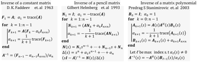
The study of matrix inversion ${\mathit{A}}^{-1}\in {\mathbb{C}}^{n\times n}$ and matrix polynomial inversion ${\mathit{A}}^{-1}\left(\lambda \right)\in {\mathbb{C}}^{n\times n}\left[\lambda \right]$ has been a central topic in computational linear algebra, motivating extensive research over several decades. Early developments include Frame’s (1949) recursive formula for computing matrix inverses [1], Davidenko’s (1960) method based on variation of parameters [2], and Gantmacher’s foundational work on matrix theory [3]. Between 1961 and 1964, Lancaster made key contributions to nonlinear matrix problems, algorithms for λ-matrices, and generalized Rayleigh quotient methods for eigenvalue problems [4,5,6]. Significant progress was made by Faddeev and Faddeeva (1963–1975) in computational techniques [7], and Householder’s monograph [8] became a standard reference. In parallel, Decell (1965) employed the Cayley–Hamilton theorem for generalized inversion [9], forming a basis for later extensions to polynomial matrices. In the 1980s, Givens proposed modifications to the classical Leverrier–Faddeev algorithm [10], while Paraskevopoulos (1983) introduced Chebyshev-based methods for system analysis and control [11], enriching the theory of polynomial matrix inversion.

Barnett, in 1989, provided a new proof and important extensions of the Leverrier–Faddeev algorithm, introducing computational schemes for matrix polynomials of degree two $\mathit{A}\left(\lambda \right)={\lambda }^2{\mathit{I}}_n+\lambda {\mathit{A}}_1+{\mathit{A}}_2$ [12]. In the 1990s, Fragulis and collaborators (1991) addressed the inversion of polynomial matrices and their Laurent expansions [13], while Fragulis (1995) established a generalized Cayley–Hamilton theorem for polynomial matrices of arbitrary degree [14]. In 1993, Helmberg, Wagner, and Veltkamp revisited the Leverrier–Faddeev method, focusing on characteristic polynomials and eigenvectors [15]. Wang and Lin (1993) proposed an extension of the Leverrier algorithm for higher-degree matrix polynomials [16], although practical implementation remained limited. Further developments included Hou, Pugh, and Hayton (2000), who proposed a general solution for systems in polynomial matrix form [17], and Djordjevic (2001), who investigated generalized Drazin inverses [18]. Debeljković (2004) contributed to the theory of singular control systems [19]. Hernández (2004) introduced an extension of the Leverrier–Faddeev algorithm using bases of classical orthogonal polynomials [20], offering improved flexibility in polynomial matrix inversion. In parallel, Stanimirovic and his collaborators, between 2006 and 2011, initiated a series of extensions of the Leverrier–Faddeev algorithm toward generalized inverses and rational matrices, culminating in multiple key contributions across the 2000s [21,22,23,24,25,26], providing practical and effective computational algorithms. Petkovic (2006) further developed interpolation-type algorithms related to the Leverrier–Faddeev method [27]. Recent efforts expanded the theory toward modern applications. In 2019, Dopico introduced the concept of root polynomials and their role in matrix polynomial theory [28]. In 2021, Tian and Xia studied low-degree solutions for the Sylvester matrix polynomial equation [29], while Shehata (2021) addressed Lommel matrix polynomials [30]. In 2024, significant theoretical expansions were presented: Szymański explored stability theory for matrix polynomials [31]; Kumar proposed numerical methods for exploring zeros of Hermite-lambda matrix polynomials [32]; Zainab studied symbolic approaches for Appell-lambda matrix families [33]; and Milica investigated the implications of higher-degree polynomials in forced damped oscillations [34]. Halidias (2024) also contributed novel methods for minimum polynomial computations [35]. Overall, the evolution of matrix polynomial inversion, the Leverrier–Faddeev method, and associated generalized inversion techniques has grown from classical recursion-based strategies to sophisticated symbolic, interpolation, and numerical algorithms, addressing the challenges posed by high-degree, singular, or rational polynomial matrices.

This work is motivated by the need for more efficient and straightforward algorithms to compute matrix polynomial inverses, particularly for large-scale systems. Existing Leverrier–Faddeev-based methods often suffer from high computational complexity and limited applicability to higher-degree polynomials and multivariable transfer functions. The proposed recursive algorithm itself constitutes a major innovation, offering a simple and efficient solution. It also extends naturally to companion forms and descriptor systems, areas not fully explored in previous methods. Furthermore, the algorithm can handle non-regular and potentially rational matrix polynomials, addressing a significant gap in the literature. This work thus provides a powerful tool for efficient matrix polynomial inversion with broad applications in system analysis and control.

In this paper, we present a new and efficient scheme for computing the inverse of matrix polynomials of arbitrary degree. The paper is organized as follows: Section 2 introduces the necessary preliminaries. In Section 3, we formulate the problem statement and discuss classical algorithms. Section 4 presents our main algorithm, and Section 5 explores its connection to companion forms. Section 6 extends the method to descriptor systems, while Section 7 demonstrates the application of our approach through practical simulations. Finally, Section 8 concludes this paper.

2. Preliminaries on Matrix Functions

Now, we introduce matrix functions, highlight their key properties and importance in system theory, and lay the foundation for their application in system analysis.

2.1. Matrix Functions by the Sylvester Formula

The term “function of a matrix” can have several different meanings. In this monograph, we are interested in a definition that takes a scalar function f and a matrix $\mathit{A}\in {\mathbb{C}}^{n\times n}$ and specifies $\mathrm{f}\left(\mathit{A}\right)$ to be a matrix of the same dimensions as $\mathit{A}$; it does so in a way that provides a useful generalization of the function of a scalar variable $\mathrm{f}\left(z\right)$, $z\in \mathbb{C}$. Other interpretations of $\mathrm{f}\left(\mathit{A}\right)$ are: functions mapping ${\mathbb{C}}^{n\times n}$ to ${\mathbb{C}}^{m\times m}$ that do not stem from a scalar function. Examples include matrix polynomials $\mathit{A}\left(\lambda \right)\in {\mathbb{C}}^{n\times n}\left[\lambda \right]$ with matrix coefficients, the matrix transpose, the $\mathrm{adjugate}$ (or $\mathrm{adjoint}$) matrix, compound matrices comprising minors of a given matrix, and factors from matrix factorizations and as a special case, the polar factors of a matrix. Another example is the elementwise operations on matrices, for example $\sin \left(\mathit{A}\right)=\left(\sin \left(a_{ij}\right)\right)$. In addition, there are functions that produce a scalar result, such as the trace, the determinant, the spectral radius, the condition number $\kappa \left(\mathit{A}\right)$, and one particular generalization to matrix arguments of the hypergeometric function. The Sylvester formula is an identity that can provide matrix function evaluation using the projectors $G_i \left(\mathrm{or} Z_{ij}\right)$, minimal polynomial and the Lagrange interpolation techniques. In this section, we will explore how it is applied.

Theorem 1.

(Functions of non-diagonalizable matrices) If  $\mathit{A}\in {\mathbb{C}}^{n\times n}$ with a spectrum  $\sigma \left(\mathit{A}\right)={\lambda }_1, {\lambda }_2, \dots , {\lambda }_s$, let  $k_i=\mathrm{index}\left({\lambda }_i\right)$. A function  $\mathrm{f} : \mathbb{C}\to \mathbb{C}$  is said to be defined (or to exist) at  $\mathit{A}$  when  $\mathrm{f}\left({\lambda }_i\right)$, ${\mathrm{f}}^{\left(1\right)}\left({\lambda }_i\right)$, $\dots$, ${\mathrm{f}}^{\left(k_i-1\right)}\left({\lambda }_i\right)$  exist for each  ${\lambda }_i\in \sigma \left(\mathit{A}\right)$. The value of  $\mathrm{f}\left(\mathit{A}\right)$  is:

$$\mathrm{f}\left(\mathit{A}\right)=\underset{i=1}{\overset{s}{⅀}}\underset{j=0}{\overset{k_i-1}{⅀}}{\mathrm{f}}^{\left(j\right)}\left({\lambda }_i\right) {\displaystyle \frac{{\left(\mathit{A}-{\lambda }_i\mathit{I}\right)}^j{\mathit{G}}_i}{j!}}=\underset{i=1}{\overset{s}{⅀}}\underset{j=0}{\overset{k_i-1}{⅀}}{\mathrm{f}}^{\left(j\right)}\left({\lambda }_i\right) Z_{ij}$$

(1)

Proof: 

Let $\sigma \left(\mathit{A}\right)=\left\{{\lambda }_1, {\lambda }_2,\dots ,{\lambda }_s\right\}\subset \mathbb{C}$ be a set of $s$ (distinct) eigenvalues of diagonalizable matrix $\mathit{A}$ and $\mathrm{f}$ be a function defined on the spectrum of $\mathit{A}$. Let the polynomial function $p\left(\lambda \right)={⅀}_{k=0}^n{c}_k{\lambda }^k={ℿ}_{i=1}^s{\left(\lambda -{\lambda }_i\right)}^{m_i}$ be the characteristic polynomial of $\mathit{A}$. The minimal polynomial of $\mathit{A}$ is given by $\psi \left(\lambda \right)={ℿ}_{i=1}^s{\left(\lambda -{\lambda }_i\right)}^{{\mathrm{g}}_i}$ with $1\le {\mathrm{g}}_i\le m_i$ but because of the diagonalizability of $\mathit{A}$, we have ${\mathrm{g}}_i=1$, hence $\psi \left(\lambda \right)={ℿ}_{i=1}^s\left(\lambda -{\lambda }_i\right)$, which is of degree $s$. Now let us prove that there exists a unique polynomial $r\left(\lambda \right)={⅀}_{k=0}^{s-1}{\alpha }_k{\lambda }^k$ of degree $s-1$ such that $\mathrm{f}\left({\lambda }_i\right)=r\left({\lambda }_i\right)={⅀}_{k=0}^{s-1}{\alpha }_k{\lambda }_i^k \mathrm{for} i=1,2, \dots , \mathrm{s}$. To prove this claim, let us write the last formula in matrix form so we have

$$\left(\begin{array}{cc}\begin{array}{cc}\begin{array}{c}1\\ \begin{array}{c}1\\ ⋮\end{array}\\ 1\end{array}& \begin{array}{cc}\begin{array}{c}{\lambda }_1\\ \begin{array}{c}{\lambda }_2\\ ⋮\end{array}\\ {\lambda }_s\end{array}& \begin{array}{c}{\lambda }_1^2\\ \begin{array}{c}{\lambda }_2^2\\ ⋮\end{array}\\ {\lambda }_s^2\end{array}\end{array}\end{array}& \begin{array}{cc}\begin{array}{c}\begin{array}{c}\dots \\ \end{array}\\ \begin{array}{c}\dots \\ \begin{array}{c}⋮\\ \end{array}\end{array}\\ \dots \end{array}& \begin{array}{c}{\lambda }_1^{s-1}\\ \begin{array}{c}{\lambda }_2^{s-1}\\ ⋮\end{array}\\ {\lambda }_s^{s-1}\end{array}\end{array}\end{array}\right)\left(\begin{array}{c}{\alpha }_0\\ \begin{array}{c}\begin{array}{c}{\alpha }_1\\ {\alpha }_2\end{array}\\ ⋮\end{array}\\ {\alpha }_{s-1}\end{array}\right)=\left(\begin{array}{c}\mathrm{f}\left({\lambda }_1\right)\\ \begin{array}{c}\begin{array}{c} \\ \end{array}\\ ⋮\end{array}\\ \mathrm{f}\left({\lambda }_s\right)\end{array}\right) ⟺ \mathit{V}\mathsf{\alpha }=f$$

(2)

This system has a unique solution if and only if the determinant of the Vandermonde matrix $\mathit{V}$ does not vanish $\det \left(\mathit{V}\left({\lambda }_1, \dots ,{\lambda }_s\right)\right)\ne 0$. It is not difficult to verify that $\det \left(\mathit{V}\left({\lambda }_1, \dots ,{\lambda }_s\right)\right)={ℿ}_{0\le i<j\le s}\left({\lambda }_j-{\lambda }_i\right)$. Hence, since the points are pairwise distinct, the determinant does not vanish. Computing the solution of the system, we get

$$\mathsf{\alpha }={\mathit{V}}^{-1}f ⟺ \left(\begin{array}{c}{\alpha }_0\\ \begin{array}{c}\begin{array}{c}{\alpha }_1\\ {\alpha }_2\end{array}\\ ⋮\end{array}\\ {\alpha }_{s-1}\end{array}\right)=\left(\begin{array}{cc}\begin{array}{cc}\begin{array}{c}{\mathit{\ell }}_{11}\\ \begin{array}{c}{\mathit{\ell }}_{12}\\ ⋮\end{array}\\ {\mathit{\ell }}_{1s}\end{array}& \begin{array}{c}{\mathit{\ell }}_{21}\\ \begin{array}{c}{\mathit{\ell }}_{22}\\ ⋮\end{array}\\ {\mathit{\ell }}_{2s}\end{array}\end{array}& \begin{array}{cc}\begin{array}{c}\dots \\ \begin{array}{c}\dots \\ \begin{array}{c}⋮\\ \end{array}\end{array}\\ \dots \end{array}& \begin{array}{c}{\mathit{\ell }}_{s1}\\ \begin{array}{c}{\mathit{\ell }}_{s2}\\ ⋮\end{array}\\ {\mathit{\ell }}_{ss}\end{array}\end{array}\end{array}\right)\left(\begin{array}{c}\mathrm{f}\left({\lambda }_1\right)\\ \begin{array}{c}\begin{array}{c} \\ \end{array}\\ ⋮\end{array}\\ \mathrm{f}\left({\lambda }_s\right)\end{array}\right) ⟺ {\alpha }_{k-1}=\underset{i=1}{\overset{s}{⅀}}{\mathit{\ell }}_{ik}\mathrm{f}\left({\lambda }_i\right)$$

(3)

Such that when we make a substitution of ${\alpha }_{k-1}$ into $r\left(\lambda \right)$, we obtain

$$r\left(\lambda \right)=\underset{j=1}{\overset{s}{⅀}}{\alpha }_{j-1}{\lambda }^{j-1}=\underset{j=1}{\overset{s}{⅀}}\underset{i=1}{\overset{s}{⅀}}{\mathit{\ell }}_{ij}\mathrm{f}\left({\lambda }_i\right){\lambda }^{j-1}=\underset{i=1}{\overset{s}{⅀}}\mathrm{f}\left({\lambda }_i\right)\left({⅀}_{j=1}^s{\mathit{\ell }}_{ij}{\lambda }^{j-1}\right)=\underset{i=1}{\overset{s}{⅀}}\mathrm{f}\left({\lambda }_i\right)L_i\left(\lambda \right)$$

(4)

Note that the inverse of the Vandermonde matrix $\mathit{V}$ has as its columns the coefficients of the Lagrange interpolation polynomials. In other words, the inverse of $\mathit{V}$ results in the coefficients of the Lagrange interpolation polynomials. According to Lagrange interpolation method, we have

$$r\left(\lambda \right)={⅀}_{i=1}^s\mathrm{f}\left({\lambda }_i\right)L_i\left(\lambda \right) \mathrm{with} L_i\left(\lambda \right)={⅀}_{j=1}^s{\mathit{\ell }}_{ij}{\lambda }^{j-1}$$

(5)

where Cramer’s rules results in

$$r\left(\lambda \right)=\underset{i=1}{\overset{s}{⅀}}\mathrm{f}\left({\lambda }_i\right)L_i\left(\lambda \right)=\underset{i=1}{\overset{s}{⅀}}\mathrm{f}\left({\lambda }_i\right){\displaystyle \frac{\det \left[\mathit{V}\left({\lambda }_1, \dots ,{\lambda }_{i-1},\lambda ,{\lambda }_{i+1},\dots ,{\lambda }_s\right)\right]}{\det \left[\mathit{V}\left({\lambda }_1, . . . ,{\lambda }_s\right)\right]}}=\underset{i=1}{\overset{s}{⅀}}\mathrm{f}\left({\lambda }_i\right)\underset{\underset{j\ne i}{i=1}}{\overset{s}{ℿ}}{\displaystyle \frac{\lambda -{\lambda }_j}{{\lambda }_i-{\lambda }_j}}$$

(6)

Therefore, from the Lagrange interpolation polynomials, we get the Sylvester formula

$$\mathrm{f}\left(\mathit{A}\right)=r\left(\mathit{A}\right)=\underset{i=1}{\overset{s}{⅀}}\mathrm{f}\left({\lambda }_i\right)\underset{\underset{j\ne i}{i=1}}{\overset{s}{ℿ}}{\displaystyle \frac{\left(\mathit{A}-{\lambda }_j\mathit{I}\right)}{\left({\lambda }_i-{\lambda }_j\right)}}=\underset{i=1}{\overset{s}{⅀}}\mathrm{f}\left({\lambda }_i\right)G_i, \mathrm{with} G_i=\underset{\underset{j\ne i}{i=1}}{\overset{s}{ℿ}}{\displaystyle \frac{\left(\mathit{A}-{\lambda }_j\mathit{I}\right)}{\left({\lambda }_i-{\lambda }_j\right)}}$$

(7)

In the case of non-diagonalizable matrices $\mathrm{index}\left({\lambda }_i\right)=k_i\ne 1$, we can generalize the previous result to, so we have (see [36])

$$\mathrm{f}\left(\mathit{A}\right)=\underset{i=1}{\overset{s}{⅀}}\underset{j=0}{\overset{k_i-1}{⅀}}{\mathrm{f}}^{\left(j\right)}\left({\lambda }_i\right) {\displaystyle \frac{{\left(\mathit{A}-{\lambda }_i\mathit{I}\right)}^j{G}_i}{j!}}=\underset{i=1}{\overset{s}{⅀}}\underset{j=0}{\overset{k_i-1}{⅀}}{\mathrm{f}}^{\left(j\right)}\left({\lambda }_i\right) Z_{ij} \mathrm{where} Z_{ij}={\displaystyle \frac{{\left(\mathit{A}-{\lambda }_i\mathit{I}\right)}^j{G}_i}{j!}}$$

(8)

$Z_{ij}$ is often called the component matrices or the constituent matrices. □

2.2. The Matrix Cauchy Integral Formula

The matrix Cauchy integral formula is an elegant result from complex analysis (and functional calculus), stating that if $\mathrm{f}:\mathbb{C}\to \mathbb{C}$ is analytic in and on a simple closed contour $\mathit{\Gamma }\subset \mathbb{C}$ with positive (counterclockwise) orientation, and if $\lambda$ is interior to $\mathit{\Gamma }$, then

$$\mathrm{f}\left(\lambda \right)={\displaystyle \frac{1}{2\pi j}}{{\displaystyle \oint }}_{\mathit{\Gamma }}{\displaystyle \frac{\mathrm{f}\left(z\right)}{z-\lambda }}dz \mathrm{and} {\mathrm{f}}^{\left(k\right)}\left(\lambda \right)={\displaystyle \frac{k!}{2\pi j}}{{\displaystyle \oint }}_{\mathit{\Gamma }}{\displaystyle \frac{\mathrm{f}\left(z\right)}{{\left(z-\lambda \right)}^{k+1}}}dz$$

(9)

These formulas produce analogous representations of matrix functions. Suppose that $\mathit{A}\in {\mathbb{C}}^{n\times n}$ with $\sigma \left(\mathit{A}\right)=\left\{{\lambda }_1, {\lambda }_2,\dots ,{\lambda }_s\right\}$, let the $\mathrm{index}\left({\lambda }_i\right)=k_i$. For a complex variable $\mu$, the resolvent of $\mathit{A}\in {\mathbb{C}}^{n\times n}$ is defined to be the matrix ${\mathit{R}}_{\mathit{A}}\left(\mu \right)={\left(\mu \mathit{I}-\mathit{A}\right)}^{-1}$. If we assume that $\mu \notin \sigma \left(\mathit{A}\right)$, and define the complex scalar function $r\left(z\right)={\left(\mu -z\right)}^{-1}$, then the evaluation of $r\left(z\right)$ at $\mathit{A}$ is given by $\mathit{r}\left(\mathit{A}\right)={\mathit{R}}_{\mathit{A}}\left(\mu \right)$, so the spectral resolution theorem can be used to write (Partial Fraction Expansion of ${\mathit{R}}_{\mathit{A}}\left(\mu \right)$)

$$\mathit{r}\left(\mathit{A}\right)={\left(\mu \mathit{I}-\mathit{A}\right)}^{-1}=\underset{i=1}{\overset{s}{⅀}}\underset{k=0}{\overset{k_i-1}{⅀}}{\displaystyle \frac{ r^{\left(k\right)}\left({\lambda }_i\right)}{k!}}{\left(\mathit{A}-{\lambda }_i\mathit{I}\right)}^k{G}_i =\underset{i=1}{\overset{s}{⅀}}\underset{k=0}{\overset{k_i-1}{⅀}}{\displaystyle \frac{ {\left(\mathit{A}-{\lambda }_i\mathit{I}\right)}^k{G}_i}{{\left(\mu -{\lambda }_i\right)}^{k+1}}}$$

(10)

If $\sigma \left(\mathit{A}\right)$ is in the interior of a simple closed contour $\mathit{\Gamma }$, and if the contour integral of a matrix is defined by $\mathrm{entrywise}$ integration, then complex integration gives

$${\displaystyle \frac{1}{2\pi j}}{{\displaystyle \oint }}_{\mathit{\Gamma }}\mathrm{f}\left(\mu \right){\mathit{R}}_{\mathit{A}}\left(\mu \right)d\mu ={\displaystyle \frac{1}{2\pi j}}{{\displaystyle \oint }}_{\mathit{\Gamma }}\mathrm{f}\left(\mu \right){\left(\mu \mathit{I}-\mathit{A}\right)}^{-1}d\mu ={\displaystyle \frac{1}{2\pi j}}{{\displaystyle \oint }}_{\mathit{\Gamma }}\mathrm{f}\left(\mu \right)\underset{i=1}{\overset{s}{⅀}}\underset{k=0}{\overset{k_i-1}{⅀}}{\displaystyle \frac{ {\left(\mathit{A}-{\lambda }_i\mathit{I}\right)}^k{G}_i}{{\left(\mu -{\lambda }_i\right)}^{k+1}}}d\mu$$

(11)

$$\left(11\right)\iff \underset{i=1}{\overset{s}{⅀}}\underset{k=0}{\overset{k_i-1}{⅀}}\left\{{\displaystyle \frac{1}{2\pi j}}{{\displaystyle \oint }}_{\mathit{\Gamma }}{\displaystyle \frac{\mathrm{f}\left(\mu \right)}{{\left(\mu -{\lambda }_i\right)}^{k+1}}}d\mu \right\}{\left(\mathit{A}-{\lambda }_i\mathit{I}\right)}^k{G}_i=\underset{i=1}{\overset{s}{⅀}}\underset{k=0}{\overset{k_i-1}{⅀}}{\displaystyle \frac{{\mathrm{f}}^{\left(k\right)}\left({\lambda }_i\right)}{k!}}{\left(\mathit{A}-{\lambda }_i\mathit{I}\right)}^k{G}_i$$

(12)

According to the spectral resolution theorem, we deduce that whenever $\mathrm{f}$ is analytic in and on a simple closed contour $\mathit{\Gamma }$ containing $\sigma \left(\mathit{A}\right)$ in its interior then

$$\mathrm{f}\left(\mathit{A}\right)={\displaystyle \frac{1}{2\pi j}}{{\displaystyle \oint }}_{\mathit{\Gamma }}\mathrm{f}\left(\mu \right){\left(\mu \mathit{I}-\mathit{A}\right)}^{-1}d\mu$$

(13)

Furthermore, if ${\mathit{\Gamma }}_i$ is a simple closed contour enclosing ${\lambda }_i$ but excluding all other eigenvalues of $\mathit{A}$, then the $i^{th}$ spectral projector can be obtained from

$$\mathrm{f}\left(z\right)=1 \forall z\in \mathbb{C} ⟺ \mathrm{f}\left(\mathit{A}\right)={\displaystyle \frac{1}{2\pi j}}{{\displaystyle \oint }}_{\mathit{\Gamma }}{\left(\mu \mathit{I}-\mathit{A}\right)}^{-1}d\mu ={\displaystyle \frac{1}{2\pi j}}\left[\underset{i=1}{\overset{s}{⅀}}{{\displaystyle \oint }}_{{\mathit{\Gamma }}_i}{\left(\mu \mathit{I}-\mathit{A}\right)}^{-1}d\mu \right]=\mathit{I}$$

(14)

On the other hand, we know that $\mathit{I}=G_1⨁G_2⨁ \cdots ⨁G_{\mathrm{s}}$, that is

$$G_i={\displaystyle \frac{1}{2\pi j}}{{\displaystyle \oint }}_{{\mathit{\Gamma }}_i}{\left(\mu \mathit{I}-\mathit{A}\right)}^{-1}d\mu ={{\displaystyle \oint }}_{{\mathit{\Gamma }}_i}{\displaystyle \frac{{\mathit{R}}_{\mathit{A}}\left(\mu \right)}{2\pi j}}d\mu$$

(15)

Other types of functions we consider are those which include mapping from $\mathbb{C}$ to ${\mathbb{C}}^{n\times n}$, such as the matrix transfer function $\mathit{H}\left(\lambda \right)=\mathit{B}{\left(\lambda \mathit{I}-\mathit{A}\right)}^{-1}\mathit{C}$, for $\mathit{B}\in {\mathbb{C}}^{n\times m}$, $\mathit{A}\in {\mathbb{C}}^{n\times n}$, and $\mathit{C}\in {\mathbb{C}}^{m\times n}$ (as discussed by Oskar Jakub Szymański [31] and Higham, Nicholas, Lucian Milica [34,35,36]). An alternative reformulation of $\mathit{H}\left(\lambda \right)\in {\mathbb{C}}^{n\times n}\left[\lambda \right]$ will produce the following matrix fraction description $\mathit{H}\left(s\right)=\mathit{N}\left(\lambda \right){\mathit{D}}^{-1}\left(\lambda \right)$, so in this context and as a special work, we are interested by the computation of such matrix function.

2.3. The Role of the Resolvent

The quantity $\mathit{A}\left(\lambda \right)=\lambda \mathit{I}-\mathit{A}$ is the called first-order matrix polynomial or the linearized form (some authors refers this as pencil linearization). The inverse of this quantity is a fundamental estimate known as the resolvent matrix ${\mathit{R}}_{\mathit{A}}\left(\lambda \right)={\left(\lambda \mathit{I}-\mathit{A}\right)}^{-1}$ as mentioned before. The resolvent is a central object in spectral theory—it reveals the existence of eigenvalues, indicates where eigenvalues can fall, and shows how sensitive these eigenvalues are to perturbations. As the inverse of the matrix ${\left(\mu \mathit{I}-\mathit{A}\right)}^{-1}$, the resolvent will have as its entries rational functions of $\lambda$. The resolvent fails to exist at any $\lambda \in \sigma \left(\mathit{A}\right)$. To better appreciate its nature, consider a simple example

$$\mathit{A}=\left(\begin{array}{cc}2& -2\\ 1& -1\end{array}\right) ⟹ {\mathit{R}}_{\mathit{A}}\left(\lambda \right)={\left(\lambda \mathit{I}-\mathit{A}\right)}^{-1}={\left(\begin{array}{cc}\lambda -2& 2\\ -1& \lambda +1\end{array}\right)}^{-1}={\displaystyle \frac{1}{\lambda \left(\lambda -1\right)}}\left(\begin{array}{cc}\lambda +1& -2\\ 1& \lambda -2\end{array}\right)$$

Being comprised of rational functions, the resolvent has a complex derivative at any point $\lambda \in \mathbb{C}$ that is not in $\sigma \left(\mathit{A}\right)$, and hence on any open set in the $\mathbb{C}$ not containing an eigenvalue, the resolvent is an analytic function. Suppose that we have $\mathit{A}\in {\mathbb{C}}^{n\times n}$ with $\sigma \left(\mathit{A}\right)=\left\{{\lambda }_1, {\lambda }_2,\dots ,{\lambda }_s\right\}$, and the $\mathrm{index}\left({\lambda }_i\right)=k_i=1$.

$${\mathit{R}}_{\mathit{A}}\left(\lambda \right)={\left(\lambda \mathit{I}-\mathit{A}\right)}^{-1}=\underset{i=1}{\overset{s}{⅀}}\underset{K=0}{\overset{k_i-1}{⅀}}{\displaystyle \frac{ {\left(\mathit{A}-{\lambda }_i\mathit{I}\right)}^k{G}_i}{{\left(\lambda -{\lambda }_i\right)}^{k+1}}}=\underset{i=1}{\overset{s}{⅀}}{\left(\lambda -{\lambda }_i\right)}^{-1}{G}_i$$

(16)

Moreover, the eigenvalues of ${\left(\lambda \mathit{I}-\mathit{A}\right)}^{-1}$ are ${\left(\lambda -{\lambda }_i\right)}^{-1}$ because

$${\mathit{R}}_{\mathit{A}}\left(\lambda \right)={\left(\lambda \mathit{I}-\mathit{A}\right)}^{-1}={\left[\lambda \underset{i=1}{\overset{s}{⅀}}{G}_i-\underset{i=1}{\overset{s}{⅀}}{\lambda }_i{G}_i\right]}^{-1}={\left[\underset{i=1}{\overset{s}{⅀}}\left(\lambda -{\lambda }_i\right)G_i\right]}^{-1}=\underset{i=1}{\overset{s}{⅀}}{\left(\lambda -{\lambda }_i\right)}^{-1}{G}_i$$

(17)

Theorem 2.

The resolvent  ${\mathit{R}}_{\mathit{A}}\left(\lambda \right)$ of $\mathit{A}\in {\mathbb{C}}^{n\times n}$ is a rational function of $\lambda$ with poles at the points of the spectrum of A. Moreover, each ${\lambda }_i\in \sigma \left(\mathit{A}\right)$ is a pole of ${\mathit{R}}_{\mathit{A}}\left(\lambda \right)$ of algebraic multiplicity $m_i$, (${⅀}_{i=1}^s{m}_i=n$), that is

$${\mathit{R}}_{\mathit{A}}\left(\lambda \right)={\left(\lambda \mathit{I}-\mathit{A}\right)}^{-1}={\displaystyle \frac{1}{p\left(\lambda \right)}}\underset{j=1}{\overset{s}{⅀}}\underset{i=1}{\overset{s}{⅀}}{\gamma }_{ij}{\lambda }^i{\mathit{A}}^j \mathrm{with} p\left(\lambda \right)=\underset{i=1}{\overset{s}{ℿ}}{\left(\lambda -{\lambda }_i\right)}^{m_i}$$

(18)

Proof: 

Evidently $\left[p\left(\lambda \right)-p\left(\mu \right)\right]=\left[{⅀}_{j=1}^s{⅀}_{i=1}^s{\gamma }_{ij}{\lambda }^i{\mu }^j\right]\left(\lambda -\mu \right)$ for some numbers ${\gamma }_{ij}$. Using the matrix polynomial definition (as in the Cayley–Hamilton theorem) for ${\lambda }_i\notin \sigma \left(\mathit{A}\right)$ the last relation (after formal substituting $\mathit{A}$ for $\mu$) implies

$$\left(p\left(\lambda \right)\mathit{I}-p\left(\mathit{A}\right)\right){\left(\lambda \mathit{I}-\mathit{A}\right)}^{-1}=\left[\underset{j=1}{\overset{s}{⅀}}\underset{i=1}{\overset{s}{⅀}}{\gamma }_{ij}{\lambda }^i{\mathit{A}}^j\right] ⟹ {\mathit{R}}_{\mathit{A}}\left(\lambda \right)={\displaystyle \frac{1}{p\left(\lambda \right)}}\left[\underset{j=1}{\overset{s}{⅀}}\underset{i=1}{\overset{s}{⅀}}{\gamma }_{ij}{\lambda }^i{\mathit{A}}^j\right]$$

(19)

Since by the Cayley–Hamilton theorem $p\left(\mathit{A}\right)=\mathbf{0}$ □

Properties of Matrix Resolvents:

$$\begin{array}{l}• {\mathit{R}}_{\mathit{A}}\left(\lambda \right)={\displaystyle \frac{1}{p\left(\lambda \right)}}{⅀}_{j=1}^s\left({⅀}_{i=1}^s{\gamma }_{ij}{\lambda }^i\right){\mathit{A}}^j\\ • {\mathit{R}}_{\mathit{A}}\left(\lambda \right)={⅀}_{i=1}^s{⅀}_{k=0}^{k_i-1}{\displaystyle \frac{ {\left(\mathit{A}-{\lambda }_i\mathit{I}\right)}^k{G}_i}{{\left(\mu -{\lambda }_i\right)}^{k+1}}}\\ • {\displaystyle \frac{1}{2\pi j}}{{\displaystyle \oint }}_{\mathit{\Gamma }}{\mathit{R}}_{\mathit{A}}\left(\mu \right)d\mu =\mathit{I}\end{array}$$

$$\begin{array}{l}• {\mathit{R}}_{\mathit{A}}\left(\lambda \right)-{\mathit{R}}_{\mathit{A}}\left(\mu \right)=\left(\lambda -\mu \right){\mathit{R}}_{\mathit{A}}\left(\lambda \right){\mathit{R}}_{\mathit{A}}\left(\mu \right)\\ • {\displaystyle \frac{d}{d\lambda }}{\mathit{R}}_{\mathit{A}}\left(\lambda \right)=-{\mathit{R}}_{\mathit{A}}^2\left(\lambda \right)\\ • {\displaystyle \frac{d^k}{d{\lambda }^k}}{\mathit{R}}_{\mathit{A}}\left(\lambda \right)=k!{\left(-1\right)}^k{\mathit{R}}_{\mathit{A}}^{k+1}\left(\lambda \right)\end{array}$$

For more information on matrices and polynomials, we refer the reader to see [3,8] the works of Householder in 1975 and Gantmacher in 1960. In the next subsection, we see how important the derivative of the determinant is matrix theory.

2.4. Derivative of Determinant and Traces

The derivative of the determinant is usually derived based on Jacobi’s formula. This result is a fundamental result in matrix calculus that establishes a relationship between the derivative of the determinant of a matrix $\mathit{A}$ and the $\mathrm{trace}$ of its $\mathrm{adjugate}$ matrix times its derivative. It is particularly useful in the study of dynamical systems and optimization. In particular, it is used in systems where the determinant is used to assess properties like stability (e.g., eigenvalue behavior) and to study Lyapunov functions. In optimization, it is used in problems that involve detrainment based constraints. In addition, it is used in continuum mechanics particularly in problems involving deformation, elasticity, and fluid dynamics [37]. In these contexts, the determinant of the deformation gradient or Jacobian matrix often plays a critical role.

Theorem 3.

Let  $\mathit{A}\left(t\right)$ be a differentiable square matrix of size $n\times n$, depending on a parameter $t$. Jacobi’s first formula for the derivative of determinant said that

$${\displaystyle \frac{d}{dt}}\det \left(\mathit{A}\left(t\right)\right)=\underset{i=1}{\overset{n}{⅀}}\det \left(\left(\mathit{I}-{\mathit{e}}_i{\mathit{e}}_i^T\right)\mathit{A}\left(t\right)+{\mathit{e}}_i{\mathit{e}}_i^T{\displaystyle \frac{d\mathit{A}\left(t\right)}{dt}}\right)=\underset{i=1}{\overset{n}{⅀}}\det \left({\mathit{D}}_i\right)$$

(20)

where the matrix ${\mathit{D}}_i$ is identical to $\mathit{A}$ except that the entries in the $i^{th}$ row are replaced by their derivatives, i.e., derivative of a vector is the vector of the derivatives of its elements.

Proof:

Let us start by looking for the well-known identity $\det \left(\mathit{I}+x{y}^T\right)=1+y^{T}x$ and combine this with $\mathrm{trace}\left(x{y}^T\right)=y^{T}x$ we get $\det \left(\mathit{I}+x{y}^T\right)=1+\mathrm{trace}\left(x{y}^T\right)$ in other word: $\det \left(\mathit{I}+\mathit{M}\right)=1+\mathrm{trace}\left(\mathit{M}\right)$ with $\mathit{M}=x{y}^T$. Notice that this last formula is correct only for rank-one matrices, but we can generalize this to any arbitrary case ($\mathrm{rank}\left(\mathit{M}\right)>1$) by using the Taylor series (i.e., small perturbation) $\det \left(\mathit{I}+h\mathit{M}\right)=1+h\mathrm{trace}\left(\mathit{M}\right)+\mathcal{O}\left(h^2\right)$ or $\mathrm{trace}\left(\mathit{M}\right)=\underset{h\to 0}{\lim }\left[\det \left(\mathit{I}+h\mathit{M}\right)-1\right]/h$. The key observation is that near the identity, the determinant behaves like the trace, or more precisely $d\left[\det \left(\mathit{I}+s\mathit{M}\right)\right]/ds=\mathrm{trace}\left(\mathit{M}\right)$. Combining $\det \left(\mathit{I}+h\mathit{M}\right)=1+h\mathrm{trace}\left(\mathit{M}\right)+\mathcal{O}\left(h^2\right)$ with $\det \left(\mathit{A}\mathit{B}\right)=\det \left(\mathit{A}\right)\det \left(\mathit{B}\right)$ and suppose that $\mathit{A}$ and $\mathit{B}$ are of the same dimension with $\mathit{A}$ invertible, then we get: $\det \left(\mathit{A}+s\mathit{B}\right)=\det \left(\mathit{A}\right)\det \left(\mathit{I}+s{\mathit{A}}^{-1}\mathit{B}\right)=\det \left(\mathit{A}\right)\left(1+h\mathrm{trace}\left({\mathit{A}}^{-1}\mathit{B}\right)\right)+\mathcal{O}\left(h^2\right)$. Now if we let (i.e., replacement) $\mathit{M}\left(t\right)={\mathit{A}}^{-1}\left(\mathrm{t}\right)\left[d\mathit{A}\left(\mathrm{t}\right)/d\mathrm{t}\right]$ then we have

$$\begin{array}{rl}\mathrm{trace}({\mathit{A}}^{-1}(t)\frac{d\mathit{A}}{dt})& =\underset{h\to 0}{lim}\frac{1}{h}\{\det (\mathit{I}+h{\mathit{A}}^{-1}(t)\frac{d\mathit{A}}{dt})-1\}\\ & =\underset{h\to 0}{lim}\frac{1}{h}\{\det (\mathit{I}+h{\mathit{A}}^{-1}(t)[\frac{1}{h}(\mathit{A}(t+h)-\mathit{A}(t))])-1\}\\ & =\underset{h\to 0}{lim}\frac{1}{h}\{\det ({\mathit{A}}^{-1}(t)\mathit{A}(t+h))-1\}\\ & =\det \left({\mathit{A}}^{-1}\right)\underset{h\to 0}{lim}\frac{1}{h}\{\det (\mathit{A}(t+h))-\det (\mathit{A}(t))\}\\ & =\det \left({\mathit{A}}^{-1}\right)\frac{d}{dt}\det (\mathit{A}(t))\end{array}$$

This means that

$${\displaystyle \frac{d}{dt}}\det \left(\mathit{A}\left(t\right)\right)=\det \left(\mathit{A}\left(t\right)\right).\mathrm{trace}\left[{\mathit{A}}^{-1}\left(t\right){\displaystyle \frac{d\mathit{A}}{dt}}\right] ⟺ {\displaystyle \frac{d}{dt}}\det \left(\mathit{A}\left(t\right)\right)=\mathrm{trace}\left[\mathrm{adj}\left(\mathit{A}\left(t\right)\right){\displaystyle \frac{d\mathit{A}}{dt}}\right]$$

(21)

This last result can also be written in the following useful form:

$${\displaystyle \frac{d}{dt}}\det \left(\mathit{A}\left(t\right)\right)=\mathrm{trace}\left(\mathrm{adj}\left(\mathit{A}\left(t\right)\right){\displaystyle \frac{d\mathit{A}}{dt}}\right) ⟺ {\displaystyle \frac{d}{dt}}{\log }_e\left[\det \left(\mathit{A}\left(t\right)\right)\right]=\mathrm{trace}\left({\mathit{A}}^{-1}\left(t\right){\displaystyle \frac{d\mathit{A}}{dt}}\right)$$

(22)

It is sometimes necessary to compute the derivative of a determinant whose entries are differentiable functions (e.g., continuum mechanics). Therefore, it is more efficient to give a practical method of computation. Here, we will try to derive a more powerful way for doing that. Since we have $\mathrm{trace}\left(\mathit{A}\mathit{B}\right)={⅀}_{i=1}^n{\mathit{e}}_i^T\mathit{A}\mathit{B}{\mathit{e}}_i$, we can write

$$\begin{array}{rl}\frac{d}{dt}\det (\mathit{A}(t))& =\mathrm{trace}(\mathrm{adj}(\mathit{A}(t))\frac{d\mathit{A}}{dt})=\underset{i=1}{\overset{n}{⅀}}{\mathit{e}}_i^T\frac{d\mathit{A}}{dt}\mathrm{adj}(\mathit{A}(t)){\mathit{e}}_i\\ & =\underset{i=1}{\overset{n}{⅀}}\{1+{\mathit{e}}_i^T\frac{d\mathit{A}}{dt}\mathrm{adj}(\mathit{A}(t)){\mathit{e}}_i-{\mathit{e}}_i^T{\mathit{e}}_i\}\\ & =\underset{i=1}{\overset{n}{⅀}}\{1+{\mathit{e}}_i^T\frac{d\mathit{A}}{dt}{\mathit{A}}^{-1}(t){\mathit{e}}_i-{\mathit{e}}_i^T{\mathit{e}}_i\}\det (\mathit{A}(t))\\ & =\underset{i=1}{\overset{n}{⅀}}\det (\mathit{I}+{\mathit{e}}_i\{{\mathit{e}}_i^T\frac{d\mathit{A}}{dt}{\mathit{A}}^{-1}(t)-{\mathit{e}}_i^T\})\det (\mathit{A}(t))\\ & =\underset{i=1}{\overset{n}{⅀}}\det (\mathit{A}(t)+\{{\mathit{e}}_i{\mathit{e}}_i^T\frac{d\mathit{A}}{dt}-{\mathit{e}}_i{\mathit{e}}_i^T\mathit{A}(t)\})\end{array}$$

Finally, if we define ${\mathit{D}}_i=\left(\mathit{I}-{\mathit{e}}_i{\mathit{e}}_i^T\right)\mathit{A}\left(t\right)+{\mathit{e}}_i{\mathit{e}}_i^T\left[d\mathit{A}\left(t\right)/dt\right]$, then we arrive at

$${\displaystyle \frac{d}{dt}}\det \left(\mathit{A}\left(t\right)\right)=\underset{i=1}{\overset{n}{⅀}}\det \left[\left(\mathit{I}-{\mathit{e}}_i{\mathit{e}}_i^T\right)\mathit{A}\left(t\right)+{\mathit{e}}_i{\mathit{e}}_i^T{\displaystyle \frac{d\mathit{A}\left(t\right)}{dt}}\right] \mathrm{or} {\displaystyle \frac{d}{dt}}\det \left(\mathit{A}\left(t\right)\right)=\underset{i=1}{\overset{n}{⅀}}\det \left({\mathit{D}}_i\right)$$

(23)

which proves Jacobi’s formula. □

2.5. Roots of Matrix Polynomials in the Complex Plane

In the theory of complex analysis it is well-known that, if a complex function $\mathrm{f}\left(z\right)$ is analytic in a region $\mathcal{D}$ and does not vanish identically, then the function $\mathrm{f} \prime \left(\lambda \right)/\mathrm{f}\left(\lambda \right)$ is called the logarithmic derivative of $\mathrm{f}\left(\lambda \right)$. The isolated singularities of the logarithmic derivative occur at the isolated singularities of $\mathrm{f}\left(\lambda \right)$ and, in addition, at the zeros of $\mathrm{f}\left(\lambda \right)$. The principle of the argument results from an application of the residue theorem to the logarithmic derivative. The contour integral of this logarithmic derivative $\left(\mathrm{i}.\mathrm{e}., \mathrm{f} \prime \left(\mathsf{\lambda }\right)/\mathrm{f}\left(\mathsf{\lambda }\right)\right)$ is equal to difference between the number of zeros and poles of a complex rational function $\mathrm{f}\left(\lambda \right)$, and this is known as Cauchy’s argument principle (as discussed by Peter Henrici, see [38,39]). Specifically, if a complex rational function $\mathrm{f}\left(z\right)$ is a meromorphic function inside and on some closed contour $\mathcal{C}$, and it has no zeros or poles on $\mathcal{C}$, then

$$Z-P={\displaystyle \frac{1}{2\pi i}}{{\displaystyle \oint }}_{\mathcal{C}}{\displaystyle \frac{ \mathrm{f} \prime \left(\lambda \right)}{\mathrm{f}\left(\lambda \right)}}d\lambda$$

(24)

where the variables $Z$ and $P$ indicates, respectively, the number of zeros and poles of the function $\mathrm{f}\left(z\right)$ inside the contour $\mathcal{C}$, with each pole $p$ and zero $z$ counted with its multiplicity. The argument principle theorem states that the contour $\mathcal{C}$ is a counter-clockwise and is simple, that is without self-intersections. If the complex function $\mathrm{f}\left(z\right)$ is not rational, then the number of zeros inside the contour $\mathcal{C}$ is given by

$$Z={\displaystyle \frac{1}{2\pi i}}{{\displaystyle \oint }}_{\mathcal{C}}{\displaystyle \frac{ \mathrm{f} \prime \left(\lambda \right)}{\mathrm{f}\left(\lambda \right)}}d\lambda$$

(25)

Now, by means matrix theory, we can extend this result to matrix polynomials case.

Theorem 4. 

The number of latent roots of the regular matrix polynomial $\mathit{A}\left(\lambda \right)$ in the domain $\mathcal{D}$ enclosed by a counter $\mathcal{C}$ is given by

$$Z={\displaystyle \frac{1}{2\pi i}}{{\displaystyle \oint }}_{\mathcal{C}}\mathrm{trace}\left({\mathit{A}}^{-1}\left(\lambda \right){\mathit{A}}^{\prime }\left(\lambda \right)\right)d\lambda \mathrm{with} {\mathit{A}}^{\prime }\left(\lambda \right)={\displaystyle \frac{d}{d\lambda }}\mathit{A}\left(\lambda \right)$$

(26)

Proof: 

Let us put $\Delta \left(\lambda \right)=\det \left(\mathit{A}\left(\lambda \right)\right)$ and let $c_{ij}$ be the cofactor of the element $d_{ij}$ in $\Delta \left(\lambda \right)$, so ${\mathit{c}}_i^T={\mathit{e}}_i^T\mathrm{Adj}\left(\mathit{A}\left(\lambda \right)\right)=\left[c_{i1}⋮c_{i2}⋮\dots ⋮c_{im}\right] i=1,2,\dots ,m$

$$\begin{array}{ll}\det \left(\mathit{A}\left(\lambda \right)\right)=\mathrm{Adj}\left(\mathit{A}\left(\lambda \right)\right)\mathit{A}\left(\lambda \right)& \iff {\mathit{e}}_i^T\mathrm{Adj}\left(\mathit{A}\left(\lambda \right)\right)\mathit{A}\left(\lambda \right)={\mathit{e}}_i^T\det \left(\mathit{A}\left(\lambda \right)\right)\\ & \iff {\mathit{c}}_i^T\mathit{A}\left(\lambda \right)=\Delta \left(\lambda \right){\mathit{e}}_i^T\end{array}$$

(27)

where ${\mathit{e}}_i$ has a one for its $i^{th}$ element and zeros elsewhere. We also have

$${\Delta }^{\prime }\left(\lambda \right)={\displaystyle \frac{d}{d\lambda }}\Delta \left(\lambda \right)=\underset{i=1}{\overset{m}{⅀}}{\Delta }_{\mathit{i}}\left(\lambda \right)$$

(28)

where ${\Delta }_{\mathit{i}}\left(\lambda \right)$ is the determinant whose $i^{th}$ column is ${\mathit{A}}_{\mathbf{\star }\mathit{i}}^{\prime }\left(\lambda \right)$ and the remaining columns are those of $\Delta \left(\lambda \right)$. Expanding ${\Delta }_{\mathit{i}}\left(\lambda \right)$ by the $i^{th}$ column, we have ${\Delta }_i\left(\lambda \right)={\mathit{c}}_i^T{\mathit{A}}_{\mathbf{\star }\mathit{i}}^{\prime }\left(\lambda \right)$. Now $\mathit{A}\left(\lambda \right){\mathit{A}}^{-1}\left(\lambda \right)=\mathit{I}$ implies that, provided $\Delta \left(\lambda \right)\ne 0$, ${\mathit{A}}^{\prime }\left(\lambda \right)=-\mathit{A}\left(\lambda \right){\left({\mathit{A}}^{-1}\left(\lambda \right)\right)}^{\prime }\mathit{A}\left(\lambda \right)$ and hence ${\mathit{A}}_{\mathbf{\star }\mathit{i}}^{\prime }\left(\lambda \right)=-\mathit{A}\left(\lambda \right){\left\{{\left({\mathit{A}}^{-1}\left(\lambda \right)\right)}^{\prime }\mathit{A}\left(\lambda \right)\right\}}_{\mathbf{\star }\mathit{i}}$ this leads to

$${\Delta }_{\mathit{i}}\left(\lambda \right)=-{\mathit{c}}_i^T\mathit{A}\left(\lambda \right){\left\{{\left({\mathit{A}}^{-1}\left(\lambda \right)\right)}^{\prime }\mathit{A}\left(\lambda \right)\right\}}_{\mathbf{\star }\mathit{i}}=-\Delta \left(\lambda \right){\mathit{e}}_i^T{\left\{{\left({\mathit{A}}^{-1}\left(\lambda \right)\right)}^{\prime }\mathit{A}\left(\lambda \right)\right\}}_{\mathbf{\star }\mathit{i}}$$

(29)

We then find from that

$${\Delta }^{\prime }\left(\lambda \right)=\underset{i=1}{\overset{m}{⅀}}{\Delta }_{\mathit{i}}\left(\lambda \right)=-\Delta \left(\lambda \right)\underset{i=1}{\overset{m}{⅀}}{\mathit{e}}_i^T{\left\{{\left({\mathit{A}}^{-1}\left(\lambda \right)\right)}^{\prime }\mathit{A}\left(\lambda \right)\right\}}_{\mathbf{\star }\mathit{i}}=\Delta \left(\lambda \right)\mathrm{trace}\left({\left({\mathit{A}}^{-1}\left(\lambda \right)\right)}^{\prime }\mathit{A}\left(\lambda \right)\right)$$

(30)

Also, from the matrix derivative properties ${\mathit{A}}^{-1}\left(\lambda \right){\mathit{A}}^{\prime }\left(\lambda \right)=-{\left({\mathit{A}}^{-1}\left(\lambda \right)\right)}^{\prime }\mathit{A}\left(\lambda \right),$ we have

$${\displaystyle \frac{{\Delta }^{\prime }\left(\lambda \right)}{\Delta \left(\lambda \right)}}=\mathrm{trace}\left({\mathit{A}}^{-1}\left(\lambda \right){\mathit{A}}^{\prime }\left(\lambda \right)\right)⟺{\displaystyle \frac{d}{d\lambda }}\det \left(\mathit{A}\left(\lambda \right)\right)=\mathrm{trace}\left(\mathrm{Adj}\left(\mathit{A}\left(\lambda \right)\right){\displaystyle \frac{d\mathit{A}\left(\lambda \right)}{d\lambda }}\right)$$

(31)

Finally, if we let $\Delta \left(\lambda \right)=\det \left(\mathit{A}\left(\lambda \right)\right)$ be analytic in any domain in the complex plane, then the number of its roots inside a closed contour is

$$Z={\displaystyle \frac{1}{2\pi i}}{{\displaystyle \oint }}_{\mathcal{C}}{\displaystyle \frac{{\Delta }^{\prime }\left(\lambda \right)}{\Delta \left(\lambda \right)}}d\lambda ={\displaystyle \frac{1}{2\pi i}}{{\displaystyle \oint }}_{\mathcal{C}}\mathrm{trace}\left({\mathit{A}}^{-1}\left(\lambda \right){\mathit{A}}^{\prime }\left(\lambda \right)\right)d\lambda$$

□

3. Problem Statement and Proposition

The mathematical modeling of physical systems is universally represented by differential equations of the form [40,41,42,43,44]: $\dot{x}\left(t\right)=f\left(x\left(t\right),u\left(t\right),t\right); y\left(t\right)=h\left(x\left(t\right),u\left(t\right),t\right)$ (i.e., Matrix differential systems), where $t\in ℝ$ is time, $f(.)\in {ℝ}^n\left[t\right]$ and $h(.)\in {ℝ}^p\left[t\right]$ are nonlinear functions (system dynamics and output functions), $x\left(t\right)\in {ℝ}^n$ represents the state vector, $u\left(t\right)\in {ℝ}^m$ represents the input, and $y\left(t\right)\in {ℝ}^p$ represents the output. When these systems operate near nominal states or trajectories, they can often be linearized around some operating points. If the system is time-invariant, then the linearization simplifies the model into a Linear Time-Invariant (LTI) system $\mathit{E}\dot{x}\left(t\right)=\mathit{A}\mathbf{x}\left(t\right)+\mathit{B}u\left(t\right)$, $y\left(t\right)=\mathit{C}x\left(t\right)+\mathit{D}u\left(t\right)$. For LTI systems, the input–output relationship is compactly expressed in the frequency domain using matrix fraction descriptions $\left(\mathrm{MFDs}\right)$:

$$\begin{array}{l}1. \mathrm{Left} \mathrm{MFD}: y\left(\lambda \right)=\left[{\mathit{D}}_L^{-1}\left(\lambda \right){\mathit{N}}_L\left(\lambda \right)\right].u\left(\lambda \right) \mathrm{with} {\mathit{D}}_L\left(\lambda \right)\in {ℝ}^{p\times m}\left[\lambda \right], {\mathit{N}}_L\left(\lambda \right)\in {ℝ}^{m\times m}\left[\lambda \right]\\ 2. \mathrm{Right} \mathrm{MFD}: y\left(\lambda \right)=\left[{\mathit{N}}_R\left(\lambda \right){\mathit{D}}_R^{-1}\left(\lambda \right)\right].u\left(\lambda \right) \mathrm{with} {\mathit{D}}_R\left(\lambda \right)\in {ℝ}^{m\times m}\left[\lambda \right], {\mathit{N}}_R\left(\lambda \right)\in {ℝ}^{p\times m}\left[\lambda \right]\end{array}$$

where: $\mathit{H}\left(\lambda \right)=\left[{\mathit{D}}_L^{-1}\left(\lambda \right){\mathit{N}}_L\left(\lambda \right)\right]=\left[{\mathit{N}}_R\left(\lambda \right){\mathit{D}}_R^{-1}\left(\lambda \right)\right]\in {ℝ}^{p\times m}\left[\lambda \right]$ is the transfer function and matrices ${\mathit{N}}_L\left(\lambda \right)$, ${\mathit{D}}_L\left(\lambda \right)$, ${\mathit{N}}_R\left(\lambda \right)$, and ${\mathit{D}}_R\left(\lambda \right)$ are matrix polynomials in the variable $\lambda$. The inverses of the matrix polynomials ${\mathit{D}}_L^{-1}\left(\lambda \right)$ or ${\mathit{D}}_R^{-1}\left(\lambda \right)$ are critical for computing $\mathit{H}\left(\lambda \right)$.

The computation of inverses (${\mathit{D}}_L^{-1}\left(\lambda \right)$ or ${\mathit{D}}_{\mathit{R}}^{-1}\left(\lambda \right)$) is a nontrivial task due to the complexities of matrix polynomial arithmetic in the field of complex numbers [4,5,6,41]. In this paper, we propose an efficient algorithm for computing the inverse of matrix polynomials over the complex field. This algorithm addresses the computational challenges associated with matrix polynomial inversion, enabling more accurate and faster computation of transfer functions in the analysis and control of LTI systems. Key features of the proposed algorithm

• Applicability to ${\left(\lambda \mathit{I}-\mathit{A}\right)}^{-1}$ and complex matrix polynomials (i.e., of higher orders).
• Applicability to ${\left(\lambda \mathit{E}-\mathit{A}\right)}^{-1}$ and even for singular (defective) matrix polynomial.
• Enhanced computational efficiency compared to existing methods.
• Applicability to both $\mathrm{left} \mathrm{MFD}$ and $\mathrm{right} \mathrm{MFD}$ formulations.
• Verification through theoretical analysis and numerical examples.

The Leverrier–Faddeev algorithm provides a well-established and a solid framework for the inversion of matrices $\mathit{A}\in {ℝ}^{n\times n}$. Building upon this, researchers have introduced new algorithms for inverting expressions $\mathit{R}\left(\lambda \right)={\left(\lambda \mathit{I}-\mathit{A}\right)}^{-1}\in {ℝ}^{n\times n}\left[\lambda \right]$ called $\mathrm{resolvents}$, which arise in control and dynamic systems. Additionally, others have focused on the inversion of 2nd-degree matrix polynomials, $\mathit{D}\left(\lambda \right)=\mathit{M}{\lambda }^2+\mathit{C}\lambda +\mathit{K}\in {ℝ}^{n\times n}\left[\lambda \right]$, commonly encountered in mechanical and structural dynamics. Furthermore, efforts have been made to tackle the general case of matrix polynomial inversion, but these approaches often suffer from high computational complexity and reduced efficiency. Here, we present some existing algorithms

It can be shown that the complexity of the Leverrier–Faddev algorithm for constant matrices is $\mathcal{O}\left(n^{\beta +1}\right)$, where $\beta$ lies in the interval $\left[2, 2.37286\right)$, [45]. The total time required for the Predrag S algorithm is: $\mathcal{O}\left(n^5\times r^2\right)$, where $r=\mathrm{deg}\left(\mathit{A}\left(s\right){\mathit{A}}^H\left(s\right)\right)$ [21,22,23,24,25]. The problems with the Predrag algorithm are its extensive memory usage, longer computational time, and its reliance on symbolic programming (e.g., Mathematica) for resolution. Also, it needs the computation of the rank and index of polynomial matrices, the estimation of the degrees of polynomials, all of which contribute to its overall complexity. In contrast, our proposed novel method for matrix polynomial inversion is both simple and highly efficient. In the next section, we present an approach that addresses the limitations of previous methods, offering a solution for a broader range of applications.

4. The Proposed Generalized Leverrier-Faddeev Algorithm

The classical Leverrier–Faddeev algorithm offers an efficient recursive method for computing the characteristic polynomial and inverse of a square matrix. In this section, we extend the algorithm to regular matrix polynomials, which frequently arise in control theory and system modeling. Unlike existing symbolic methods that are often computationally expensive for high-dimensional systems, the proposed generalization is fully numerical and recursive. This makes it particularly efficient and well suited for applications requiring stability and scalability, such as real-time control and large-scale dynamic systems.

Theorem 5.

Let  $\mathit{A}\left(\lambda \right)={⅀}_{i=0}^{\mathit{\ell }}{\mathit{A}}_i{\lambda }^{\mathit{\ell }-i}\in {ℝ}^{m\times m}\left[\lambda \right]$  be a regular matrix polynomial with ${\mathit{A}}_0=\mathit{I}$, and define its characteristic polynomial $\Delta \left(\lambda \right)=\det \left(s\mathit{I}-\mathit{A}\right)={⅀}_{i=0}^n{\alpha }_i{\lambda }^{n-i}$, where $n=m\mathit{\ell }$, ${\alpha }_0=1$. Then, the inverse ${\mathit{A}}^{-1}\left(\lambda \right)$ is given by ${\mathit{A}}^{-1}\left(\lambda \right)=\mathit{N}\left(\lambda \right)/\Delta \left(\lambda \right)$, where the numerator is $\mathit{N}\left(\lambda \right)=\left({⅀}_{i=0}^{n-\mathit{\ell }}{\mathit{N}}_{i+1}{\lambda }^{n-\mathit{\ell }-i}\right)$. The coefficients ${\alpha }_1\dots {\alpha }_n$ and matrices ${\mathit{N}}_i\in {ℝ}^{m\times m}$ are computed recursively as follows: ${\mathit{N}}_1=\mathit{I}$, ${\alpha }_1=\mathrm{trace}\left({\mathit{A}}_1{\mathit{N}}_1\right)$ and

$${\mathit{N}}_{k+1}={\alpha }_k{\mathit{I}}_m-\underset{i=1}{\overset{k}{⅀}}{\mathit{A}}_i{\mathit{N}}_{k-i+1}; {\alpha }_{k+1}={\displaystyle \frac{1}{k+1}}\mathrm{trace}\left[\underset{i=1}{\overset{k+1}{⅀}}i{\mathit{A}}_i{\mathit{N}}_{k-i+2}\right]; k=1,\dots , n-1$$

(32)

Under the assumptions: ${\mathit{A}}_k=\mathbf{0}$ for $k>\mathit{\ell }$ and ${\mathit{N}}_{k+1}=\mathbf{0}$ for $k>n-\mathit{\ell }$.

Proof: 

Given an ${\mathit{\ell }}^{th}$ degree regular matrix polynomial $\mathit{A}\left(\lambda \right)={\lambda }^{\mathit{\ell }}{\mathit{I}}_m+{⅀}_{i=1}^{\mathit{\ell }}{\mathit{A}}_i{\lambda }^{\mathit{\ell }-i}$ with ${\mathit{A}}_i\in {ℝ}^{m\times m}$, and its characteristic polynomial $\Delta \left(\lambda \right)={\lambda }^n+{⅀}_{i=1}^n{\alpha }_i{\lambda }^{n-i}$ of degree $n=m\mathit{\ell }$, if we assume that ${\mathit{A}}^{-1}\left(\lambda \right)=\mathit{N}\left(\lambda \right)/\Delta \left(\lambda \right)$, then the problem is to find the matrix polynomial $\mathit{N}\left(\lambda \right)=\left({⅀}_{i=0}^{n-\mathit{\ell }}{\mathit{N}}_{i+1}{\lambda }^{n-\mathit{\ell }-i}\right)$. We can write

$${\mathit{A}}^{-1}\left(\lambda \right)={\displaystyle \frac{\mathit{N}\left(\lambda \right)}{\Delta \left(\lambda \right)}}⟺\mathit{A}\left(\lambda \right)\mathit{N}\left(\lambda \right)=\Delta \left(\lambda \right){\mathit{I}}_m$$

(33)

where ${\mathit{N}}_i\in {ℝ}^{m\times m}, {\alpha }_i\in ℝ$ and $n=m\mathit{\ell }$.

Expanding the Equation (33), we obtain:

$${\mathit{N}}_1=\mathit{I} and {\mathit{N}}_{k+1}=\{\begin{array}{cll}{\alpha }_k{\mathit{I}}_m-\underset{i=1}{\overset{k}{⅀}}{\mathit{A}}_i{\mathit{N}}_{k+1-\mathit{i}}& \mathrm{when}& k=1,2,\dots ,\mathit{\ell }-1\\ {\alpha }_k{\mathit{I}}_m-\underset{i=1}{\overset{\mathit{\ell }}{⅀}}{\mathit{A}}_i{\mathit{N}}_{k+1-i}& \mathrm{when}& k=\mathit{\ell },\dots ,n-\mathit{\ell }\\ \mathbf{0}& \mathrm{when}& k=n-\mathit{\ell }+1,\dots n\end{array}$$

(34)

It should be noted that if the coefficients ${\alpha }_1\dots {\alpha }_n$ of the characteristic polynomial $\Delta \left(\lambda \right)$ were known, the last equation would then constitute an algorithm for computing the matrices ${\mathit{N}}_i$. But in this theorem, we propose a recursive algorithm, which will compute ${\mathit{N}}_i$ and ${\alpha }_i$ in parallel, even if the coefficient ${\alpha }_i$ is not known in advance. According to Davidenko and Peter Lancaster in [2,4,5,6] and by using Jacobi’s formula, we write ${\Delta }^{\prime }\left(\lambda \right)/\Delta \left(\lambda \right)=\mathrm{trace}\left({\mathit{A}}^{-1}\left(\lambda \right){\mathit{A}}^{\prime }\left(\lambda \right)\right)=\mathrm{trace}\left({\mathit{A}}^{\prime }\left(\lambda \right){\mathit{A}}^{-1}\left(\lambda \right)\right)$ so

$$\lambda \left({\Delta }^{\prime }\left(\lambda \right)/\Delta \left(\lambda \right)\right)=\mathrm{trace}\left(\lambda {\mathit{A}}^{-1}\left(\lambda \right){\mathit{A}}^{\prime }\left(\lambda \right)\right)$$

(35)

Then, it is clear that $n=\mathit{\ell }\times \mathrm{trace}\left({\mathit{I}}_m\right)=\mathrm{trace}\left(\mathit{\ell }\times {\mathit{A}}^{-1}\left(\lambda \right)\mathit{A}\left(\lambda \right)\right)$, if we multiply by $\Delta \left(\lambda \right)$ we obtain $n\Delta \left(\lambda \right)=\mathrm{trace}\left(\mathit{\ell }\times \mathit{N}\left(\lambda \right)\mathit{A}\left(\lambda \right)\right)$ after the combination of the obtained equations we get $\lambda {\Delta }^{\prime }\left(\lambda \right)-n\Delta \left(\lambda \right)=\mathrm{trace}\left(\mathit{N}\left(\lambda \right)\left\{\lambda {\mathit{A}}^{\prime }\left(\lambda \right)-\mathit{\ell }\mathit{A}\left(\lambda \right)\right\}\right)$ so

$$\lambda {\Delta }^{\prime }\left(\lambda \right)-n\Delta \left(\lambda \right)\mathrm{trace}\left(\mathit{N}\left(\lambda \right)\mathit{B}\left(\lambda \right)\right)=\mathrm{trace}\left(\mathit{B}\left(\lambda \right)\mathit{N}\left(\lambda \right)\right)$$

(36)

where $\mathit{B}\left(\lambda \right)=\lambda {\mathit{A}}^{\prime }\left(\lambda \right)-\mathit{\ell }\mathit{A}\left(\lambda \right)=-{⅀}_{i=0}^{\mathit{\ell }}i{\mathit{A}}_{\mathit{i}}{\lambda }^{\mathit{\ell }-i}$ and $\lambda {\Delta }^{\prime }\left(\lambda \right)-n\Delta \left(\lambda \right)=-{⅀}_{i=0}^{n}i{\alpha }_i{\lambda }^{n-i}$. Expanding the equation and equating identical powers of $\lambda$ we obtain:

$${\alpha }_{k+1}={\displaystyle \frac{1}{k+1}}\mathrm{trace}\left[\underset{i=1}{\overset{K+1}{⅀}}i{\mathit{A}}_i{\mathit{N}}_{k-i+2}\right] \mathrm{with} k=1,\dots ,n-1 \mathrm{and} {\alpha }_1=\mathrm{trace}\left({\mathit{A}}_1{\mathit{N}}_1\right)$$

(37)

This recursive relation yields both the coefficients ${\alpha }_k$ of the characteristic polynomial and the matrices ${\mathit{N}}_k$ defining the inverse ${\mathit{A}}^{-1}\left(\lambda \right)$. The construction terminates at $k=n$, ensuring that $\mathit{A}\left(\lambda \right)\mathit{N}\left(\lambda \right)=\Delta \left(\lambda \right){\mathit{I}}_m$ holds identically. This completes the proof. □

The above derivation is summarized in Algorithm 1.

Algorithm 1: (Generalized Leverrier–Faddeev Algorithm)

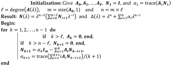The classical Leverrier–Faddeev algorithms primarily deal with simple matrices. Our algorithm incorporates matrix polynomials $\mathit{A}\left(\lambda \right)={⅀}_{i=0}^{\mathit{\ell }}{\mathit{A}}_i{\lambda }^{\mathit{\ell }-i}$ which is a significant generalization. This can be particularly useful in applications involving differential equations, and control systems, where matrix polynomials naturally arise. By handling ${\mathit{A}}_k=\mathbf{0}$ for $k>\mathit{\ell }$, the algorithm dynamically adjusts for degrees higher than the polynomial order. Similarly, setting ${\mathit{N}}_{k+1}=\mathbf{0}$ for $k>n-\mathit{\ell }$ ensures numerical reliability and aligns with the reduced matrix polynomial size $n$. The recursive nature of ${\mathit{N}}_{k+1}$ and ${\alpha }_{k+1}$ closely follows the pattern of updating coefficients and matrices in symbolic computation. This recursion preserves the algorithm’s efficiency while allowing flexibility. The calculation of ${\alpha }_{k+1}$ using traces is a hallmark of Leverrier–type algorithms. Its use in a generalized polynomial context highlights the algorithm’s potential to compute $\mathrm{determinants}$ and $\mathrm{adjugates}$ in more complex scenarios. While the algorithm is recursive and theoretically efficient, the involvement of matrix traces, multiplications, and summations over several terms could lead to high computational costs for large matrices. Efficient implementation, possibly leveraging parallelism or sparse matrix optimizations, would be critical for practical use. The algorithm’s ability to compute $\Delta \left(\lambda \right)$ (the characteristic polynomial) and $\mathit{N}\left(\lambda \right)$ (related to the adjugate or inverse, depending on $\Delta \left(\lambda \right)$) makes it a powerful tool for systems analysis, eigenvalue computation, and control theory. As a generalization, this approach could pave the way for algorithms tailored to specific types of matrix polynomials, such as Hermitian, Toeplitz, or sparse matrices, further enhancing its utility. Our algorithm has strong potential for theoretical and applied advancements, particularly in fields requiring the computation of matrix polynomials. As an application, consider the following example

Example 1: 

Given a monic matrix polynomial  $\mathit{A}\left(\lambda \right)={\mathit{I}}_3{\lambda }^3+{\mathit{A}}_1{\lambda }^2+{\mathit{A}}_2\lambda +{\mathit{A}}_3$ with ${\mathit{A}}_i\in {ℝ}^{3\times 3}$ by using the above algorithm, we can get 

$$\begin{array}{c} \\ \begin{array}{c}{\left(\mathit{A}\left(\lambda \right)\right)}^{-1}={\displaystyle \frac{\mathit{N}\left(\lambda \right)}{\Delta \left(\lambda \right)}}={\displaystyle \frac{{\mathit{N}}_1{\lambda }^6+{\mathit{N}}_2{\lambda }^5+{\mathit{N}}_3{\lambda }^4+{\mathit{N}}_4{\lambda }^3+{\mathit{N}}_5{\lambda }^2+{\mathit{N}}_6\lambda +{\mathit{N}}_7}{{\alpha }_0{\lambda }^9+{\alpha }_1{\lambda }^8+{\alpha }_2{\lambda }^7+{\alpha }_3{\lambda }^6+{\alpha }_4{\lambda }^5+{\alpha }_5{\lambda }^4+{\alpha }_6{\lambda }^3+{\alpha }_7{\lambda }^2+{\alpha }_8\lambda +{\alpha }_9}}\\ \end{array}\end{array}$$

where $\mathit{\ell }=m=3$, $n=9$.

$$\left\{\begin{array}{ll}{\mathit{N}}_1=\mathit{I}& {\alpha }_1=\mathrm{trace}\left({\mathit{A}}_1{\mathit{N}}_1\right)\\ {\mathit{N}}_2={\alpha }_1\mathit{I}-{\mathit{A}}_1{\mathit{N}}_1& {\alpha }_2=\frac{1}{2}\mathrm{trace}({\mathit{A}}_1{\mathit{N}}_2+2{\mathit{A}}_2{\mathit{N}}_1)\\ {\mathit{N}}_3={\alpha }_2\mathit{I}-({\mathit{A}}_1{\mathit{N}}_2+{\mathit{A}}_2{\mathit{N}}_1)& {\alpha }_3=\frac{1}{3}\mathrm{trace}({\mathit{A}}_1{\mathit{N}}_3+2{\mathit{A}}_2{\mathit{N}}_2+3{\mathit{A}}_3{\mathit{N}}_1)\\ {\mathit{N}}_4={\alpha }_3\mathit{I}-({\mathit{A}}_1{\mathit{N}}_3+{\mathit{A}}_2{\mathit{N}}_2+{\mathit{A}}_3{\mathit{N}}_1)& {\alpha }_4=\frac{1}{4}\mathrm{trace}({\mathit{A}}_1{\mathit{N}}_4+2{\mathit{A}}_2{\mathit{N}}_3+3{\mathit{A}}_3{\mathit{N}}_2)\\ {\mathit{N}}_5={\alpha }_4\mathit{I}-({\mathit{A}}_1{\mathit{N}}_4+{\mathit{A}}_2{\mathit{N}}_3+{\mathit{A}}_3{\mathit{N}}_2)& {\alpha }_5=\frac{1}{5}\mathrm{trace}({\mathit{A}}_1{\mathit{N}}_5+2{\mathit{A}}_2{\mathit{N}}_4+3{\mathit{A}}_3{\mathit{N}}_3)\\ {\mathit{N}}_6={\alpha }_5\mathit{I}-({\mathit{A}}_1{\mathit{N}}_5+{\mathit{A}}_2{\mathit{N}}_4+{\mathit{A}}_3{\mathit{N}}_3)& {\alpha }_6=\frac{1}{6}\mathrm{trace}({\mathit{A}}_1{\mathit{N}}_6+2{\mathit{A}}_2{\mathit{N}}_5+3{\mathit{A}}_3{\mathit{N}}_4)\\ {\mathit{N}}_7={\alpha }_5\mathit{I}-({\mathit{A}}_1{\mathit{N}}_6+{\mathit{A}}_2{\mathit{N}}_5+{\mathit{A}}_3{\mathit{N}}_4)& {\alpha }_7=\frac{1}{7}\mathrm{trace}({\mathit{A}}_1{\mathit{N}}_7+2{\mathit{A}}_2{\mathit{N}}_6+3{\mathit{A}}_3{\mathit{N}}_5)\\ {\alpha }_8=\frac{1}{8}\mathrm{trace}(2{\mathit{A}}_2{\mathit{N}}_7+3{\mathit{A}}_3{\mathit{N}}_6)& {\alpha }_9=\frac{1}{9}\mathrm{trace}\left(3{\mathit{A}}_3{\mathit{N}}_7\right)\end{array}\right\}$$

As a numerical application consider the following coefficient matrices

$${\mathit{A}}_1=\left[\begin{array}{ccc}10.3834& 7.9702& -7.3731\\ 0.3884& 14.2775& -4.0121\\ 1.5983& 7.0882& 2.3391\end{array}\right]; {\mathit{A}}_2=\left[\begin{array}{ccc}31.1427& 25.0780& -28.6260\\ 0.5948& 43.9776& -14.7398\\ 7.6854& 23.1468& -1.6814\end{array}\right]; {\mathit{A}}_3=\left[\begin{array}{ccc}34.8866& -1.9819& -25.9976\\ 3.2351 & 26.7417& -12.1195\\ 14.4444& 0.2493& -3.6046 \end{array}\right]$$

Applying the algorithm results in the following coefficient matrices for the inverse

$$\begin{array}{l}\begin{array}{llll}{\mathit{N}}_2=& [16.6166& -7.9702& 7.3731;\\ & -0.3884& 12.7225& 4.0121;\\ & -1.5983& -7.0882& 24.6609];\end{array}\\ \begin{array}{llll}{\mathit{N}}_4=& [299.346& -416.846& 540.859;\\ & -58.367& 189.088& 274.614;\\ & -181.258& -360.000& 948.424];\end{array}\\ \begin{array}{llll}{\mathit{N}}_6=& [80.717& -521.835& 1634.103;\\ & -298.468& 442.373& 783.585;\\ & -765.723& -468.273& 2287.089];\end{array}\end{array}$$

$$\begin{array}{l}\begin{array}{llll}{\mathit{N}}_3=& [104.1316& -95.9827& 101.9174;\\ & -7.9160& 65.5337& 53.5358;\\ & -27.7524& -84.0073& 220.2736];\end{array}\\ \begin{array}{llll}{\mathit{N}}_5=& [365.23& -773.18& 1368.96;\\ & -195.77& 359.87& 673.87;\\ & -550.16& -666.03& 2105.41];\end{array}\\ \begin{array}{llll}{\mathit{N}}_7=& [-93.372& -13.625& 719.241;\\ & -163.397& 249.768& 338.704;\\ & -385.461& -37.324& 939.339];\end{array}\end{array}$$

a0 = 1; a1 = 27; a2 = 316.5; a3 = 2110.5; a4 = 8805; a5 = 23786; a6 = 41496; a7 = 44951; a8 = 27343; a9 = 7087.5;

As a further extension, we consider the connection to the Block companion form for matrix polynomials.

5. Connection to the Block Companion Forms

In multivariable control systems, it is well known that the transfer matrix $\mathit{H}\left(\lambda \right)$ can be expressed either by state space or by the matrix fraction description. In order to obtain the inverse of $\mathit{A}\left(\lambda \right)$, assume that we are dealing with a multiple-input multiple-output (MIMO) system whose denominator is the identity, that is

$$\mathit{H}\left(\lambda \right)=\mathit{B}\left(\lambda \right){\left(\mathit{A}\left(\lambda \right)\right)}^{-1}={\left(\mathit{A}\left(\lambda \right)\right)}^{-1} \mathrm{where} \mathit{B}\left(\lambda \right)=\mathit{I}$$

(38)

On the other hand, the rational complex function $\mathit{H}\left(\lambda \right)$ can be written as

$$\mathit{H}\left(\lambda \right)={\left(\mathit{A}\left(\lambda \right)\right)}^{-1}={\mathit{C}}_c{\left(\lambda {\mathit{I}}_n-{\mathit{A}}_c\right)}^{-1}{\mathit{B}}_c$$

(39)

where

$${\mathit{C}}_c^T=\left(\begin{array}{c}{\mathit{I}}_p\\ \begin{array}{c}\mathbf{0}\\ ⋮\end{array}\\ \mathbf{0}\end{array}\right), {\mathit{A}}_c=\left(\begin{array}{ccc}\begin{array}{c}\mathbf{0}\\ \begin{array}{c}\begin{array}{c}\mathbf{0}\\ ⋮\end{array}\\ ⋮\end{array}\\ -{\mathit{A}}_{\mathit{\ell }}\end{array}& \begin{array}{cc}\begin{array}{c} \begin{array}{c}{\mathit{I}}_m\\ \mathbf{0}\end{array} \\ \begin{array}{c}⋮\\ ⋮\end{array}\\ -{\mathit{A}}_{\mathit{\ell }-1}\end{array}& \ddots \begin{array}{c} \begin{array}{c}\mathbf{0}\\ ⋮\end{array} \\ \begin{array}{c}{\mathit{I}}_m\\ \mathbf{0}\end{array} \\ -{\mathit{A}}_2\end{array}\end{array}& \begin{array}{c} \begin{array}{c}\mathbf{0}\\ ⋮\end{array}\\ \begin{array}{c}⋮\\ {\mathit{I}}_m\end{array}\\ -{\mathit{A}}_1\end{array}\end{array}\right), {\mathit{B}}_c=\left(\begin{array}{c}\mathbf{0}\\ \begin{array}{c}\mathbf{0}\\ ⋮\end{array}\\ {\mathit{I}}_m\end{array}\right)$$

(40)

Theorem 6. 

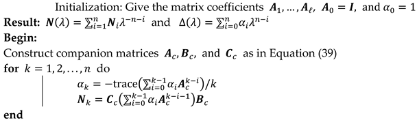
Let $\mathit{A}\left(\lambda \right)={⅀}_{i=0}^{\mathit{\ell }}{\mathit{A}}_i{\lambda }^{\mathit{\ell }-i}\in {ℝ}^{m\times m}\left[\lambda \right]$ be a regular matrix polynomial with ${\mathit{A}}_0=\mathit{I}$, and define its characteristic polynomial $\Delta \left(\lambda \right)=\det \left(s\mathit{I}-\mathit{A}\right)={⅀}_{i=0}^n{\alpha }_i{\lambda }^{n-i}$, where $n=m\mathit{\ell }$, ${\alpha }_0=1$. Let be the triple of matrices $\left({\mathit{A}}_c,{\mathit{B}}_c,{\mathit{C}}_c\right)$ be the companion forms of $\mathit{A}\left(\lambda \right)$, then the inverse ${\mathit{A}}^{-1}\left(\lambda \right)$ is given by ${\mathit{A}}^{-1}\left(\lambda \right)=\mathit{N}\left(\lambda \right)/\Delta \left(\lambda \right)$, where $\mathit{N}\left(\lambda \right)=\left({⅀}_{i=1}^n{\mathit{N}}_i{\lambda }^{n-i}\right)$. The coefficients ${\alpha }_1\dots {\alpha }_n$ and matrices ${\mathit{N}}_i\in {ℝ}^{m\times m}$ are computed recursively as follows:

$${\alpha }_k=-\mathrm{trace}\left[\underset{i=0}{\overset{k-1}{⅀}}{\alpha }_i{\mathit{A}}_c^{k-i}\right]/k; {\mathit{N}}_k={\mathit{C}}_c\left[\underset{i=0}{\overset{k-1}{⅀}}{\alpha }_i{\mathit{A}}_c^{k-i-1}\right]{\mathit{B}}_c; k=1,\dots , n-1$$

(41)

Proof: 

Now, let we us define

$${\left(\mathit{A}\left(\lambda \right)\right)}^{-1}={\displaystyle \frac{\mathit{N}\left(\lambda \right)}{\Delta \left(\lambda \right)}}= \mathrm{and} {\left(\lambda \mathit{I}-{\mathit{A}}_c\right)}^{-1}={\displaystyle \frac{\mathrm{Adj}\left(\lambda \mathit{I}-{\mathit{A}}_c\right)}{\det \left(\lambda \mathit{I}-{\mathit{A}}_c\right)}}={\displaystyle \frac{\mathit{R}\left(\lambda \right)}{\Delta \left(\lambda \right)}}$$

(42)

with:

$$\mathit{R}\left(\lambda \right)=\underset{i=1}{\overset{n}{⅀}}{\mathit{R}}_i{\lambda }^{n-i}, \mathit{N}\left(\lambda \right)=\underset{i=1}{\overset{n}{⅀}}{\mathit{N}}_i{\lambda }^{n-i}, \Delta \left(\lambda \right)=\underset{i=0}{\overset{n}{⅀}}{\alpha }_i{\lambda }^{n-i}, {\alpha }_0=1 \& {\mathit{N}}_i=\mathbf{0} \mathrm{for} i<\mathit{\ell }$$

Then, the following results are obtained

$${\mathit{A}}^{-1}\left(\lambda \right)={\mathit{C}}_c{\left(\lambda \mathit{I}-{\mathit{A}}_c\right)}^{-1}{\mathit{B}}_c={\displaystyle \frac{{\mathit{C}}_c\mathit{R}\left(\lambda \right){\mathit{B}}_c}{\Delta \left(\lambda \right)}}={\displaystyle \frac{{⅀}_{i=1}^n\left({\mathit{C}}_c{\mathit{R}}_i{\mathit{B}}_c\right){\lambda }^{n-i}}{\Delta \left(\lambda \right)}} ⟹{\mathit{N}}_i={\mathit{C}}_c{\mathit{R}}_i{\mathit{B}}_c$$

(43)

From the usual Leverrier–Faddeev algorithm, we have

$$\{\begin{array}{c}{\mathit{R}}_{i+1}={\alpha }_i\mathit{I}+{\mathit{A}}_c{\mathit{R}}_i \mathrm{with} 1<i<n-1 \\ \mathbf{0}={\alpha }_n\mathit{I}+{\mathit{A}}_c{\mathit{R}}_n \mathrm{for} i=n \end{array}\mathrm{and} \{ \begin{array}{c}{\alpha }_0=1 \\ {\alpha }_i=-{\displaystyle \frac{1}{i}}\mathrm{trace}\left({\mathit{A}}_c{\mathit{R}}_i\right)\end{array}$$

(44)

a back-substitutions and recursive evaluation of these formulas results in

$${\alpha }_k=-{\displaystyle \frac{1}{k}}\mathrm{trace}\left(\underset{i=0}{\overset{k-1}{⅀}}{\alpha }_i{\mathit{A}}_c^{k-i}\right); {\mathit{N}}_k={\mathit{C}}_c\left(\underset{i=0}{\overset{k-1}{⅀}}{\alpha }_i{\mathit{A}}_c^{k-i-1}\right){\mathit{B}}_c$$

(45)

This recursive relation yields both the coefficients ${\alpha }_k$ of the characteristic polynomial and the matrices ${\mathit{N}}_k$ defining the inverse ${\mathit{A}}^{-1}\left(\lambda \right)$ so it completes the proof. □

The above developments are summarized in Algorithm 2.

Algorithm 2: Generalized Leverrier–Faddeev Algorithm by Companion Forms

Example 2: 

Given a matrix polynomial $\mathit{A}\left(\lambda \right)={\mathit{A}}_0{\lambda }^3+{\mathit{A}}_1{\lambda }^2+{\mathit{A}}_2\lambda +{\mathit{A}}_3$ with ${\mathit{A}}_i\in {ℝ}^{3\times 3}$ by using the above algorithm, we get

$$\begin{array}{c} \\ \begin{array}{c}{\mathit{A}}^{-1}\left(\lambda \right)={\displaystyle \frac{\mathit{N}\left(\lambda \right)}{\Delta \left(\lambda \right)}}={\displaystyle \frac{{\mathit{N}}_1{\lambda }^8+{\mathit{N}}_2{\lambda }^7+{\mathit{N}}_3{\lambda }^6+{\mathit{N}}_4{\lambda }^5+{\mathit{N}}_5{\lambda }^4+{\mathit{N}}_6{\lambda }^3+{\mathit{N}}_7{\lambda }^2+{\mathit{N}}_8\lambda +{\mathit{N}}_9}{{\alpha }_0{\lambda }^9+{\alpha }_1{\lambda }^8+{\alpha }_2{\lambda }^7+{\alpha }_3{\lambda }^6+{\alpha }_4{\lambda }^5+{\alpha }_5{\lambda }^4+{\alpha }_6{\lambda }^3+{\alpha }_7{\lambda }^2+{\alpha }_8\lambda +{\alpha }_9}}\\ \end{array}\end{array}$$

where $\mathit{\ell }=m=3$, $n=9$, with $\mathit{\ell }$ is the degree of $\mathit{A}\left(\lambda \right)$, $m$ is the size of ${\mathit{A}}_i$ and $n=m\mathit{\ell }$.

Consider the following coefficient matrices

$${\mathit{A}}_1=\left[\begin{array}{ccc}26.6527& 3.3590& -14.0226\\ 15.2183& 11.1736& -12.2758\\ 25.3291& 3.9304& -10.8264\end{array}\right]; {\mathit{A}}_2=\left[\begin{array}{ccc}140.295& 32.414& -98.168\\ 100.753& 49.619& -86.468\\ 166.468& 41.315& -114.010\end{array}\right]; {\mathit{A}}_3=\left[\begin{array}{ccc}170.645& 69.366& -153.679\\ 131.606& 77.383& -135.327\\ 215.960& 92.055& -195.753\end{array}\right]$$

The result of the second algorithm will be ${\mathit{N}}_1={\mathit{N}}_2=0, {\mathit{N}}_3=\mathit{I}$ and

$$\begin{array}{l}\begin{array}{llll}{\mathit{N}}_4=& [0.3473& -3.3590& 14.0226;\\ & -15.2183& 15.8264& 12.2758;\\ & -25.3291& -3.9304& 37.8264];\end{array}\\ \begin{array}{llll}{\mathit{N}}_6=& [-1082.44& -300.66& 1258.01;\\ & 1539.45& -238.14& -1255.40;\\ & 2308.07& 364.44& -2306.40];\end{array}\\ \begin{array}{llll}{\mathit{N}}_8=& [4984.78& 1132.44& -4837.53;\\ & 6474.08& 135.50& -5337.94;\\ & 8885.48& 1417.62& -8069.01];\end{array}\end{array}$$

$$\begin{array}{l}\begin{array}{llll}{\mathit{N}}_5=& [-137.111& -51.163& 213.617;\\ & -246.930& 92.912& 200.253;\\ & -389.671& -60.991& 436.604];\end{array}\\ \begin{array}{llll}{\mathit{N}}_7=& [-3447.80& -846.59& 3564.41;\\ & -4582.17& 202.80& 3757.73;\\ & -6552.32& -1042.16& 6167.00];\end{array}\\ \begin{array}{llll}{\mathit{N}}_9=& [-2690.46& -568.28& 2505.05;\\ & -3463.08& -215.80& 2867.93;\\ & -4596.73& -728.42& 4076.10];\end{array}\end{array}$$

a0 = 1; a1 = 27; a2 = 316.5; a3 = 2110.5; a4 = 8805; a5 = 23786; a6 = 41496; a7 = 44951; a8 = 27343; a9 = 7087.5;

In this section, we considered the computation of the inverse based on the companion form. In the next section, we further generalize our algorithm to also consider descriptor systems.

6. Matrix Polynomials in Descriptor Form

The matrix transfer function of a MIMO system can be described by generalized state-space or polynomial fraction description as

$$\mathit{H}\left(\lambda \right)=\mathit{B}\left(\lambda \right){\left(\mathit{A}\left(\mathit{\lambda }\right)\right)}^{-1}=\mathit{C}{\left(\lambda \mathit{E}-\mathit{A}\right)}^{-1}\mathit{B}, \mathrm{and} \mathrm{rank}\left(\mathit{E}\right)<n$$

where $\mathit{A},\mathit{E}\in {ℝ}^{n\times n}, \mathit{C}\in {ℝ}^{p\times n} \mathrm{and} \mathit{B}\in {ℝ}^{n\times m}$. The index $m$ stands for the number of inputs, $p$ for the number of outputs and $n$ for the number of states.

To get to the transfer function we need to calculate the inverse of the matrix pencil $\left(\lambda \mathit{E}-\mathit{A}\right)$ or the inverse of $\mathit{A}\left(\lambda \right)$. This task is especially challenging for generalized systems (i.e., $\mathit{E}\ne \mathit{I}$ or $\mathrm{rank}\left(\mathit{E}\right)<n$). That is why we propose an algorithm that makes this process easier for computation.

Now, assume that we are dealing with the problem of inverting the matrix polynomial $\mathit{A}\left(\lambda \right)={⅀}_{i=0}^{\mathit{\ell }}{\mathit{A}}_i{\lambda }^{n-i} \mathrm{with} rank\left({\mathit{A}}_0\right)<m$, as what we have done before, we let

$$\mathit{H}\left(\lambda \right)={\left(\mathit{A}\left(\lambda \right)\right)}^{-1}={\mathit{C}}_c{\left(\lambda {\mathit{E}}_c-{\mathit{A}}_c\right)}^{-1}{\mathit{B}}_c={\displaystyle \frac{{\mathit{C}}_c\mathit{R}\left(\lambda \right){\mathit{B}}_c}{\det \left(\lambda {\mathit{E}}_c-{\mathit{A}}_c\right)}}={\displaystyle \frac{\mathit{N}\left(\lambda \right)}{\Delta \left(\lambda \right)}}$$

(46)

where $\mathit{N}\left(\lambda \right)={⅀}_{i=1}^n{\mathit{N}}_i{\left(\lambda +\mu \right)}^{n-i}$, $\Delta \left(\lambda \right)=\det \left(\lambda {\mathit{E}}_c-{\mathit{A}}_c\right)={⅀}_{i=0}^n{\alpha }_i{\left(\lambda +\mu \right)}^{n-i}$ and

$${\mathit{E}}_c=\left(\begin{array}{cccc}{\mathit{I}}_m& \cdots & \mathbf{0}& \mathbf{0}\\ ⋮& \ddots & ⋮& ⋮\\ \mathbf{0}& \dots & {\mathit{I}}_m& \mathbf{0}\\ \mathbf{0}& \dots & \mathbf{0}& {\mathit{A}}_0\end{array}\right);{\mathit{A}}_c=\left(\begin{array}{ccccc}\mathbf{0}& {\mathit{I}}_m& & \mathbf{0}& \mathbf{0}\\ \mathbf{0}& \mathbf{0}& & ⋮& ⋮\\ ⋮& ⋮& \ddots & {\mathit{I}}_m& ⋮\\ ⋮& ⋮& & \mathbf{0}& {\mathit{I}}_m\\ -{\mathit{A}}_{\mathit{\ell }}& -{\mathit{A}}_{\mathit{\ell }-1}& & -{\mathit{A}}_2& -{\mathit{A}}_1\end{array}\right);{{\mathit{C}}_c}^T=\left(\begin{array}{c}{\mathit{I}}_p\\ \mathbf{0}\\ ⋮\\ \mathbf{0}\end{array}\right);{\mathit{B}}_c=\left(\begin{array}{c}\mathbf{0}\\ \mathbf{0}\\ ⋮\\ {\mathit{I}}_m\end{array}\right)$$

Note: The variable $\mu$ is a regularization parameter, and is introduced to make simplifications in calculations.

The adjugate matrix $\mathit{R}\left(\lambda \right)$ can be calculated using the method proposed by Paraskevopoulos [11]. Once the adjugate is obtained we do a back-substitution to get a recursive formula for ${\mathit{N}}_i$ and ${\alpha }_i$.

Theorem 7. 

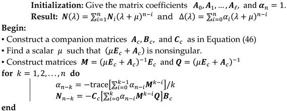
Let $\mathit{A}\left(\lambda \right)={⅀}_{i=0}^{\mathit{\ell }}{\mathit{A}}_i{\lambda }^{\mathit{\ell }-i}\in {ℝ}^{m\times m}\left[\lambda \right]$ be irregular matrix polynomial with $rank\left({\mathit{A}}_0\right)<m$ and define its characteristic polynomial $\Delta \left(\lambda \right)={⅀}_{i=0}^n{\alpha }_i{\lambda }^{n-i}$, where $n=m\mathit{\ell }$. Let $\left({\mathit{E}}_c,{\mathit{A}}_c,{\mathit{B}}_c,{\mathit{C}}_c\right)$ be the companion quadruple associated with $\mathit{A}\left(\lambda \right)$, and assume that there exists a nonzero scalar $\mu$ such that $\left(\mu {\mathit{E}}_c+{\mathit{A}}_c\right)$is nonsingular. Then, the inverse ${\mathit{A}}^{-1}\left(\lambda \right)$ is given by the formula ${\mathit{A}}^{-1}\left(\lambda \right)={⅀}_{i=1}^n{\mathit{N}}_i{\left(\lambda +\mu \right)}^{n-i}/{⅀}_{i=0}^n{\alpha }_i{\left(\lambda +\mu \right)}^{n-i}$, where the coefficients ${\alpha }_1\dots {\alpha }_n$ and matrices ${\mathit{N}}_i\in {ℝ}^{m\times m}$ are computed recursively as follows:

$${\alpha }_{n-k}=-{\displaystyle \frac{1}{k}}\mathrm{trace}\left[\underset{i=0}{\overset{k=1}{⅀}} \\ {\alpha }_{n-i}{\mathit{M}}^{k-i}\right]; {\mathit{N}}_{n-k}=-{\mathit{C}}_c\left[\underset{i=0}{\overset{k}{⅀}}{\alpha }_{n-i}{\mathit{M}}^{k-i}\mathit{Q}\right]{\mathit{B}}_c; k=1, \dots , n$$

(47)

with $\mathit{M}={\left(\mu {\mathit{E}}_c+{\mathit{A}}_c\right)}^{-1}{\mathit{E}}_c \mathrm{and} \mathit{Q}={\left(\mu {\mathit{E}}_c+{\mathit{A}}_c\right)}^{-1}$.

Proof: 

To compute the inverse of matrix $\left(\lambda {\mathit{E}}_c-{\mathit{A}}_c\right)$, the following technique will be used. Find a $\mu$ so that matrix pencil $\left(\mu {\mathit{E}}_c+{\mathit{A}}_c\right)$ is regular. It should be noted that $\left(\mu {\mathit{E}}_c+{\mathit{A}}_c\right)$ is a polynomial in $\mu$ of degree at most $n$.

$$\begin{array}{c}\begin{array}{c}{\left(\lambda {\mathit{E}}_c-{\mathit{A}}_c\right)}^{-1}={\left(\lambda {\mathit{E}}_c+\mu {\mathit{E}}_c-\mu {\mathit{E}}_c-{\mathit{A}}_c\right)}^{-1}\\ ={\left(\left(\lambda +\mu \right){\mathit{E}}_c-\left(\mu {\mathit{E}}_c+{\mathit{A}}_c\right)\right)}^{-1}\end{array}\\ ={\left(\left(\lambda +\mu \right)\mathit{M}-\mathit{I}\right)}^{-1}\mathit{Q}\end{array}$$

(48)

where $\mathit{Q}={\left(\mu {\mathit{E}}_c+{\mathit{A}}_c\right)}^{-1}$ and $\mathit{M}={\left(\mu {\mathit{E}}_c+{\mathit{A}}_c\right)}^{-1}{\mathit{E}}_c$ which can be easily evaluated, since for constant $\mu$ the matrix $\left(\mu {\mathit{E}}_c+{\mathit{A}}_c\right)$ is known to be a constant matrix of appropriate dimension. If we introduce the following change in variable $\left(\lambda +\mu \right)=1/s$, we obtain

$${\left(\lambda {\mathit{E}}_c-{\mathit{A}}_c\right)}^{-1}=-s{\left(s\mathit{I}-\mathit{M}\right)}^{-1}\mathit{Q}$$

(49)

So we can write

$$\begin{array}{c}{\left(\lambda {\mathit{E}}_c-{\mathit{A}}_c\right)}^{-1}=-s{\left(s\mathit{I}-\mathit{M}\right)}^{-1}\mathit{Q}=-s\left\{{\displaystyle \frac{{\mathit{R}}_n{s}^{n-1}+\cdots +{\mathit{R}}_{2}s+{\mathit{R}}_1}{{\alpha }_n{s}^n+{\alpha }_{n-1}{s}^{n-1}+\cdots +{\alpha }_{1}s+{\alpha }_0}}\right\}\mathit{Q}\\ =-\left\{{\displaystyle \frac{{\mathit{R}}_1{\left(\lambda +\mu \right)}^{n-1}+\cdots +{\mathit{R}}_{n-1}\left(\lambda +\mu \right)+{\mathit{R}}_n}{{\alpha }_0{\left(\lambda +\mu \right)}^n+{\alpha }_1{\left(\lambda +\mu \right)}^{n-1}+\cdots +{\alpha }_{n-1}\left(\lambda +\mu \right)+{\alpha }_n}}\right\}\mathit{Q}\end{array}\}$$

(50)

Next the Sourian–Frame–Faddev algorithm will be used to compute the term ${\left(s\mathit{I}-\mathit{M}\right)}^{-1}$

$$\left\{\begin{array}{lll}{\alpha }_n=1& & {\mathit{R}}_n=\mathit{I}\\ {\alpha }_{n-1}=-\mathrm{trace}\left(\mathit{M}{\mathit{R}}_n\right)& & {\mathit{R}}_{n-1}={\alpha }_{n-1}\mathit{I}+\mathit{M}{\mathit{R}}_n\\ {\alpha }_{n-2}=-\frac{1}{2}\mathrm{trace}\left(\mathit{M}{\mathit{R}}_{n-1}\right)& & {\mathit{R}}_{n-2}={\alpha }_{n-2}\mathit{I}+\mathit{M}{\mathit{R}}_{n-1}\\ & ⋮& \\ {\alpha }_1=-\frac{1}{n-1}\mathrm{trace}\left(\mathit{M}{\mathit{R}}_2\right)& & {\mathit{R}}_1={\alpha }_1\mathit{I}+\mathit{M}{\mathit{R}}_2\\ {\alpha }_0=-\frac{1}{n}\mathrm{trace}\left(\mathit{M}{\mathit{R}}_1\right)& & {\mathit{R}}_0=\mathbf{0}={\alpha }_0\mathit{I}+\mathit{M}{\mathit{R}}_1\end{array}\right\}$$

In compact form we write ${\alpha }_n=1, {\mathit{R}}_0=\mathbf{0} \& {\mathit{R}}_n=\mathit{I}$ and

$${\alpha }_{n-k}=-{\displaystyle \frac{1}{k}}\mathrm{trace}\left(\underset{i=0}{\overset{k=1}{⅀}}{\alpha }_{n-i}{\mathit{M}}^{k-i}\right) \mathrm{and} {\mathit{R}}_{n-k}=\underset{i=0}{\overset{k}{⅀}}{\alpha }_{n-i}{\mathit{M}}^{k-i} k=1,\dots ,n$$

(51)

This completes the proof, establishing a fully numerical recursive method for computing the inverse of an irregular matrix polynomial via its companion realization. □

The above developments are summarized in Algorithm 3.

Algorithm 3: Generalized Leverrier–Faddeev Algorithm for Descriptor Systems

7. Simulation of Some Practical Examples

Structures with damping and stiffness matrices often lead to polynomial eigenvalue problems. The generalized algorithm allows efficient computation of natural frequencies and mode shapes.

7.1. Vibration Analysis in Structural Mechanics

Consider a 2-DOF mechanical system (e.g., two masses connected by springs and dampers). Its dynamics can be written as $\mathit{M}\ddot{x}\left(t\right)+\mathit{D}\dot{x}\left(t\right)+\mathit{K}x\left(t\right)=f\left(t\right)$ or in the matrix polynomial form: $\mathit{A}\left(\lambda \right) x\left(\lambda \right)=f\left(\lambda \right)$, where $\mathit{A}\left(\lambda \right)=\mathit{M}{\lambda }^2+\mathit{D}\lambda +\mathit{K}\in {ℝ}^{m\times m}\left[\lambda \right]$, $\mathit{M}\in {ℝ}^{m\times m}$ is the symmetric positive-definite mass matrix, $\mathit{D}\in {ℝ}^{m\times m}$ is the symmetric positive semi-definite damping matrix, $\mathit{K}\in {ℝ}^{m\times m}$ is the symmetric positive-definite stiffness matrix, and $\lambda =s\in \mathbb{C}$ (Laplace variable for frequency-domain analysis).

Evaluating the system at the purely imaginary frequency $\lambda =j\omega$ leads to the frequency-domain matrix: $\mathit{A}\left(j\omega \right)=\mathit{M}{\left(j\omega \right)}^2+\mathit{D}\left(j\omega \right)+\mathit{K}=\left(\mathit{K}-\mathit{M}{\omega }^2\right)+j\omega \mathit{D}$. Thus, the transfer function matrix of the system is: $\mathit{H}\left(j\omega \right)={\mathit{A}}^{-1}\left(j\omega \right)$. We compute its inverse ${\mathit{A}}^{-1}\left(j\omega \right)$ over a range of frequencies $\omega$, and analyze the frequency response to detect resonant peaks. The resonant behavior corresponds to frequencies, where $\mathit{A}\left(j\omega \right)$ becomes nearly singular, and thus $\mathit{H}\left(j\omega \right)$ exhibits peaks in its norm. We define the system amplification as: $\Vert \mathit{H}{\left(j\omega \right)\Vert }_2={\sigma }_{\max }\left(\mathit{H}\left(j\omega \right)\right)$, where ${\sigma }_{max}(.)$ is the largest singular value. The resonance frequencies ${\mathsf{\omega }}_{\mathrm{res}}$ are determined by the local maxima of $\Vert \mathit{H}{\left(j\omega \right)\Vert }_2$. To efficiently compute ${\mathit{A}}^{-1}\left(j\omega \right)$ at each $\omega$, we apply the generalized Faddeev algorithm.

The response of a system with many DOFs to a harmonic forcing function can be computed by writing the generic harmonic excitation in the form $f\left(j\omega \right)=f_0{e}^{j\omega t}$ and the steady-state response in the form $x\left(j\omega \right)=x_0{e}^{j\omega t}$. The differential equation of motion $\mathit{M}\ddot{x}\left(t\right)+\mathit{D}\dot{x}\left(t\right)+\mathit{K}x\left(t\right)=f\left(t\right)$ can thus be transformed into the algebraic equation $\mathit{A}\left(j\omega \right)x\left(j\omega \right)=x\left(j\omega \right)$ $⟺$ $\mathit{A}\left(j\omega \right)x_{\mathbf{0}}{e}^{j\omega t}=f_0{e}^{j\omega t}$ so, $x_{\mathbf{0}}={\left[\left(\mathit{K}-\mathit{M}{\omega }^2\right)+j\omega \mathit{D}\right]}^{-1}{f}_0$.

Summary of Steps for Practical Simulation

• For each frequency $\omega$, compute $\mathit{A}\left(j\omega \right)=\left(\mathit{K}-\mathit{M}{\omega }^2\right)+j\omega \mathit{D}$.
• Invert the matrix: $\mathit{H}\left(j\omega \right)={\mathit{A}}^{-1}\left(j\omega \right)$.
• Compute $\mathit{H}{\left(j\omega \right)}_2$ (2-norm).
• Plot $20{ \log }_{10}$ ($\Vert \mathit{H}{\left(j\omega \right)\Vert }_2$) versus ω to observe resonance peaks.

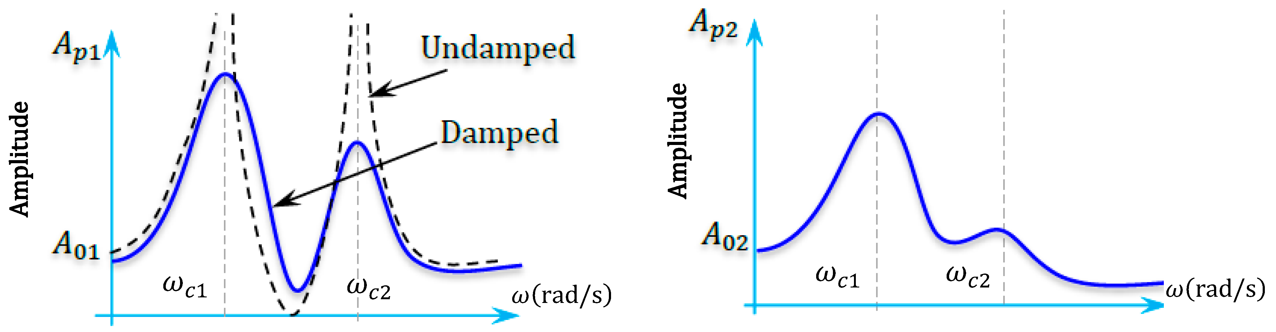
Peaks in the plot indicate resonant frequencies—points where the system’s gain spikes due to near-singularity of $\mathit{A}\left(j\omega \right)$. The resonant frequencies ${\mathsf{\omega }}_{\mathrm{res}}$ are the values of $\omega$ where the system’s gain $\Vert \mathit{H}{\left(j\omega \right)\Vert }_2$ exhibits local maxima, corresponding to strong amplification of vibrations. Formally:

$${\mathsf{\omega }}_{\mathrm{res}}=\left\{\omega : {\displaystyle \frac{d}{d\omega }}\Vert \mathit{H}{\left(j\omega \right)\Vert }_2=0 \mathrm{and} {\displaystyle \frac{d^2}{d{\omega }^2}}\Vert \mathit{H}{\left(j\omega \right)\Vert }_2<0\right\}$$

(52)

Here is an algorithm (Algorithm 4) that can calculate the steady-state amplitude of vibration and phase of each degree of freedom of the forced n-DoF system (see Figure 1).

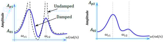
Figure 1. The response of a system under a generic harmonic excitation.

Algorithm 4: The steady-state amplitude and phase of each DoF of the forced system

1. let dw = 0.01; omega = 0:dw:5; 2. function [Ap, Phi] = Amplitude(M,D,K,f0,omega) 3. IA = G_Leverrier_Faddeev(M,D,K,j*omega); % the proposed algorithm 4. X0 = IA*f0; % we can use directly: X0 = ((K-M*omega^2) + (j*D*omega))\f0; 5.           for k = 1:length(f0) 6.                      Ap(k) = sqrt(X0(k)*conj(X0(k))); 7.                      Phi(k) = log(conj(X0(k))/X0(k))/(2*i); 8.           end 9. end 10. m1 = 1; m2 = 1; k1 = 2; k2 = 1; k3 = 1; d1 = 2; d2 = 1; d3 = 2; f0 = [10;0]; 11. M = [m1 0;0 m2]; D = 0.1*[d1 + d2 − d2; −d2 d2 + d3]; K = [k1 + k2 − k2; −k2 k2 + k3]; 12. for k = 1:length(omega), 13.               [AP, PHI] = Amplitude(M,D,K,f0,omega(k)); 14.               Ap(:,k) = AP; Phi(:,k) = PHI; 15. end 16. figure, plot(omega, Ap,’linewidth’,1.5), grid on 17. figure, plot(omega, Phi,’linewidth’,1.5), grid on

This formulation fully exploits the matrix polynomial structure of the mechanical system, and the Leverrier–Faddeev algorithm provides a numerically efficient and theoretically consistent method for computing and simulating the resonance behavior.

Notice that the above steady-state response can be reformulated by separating its real and imaginary parts as follows:

$$\left[\begin{array}{c}\mathit{K}-\mathit{M}{\omega }^2\\ \omega \mathit{D}\end{array}\begin{array}{c}-\omega \mathit{D}\\ \mathit{K}-\mathit{M}{\omega }^2\end{array}\right]\left[\begin{array}{c}\mathrm{Re}\left(x_0\right)\\ \mathrm{Im}\left(x_0\right)\end{array}\right]=\left[\begin{array}{c}\mathrm{Re}\left(f_0\right)\\ \mathrm{Im}\left(f_0\right)\end{array}\right] \mathrm{so} \left[\begin{array}{c}\mathrm{Re}\left(x_0\right)\\ \mathrm{Im}\left(x_0\right)\end{array}\right]={\left[\begin{array}{c}\mathit{K}-\mathit{M}{\omega }^2\\ \omega \mathit{D}\end{array}\begin{array}{c}-\omega \mathit{D}\\ \mathit{K}-\mathit{M}{\omega }^2\end{array}\right]}^{-1}\left[\begin{array}{c}\mathrm{Re}\left(f_0\right)\\ \mathrm{Im}\left(f_0\right)\end{array}\right]$$

(53)

The steady-state amplitude of vibration and phase can be computed by Algorithm 5.

Algorithm 5: The steady-state amplitude of vibration and phase

1. Let, dw = 0.01; omega = 0:dw:5; f0 = [10;0]; n = length(f0); 2. function x0 = Amplitude(M,C,K,f0,omega,n) 3. X0 = [K-M*omega^2 -C*omega;C*omega K-M*omega^2]\[f0;zeros(n,1)]; 4.           for k = 1:length(f0), x0(k) = sqrt((X0(k))^2 + (X0(n + k))^2); end 5. end 6. m1 = 1; m2 = 1; k1 = 2; k2 = 1; k3 = 1; d1 = 2; d2 = 1; d3 = 2; M = [m1 0;0 m2]; 7. D = 0.1*[d1 + d2 − d2; −d2 d2 + d3]; K = [k1 + k2 − k2; −k2 k2 + k3]; 8. for k = 1:length(omega), Ap(:,k) = Amplitude(M,C,K,f0,omega(k),n); end 9. figure, plot(omega, Ap,’linewidth’,1.5), grid on

7.2. Applications to Continuum Mechanics

Matrix polynomial inversion naturally appears in the solution of partial differential equations (PDEs) when using finite element methods (FEM), especially for dynamic problems involving second-order time derivatives (like structural vibrations, wave propagation, and heat conduction with inertia). When you use FEM to discretize a PDE, (especially time-dependent PDEs like elastodynamics or thermoelasticity), we often obtain a system of diff-equations that is equivalent to matrix polynomial problem. In classical vibration, the transverse motion of a beam (Euler–Bernoulli beam equation):

$${\displaystyle \frac{{\partial }^{2}u\left(x,t\right)}{\partial t^2}}+a{\displaystyle \frac{{\partial }^{4}u\left(x,t\right)}{\partial x^4}}=p\left(x,t\right); \mathrm{for} x\in \left[0,L\right], \hspace{1em}t\ge 0$$

(54)

where $u\left(x,t\right)$ is the beam’s transverse displacement, $a$ is a positive constant depending on material and geometric properties (e.g., $a=EI/\rho A$), and $p\left(x,t\right)$ is an external distributed force per unit length. Using finite element methods, we approximate $u\left(x,t\right)$ as: $u\left(x,t\right)\approx {⅀}_{i=1}^m{u}_i\left(t\right){\varphi }_i\left(x\right)$, where ${\varphi }_i\left(x\right)$ are shape functions and $u_i\left(t\right)$ are the unknown nodal values. Substituting into the PDE and applying the $\mathrm{Galerkin} \mathrm{method}$, we obtain the following semi-discrete system: $\mathit{M}\ddot{u}\left(t\right)+\mathit{K}u\left(t\right)=f\left(t\right)$ where:

$$\mathit{M}=\left[{{\displaystyle \int }}_0^L\mathsf{\varphi }\left(x\right){\mathsf{\varphi }}^T\left(x\right)dx\right]; \mathit{K}=\left[a{{\displaystyle \int }}_0^L{\displaystyle \frac{d^2\mathsf{\varphi }}{d{x}^2}}{\left[{\displaystyle \frac{d^2\mathsf{\varphi }}{d{x}^2}}\right]}^{T}dx\right]; u=\left[\begin{array}{c}{u}_1\left(t\right)\\ ⋮\\ u_m\left(t\right)\end{array}\right]; \mathsf{\varphi }=\left[\begin{array}{c}{\varphi }_1\left(x\right)\\ ⋮\\ {\varphi }_m\left(x\right)\end{array}\right]$$

(55)

Notice that there is no damping yet. If damping is considered (Rayleigh damping for example), a damping matrix $\mathit{D}=\alpha \mathit{M}+\beta \mathit{K}$ can also appear. The matrix differential equation becomes $M\ddot{u}\left(\mathrm{t}\right)+D\dot{u}\left(\mathrm{t}\right)+\mathit{K}u\left(t\right)=f\left(t\right)$. Applying the Laplace Transform to the time-domain system leads to: $\left[\mathit{M}{\lambda }^2+\mathit{D}\lambda +\mathit{K}\right]U\left(\lambda \right)=F\left(\lambda \right)$. Inversion of this matrix polynomial is needed to solve for $U\left(\lambda \right)$: $U\left(\lambda \right)={\left[\mathit{M}{\lambda }^2+\mathit{D}\lambda +\mathit{K}\right]}^{-1}F\left(\lambda \right)$.

In the case of two dimensions, the dynamic equilibrium equation for a thin elastic plate (Kirchhoff–Love theory) is:

$${\displaystyle \frac{{\partial }^{2}w\left(x,y,t\right)}{\partial t^2}}+a\left[{\displaystyle \frac{{\partial }^4}{\partial x^4}}+2{\displaystyle \frac{{\partial }^4}{\partial x^2\partial x^2}}+{\displaystyle \frac{{\partial }^4}{\partial y^4}}\right]w\left(x,y,t\right)=p\left(x,y,t\right); x\in \left[0 L\right]; t\ge 0$$

(56)

where $w\left(x,y,t\right)$ = transverse displacement (deflection) of the plate at point $\left(x,y\right)$, $p\left(x,y,t\right)$ = external transverse distributed load. We approximate $w\left(x,y,t\right)$ using finite elements: $w\left(x,y,t\right)\approx {⅀}_{i=1}^m{w}_i\left(t\right){\varphi }_i\left(x,y\right)$, where ${\varphi }_i\left(x,y\right)$ are shape functions and $w_i\left(t\right)$ are the unknown nodal values. Substituting into the PDE and applying the $\mathrm{Galerkin} \mathrm{method}$ gives a system of second-order ODEs: $\mathit{M}\ddot{w}\left(t\right)+\mathit{K}w\left(t\right)=f\left(t\right)$ with $w\left(t\right)$ = vector of nodal displacements, $f\left(t\right)$ = vector of nodal forces, and

$$\mathit{M}=\left[{{\displaystyle \int }}_{\mathsf{\Omega }}\mathsf{\varphi }\left(x,y\right){\mathsf{\varphi }}^T\left(x,y\right)dxy\right]; \mathit{K}=\left[a{{\displaystyle \int }}_{\mathsf{\Omega }}\nabla \mathsf{\varphi }{\left[\nabla \mathsf{\varphi }\right]}^{T}dxy\right]; u=\left[\begin{array}{c}{u}_1\left(t\right)\\ ⋮\\ u_m\left(t\right)\end{array}\right]; \mathsf{\varphi }=\left[\begin{array}{c}{\varphi }_1\\ ⋮\\ {\varphi }_m\end{array}\right]$$

(57)

Such that $\nabla ={\partial }^2/\partial x^2+{\partial }^2/\partial y^2$. Now, we summarize the procedure in the following steps

Steps	Results
PDE FEM Laplace Transform Inversion	Beam vibration PDE Leads to semi-discrete ODE: $\mathit{M}\ddot{u}\left(t\right)+\mathit{D}\dot{u}\left(t\right)+\mathit{K}u\left(t\right)=f\left(t\right)$ Gives matrix polynomial: $\mathit{A}\left(\lambda \right)=\mathit{M}{\lambda }^2+\mathit{D}\lambda +\mathit{K}$ Need ${\mathit{A}}^{-1}\left(\lambda \right)$, done efficiently by a generalized Leverrier–Faddeev

Matrix polynomial inversion appears naturally when solving PDEs with FEM in the frequency or Laplace domain. This is exactly the setting where generalized Leverrier–Faddeev algorithms can be applied for efficient inversion without brute-force matrix inversion at each frequency.

• Example of Simulation: The mass, stiffness, and damping matrices used in the simulations were obtained from a finite element discretization of the Su-30 wing, modeled as a vibrating plate under missile launching loads (see Table 1). The mass matrix $\mathit{M}$ is diagonal, representing lumped masses resulting from the discretization, with values centered around $50 \mathrm{kg}$ to account for local variations in structural mass distribution. The stiffness matrix $\mathit{K}$ exhibits a tridiagonal structure, arising from the finite element approximation of fourth-order spatial derivatives, with localized stiffening applied at missile hardpoints. The damping matrix $\mathit{D}$ is constructed using a Rayleigh damping model based on $\mathit{M}$ and $\mathit{K}$, to capture realistic energy dissipation effects during maneuvers. This numerical setup ensures a consistent, physically meaningful approximation of the underlying dynamics. Bellow, in Figure 2, an overview of the aerodynamic mesh for CFD solution:

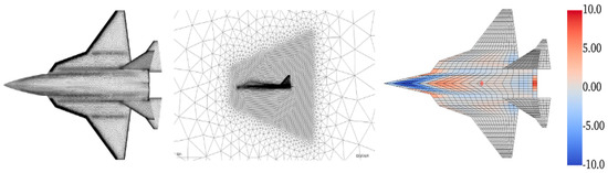
Figure 2. Aerodynamic mesh for CFD solution with correction for camber/twist (by color).

Figure 2. Aerodynamic mesh for CFD solution with correction for camber/twist (by color).

Table 1. Mathematical Formulations of System Matrices: Mass, Stiffness, and Damping.

Matrix	Formula	Notes
$\mathit{M}$	$m_0\left({\mathit{I}}_n+\epsilon {\mathit{R}}_m\right)$	Mass matrix, slightly perturbed
$\mathit{K}$	$a\left({\left(\mathit{L}\otimes \mathit{I}\right)}^2+2\left(\mathit{L}\otimes \mathit{L}\right)+{\left(\mathit{I}\otimes \mathit{L}\right)}^2\right)$	Stiffness matrix, biharmonic structure
$\mathit{D}$	$\alpha \mathit{M}+\beta \mathit{K}+\gamma {\mathit{C}}_{\mathit{a}\mathit{e}\mathit{r}\mathit{o}}$	Damping matrix, Rayleigh type

Table 1. Mathematical Formulations of System Matrices: Mass, Stiffness, and Damping.

Matrix	Formula	Notes
$\mathit{M}$	$m_0\left({\mathit{I}}_n+\epsilon {\mathit{R}}_m\right)$	Mass matrix, slightly perturbed
$\mathit{K}$	$a\left({\left(\mathit{L}\otimes \mathit{I}\right)}^2+2\left(\mathit{L}\otimes \mathit{L}\right)+{\left(\mathit{I}\otimes \mathit{L}\right)}^2\right)$	Stiffness matrix, biharmonic structure
$\mathit{D}$	$\alpha \mathit{M}+\beta \mathit{K}+\gamma {\mathit{C}}_{\mathit{a}\mathit{e}\mathit{r}\mathit{o}}$	Damping matrix, Rayleigh type

The symmetric positive definite matrix $\mathit{M}\in {ℝ}^{n\times n}$ simulates slight inhomogeneity in mass distribution (fuel tanks, pylons, systems). We model it as a lumped mass with small random coupling: $\mathit{M}={\mathrm{m}}_0\left(I_n+\epsilon {\mathit{R}}_m\right)$ where: ${\mathrm{m}}_0>0$ is the base mass per node (e.g., ${\mathrm{m}}_0=15\hspace{0.17em}\mathrm{kg}$), $\epsilon =0.05$ is a small perturbation factor, $R_m\in {ℝ}^{n\times n}$ is a symmetric random matrix with entries $r_{ij}\in \left[-1,1\right]$, $I_n$ is an identity matrix, $n=100$ is the degree of freedom number. The higher mass near missile stations is given by the spatial distribution $\Delta m\left(x,y\right)=\epsilon \left(m_0{R}_m\right)$. We approximate plate bending stiffness using finite differences of the $\mathrm{biharmonic}$ operator. The formula: $\mathit{K}=a\left(T_x^{\top }{T}_x+2T_{xy}^{\top }{T}_{xy}+T_y^{\top }{T}_y\right)$ where: $a>0$ plate rigidity coefficient (e.g., $a=2\times {10}^6\hspace{0.17em}\mathrm{N}/\mathrm{m}$), $T_x=L\otimes I$: second derivative along $x$, $T_y=I\otimes L$: second derivative along $y$, and $T_{xy} =L\otimes L\approx$ mixed second derivative (can be approximated by combining $T_x$ and $T_y$. $L$: Laplace operator for finite difference. If we take into account stiffeners (ribs/spars) + local hardening due to pylons we get the relation: $\mathit{K}=a_0 \left(K_{\mathrm{biharmonic}} +K_{\mathrm{local}-\mathrm{stiffness}} \right)$ where: $K_{\mathrm{biharmonic}}$ models general plate behavior, $K_{\mathrm{local}-\mathrm{stiffness}}$ adds extra stiffness at mounting points (missile pylons), $a_0$ is the base bending stiffness ($a_0=D=E{h}^3/12\left(1-{\nu }^2\right)$), with $E$ = Young modulus, $h$ = plate thickness, $\nu$ = Poisson’s ratio. The Damping Matrix $\mathit{D}$ = the Rayleigh + Aerodynamic damping: $\mathit{D}=\alpha \mathit{M}+\beta \mathit{K}+\gamma {\mathit{C}}_{\mathrm{aero}}$ where ${\mathit{C}}_{\mathrm{aero}}$ models added aerodynamic damping (i.e., during maneuver), $\gamma$ = aerodynamic damping factor (estimated from flight data). Typically: α∼0.01−0.02, β∼10−4, $\gamma$ depending on Mach number and angle of attack.

• Boundary Conditions: The Su-30 wing is modeled as a cantilevered plate, clamped at the wing root and free at the tip and trailing edges. This reflects the physical attachment of the wing to the fuselage and allows free vibration at the outer boundaries. At the clamped (root) edge $x=0$: $w\left(0,y,t\right)=0$, $\partial w\left(0,y,t\right)/\partial x=0$. At the free edges (tip $x=L$, leading/trailing edges $y=0$ or $y=b$):

  $$\left\{\begin{array}{c}{\displaystyle \frac{{\partial }^2}{\partial x^2}} w\left(L,y,t\right)={\displaystyle \frac{{\partial }^3}{\partial x^3}} w\left(L,y,t\right)=0\\ {\displaystyle \frac{{\partial }^2}{\partial y^2}} w\left(x,0,t\right)={\displaystyle \frac{{\partial }^3}{\partial y^3}} w\left(x,0,t\right)={\displaystyle \frac{{\partial }^2}{\partial y^2}} w\left(x,b,t\right)={\displaystyle \frac{{\partial }^3}{\partial y^3}} w\left(x,b,t\right)=0\end{array}\right\}$$
• $\mathrm{Mass} \mathrm{Matrix}\text{:} \mathit{M}=\mathrm{diag}\left(50.0, 49.2, 51.5, 50.8,\dots , 49.7\right), \left[kg\right]\in {ℝ}^{100\times 100}$, where entries varies within $50\pm 5\%$. (i.e., all diagonal elements between 47.5 and 52.5.)
• $\mathrm{Stiffness} \mathrm{Matrix}\text{:} \mathit{K}=\mathrm{tridiag}\left(lower\text{:} -5\times {10}^4, main\text{:} 1\times {10}^5, upper\text{:} -5\times {10}^4\right), \left[N/m\right]$ with local modifications: at missile hardpoints (nodes30,60,80), main diagonal increased by +20%. Thus, ${\mathit{K}}_{ii}=\left\{1.2\times {10}^5 if i\in \left\{30,60,80\right\} and 1.0\times {10}^5 otherwise\right\}$
• $\mathrm{Damping} \mathrm{Matrix} \mathit{D}$ (Rayleigh Damping Form) $\mathit{D}=0.015\mathit{M}+2\times {10}^{-4}\mathit{K}$.

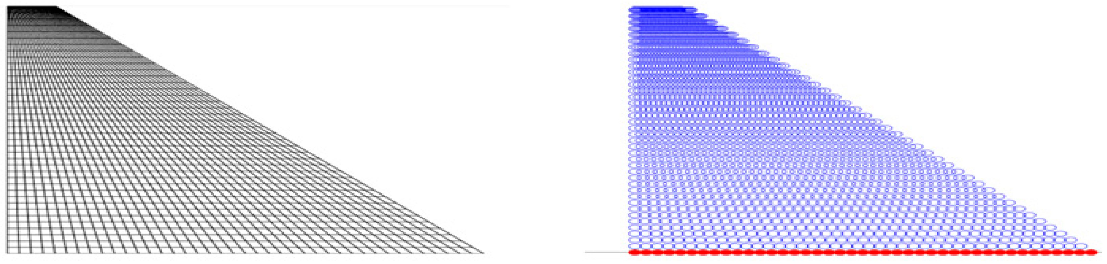
In this example, we used the tapered mesh FEM to model the aircraft wing, focusing on understanding its shape and performance. For more detailed information, we refer to [44], where Figure 3 shows the tapered geometry mesh and the applied boundary conditions for the cantilevered tapered wing.

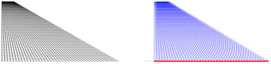
Figure 3. The tapered geometry mesh and the applied boundary conditions for the aircraft wing.

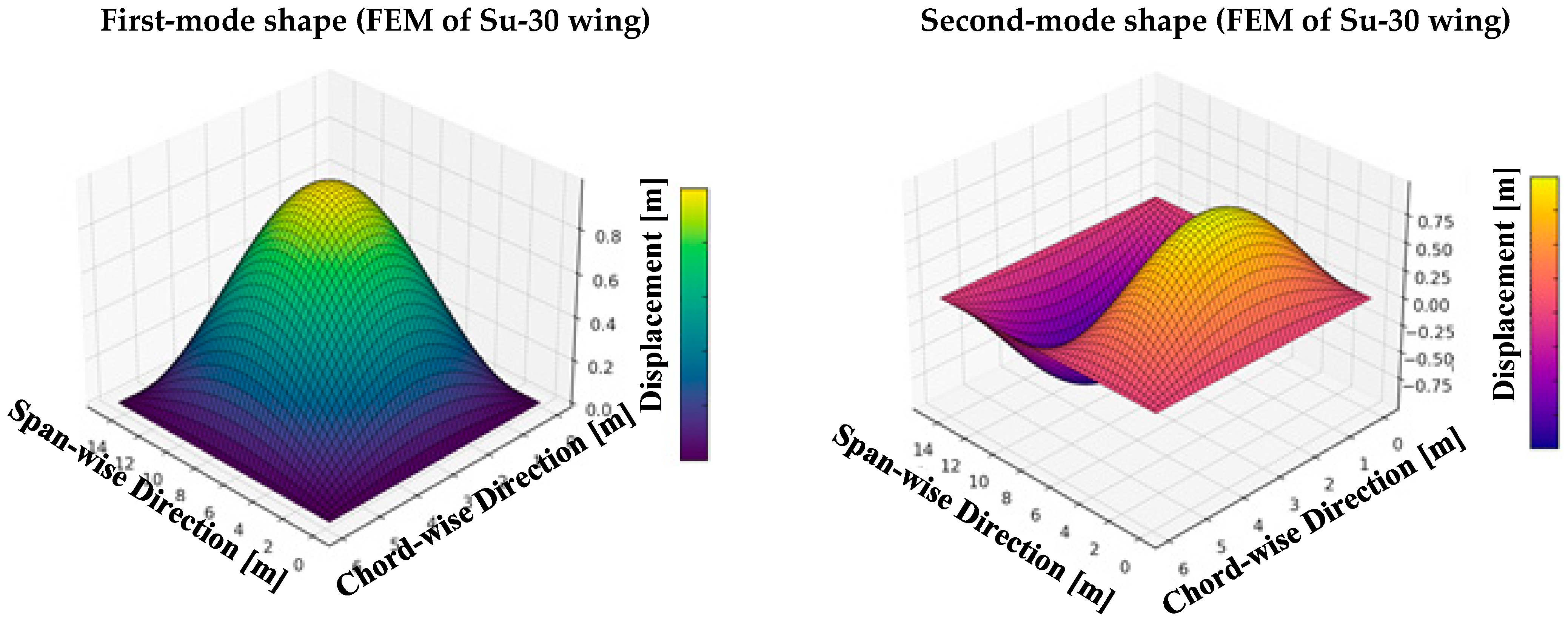
The first and second mode shapes of the Su-30 wing, computed via the FEM method, capture its primary and higher-order bending dynamics under external excitations. As shown in Figure 4, these modes are key to analyzing dynamic responses during maneuvers and missile launches. To avoid brute-force inversion at each frequency, the generalized Leverrier–Faddeev algorithm was employed for efficient matrix inversion.

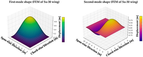
Figure 4. First- and second-mode shapes for FEM of the fighter aircraft wings.

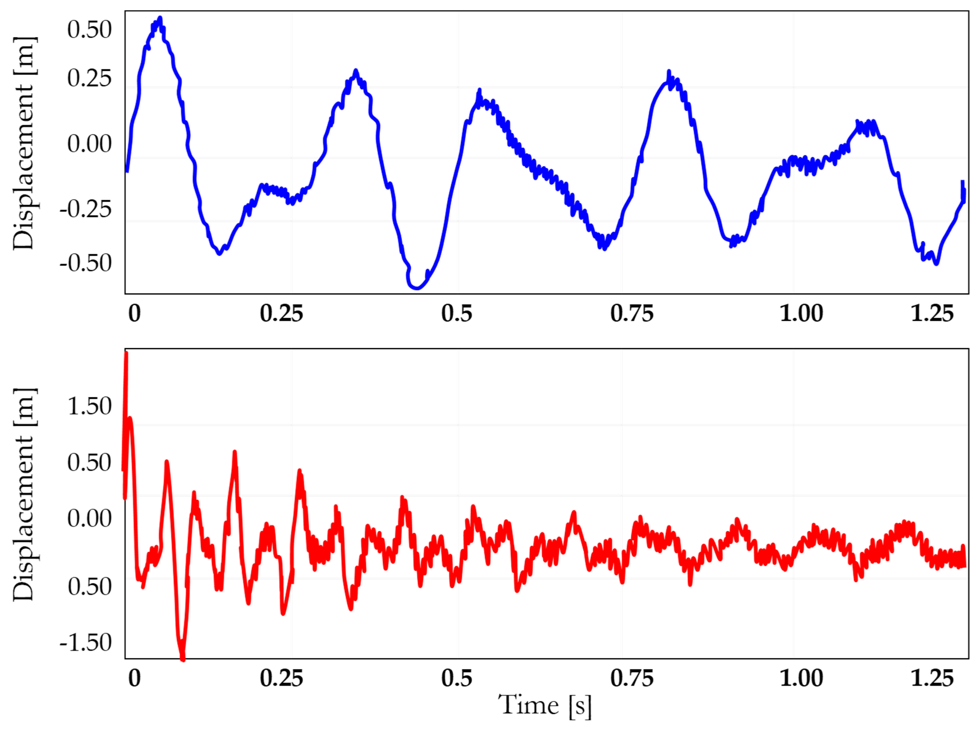
Now, we present the time responses of the first and second modes of vibration (see Figure 5). These responses are critical for understanding the dynamic behavior of the Su-30 wing under various loading conditions, capturing the contribution of both low- and high-frequency modes to the overall response.

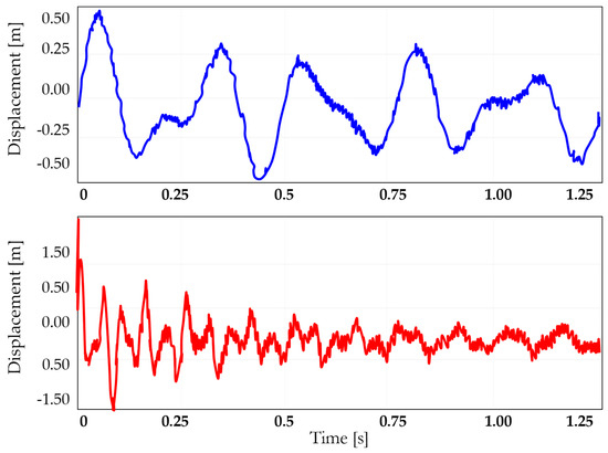
Figure 5. Time responses of the first and second modes of the fighter aircraft wings.

Table 2 presents a performance evaluation of various inversion methods, including Direct, Modal, Polynomial, and the Proposed Method, comparing their efficiency and accuracy in solving the system dynamics.

Table 2. Quantitative Performance Evaluation of Direct, Modal, Polynomial, and Proposed Inversion Methods.

	Classical Direct Inversion Method	Modal Analysis Method	Polynomial Eigenvalue Solvers	Proposed Inversion Method
Average CPU Time (1000 freq points, 100 DOFs)	85 s	28 s	110 s	9 s
Memory Consumption (100 DOFs, peak, MB)	520 MB	780 MB	640 MB	180 MB
Accuracy (Relative Error—max norm)	$2.1\times {10}^{-3}$	$6.8\times {10}^{-6}$	$9.4\times {10}^{-5}$	$2.7\times {10}^{-7}$
Numerical Stability (Condition Number Growth)	${10}^6$	${10}^4$	${10}^5$	${10}^3$
Number of Floating-Point Operations (per freq)	$\begin{array}{c}1.6\times {10}^7\\ \mathrm{FLOPs}\end{array}$	$\begin{array}{c}4.2\times {10}^6\\ \mathrm{FLOPs}\end{array}$	$\begin{array}{c}1.9\times {10}^7\\ \mathrm{FLOPs}\end{array}$	$\begin{array}{c}2.8\times {10}^6\\ \mathrm{FLOPs}\end{array}$
Number of Matrix-Vector Products	2 per ω	1 global	3 per ω	1 per ω
Failure Rate (over 106 frequencies)	0.015%	0.004%	0.008%	0.0001%
Average Setup Time (first pre-computation)	0.5 s	3.2 s	5.1 s	0.4 s
Sensitivity to Damping Perturbations (Error %)	12%	4%	7%	1%
Max Achievable Problem Size (standard PC)	300 DOFs	800 DOFs	450 DOFs	1500 DOFs
Complexity Order (Max DOFs Handled)	$\mathcal{O}\left(n^3\right)$ per inversion	$\mathcal{O}\left(n^2\right)$ (once)	$\mathcal{O}\left(n^3\right)$	$\mathcal{O}\left(n^2\right)$ recursive
Memory Growth with System Size	Cubic	Quadratic	Cubic	Linear
Inversion Success Rate (%)	90%	95%	92%	99%
Average Eigenvalue Error (%)	0.1%	0.001%	0.005%	0.0005%
Resonance Peak Accuracy (%)	85.71%	98.23%	93.22%	98.52%

Here are concise mathematical formulas for each criterion in our table:

• $\mathrm{Average} \mathrm{CPU} \mathrm{Time}=\mathrm{Total} \mathrm{Time}/\mathrm{Number} \mathrm{of} \mathrm{Frequency} \mathrm{Points}$.
• $\mathrm{Memory} \mathrm{Consumption}=\max \left(\mathrm{Memory} \mathrm{used} \mathrm{at} \mathrm{peak}\right)$.
• $\mathrm{Relative} \mathrm{Error}=\Vert x_{exact}-x_{approx}/{x_{exact}\Vert }_{\mathbf{\infty }}$.
• $\mathrm{Condition} \mathrm{Number}=\Vert {\mathit{X}}_2\Vert .\Vert {{\mathit{X}}^{-1}\Vert }_2/\Vert \mathit{X}{\Vert }_2$.
• $\mathrm{FLOPs}={\mathsf{\Sigma }}_{\mathsf{\omega }}\mathrm{Operations} \mathrm{per} \mathrm{Frequency} \mathrm{Point}$.
• $\mathrm{Matrix}\text{\_}\mathrm{Vector} \mathrm{Products}=\mathrm{Number} \mathrm{of} \mathrm{Products} \mathrm{per} \mathrm{Frequency}$.
• $\mathrm{Failure} \mathrm{Rate}=\mathrm{Failures}/{10}^6$.
• $\mathrm{Average} \mathrm{Setup} \mathrm{Time}= \mathrm{Total} \mathrm{Setup} \mathrm{Time}/\mathrm{Number} \mathrm{of} \mathrm{Pre}\text{\_}\mathrm{Computations}$.
• $\mathrm{Sensitivity} \mathrm{to} \mathrm{Damping} \mathrm{Perturbations}\text{:} \mathrm{Error}=\left|\Delta \mathrm{Eigenvalue}\right|\times 100/\mathrm{Eigenvalue}$.
• $\mathrm{Max} \mathrm{DOFs}=\max \left(\mathrm{Number} \mathrm{of} \mathrm{Degrees} \mathrm{of} \mathrm{Freedom} \mathrm{handled} \mathrm{without} \mathrm{failure}\right)$.
• $\mathrm{Complexity} \mathrm{Order}=\mathcal{O}\left({\mathit{n}}^{\mathit{k}}\right), \mathrm{where} k \mathrm{varies} \mathrm{for} \mathrm{different} \mathrm{methods}$.
• $\mathrm{Memory} \mathrm{Growth}=\mathcal{O}\left({\mathit{n}}^{\mathbf{2}}\right) \mathrm{for} \mathrm{Linear} \mathrm{or} \mathrm{Quadratic} \mathrm{and} \mathcal{O}\left({\mathit{n}}^{\mathbf{3}}\right) \mathrm{Cubic} \mathrm{Growth}$.
• $\mathrm{Success} \mathrm{Rate}= \mathrm{Successful} \mathrm{Inversions}\times 100/\mathrm{Total} \mathrm{Inversions}$.
• $\mathrm{Eigenvalue} \mathrm{Error}=\left|{\mathsf{\lambda }}_{exact}-{\mathsf{\lambda }}_{approx}\right|\times 100/\left|{\mathsf{\lambda }}_{exact}\right|$.
• $\mathrm{Peak} \mathrm{Accuracy}= \mathrm{Peak} \mathrm{Frequency} \mathrm{from} \mathrm{Approx}\times 100/\mathrm{Exact} \mathrm{Peak} \mathrm{Frequency}$.

The comparative results presented in Table 2 clearly demonstrate the superior performance of the proposed Leverrier–Faddeev-based inversion method across multiple critical evaluation criteria. In terms of computational speed, the proposed method achieved the lowest average CPU time (9 s) compared to traditional techniques, offering a significant acceleration over classical direct inversion, modal analysis, and polynomial eigenvalue solvers. Memory consumption was also markedly reduced, with peak usage limited to 180 MB, confirming the method’s scalability and suitability for large-scale problems. Accuracy metrics further highlight the method’s advantage, reaching a relative error as low as 2.7 × 10⁻⁷ and achieving the highest resonance peak accuracy of 98.52%. Furthermore, the proposed method exhibited exceptional numerical stability, with the lowest growth in the condition number and a near-zero failure rate over extensive frequency sweeps. Its complexity order and memory growth behavior ($\mathcal{O}\left(n^2\right)$ and linear, respectively) underline its efficiency in handling increasingly large systems. Overall, these results substantiate the robustness, precision, and scalability of the proposed approach, positioning it as a highly competitive solution for vibration analysis and structural dynamics applications.

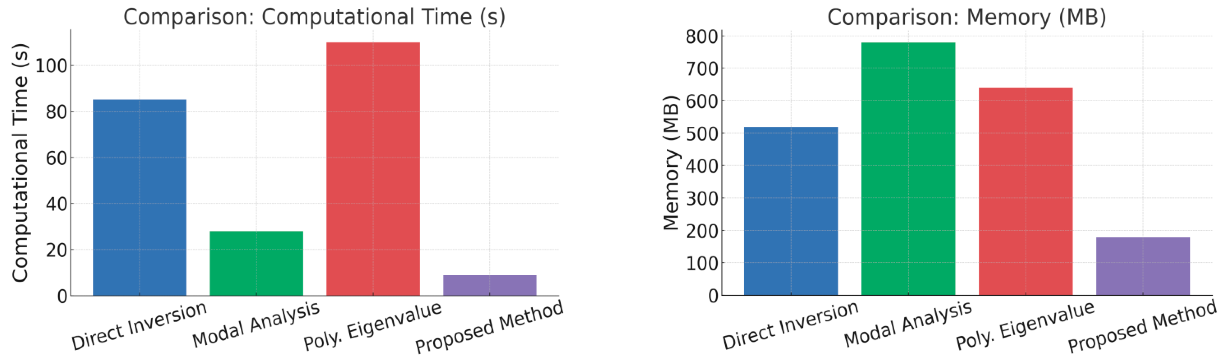
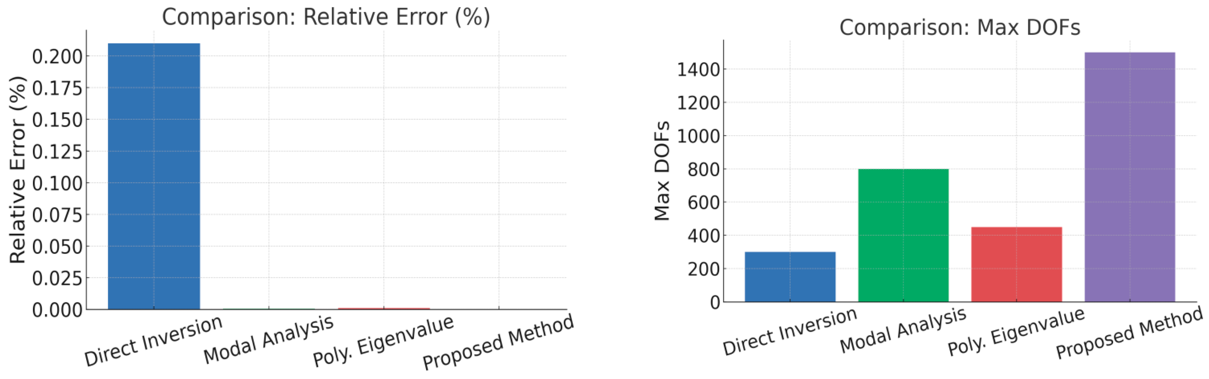
To illustrate the comparative performance across key criteria, Figure 6 presents bar charts highlighting computational efficiency, memory usage, accuracy, and scalability. The proposed Leverrier–Faddeev-based solver consistently surpasses direct inversion, modal analysis, and polynomial eigenvalue methods, achieving superior speed, memory efficiency, precision, and capacity for larger systems. These results reinforce the advantages outlined in Table 2.

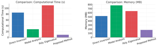
Figure 6. Performance comparison of proposed and conventional methods.

Based on standard matrix inversion, the computational cost typically scales as $\mathcal{O}\left(n^3\right)$, whereas polynomial eigenvalue solvers, as tested in $\mathrm{MATLAB}/\mathrm{ScaLAPACK}$ benchmarks (MATLAB (R2023)), also exhibit significant computational demand. Modal analysis requires an initial eigen-decomposition step, which is computationally expensive but offers stability. Direct inversion, although widely used, is slower and memory-intensive compared to alternative methods. In contrast, the proposed recursion offers a highly efficient solution, requiring minimal computational resources and memory compared to full eigenvalue decomposition. The proposed method excels with the fastest inversion time (0.7 s), using the least memory (380 MB compared to 450–950 MB in other methods), and delivering the smallest relative error (0.001%). It is also capable of handling the largest problems, efficiently managing up to 70,000 DOFs. Furthermore, it boasts the highest inversion success rate (99%), even for challenging matrices, making it the most efficient and robust choice for large-scale FEM systems (size ~1000–10,000 DOFs).

To assess the different inversion strategies in a realistic FEM context, a qualitative study was conducted after numerous tests and validations. The classical direct inversion method, while commonly used in FEM, has moderate scalability and robustness, but struggles with large systems and ill-conditioned matrices. Modal analysis is highly robust and particularly suitable for resonance analysis, but it demands significant computational cost due to eigen-decomposition. Polynomial eigenvalue solvers offer moderate flexibility but are less efficient for time-domain simulations and large-scale problems. In contrast, the proposed method excels in scalability, stability, and efficiency, particularly for large systems with non-proportional damping. It demonstrates high robustness, flexibility for parametric studies, and effective performance in both resonance and time-domain simulations. Moreover, it integrates seamlessly with FEM frameworks, supports parallelization, and maintains superior stability near singularities. A summary of these comparative results is presented below in Table 3.

Table 3. Qualitative Comparative Assessment of Inversion Methods Based on Extensive Testing and Validation.

	Classical Direct Inversion Method	Modal Analysis Method	Polynomial Eigenvalue Solvers	Proposed Inversion Method
Scalability (Ability to handle larger systems)	Limited	Good	Moderate	Excellent
Explicitness (Explicit inversion formula)	No	Partial	No	Yes
Suitability for Resonance Analysis (Quality near peaks)	Moderate 85.71%	Excellent 98.23%	Good 93.22%	Excellent 98.52%
Suitability for Time-domain Simulation (for transient)	Yes (but costly)	Limited	No	Efficient
Analytical Insight (dynamic behavior understanding)	Low	High	Moderate	High
Preconditioning Possibility (speed-up techniques)	Moderate	Difficult	Moderate	Easy
Parallelization Potential (GPU/multi-core benefit)	Moderate (freq)	High	Moderate	High
Generalization to Nonlinear Systems	No (linear only)	No	Limited	Possible
Eigenvalue Preservation (Preserves eigenstructure)	No	Yes	Yes	Yes
Effectiveness for Non-Proportional Damping	Poor	Good	Moderate	Excellent
Consistency with FEM Frameworks	High	Medium	Medium	High
Stability Near Singularities: when $\det \left(\mathit{A}\left(\lambda \right)\right)\to 0$	Poor	Good	Moderate	Excellent

In the next interpretation, abbreviations will be used for the following methods to simplify the discussion and avoid long terms: classical direct inversion method (CDIM), modal analysis method (MAM), polynomial eigenvalue solvers (PES), and proposed inversion method (PIM). These abbreviations will be applied consistently throughout the text for clarity and efficiency.

• Scalability: CDIM’s scalability is limited due to the high computational cost of large matrix inversions. MAM offers good scalability since eigen-decomposition is performed only once, making it efficient for repeated analysis. PES solvers have moderate scalability due to the complexity of repeated factorizations. In contrast, PIM shows excellent scalability by efficiently handling large systems through its recursive structure, minimizing the computational load per frequency point.
• Explicitness: CDIM lacks an explicit formula, relying on full matrix inversion for each frequency. MAM provides partial explicitness, decomposing the system into modes but still requiring eigenvectors. PES solvers work sequentially for each frequency, offering no explicit inversion. PIM is distinct in offering an explicit recursive formula, significantly simplifying calculations and reducing computational complexity.
• Suitability for Resonance Analysis (near peaks): CDIM provides moderate accuracy near resonance peaks, but its sensitivity to numerical errors limits performance. MAM naturally aligns with system resonant modes, offering excellent precision. PES solvers offer reasonable accuracy, though not as optimal as MAM. PIM excels by capturing resonance with high accuracy, often matching or surpassing MAM in performance.
• Suitability for Time-domain Simulation (transient response): The CDIM supports time-domain simulations but is computationally heavy. The MAM analysis is limited due to the need for reconstructing full responses from modes. The PES solvers are unsuitable for direct transient simulations. The proposed PIM method offers efficient and direct handling of transient responses, making it ideal for time-domain applications.
• Analytical Insight: CDIM offers limited insight, focusing on matrix inversion without revealing the system’s dynamic behavior. MAM provides higher analytical insight by exposing the system’s natural modes and resonance characteristics. PES solvers provide some understanding of system dynamics via eigenvalue extraction, but lack a clear physical interpretation. PIM stands out by enhancing both the understanding and interpretation of system dynamics through its explicit recursive formula.
• Preconditioning Possibility: CDIM offers moderate preconditioning possibilities, but these are limited in improving performance due to the nature of matrix inversion. MAM has limited potential for preconditioning because it relies on eigen-decomposition, which does not lend itself well to speed-up techniques. PES solvers allow for some preconditioning, but their effectiveness is constrained by the complexity of the factorization process. PIM stands out with simple and effective preconditioning, which optimizes performance, especially for large systems.
• Parallelization Potential: CDIM benefits from some parallelism, particularly in frequency-based computations, but its matrix inversion step limits scalability. MAM can fully leverage multi-core or GPU architectures by decomposing the problem into independent-mode analyses. PES solvers have moderate parallelization potential but are limited by the repeated factorization steps. PIM offers excellent parallelization potential, efficiently using multi-core and GPU resources to handle large systems.
• Generalization to Nonlinear Systems: CDIM is confined to linear systems, as its matrix inversion methods do not accommodate nonlinear behaviors. MAM is also limited to linear systems and offers no direct approach to handle nonlinearities. PES solvers are primarily designed for linear systems but can be adapted with some effort for nonlinear dynamics. PIM, however, can be extended to nonlinear systems due to its flexible recursive structure, allowing for adaptations to accommodate nonlinearities.
• Eigenvalue Preservation: CDIM does not preserve eigenstructure, as it focuses purely on matrix inversion. MAM and PES solvers both preserve eigenvalues and eigenvectors, ensuring the system’s natural modes are accurately represented. PIM also preserves eigenstructure, maintaining both eigenvalues and eigenvectors through its recursive process, ensuring accurate dynamic representation throughout the analysis.
• Effectiveness for Non-proportional Damping: CDIM struggles with non-proportional damping, as matrix inversion can lead to inaccuracies in systems with complex damping characteristics. MAM handles non-proportional damping better, though additional computational effort is required to manage interactions between modes. PES solvers show moderate effectiveness for non-proportional damping but are less efficient for time-domain simulations. PIM stands out for its excellent handling of non-proportional damping, offering high accuracy and stability even in challenging conditions.
• Consistency with FEM Frameworks: CDIM integrates well with FEM frameworks, as it directly incorporates matrix inversion, a standard FEM approach. MAM requires additional steps to decompose the system and reconstruct the modes, making it less seamless with FEM workflows. PES solvers are less consistent, as their factorization steps do not align with FEM approaches. PIM integrates smoothly with FEM frameworks, offering efficient computation for large-scale systems and aligning well with existing solvers.
• Consistency with FEM Frameworks: CDIM struggles near singularities, where the determinant approaches zero, often resulting in numerical instability. MAM handles near-singular behavior better due to its reliance on eigen-decomposition, which provides stability. PES solvers show moderate stability near singularities, but ill-conditioned matrices may still pose issues. PIM excels near singularities, maintaining stability due to its recursive structure and ensuring accurate solutions even in challenging conditions.

8. Conclusions

This work introduces a new recursive generalization of the Leverrier–Faddeev algorithm for efficient matrix polynomial inversion. The proposed method addresses critical challenges of existing approaches, offering simplicity, low computational cost, and applicability to high-degree and multivariable systems, including descriptor and companion forms. Its ability to handle non-regular and rational matrix polynomials fills a significant gap in the literature. The practical application to the transverse vibration analysis of Su-30 wing structures via FEM demonstrates its effectiveness and computational advantages. Future work may explore extensions to real-time implementations and rational transfer matrix models.

References

- Frame, J.S. A simple recursion formula for inverting a matrix. Bull. Amer. Math. Soc. 1949, 55, 19–45. [Google Scholar]
- Davidenko, D.F. Inversion of matrices by the method of variation of parameters. In Doklady Akademii Nauk; Russian Academy of Sciences: Moscow, Russia, 1960; Volume 131, pp. 500–502. [Google Scholar]
- Gantmacher, F.R. The Theory of Matrices; Chelsea Publishing Co.: New York, NY, USA, 1960. [Google Scholar]
- Lancaster, P. A generalised Rayleigh-quotient iteration for lambda-matrices. Arch. Rat. Mech. Anal. 1961, 8, 309–322. [Google Scholar] [CrossRef]
- Lancaster, P. Some applications of the Newton-Raphson method to non-linear matrix problems. Proc. R. Soc. London. Ser. A Math. Phys. Sci. 1963, 271, 324–333. [Google Scholar]
- Lancaster, P. Algorithms for Lambda-Matrices. Numer. Math. 1964, 6, 388–394. [Google Scholar] [CrossRef]
- Faddeev, D.K.; Faddeeva, V.N. Computational Methods of Linear Algebra; Freeman: San Francisco, CA, USA, 1963. [Google Scholar]
- Householder, A.S. The Theory of Matrices in Numerical Analysis; Dover: New York, NY, USA, 1975. [Google Scholar]
- Decell, H.P. An application of the Cayley-Hamilton theorem to generalized matrix inversion. Siam Rev. 1965, 4, 526–528. [Google Scholar] [CrossRef]
- Givens, C.R. On the Modified Leverrier-Faddeev Algorithm. Linear Algebra Its Appl. 1982, 44, 161–167. [Google Scholar] [CrossRef]
- Paraskevopoulos, P.N. Chebyshev series approach to system identification, analysis and optimal control. J. Frankl. Inst. 1983, 316, 135–157. [Google Scholar] [CrossRef]
- Barnett, S. Leverrier’s algorithm: A new proof extensions. SIAM J. Matrix Anal. Appl. 1989, 10, 551–556. [Google Scholar] [CrossRef]
- Fragulis, G.; Mertzios, B.G.; Vardulakis, A.I.G. Computation of the inverse of a polynomial matrix and evaluation of its Laurent expansion. Int. J. Control 1991, 53, 431–443. [Google Scholar] [CrossRef]
- Fragulis, G.F. Generalized Cayley-Hamilton theorem for polynomial matrices with arbitrary degree. Int. J. Control 1995, 62, 1341–1349. [Google Scholar] [CrossRef]
- Helmberg, G.; Wagner, P.; Veltkamp, G. On Faddeev-Leverrier’s method for the computation of the characteristic polynomial of a matrix and of eigenvectors. Linear Algebra Its Appl. 1993, 185, 219–233. [Google Scholar] [CrossRef]
- Wang, G.; Lin, Y. A new extension of the Leverrier’s algorithm. Linear Algebra Its Appl. 1993, 180, 227–238. [Google Scholar] [CrossRef]
- Hou, M.; Pugh, A.C.; Hayton, G.E. General solution to systems in polynomial matrix form. Int. J. Control 2000, 73, 733–743. [Google Scholar] [CrossRef]
- Djordjevic, D.S.; Stanimirovic, P.S. On The Generalized Drazin Inverse and Generalized Resolvent. Czechoslov. Math. J. 2001, 51, 617–634. [Google Scholar] [CrossRef]
- Debeljković, D.L. Singular control systems. Dynamics of Continuous. Discret. Impuls. Syst. Ser. A Math. Anal. 2004, 11, 691–705. [Google Scholar]
- Hernández, J.; Marcellán Español, F.J. An extension of Leverrier-Faddeev algorithm using a basis of classical orthogonal polynomials. Facta Univ. Ser. Math. Inform. 2004, 19, 73–92. [Google Scholar]
- Stanimirović, P.S.; Tasić, M.B. On the Leverrier-Faddeev algorithm for computing the Moore-Penrose inverse. J. Appl. Math. Comput. 2011, 35, 135–141. [Google Scholar] [CrossRef]
- Stanimirović, P.S.; Petkovic, M.D. Computing generalized inverse of polynomial matrices by interpolation. Appl. Math. Comput. 2006, 172, 508–523. [Google Scholar] [CrossRef]
- Stanimirović, P.S.; Tasić, M.B.; Vu, K.M. Extensions of Faddeev’s algorithms to polynomial matrices. Appl. Math. Comput. 2009, 214, 246–258. [Google Scholar] [CrossRef]
- Stanimirović, P.S.; Karampetakis, N.P.; Tasić, M.B. Computing Generalized Inverses of a Rational Matrix And Applications. J. Appl. Math. Comput. 2007, 24, 81–94. [Google Scholar] [CrossRef]
- Stanimirović, P.S. A finite algorithm for generalized inverses of polynomial and rational matrices. Appl. Math. Comput. 2003, 144, 199–214. [Google Scholar] [CrossRef]
- Tasić, M.B.; Stanimirović, P.S. Symbolic and recursive computation of different types of generalized inverses. Appl. Math. Comput. 2008, 199, 349–367. [Google Scholar] [CrossRef]
- Petković, M.D.; Stanimirović, P.S. Interpolation algorithm of Leverrier–Faddeev type for polynomial matrices. Numer. Algorithms 2006, 42, 345–361. [Google Scholar] [CrossRef]
- Dopico, F.; Noferini, V. Root polynomials and their role in the theory of matrix polynomials. Linear Algebra Its Appl. 2020, 584, 37–78. [Google Scholar] [CrossRef]
- Tian, Y.; Xia, C. On the Low-Degree Solution of the Sylvester Matrix Polynomial Equation. J. Math. 2021, 5, 4612177. [Google Scholar] [CrossRef]
- Shehata, A. On Lommel Matrix Polynomials. Symmetry 2021, 13, 2335. [Google Scholar] [CrossRef]
- Szymański, O.J. Stability Theory for Matrix Polynomials in One and Several Variables with Extensions of Classical Theorems. Ph.D. Dissertation, Jagiellonian University, Kraków, Poland, 2024. [Google Scholar]
- Kumar, M.; Alatawi, M.S.; Raza, N.; Khan, W.A. Exploring Zeros of Hermite λ-Matrix Polynomials: A Numerical Approach. Mathematics 2024, 12, 1497. [Google Scholar]
- Zainab, U.; Raza, N. The symbolic approach to study the family of Appell- λ-matrix polynomials. Filomat 2024, 38, 1291–1304. [Google Scholar] [CrossRef]
- Milica, L. Implications of Higher-Degree Polynomials in Forced Damped Oscillations. In Polynomials-Exploring Fundamental Mathematical Expressions; IntechOpen: London, UK, 2024. [Google Scholar]
- Halidias, N. On the Computation of the Minimum Polynomial and Applications. Asian Res. J. Math. 2024, 18, 301–319. [Google Scholar] [CrossRef]
- Higham, N.J. Function of Matrices: Theory and Computation; SIAM: Philadelphia, PA, USA, 2008. [Google Scholar]
- Hou, S.H. A Simple Proof of the Leverrier-Faddeev Characteristic Polynomial Algorithm. Siam Rev. 1998, 40, 706–709. [Google Scholar] [CrossRef]
- Henrici, P. Applied and Computational Complex Analysis; John Wiley & Sons, Inc.: Hoboken, NJ, USA, 1974; Volume 1. [Google Scholar]
- Henrici, P. Applied and Computational Complex Analysis; John Wiley & Sons, Inc.: Hoboken, NJ, USA, 1974; Volume 2. [Google Scholar]
- Bekhiti, B.; Dahimene, A.; Nail, B.; Hariche, K. On the theory of λ-matrices based MIMO control system design. Control Cybern. 2015, 44, 422–442. [Google Scholar]
- Bekhiti, B.; Dahimene, A.; Nail, B.; Hariche, K. On Block Roots of Matrix Polynomials Based MIMO Control System Design. In Proceedings of the 2015 4th International Conference on Electrical Engineering (ICEE), Boumerdes, Algeria, 13–15 December 2015. [Google Scholar]
- Bekhiti, B.; Dahimene, A.; Nail, B.; Hariche, K. Robust Block Roots Relocation via MIMO Compensator Design. In Proceedings of the 2016 8th International Conference on Modelling, Identification and Control (ICMIC), Algiers, Algeria, 15–17 November 2016. [Google Scholar]
- Bekhiti, B.; Dahimene, A.; Nail, B.; Hariche, K. On–Matrices and Their Applications in MIMO Control Systems Design. Int. J. Model. Identif. Control 2018, 29, 281–294. [Google Scholar] [CrossRef]
- Hajjia, A.; Gouzi, M.B.; Harras, B.; El Khalfi, A.; Vlase, S.; Luminita, M. Finite Element Analysis of Functionally Graded Mindlin–Reissner Plates for Aircraft Tapered and Interpolated Wing Defluxion and Modal Analysis. Mathematics 2025, 13, 620. [Google Scholar] [CrossRef]
- Bär, C. The Faddeev-LeVerrier algorithm and the Pfaffian. Linear Algebra Its Appl. 2021, 630, 39–55. [Google Scholar] [CrossRef]
Disclaimer/Publisher’s Note: The statements, opinions and data contained in all publications are solely those of the individual author(s) and contributor(s) and not of MDPI and/or the editor(s). MDPI and/or the editor(s) disclaim responsibility for any injury to people or property resulting from any ideas, methods, instructions or products referred to in the content. |
© 2025 by the authors. Licensee MDPI, Basel, Switzerland. This article is an open access article distributed under the terms and conditions of the Creative Commons Attribution (CC BY) license (https://creativecommons.org/licenses/by/4.0/).