Author Contributions
Conceptualization, M.R.E.; Methodology, J.H.O. and A.A.H.; Software, J.H.O.; Validation, J.H.O.; Formal analysis, J.H.O.; Investigation, J.H.O.; Resources, J.H.O.; Data curation, J.H.O.; Writing—original draft, J.H.O.; Writing—review & editing, J.H.O., A.A.H. and K.L.W.; Visualization, J.H.O.; Supervision, A.A.H., M.R.E. and K.L.W.; Project administration, A.A.H. and M.R.E.; Funding acquisition, M.R.E. All authors have read and agreed to the published version of the manuscript.
Figure 1.
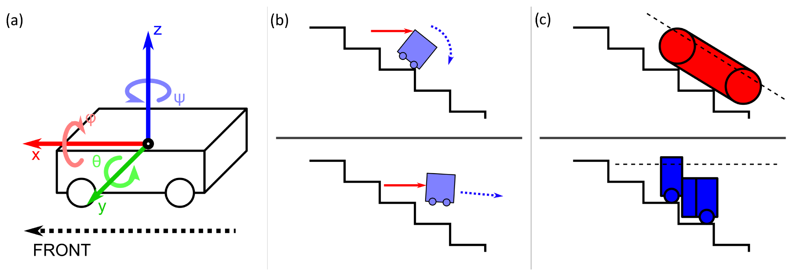
(a) Axes of reference on a robot for discussions in this work. Forces along the x-axis are represented in red and torque about the x-axis is represented in pink, forces along the y-axis are represented in green and torque about the y-axis is represented in light green, and forces along the z-axis are represented in blue and torque about the z-axis is represented in light blue. (b) The two extreme possible ways for a robot to fall off stairs, in real-world scenarios, falls tend to be in between these two extremes. (c) Two general types of stair-climbing robots: those that align with the gradient of the steps and those that remain parallel to the ground when climbing.
Figure 1.
(a) Axes of reference on a robot for discussions in this work. Forces along the x-axis are represented in red and torque about the x-axis is represented in pink, forces along the y-axis are represented in green and torque about the y-axis is represented in light green, and forces along the z-axis are represented in blue and torque about the z-axis is represented in light blue. (b) The two extreme possible ways for a robot to fall off stairs, in real-world scenarios, falls tend to be in between these two extremes. (c) Two general types of stair-climbing robots: those that align with the gradient of the steps and those that remain parallel to the ground when climbing.
Figure 2.
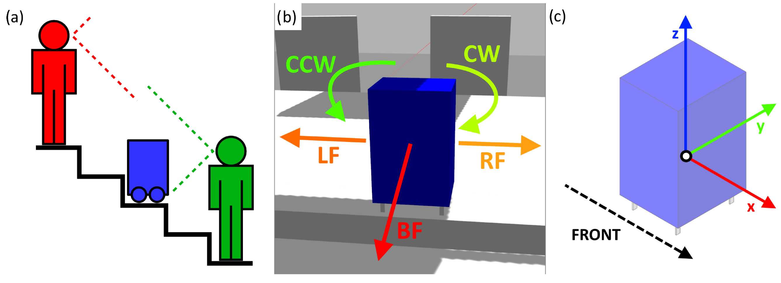
(a) Field of view of people on staircases with the robot. (b) The possible fall types identified. (c) Axes of reference of the virtual model and prototype. The origin is at the geometrical center of the main body of the model (blue).
Figure 2.
(a) Field of view of people on staircases with the robot. (b) The possible fall types identified. (c) Axes of reference of the virtual model and prototype. The origin is at the geometrical center of the main body of the model (blue).
Figure 3.
(a) Setup for the physical data collection. (b) Camera view from cameras mounted at different angles.
Figure 3.
(a) Setup for the physical data collection. (b) Camera view from cameras mounted at different angles.
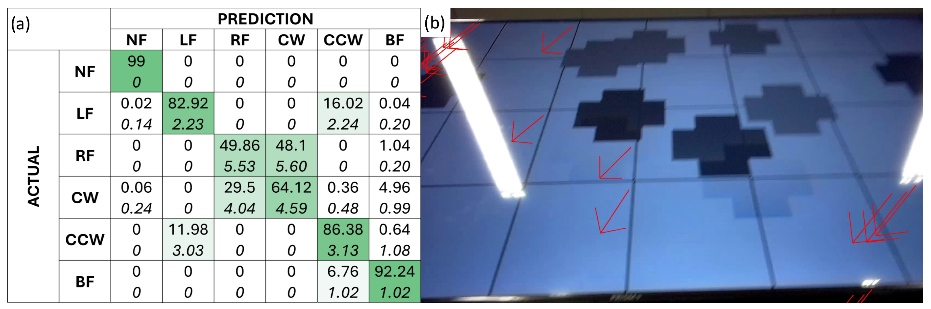
Figure 7.
(a) Confusion matrix depicting the prediction outcomes of 50 LSTM models on the real-world dataset. The mean prediction is given at the top of each cell, and the standard deviation of the outcomes is given in italics below. The cells are shaded based on the mean prediction, with a darker green for a higher mean. (b) Frames from the simulation with the optical flow vectors represented by red arrows visualized for the LF, RF, CCW, and CW classes. An illustration of the general optical vector flow for each fall class is given in green dashed arrows, while the actual optical flow vectors for each frame are shown in red arrows.
Figure 8.
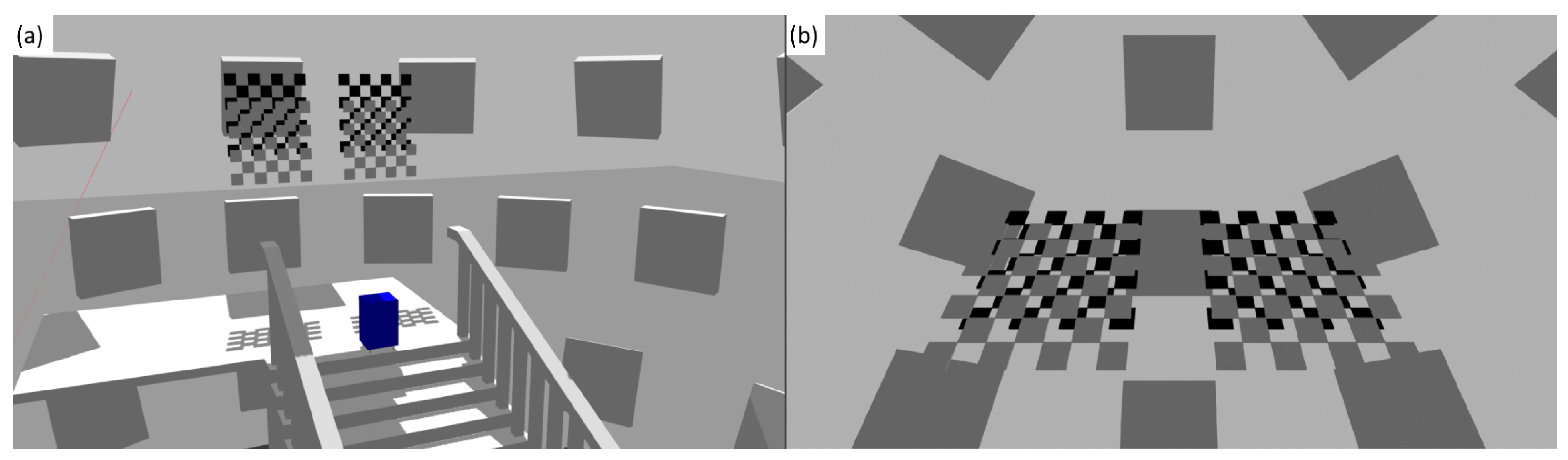
(a) Simulated dynamic environment used for data generation. (b) View from the camera.
Figure 8.
(a) Simulated dynamic environment used for data generation. (b) View from the camera.
Figure 9.
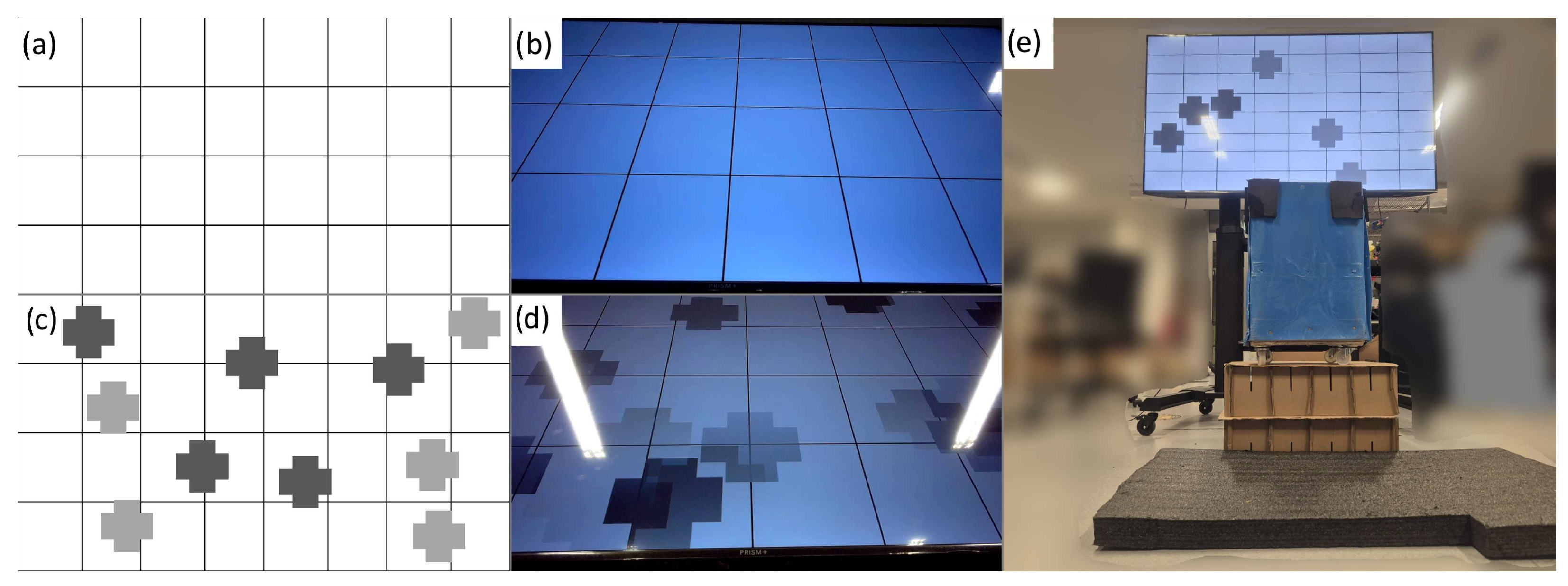
(a) Screenshot from the control video. (b) Camera view when testing with the control video. (c) Screenshot from video with moving features; the grey crosses move across the screen randomly during testing. (d) Camera view when testing the video with moving features. (e) Picture of the data collection setup.
Figure 9.
(a) Screenshot from the control video. (b) Camera view when testing with the control video. (c) Screenshot from video with moving features; the grey crosses move across the screen randomly during testing. (d) Camera view when testing the video with moving features. (e) Picture of the data collection setup.
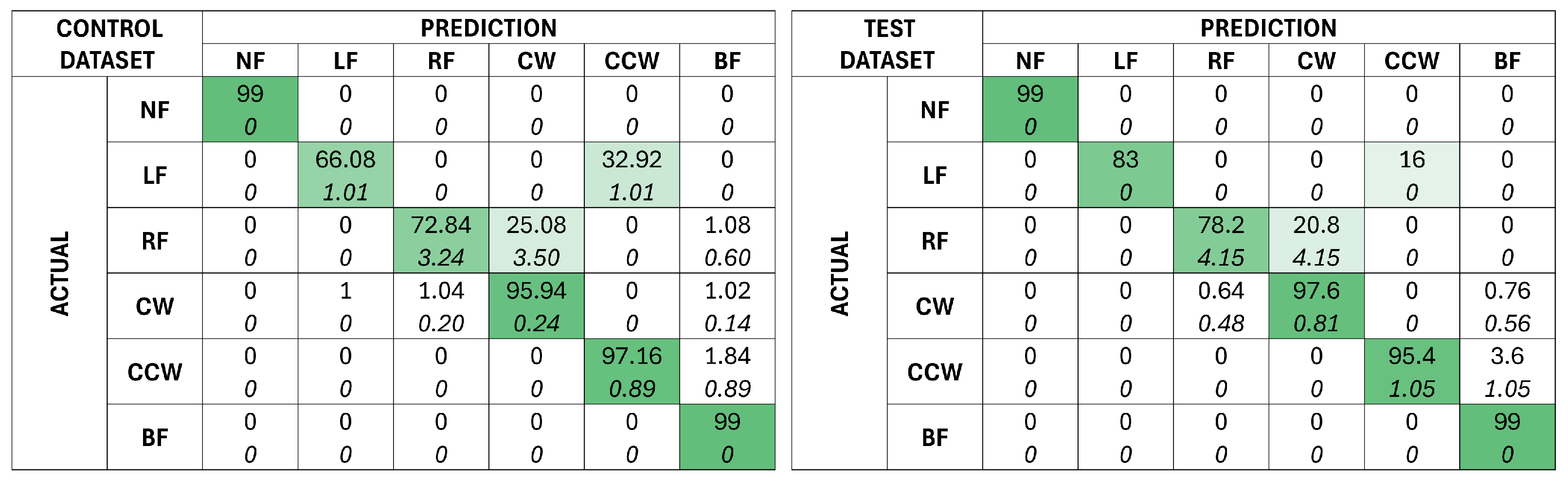
Figure 10.
Confusionmatrices depicting the prediction outcomes of 50 control models on the control (left) and test (right) dataset. The mean prediction is given at the top of each cell, and the standard deviation of the outcomes is given in italics below. The cells are shaded based on the mean prediction, with a darker green for a higher mean.
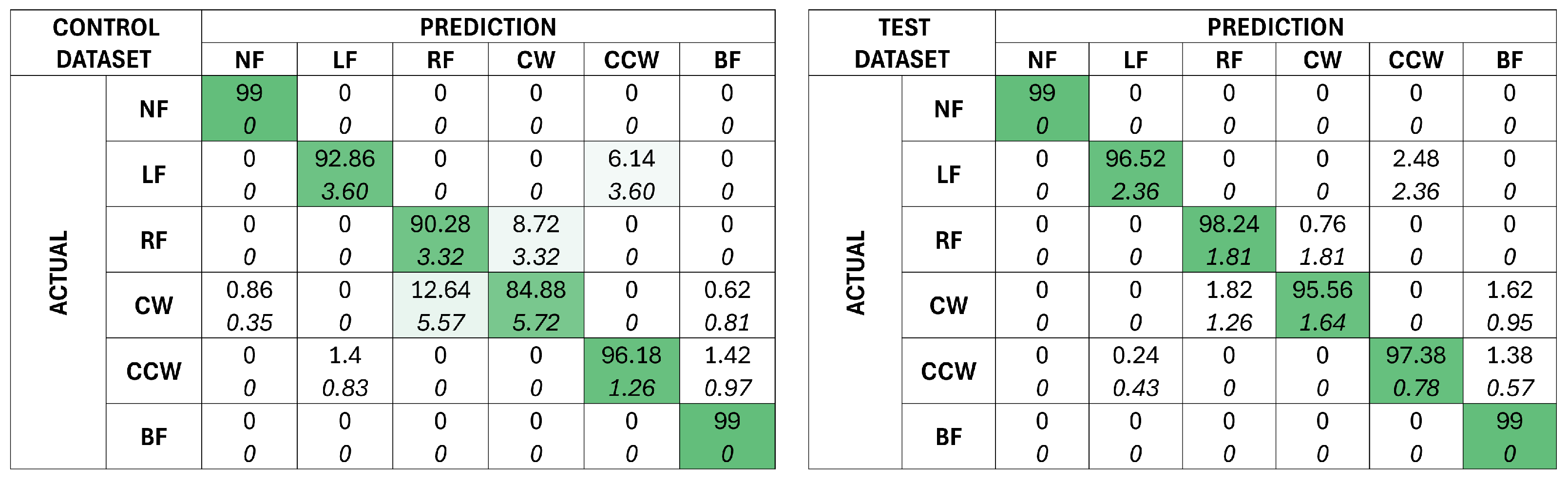
Figure 11.
Confusion matrices depicting the prediction outcomes of 50 test models on the control (left) and test (right) dataset. The mean prediction is given at the top of each cell, and the standard deviation of the outcomes are given in italics below. The cells are shaded based on the mean prediction, with a darker green for a higher mean.
Figure 12.
(a) Confusion matrix depicting the prediction outcomes of 50 test models on the real-world dataset. The mean prediction is given at the top of each cell, and the standard deviation of the outcomes is given in italics below. The cells are shaded based on the mean prediction, with a darker green for a higher mean. (b) A frame from a test with dynamic visual features with the optical flow vectors visualized, the start of the arrows indicating the initial location of the features, the direction being the movement of the visual features, and the length being the magnitude of the movement, magnified 10x for better visual clarity.
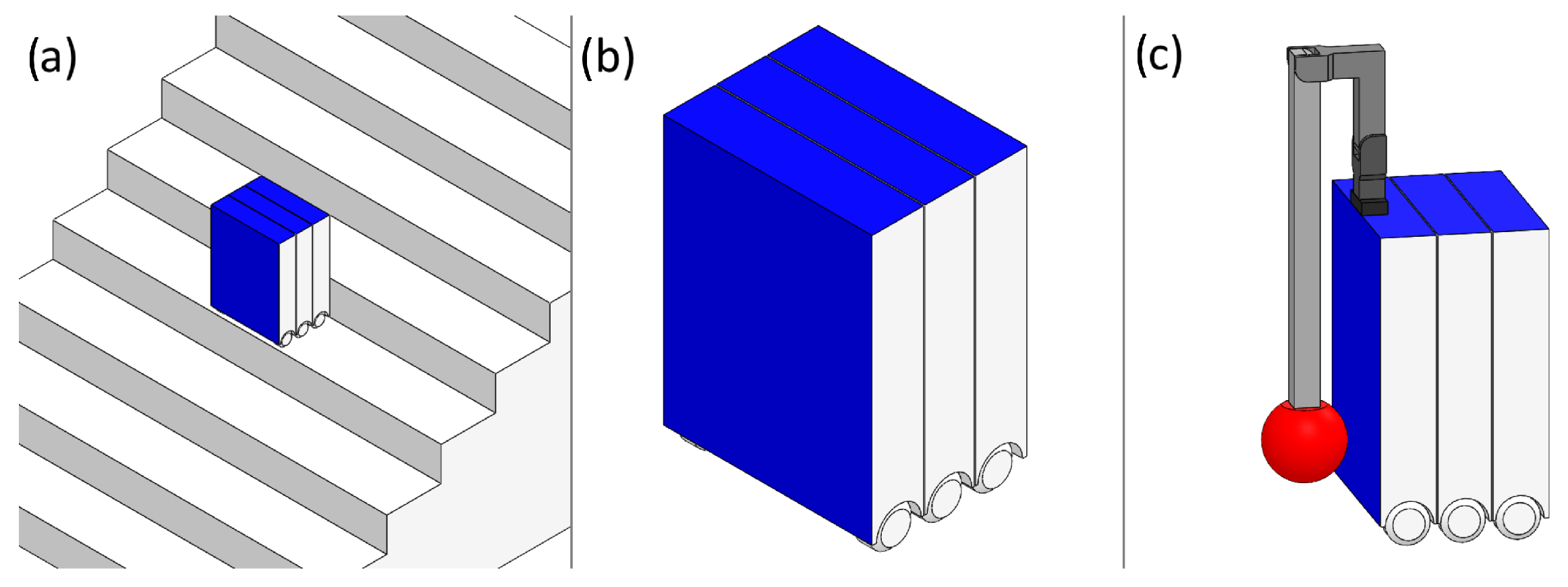
Figure 13.
(a) Model of proposed environment with service robot mockup. (b) Service robot close-up with available mounting area (c) Proposed fall damage mitigation system (3DoF arm).
Figure 13.
(a) Model of proposed environment with service robot mockup. (b) Service robot close-up with available mounting area (c) Proposed fall damage mitigation system (3DoF arm).
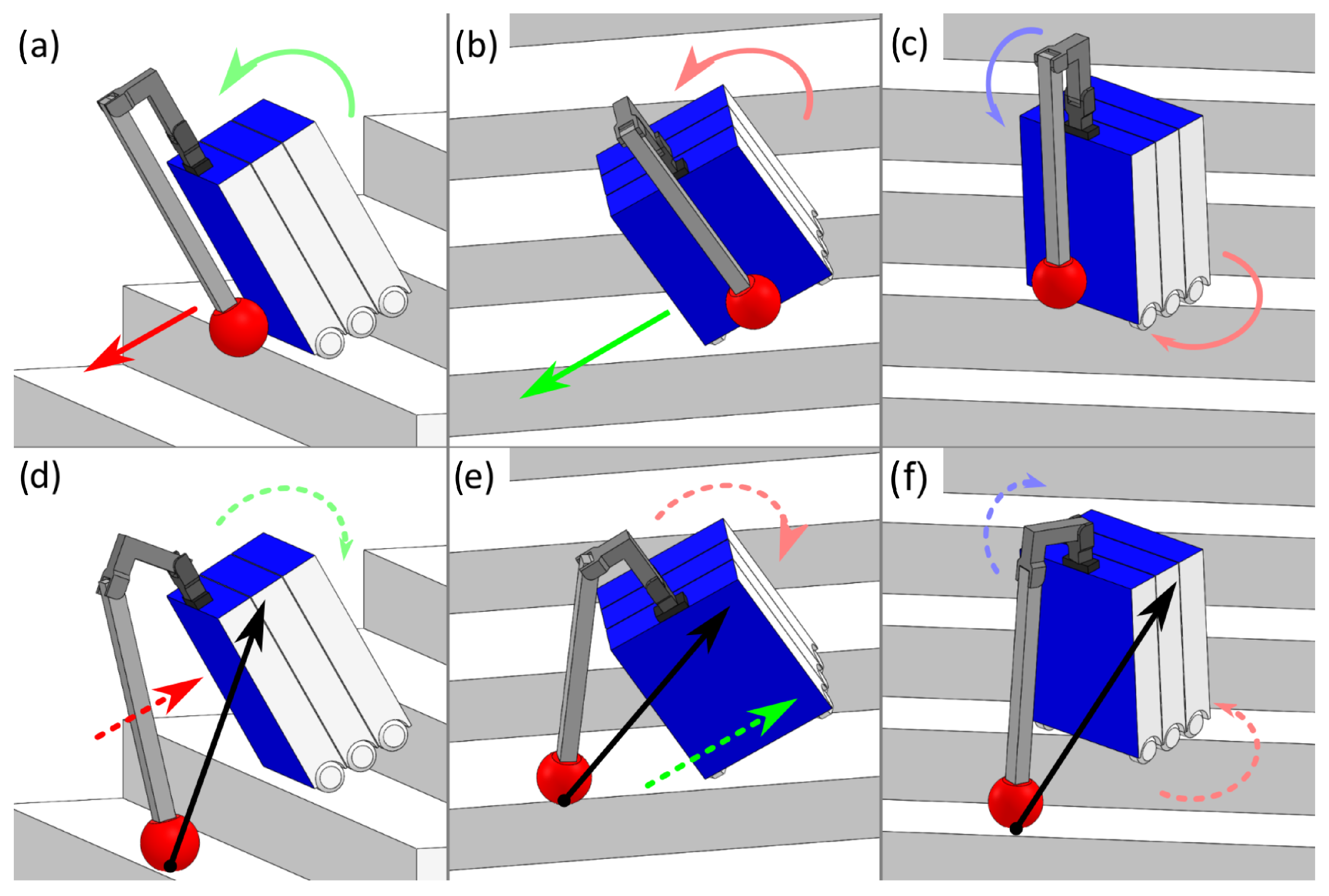
Figure 14.
Falls and the theoretical effects of the mitigation measures. With reference to the robot, linear movement along the x-axis are represented in red and rotational movement about the x-axis is represented in pink, linear movement along the y-axis are represented in green and rotational movement about the y-axis is represented in light green, and linear movement along the z-axis are represented in blue and rotational movement about the z-axis is represented in light blue. The black arrow illustrates the force acting on the robot as a result of the arm’s end effector making contact with the stairs. (a) Wrench for the BF fall scenario. (b) Wrench for the LF fall scenario. (c) Wrench for the CW fall scenario. (d) Arm movement and resulting wrench for the BF fall scenario. (e) Arm movement and resulting wrench for the LF fall scenario. (f) Arm movement and resulting wrench for the CW fall scenario.
Table 1.
Method of force application for each class of fall.
Table 1.
Method of force application for each class of fall.
| Class | Method |
|---|
| NF | Lightly shaking and pushing the physical prototype without it falling |
| LF | Pushing the prototype from the right to result in a fall |
| RF | Pushing the prototype from the left to result in a fall |
| CCW | Pulling the prototype from the top left edge backwards to result in a fall |
| CW | Pulling the prototype from the top right edge backwards to result in a fall |
| BF | Pulling the prototype from the top backwards to result in a fall |
Table 2.
Magnitude and position of the force applied on the virtual model for each class along the x-, y- and z-axes. The resulting force will be a force with randomized magnitude, angle, and position within a defined range on the surface of the model. The minimum magnitudes are determined by the least amount of force needed to cause a fall at the point of the least leverage, i.e., the lowest point where a force is applied, with the maximum being set as twice the minimum force. For forces that do not contribute to the fall of its class, a range of −3.0 N to 3.0 N is defined to provide some variance between the samples. The range of locations for force application is determined by places the robot is likely to get hit, namely the top half of its front and side faces.
| | Position [m] | Magnitude [N] |
|---|
| | x | y | z | x | y | z |
| BF | 0.14 | −0.10 to 0.10 | 0.15 to 0.25 | −42.0 to −21.0 | −3.0 to 3.0 | −3.0 to 3.0 |
| LF | −0.1 to 0.1 | −0.17 | 0.15 to 0.25 | −3.0 to 3.0 | 27.0 to 54.0 | −3.0 to 3.0 |
| RF | −0.1 to 0.1 | 0.17 | 0.15 to 0.25 | −3.0 to 3.0 | −54.0 to −27.0 | −3.0 to 3.0 |
| NF | 0.14 | −0.17 to 0.17 | −0.25 to 0.25 | −15 to 0 | −15 to 15 | −15 to 15 |
| CCW | 0.14 | −0.17 to −0.15 | 0.15 to 0.25 | −42.0 to −21.0 | 10.0 to 25.0 | −3.0 to 3.0 |
| CW | 0.14 | 0.15 to 0.17 | 0.15 to 0.25 | −42.0 to −21.0 | −25.0 to −10.0 | −3.0 to 3.0 |
Table 3.
Time taken from force application to fall, in seconds. The shortest time to fall (0.4 s for LF) is bolded.
Table 3.
Time taken from force application to fall, in seconds. The shortest time to fall (0.4 s for LF) is bolded.
| | #1 | #2 | #3 | #4 | #5 | #6 | #7 | #8 | #9 | #10 | #11 | #12 | #13 | #14 | #15 | #16 | #17 | #18 | #19 | #20 | Mean | Minimum |
|---|
| BF | 0.6 | 0.67 | 1.1 | 0.6 | 1.53 | 0.7 | 1.13 | 0.5 | 0.53 | 0.8 | 0.8 | 0.53 | 0.57 | 0.7 | 1.17 | 0.57 | 0.5 | 0.53 | 0.77 | 0.5 | 0.74 | 0.5 |
| LF | 0.87 | 0.43 | 0.97 | 0.53 | 0.53 | 0.47 | 0.4 | 0.73 | 0.97 | 0.5 | 0.47 | 0.9 | 0.6 | 0.63 | 0.97 | 0.53 | 0.5 | 0.63 | 0.63 | 0.47 | 0.6365 | 0.4 |
| RF | 0.6 | 0.57 | 0.73 | 0.77 | 0.87 | 0.73 | 0.67 | 0.83 | 0.77 | 0.87 | 0.63 | 0.7 | 0.53 | 0.53 | 0.57 | 0.7 | 0.73 | 0.9 | 0.5 | 0.5 | 0.685 | 0.5 |
| CCW | 0.67 | 0.57 | 0.6 | 0.5 | 0.57 | 0.6 | 0.7 | 0.6 | 0.53 | 0.53 | 0.57 | 0.53 | 1.87 | 0.67 | 0.67 | 0.63 | 0.67 | 0.57 | 0.57 | 0.83 | 0.6725 | 0.5 |
| CW | 0.6 | 1.03 | 0.6 | 0.57 | 0.93 | 0.6 | 0.63 | 0.63 | 0.67 | 0.6 | 0.67 | 0.9 | 0.7 | 0.6 | 0.63 | 0.6 | 0.57 | 0.73 | 0.73 | 0.67 | 0.683 | 0.57 |
Table 4.
Average accuracy for each hyperparameter value. The highest average accuracy for each hyperparameter is bolded and bracketed.
Table 4.
Average accuracy for each hyperparameter value. The highest average accuracy for each hyperparameter is bolded and bracketed.
| Frames | Features | Epochs | Cells |
|---|
| 6 | 9 | 12 | 10 | 15 | 20 | 60 | 80 | 100 | 100 | 150 | 200 |
| 85.614 | [88.085] | 85.899 | [87.234] | 86.640 | 85.724 | 86.523 | [86.546] | 86.529 | 86.513 | 86.512 | [86.573] |
Table 5.
The average accuracy of the LSTM models for each hyperparameter combination, with a color gradient applied to better visualize the results (green—high, red—low). The average accuracy of the chosen hyperparameter combination is bolded and bracketed. The highest average accuracy is underlined and italicized.
| EPOCH | 60 | 80 | 100 |
|---|
| CELL | 100 | 150 | 200 | 100 | 150 | 200 | 100 | 150 | 200 |
| 6 Frames | 10 Features | 86.227 | 86.139 | 86.489 | 85.963 | 86.139 | 86.665 | 85.964 | 86.541 | 86.400 |
| 15 Features | 85.700 | 85.611 | 85.788 | 85.875 | 85.699 | 85.961 | 85.174 | 85.874 | 85.876 |
| 20 Features | 84.385 | 84.999 | 85.000 | 84.560 | 85.000 | 84.737 | 84.911 | 85.086 | 84.824 |
| 9 Frames | 10 Features | 88.511 | 88.508 | 88.333 | 87.983 | 87.983 | [88.247] | 88.510 | 87.983 | 87.756 |
| 15 Features | 88.072 | 88.686 | 88.686 | 88.685 | 88.071 | 88.773 | 88.334 | 88.511 | 88.423 |
| 20 Features | 88.423 | 86.928 | 87.456 | 87.193 | 87.368 | 87.367 | 87.893 | 87.367 | 88.245 |
| 12 Frames | 10 Features | 86.928 | 87.455 | 87.016 | 87.456 | 86.928 | 87.631 | 87.104 | 87.368 | 87.104 |
| 15 Features | 85.875 | 85.876 | 85.347 | 86.313 | 85.614 | 85.788 | 85.525 | 85.699 | 85.439 |
| 20 Features | 84.912 | 84.824 | 83.948 | 84.735 | 84.911 | 85.087 | 84.648 | 84.649 | 85.088 |


