Correctness of Fuzzy Inference Systems Based on f-Inclusion

Abstract

Recent work has shown that the f-index of inclusion can serve as a foundation for modeling Generalized Modus Ponens. In this paper, we develop a novel fuzzy inference system based on this inference rule. To establish its soundness, we connect it to a Fuzzy Description Logic $\mathcal{LU}$ enriched with fuzzy modifiers (also known as fuzzy hedges). This logic background provides to the approach a strength absent in most fuzzy inference systems in the literature, which allows us to formally prove a series of results that culminate in a final correctness theorem for the proposed fuzzy inference system. This paper also presents a running example aimed at showing the potential applicability of the proposal.

1. Introduction

Fuzzy inference rules have long served as a cornerstone in fuzzy set theory, bridging theoretical concepts with practical applications. There are two main kinds of fuzzy inference systems (FISs) according to how the inference is performed. The first group is formed by the so-called relational fuzzy inference systems and includes the well-known compositional rule of inference, which performs an inference by means of a fuzzy relation and a couple of fuzzy operators, standardly, a fuzzy conjunction and a fuzzy implication. In this group, the most prominent approach is the one of Mamdani [1], but we can find in the literature more general approaches [2,3,4]. On the other hand, the second group of approaches is formed by those whose rules provide crisp values which are combined by means of aggregator operators in order to obtain a final inference. In this latter group, the most prominent approaches are those of Takagi–Sugeno [5] and Tsukamoto’s FIS [6], although some other recent FISs in this family can be found as well, such as those based on F-transforms [7], those considering probability distributions as consequents [8], or those considering nonlinear systems as consequents [9].

While their utility is undeniable (e.g., there are recent approaches dealing with Multicriteria Decision-Making [10,11] or medical diagnosis [12]), a critical flag remains from a theoretical point of view. Rigorously speaking, most of the FISs in the literature are not developed on the basis of a formal fuzzy logic system. In other words, although those FISs rely on fuzzy logic operators, they lack the formal syntax and semantics necessary for a rigorous definition of the notion of consequence. This absence impedes the ability to formally define syllogisms and to prove the correctness of those inference processes. As a result, the literature on FISs focuses mainly on appropriateness rather than on logical correctness. Here are some illustrative examples: in [8], the appropriateness of fuzzy-probabilistic inference systems is measured according to empirical experimentation with ad hoc data and real data; in [7], the appropriateness of dependency rules is rephrased in terms of results that prove the representation of functions via F-transforms; in [3], the appropriateness of relational fuzzy inference rules is reduced to the satisfiability of fuzzy relational equations; and in [9], the appropriateness of a switching Takagi–Sugeno FIS is identified with results on stability.

Most FISs are based on approximate reasoning and the so-called Generalized Modus Ponens (GMP). GMP is a conceptual inference that extends the Modus Ponens syllogism as follows: given $X\to Y$ and something similar to X (denoted by $X^{\prime }$), we can infer something similar to Y (denoted by $Y^{\prime }$). This inference rule is usually depicted as

$$\begin{array}{c}X\to Y\\ \frac{X^{\prime }}{\therefore Y^{\prime }}\end{array}$$

(1)

Taking this as the reference point, we present in this paper a novel FIS that makes use of a GMP recently defined by means of the f-inclusion [13] between fuzzy sets [14].

Remarkably, both components needed in the definition of the GMP can be modeled by f-inclusion. This is due to a dual interpretability of this operator. On the one hand, in [15], we proved that f-inclusion can be linked to an optimal choice of an implication operator in order to perform a Modus Ponens. Consequently, this operator can be interpreted as the truth degree of an If–Then rule. On the other hand, f-inclusion was originally designed to represent inclusion, but then, it was also appropriated to represent similarity between two fuzzy sets [16].

The proposed FIS is defined as a formal logic system by means of a syntactic construction of rules and a semantics, i.e., models. The semantics is based on Fuzzy Description Logic [17], a family of formal logics that represents knowledge and reasons with it by using as central element the notion of inclusion between fuzzy sets. This link with Fuzzy Description Logic allows us to prove that the GMP used in our FIS is a correct inference rule; in other words, our FIS performs correct inferences even if the input (a fuzzy set) does not coincide with the antecedents of rules.

It is worth mentioning here the two main differences of our approach with respect to the compositional rule of inference.

• The compositional rule of inference requires a fuzzy relation to link the universes of X and Y and to compute the output. In our approach, the connection between universes is left to interpretations and models. This simplifies the computation of the output in our FIS.
• The compositional rule of inference requires to fix a pair of operators in advance, in general, an implication operator and a conjunction operator. However, we do not need to fix operators in advance; the inference is performed directly by a mapping that represents the inclusion between fuzzy sets.

These two facts make our approach simpler and more interpretable than the traditional FISs.

It is also worth mentioning here two approaches that deal with providing a formal logical sustain to FIS. The first is [18], which shows that most of the deduction procedures appearing in FISs can be axiomatized in Rational Pavelka Predicate Logic. The other is [4], where the author presents an FIS based on a formal fuzzy logic system with its respective syntax and semantics. The main difference between those approaches and the FIS based on f-inclusions is that the logic theory supporting the latter is Description Logic, which is a much more application-oriented logic theory than Rational Pavelka Predicate Logic [19] (used in [18]) and the ${\mathrm{MTLF}}_{\Delta }$ [20] (used in [4]). This fact makes our approach more application-oriented than [4].

This paper is structured as follows: In Section 2, we present some preliminary notions that are used throughout the paper. Subsequently, in Section 3, we introduce the Description Logic ${\mathcal{LU}}_{FH}$, which allows us to consider intersection, union, and concept modifiers (or fuzzy hedges) in the syntax. The semantics provided for modifiers in our approach differs slightly from the one presented in [21], since here, we require them to be part of an adjoint pair. This modification allows us to define a correct GMP in ${\mathcal{LU}}_{FH}$ through the adjunction property. Section 4 contains the main content of the paper, the FIS based on the notion of f-inclusion. Such a section describes the syntax and semantics of knowledge databases, allowing us to formally define the concept of consequence. In this section, we also present a link between models of knowledge databases and those of the Description Logic ${\mathcal{LU}}_{FH}$, allowing us to use any inference of ${\mathcal{LU}}_{FH}$ on our knowledge databases. Throughout this section, we provide an illustrative example that shows the semantics and the performance of our FIS. Finally, in Section 6, we present some conclusions and future works.

2. Preliminaries

Let us begin by recalling the notion of fuzzy set.

Definition 1.

A fuzzy set is a pair $A=(\mathcal{U},{\mu }_A)$ where $\mathcal{U}$ is a non-empty set (called universe) and ${\mu }_A$ a mapping from $\mathcal{U}$ to $[0,1]$ (called membership function).

The set of fuzzy sets defined on the universe $\mathcal{U}$ is denoted by $\mathcal{F}\left(\mathcal{U}\right)$. Moreover, since the universe is in general pre-fixed by the context, for the sake of clarity, we refer to a fuzzy set $(\mathcal{U},{\mu }_A)$ directly by its membership function, i.e., $A\left(u\right)={\mu }_A\left(u\right)$.

Let us recall that a fuzzy partition of a universe $\mathcal{U}$ is a set $P=\{A_1,A_2,\dots ,A_n\}$ of fuzzy sets on $\mathcal{U}$ satisfying the covering property, i.e., for all $u\in \mathcal{U}$, there exists a fuzzy set $A_i\in P$ such that $A_i\left(u\right)>0$. In this paper, we also use the notions of the core and support of a fuzzy set.

Definition 2.

Given $A\in \mathcal{F}\left(\mathcal{U}\right)$, the support of A is defined as

$$supp\left(A\right)=\{u\in \mathcal{U}|{\mu }_A\left(u\right)>0\}$$

and the core of A is defined as

$$core\left(A\right)=\{u\in \mathcal{U}|{\mu }_A\left(u\right)=1\}.$$

Zadeh identified the ordering between fuzzy sets with the ordering of their membership functions, i.e., $A\le B$ if and only if ${\mu }_A\left(u\right)\le {\mu }_B\left(u\right)$ for all $u\in \mathcal{U}$. Because this relation is quite restrictive and rigid, many authors have focused on generalizing the ordering between fuzzy sets with a graduated structure. In this paper, we focus on the f-index of inclusion, which is a novel notion that identify the ordering between fuzzy sets via a mapping from $[0,1]$ to $[0,1]$. Not any mapping from $[0,1]$ to $[0,1]$ is appropriate to represent such an inclusion, so the first step is to fix the set of possible functions used as indexes.

Definition 3.

The set of indexes of inclusion, denoted by Ω, consists of all the deflationary and monotonically increasing mappings, that is, any mapping $f:[0,1]\to [0,1]$ such that

• $f\left(x\right)\le x$ for all $x\in [0,1]$;
• $x\le y$ implies $f\left(x\right)\le f\left(y\right)$ for all $x,y\in [0,1]$.

The indexes of inclusion are assigned by means of the notion of f-inclusion recalled below.

Definition 4.

Let A and B be two fuzzy sets and consider $f\in \Omega$. We say that A is f-included in B, denoted by $A{\subseteq }_{f}B$, if and only if the inequality $f\left(A\right(u\left)\right)\le B\left(u\right)$ holds for all $u\in \mathcal{U}$.

Here, it is convenient to note that each mapping $f\in \Omega$ determines a different restriction by means of f-inclusion; in other words, given a fuzzy set A, the greater $f\in \Omega$, the stronger the restriction imposed on the fuzzy set B by the f-inclusion. The reader is referred to [13,16] for more details about that assertion. Finally, the f-index of inclusion between two fuzzy sets is determined by choosing an index in $\Omega$ that represents the criterion given by the f-inclusion. Instead of presenting the original one [13], we consider here a recent generalization [22,23], which allows us to consider subsets of $\Omega$ to determine such a choice.

Definition 5.

Let A and B be two fuzzy sets and Θ be a join-subsemilattice of Ω, i.e., Θ is closed under arbitrary suprema and contains $\mathbf{0}$ and id. Then, the f-index of inclusion restricted to Θ, denoted by ${Inc}_{\Theta }(A,B)$, is defined as

$${Inc}_{\Theta }(A,B)=sup\{f\in \Theta \mid A{\subseteq }_{f}B\}.$$

If $\Theta =\Omega$, we write directly $Inc(A,B)$ to denote the f-index of inclusion. In [22], the properties of the f-index of inclusion were studied according to the axiomatic properties required by the standard approaches of inclusion between fuzzy sets [24,25]. We refer the reader to [16] for a detailed explanation on how to compute the f-index of inclusion.

Theorem 1.

Let $A,B$, and C be three fuzzy sets and let $\Theta \subseteq \Omega$ be a join-subsemilattice of Ω with $\mathbf{0},id\in \Theta$; then,

1. 

${Inc}_{\Theta }(A,B)\le Inc(A,B)$;

2. 

${Inc}_{\Theta }(A,B)=id$ if and only if $A\left(u\right)\le B\left(u\right)$ for all $u\in \mathcal{U}$;

3. 

${Inc}_{\Theta }(A,B)=\mathbf{0}$ if and only if, for each $f\in \Theta$ with $f\ne \mathbf{0}$, there exists an element $u\in \mathcal{U}$ such that $f\left(A\right(u\left)\right)>B\left(u\right)$;

4. 

$Inc(A,B)=\mathbf{0}$ if and only if there exists a set ${\left\{u_i\right\}}_{i\in \mathcal{I}}\subseteq \mathcal{U}$ such that $A\left(u_i\right)=1$ and ${inf}_{i\in \mathcal{I}}B\left(u_i\right)=0$;

5. 

If Θ is closed under composition (i.e., for all $f,g\in \Theta$, we have $f\circ g\in \Theta$), then $In{c}_{\Theta }(B,C)\circ In{c}_{\Theta }(A,B)\le In{c}_{\Theta }(A,C)$;

6. 

If $B\left(u\right)\le C\left(u\right)$ for every $u\in \mathcal{U}$, then $In{c}_{\Theta }(C,A)\le In{c}_{\Theta }(B,A)$;

7. 

If $B\left(u\right)\le C\left(u\right)$ for every $u\in \mathcal{U}$, then $In{c}_{\Theta }(A,B)\le In{c}_{\Theta }(A,C)$;

8. 

Let $T:\mathcal{U}\to \mathcal{U}$ be a bijective mapping on $\mathcal{U}$; then, $In{c}_{\Theta }(A,B)=In{c}_{\Theta }(T\left(A\right),T\left(B\right))$;

9. 

$In{c}_{\Theta }(A,B\cap C)\ge inf\{In{c}_{\Theta }(A,B),In{c}_{\Theta }(A,C)$};

10. 

$In{c}_{\Theta }(A\cup B,C)\ge inf\{In{c}_{\Theta }(A,C),In{c}_{\Theta }(B,C)$}.

Among all the join-semilattices of $\Omega$, the following one, denoted by $\mathcal{G}$, is remarkable, and it is used throughout the paper.

Definition 6.

The set $\mathcal{G}$ contains all the mappings in $f\in \Omega$ satisfying that there exists $g:[0,1]\to [0,1]$ such that $(f,g)$ is an adjoint pair.

Let us recall that an adjoint pair $(f,g)$ in $[0,1]$ is a pair of functions $f,g:[0,1]\to [0,1]$ such that

$$f\left(x\right)\le y\iff x\le g\left(y\right)$$

for all $x,y\in [0,1]$. This property (called adjointness) is used in this paper to define a Generalized Modus Ponens that is used as the inference engine of our fuzzy inference system. It is worth recalling here a well-known result about adjoint pairs [26]. With a fixed mapping $f:[0,1]\to [0,1]$, there exists a mapping $g:[0,1]\to [0,1]$ such that $(f,g)$ forms an adjoint pair if and only if f is left continuous. Moreover, in this case, the mapping g is unique and right continuous.

3. The Description Logic with Concept Modifiers ${\mathcal{LU}}_{\mathit{F}\mathit{H}}$

In this section, we provide the syntax and semantics of the Description Logic ${\mathcal{LU}}_{FH}$ that adds to the standard syntax of $\mathcal{LU}$ fuzzy modifiers (or fuzzy hedges). Thanks to these modifiers, which are interpreted as mappings in $\mathcal{G}$ (Definition 6), we can define a correct Generalized Modus Ponens (GMP) in ${\mathcal{LU}}_{FH}$. Later, in Section 4, we use this Description Logic as the reference to define our inference engine.

3.1. Syntax of ${\mathcal{LU}}_{FH}$

The formal language of ${\mathcal{LU}}_{FH}$ consists of a set of alphabets of symbols, for individuals, concepts, modifiers, and membership degrees.

• The set of individuals is represented by lowercase letters $a,b,c,\dots$. In general, they are denoted by $a_i$.
• The set of primitive concepts, identified by uppercase letters $A,B,\dots$ ($A_i$ in general), denote properties satisfied by individuals. Here, we also include two particular concepts, the top (⊤) and bottom (⊥) concepts.
• The set of truth-depressing modifiers is denoted by the symbol $m_i$.
• The set of membership degrees is represented through Greek letters $\alpha ,\beta ,\dots$ (in general, ${\alpha }_i$).

On the other hand, this syntax also includes the connectives ⊓, ⊔, ⊑, ∘, and −. Specifically, given a truth-depressing modifier m, we can construct a new modifier called truth-stressing modifier as follows:

$$\begin{array}{cc}\hfill \overline{m} \mid & (\mathrm{truth}\text{-}\mathrm{stressing}\mathrm{modifier})\hfill \end{array}$$

Note that by construction, the operator − cannot be applied twice to one modifier, since it is applied directly on truth-depressing modifiers, which are atomic elements in the alphabet. Moreover, given two (truth-stressing or truth-depressing) modifiers $m_1$ and $m_2$, the following expression is a modifier as well:

$$\begin{array}{cc}\hfill m_1\circ m_2 \mid & (\mathrm{composition}\mathrm{of}\mathrm{modifiers})\hfill \end{array}$$

Finally, given two concepts C and D and one modifier m, the following expressions are concepts as well:

$$\begin{array}{cc}\hfill C\sqcap D \mid & (\mathrm{concept}\mathrm{conjunction})\hfill \\ \hfill C\bigsqcup D \mid & (\mathrm{concept}\mathrm{disjunction})\hfill \\ \hfill {}^{m}C \mid & (\mathrm{modified}\mathrm{concept})\hfill \end{array}$$

The interpretation of the connectives ⊓, ⊔, ⊑, ∘, and − is left to the following section, which is devoted to the semantics of ${\mathcal{LU}}_{FH}$. Moreover, the auxiliary symbols ⟨ and ⟩ are also used in this syntax to define the following axioms.

Definition 7

([17]). Given a concept C and an individual a, an assertion is an expression of type $C\left(a\right)$, where a is called instance of C. A fuzzy assertion is a pair $⟨C\left(a\right),\alpha ⟩$, where $C\left(a\right)$ is an assertion and $\alpha \in [0,1]$.

A fuzzy assertion $⟨C\left(a\right),\alpha ⟩$ is an expression that can be translated as “the membership degree of a being an instance of C is at least $\alpha$”. A finite set of fuzzy assertions is called an A-Box, which is denoted by $\mathbf{A}$.

Definition 8

([17]). A concept specialization or terminological axiom is a relation between two concepts C and D denoted by $C⊑D$.

A concept specialization $C⊑D$ is interpreted as “C is more specific than D”. A finite set of terminological axioms, denoted by $\mathbf{T}$, is called a T-Box.

Definition 9.

A set of axioms is an ordered pair $⟨\mathbf{T},\mathbf{A}⟩$ consisting of a T-Box and a A-Box.

Below, we present an example showing a T-Box and an A-Box contextualized on cars.

Example 1.

Let us consider the following T-Box, denoted by $\mathbf{T}$, aimed at describing the notions of a sports car and a family car.

$$\begin{array}{c}\hfill {}^{High}HorsePower\left(x\right)\sqcap Fast\left(x\right)⊑SportsCar\left(x\right)\\ \hfill {}^{High}HorsePower\left(x\right)\sqcap Small\left(x\right)\sqcap Light\left(x\right)⊑{}^{very}Fast\left(x\right)\\ \hfill big\_Interior\left(x\right)\sqcap big\_Trunk(x)⊑FamilyCar\left(x\right)\end{array}$$

Let us consider also the following A-box, $\mathbf{A}$, with instances about one hypothetical car a

$$\begin{array}{c}\hfill ⟨HorsePower\left(a\right);0.9⟩\\ \hfill ⟨Small\left(a\right);0.9⟩\\ \hfill ⟨Light\left(a\right);0.7⟩\end{array}$$

In order to obtain the consequences from the T-Box and the assertions in the A-Box, we need to define the semantics in ${\mathcal{LU}}_{FH}$, which is carried out in next section.

Table 1 presents a summary of the main symbols employed in this syntax along with their respective interpretation.

Table 1. Summary of connectors and modifiers included in ${\mathcal{LU}}_{FH}$.

Symbol	Label
⊤	Top concept
⊥	Bottom concept
$C\sqcap D$	Concept conjunction
$C\bigsqcup D$	Concept disjunction
$⟨C\left(a\right),\alpha ⟩$	Fuzzy assertion
$C⊑D$	Concept specialization
m	Truth-depressing modifier
$\overline{m}$	Truth-stressing modifier

3.2. Semantics of ${\mathcal{LU}}_{FH}$

Definition 10

([17]). A fuzzy interpretation (or simply an interpretation) $\mathcal{I}$ is a pair $\mathcal{I}=({\Delta }^{\mathcal{I}},{·}^{\mathcal{I}})$ such that ${\Delta }^{\mathcal{I}}$ is a non-empty set called domain, and ${·}^{\mathcal{I}}$ is an interpretation function mapping:

• Different individuals into different elements of ${\Delta }^{\mathcal{I}}$;
• Primitive concepts into membership degree functions ${\Delta }^{\mathcal{I}}\to [0,1]$;
• Truth-depressing modifiers into mappings in $\mathcal{G}$ (see Definition 6).

For convention, given an individual a, a primitive concept C, and a modifier m, the mappings given by a fuzzy interpretation $\mathcal{I}$ are denoted by $a^{\mathcal{I}},C^{\mathcal{I}}$ and $m^{\mathcal{I}}$, respectively. Moreover, note that fuzzy interpretations can be extended to concepts constructed by means of connectives and other symbols as follows:

$$\begin{array}{cc}\hfill {\top }^{\mathcal{I}}\left(u\right)& =1\hfill \\ \hfill {\perp }^{\mathcal{I}}\left(u\right)& =0\hfill \\ \hfill {(C\sqcap D)}^{\mathcal{I}}\left(u\right)& =min\{C^{\mathcal{I}}\left(u\right),D^{\mathcal{I}}\left(u\right)\}\hfill \\ \hfill {(C\bigsqcup D)}^{\mathcal{I}}\left(u\right)& =max\{C^{\mathcal{I}}\left(u\right),D^{\mathcal{I}}\left(u\right)\}\hfill \\ \hfill {{(}^{m}C)}^{\mathcal{I}}\left(u\right)& =m^{\mathcal{I}}\left(C^{\mathcal{I}}\left(u\right)\right)\hfill \end{array}$$

for all $u\in {\Delta }^{\mathcal{I}}$, and to modifiers constructed by composition and − as follows:

$$\begin{array}{cc}\hfill {(m_1\circ m_2)}^{\mathcal{I}}& ={\left(m_1\right)}^{\mathcal{I}}\circ {\left(m_2\right)}^{\mathcal{I}}\hfill \\ \hfill {\left(\overline{m}\right)}^{\mathcal{I}}& =\mathrm{the}\mathrm{only}\mathrm{mapping}f\mathrm{such}\mathrm{that}(m^{\mathcal{I}},f)\mathrm{is}\mathrm{an}\mathrm{adjoint}\mathrm{pair}.\hfill \end{array}$$

Now that the notion of interpretation has been introduced, the reader is aware of the reasons why we have called the atomic modifiers truth-depressing and those constructed by −truth-stressing. In more detail, given an interpretation $\mathcal{I}$ and a truth-depressing modifier m, $m^{\mathcal{I}}$ is a mapping in $\Omega$, so $m^{\mathcal{I}}\left(\alpha \right)\le \alpha$ for all $\alpha \in [0,1]$. On the other hand, by construction, the modifier ${\overline{m}}^{\mathcal{I}}$ satisfies ${\overline{m}}^{\mathcal{I}}\left(\alpha \right)\ge \alpha$ for all $\alpha \in [0,1]$. The former kind of modifiers are called truth-depressors in the literature, whereas the latter, truth-stressors [27].

Table 2 shows some examples of truth-depressing modifiers that appear in the literature [28,29] along with their associated truth-stressing modifiers.

Table 2. Examples of truth-depressing modifiers and their associated truth-depressing modifiers.

Truth-Depressing Modifiers		Truth-Stressing Modifiers
Label	Analytical Expression	Label	Analytical Expression
True	$m\left(\alpha \right)=\alpha$	True	$\overline{m}\left(\alpha \right)=\alpha$
Very true	$m\left(\alpha \right)={\alpha }^2$	Fairly true	$\overline{m}\left(\alpha \right)=\sqrt{\alpha }$
Extremely true	$m\left(\alpha \right)={\alpha }^5$	Slightly true	$\overline{m}\left(\alpha \right)=\sqrt[5]{\alpha }$
At most n-true	$m\left(\alpha \right)=\left\{\begin{array}{cc}\alpha & \mathrm{if}\alpha \le n\\ n& \mathrm{if}\alpha >n\end{array}\right.$	At most n-certain	$\overline{m}\left(\alpha \right)=\left\{\begin{array}{cc}\alpha & \mathrm{if}\alpha <n\\ 1& \mathrm{if}\alpha \ge n\end{array}\right.$
n-strictly true	$m\left(\alpha \right)=\left\{\begin{array}{cc}0& \mathrm{if}\alpha \le n\\ n& \mathrm{if}\alpha >n\end{array}\right.$	n-uncertain	$\overline{m}\left(\alpha \right)=\left\{\begin{array}{cc}n& \mathrm{if}\alpha <n\\ 1& \mathrm{if}\alpha \ge n\end{array}\right.$
At least n-true	$m\left(\alpha \right)=\left\{\begin{array}{cc}0& \mathrm{if}\alpha \le n\\ \alpha & \mathrm{if}\alpha >n\end{array}\right.$	At least n-uncertain	$\overline{m}\left(\alpha \right)=\left\{\begin{array}{cc}n& \mathrm{if}\alpha <n\\ \alpha & \mathrm{if}\alpha \ge n\end{array}\right.$

Definition 11.

An interpretation $\mathcal{I}$ satisfies a fuzzy assertion $⟨C\left(a\right),\alpha ⟩$ if and only if $\alpha \le C^{\mathcal{I}}\left(a^{\mathcal{I}}\right)$. Moreover, $\mathcal{I}$ is said to satisfy a concept specialization $C⊑D$ if and only if $C^{\mathcal{I}}\left(u\right)\le D^{\mathcal{I}}\left(u\right)$ for all $u\in {\Delta }^{\mathcal{I}}$ (i.e., $C^{\mathcal{I}}$ is lesser than or equal to $D^{\mathcal{I}}$ in Zadeh’s sense).

Definition 12.

An interpretation $\mathcal{I}$ is called a model of a set of axioms $⟨\mathbf{T},\mathbf{A}⟩$ if and only if $\mathcal{I}$ satisfies each element of $⟨\mathbf{T},\mathbf{A}⟩$.

Definition 13.

A set of axioms $⟨\mathbf{T},\mathbf{A}⟩$ entails a fuzzy assertion $⟨C\left(a\right),\alpha ⟩$, written $⟨\mathbf{T},\mathbf{A}⟩\vDash ⟨C\left(a\right),\alpha ⟩$, if and only if every model of $⟨\mathbf{T},\mathbf{A}⟩$ also satisfies $⟨C\left(a\right),\alpha ⟩$. Similarly, we say that $⟨\mathbf{T},\mathbf{A}⟩$ entails a concept specialization $C⊑D$, written $⟨\mathbf{T},\mathbf{A}⟩\vDash C⊑D$, if and only if every model of $⟨\mathbf{T},\mathbf{A}⟩$ also satisfies $C⊑D$.

Example 2.

Let us reconsider the T-Box  T  and the A-Box  A described in Example 1. Let us consider a model $\mathcal{I}=({\Delta }^{\mathcal{I}},{·}^{\mathcal{I}})$ of $⟨\mathbf{T},\mathbf{A}⟩$. Then, $\mathcal{I}$ satisfies:

$$\begin{array}{cc}\hfill 0.9& \le {HorsePower}^{\mathcal{I}}\left(a^{\mathcal{I}}\right)\hfill \\ \hfill 0.9& \le {Small}^{\mathcal{I}}\left(a^{\mathcal{I}}\right)\hfill \\ \hfill 0.7& \le {Light}^{\mathcal{I}}\left(a^{\mathcal{I}}\right)\hfill \end{array}$$

Consider the truth-depressing modifier ^High. This modifier is interpreted by the model as follows:

$${High}^{\mathcal{I}}\left(\alpha \right)={\alpha }^2$$

for every $\alpha \in [0,1]$. Then, if we apply this modifier to the first assertion of the A-Box, we obtain the new assertion ${⟨}^{High}HorsePower\left(a\right);0.81⟩$. By Definition 11 it can be proven that the fuzzy assertions ${⟨}^{very}Fast\left(a\right);0.7⟩$ and $⟨SportsCar\left(a\right);0.7⟩$ are consequences of $⟨\mathbf{T},\mathbf{A}⟩$.

The literature on Description Logic contains plenty of algorithms to derive consequences and concept specializations from a set of axioms $⟨\mathbf{T},\mathbf{A}⟩$. However, that is out of the scope of this paper, and we refer the reader to [17,21] for more details.

3.3. Generalized Modus Ponens in ${\mathcal{LU}}_{FH}$

The inclusion of modifiers in the syntax of ${\mathcal{LU}}_{FH}$ enables the formulation of new inference rules that extend beyond the standard Description Logic $\mathcal{LU}$. The first result shows a couple of tautologies in ${\mathcal{LU}}_{FH}$ involving modifiers.

Proposition 1.

Given a concept specialization C and a truth-depressing modifier m, we have that

• $\vDash {}^{m}C⊑C$;
• $\vDash C⊑{}^{\overline{m}}C$.

Proof. 

To prove the first item, we have to show that any interpretation $\mathcal{I}=({\Delta }^{\mathcal{I}},{·}^{\mathcal{I}})$ is a model of ${}^{m}C⊑C$. By definition of an interpretation, $m^I\in \mathcal{G}$, so $m^{\mathcal{I}}\left(\alpha \right)\le \alpha$ for all $\alpha \in [0,1]$. As a result, $m^{\mathcal{I}}\left(C\left(u\right)\right)\le C\left(u\right)$ for all $u\in {\Delta }^{\mathcal{I}}$.

To prove the second item, let us consider an interpretation $\mathcal{I}=({\Delta }^{\mathcal{I}},{·}^{\mathcal{I}})$; we see that $\mathcal{I}$ is a model of $C⊑{}^{\overline{m}}C$. By definition of an interpretation, ${\overline{m}}^{\mathcal{I}}$ is the right part of an adjoint pair $(m^{\mathcal{I}},{\overline{m}}^{\mathcal{I}})$ with $m^{\mathcal{I}}\in \mathcal{G}$. Since $m^{\mathcal{I}}\left(\alpha \right)\le \alpha$ for all $\alpha \in [0,1]$, we have by the adjoint property that $\alpha \le {\overline{m}}^{\mathcal{I}}\left(\alpha \right)$ for all $\alpha \in [0,1]$. As a result, $C\left(u\right)\le {\overline{m}}^{\mathcal{I}}\left(u\right)$ for all $u\in {\Delta }^{\mathcal{I}}$. □

The second result shows that the modifier connective − can be used in inferences of concept specializations.

Proposition 2.

Given two concept specialization C and D and a truth-depressing modifier m, we have that

• ${}^{m}C⊑D\vDash C⊑{}^{\overline{m}}D$.
• $C⊑{}^{\overline{m}}D\vDash {}^{m}C⊑D$.

Proof. 

Let us prove the first item. Let $\mathcal{I}=({\Delta }^{\mathcal{I}},{·}^{\mathcal{I}})$ be a model of ${}^{m}C⊑D$. Then, for all $u\in {\Delta }^{\mathcal{I}}$, we have that

$$m^{\mathcal{I}}\left(C^{\mathcal{I}}\left(u\right)\right)\le D^{\mathcal{I}}\left(u\right)$$

Since $m^{\mathcal{I}}\in \mathcal{G}$, then $(m^{\mathcal{I}},{\overline{m}}^{\mathcal{I}})$ forms an adjoint pair, which implies that

$$C^{\mathcal{I}}\left(u\right)\le {\overline{m}}^{\mathcal{I}}\left(D^{\mathcal{I}}\left(u\right)\right)$$

for all $u\in {\Delta }^{\mathcal{I}}$, and then $\mathcal{I}$ satisfies $C⊑{}^{\overline{m}}D$. The other item is proved similarly. □

The following results present various versions of Generalized Modus Ponens (GMP) within the ${\mathcal{LU}}_{FH}$ language. In this framework, the syllogism of GMP is comprised of a concept specialization, which serves the role of implication, and the instance of the antecedent is incorporated in the form of an assertion.

Theorem 2.

Let $⟨\mathbf{T},\mathbf{A}⟩$ be a set of axioms composed of $\mathbf{T}=⟨C⊑D⟩$ and $\mathbf{A}={⟨}^{m}C\left(a\right),\alpha ⟩$. Then, $⟨\mathbf{T},\mathbf{A}⟩\vDash {⟨}^{m}D\left(a\right),\alpha ⟩$.

Proof. 

Consider a model $\mathcal{I}$ of $⟨\mathbf{T},\mathbf{A}⟩$. By definition, $\mathcal{I}$ satisfies

• $\alpha \le m^{\mathcal{I}}\left(C^{\mathcal{I}}\left(a^{\mathcal{I}}\right)\right)$, where $m^{\mathcal{I}}\in \mathcal{G}$;
• $C^{\mathcal{I}}\left(u\right)\le D^{\mathcal{I}}\left(u\right)$ for all $u\in {\Delta }^{\mathcal{I}}$.

Specifically, $C^{\mathcal{I}}\left(a^{\mathcal{I}}\right)\le D^{\mathcal{I}}\left(a^{\mathcal{I}}\right)$. Since $m^{\mathcal{I}}\in \mathcal{G}$ is a monotonic mapping, from the previous inequality, we can obtain $\alpha \le m^{\mathcal{I}}\left(C^{\mathcal{I}}\left(a^{\mathcal{I}}\right)\right)\le m^{\mathcal{I}}\left(D^{\mathcal{I}}\left(a^{\mathcal{I}}\right)\right)$. In other words, $\mathcal{I}$ satisfies the assertion ${⟨}^{m}D\left(a\right),\alpha ⟩$. In conclusion, $⟨\mathbf{T},\mathbf{A}⟩\vDash {⟨}^{m}D\left(a\right),\alpha ⟩$. □

The second GMP considers a modifier in a concept specialization and an assertion free of modifier.

Theorem 3.

Let $⟨\mathbf{T},\mathbf{A}⟩$ be a set of axioms composed of $\mathbf{T}={⟨}^{m}C⊑D⟩$ and $\mathbf{A}=⟨C\left(a\right),\alpha ⟩$. Then, $⟨\mathbf{T},\mathbf{A}⟩\vDash {⟨}^{\overline{m}}D\left(a\right),\alpha ⟩$.

Proof. 

Consider a model $\mathcal{I}$ of $⟨\mathbf{T},\mathbf{A}⟩$. By Proposition 2, every model of ${⟨}^{m}C⊑D⟩$ equally satisfies $⟨C⊑{}^{\overline{m}}D⟩$. Therefore, we have

• $\alpha \le C^{\mathcal{I}}\left(a^{\mathcal{I}}\right)$;
• $C^{\mathcal{I}}\left(u\right)\le {\overline{m}}^{\mathcal{I}}\left(D^{\mathcal{I}}\left(u\right)\right)$ for all $u\in {\Delta }^{\mathcal{I}}$.

Specifically, the following chain of inequalities holds:

$$\alpha \le C^{\mathcal{I}}\left(a^{\mathcal{I}}\right)\le {\overline{m}}^{\mathcal{I}}\left(D^{\mathcal{I}}\left(a^{\mathcal{I}}\right)\right).$$

Namely, $\mathcal{I}$ satisfies the assertion ${⟨}^{\overline{m}}D\left(a\right),\alpha ⟩$. In conclusion, $⟨\mathbf{T},\mathbf{A}⟩\vDash {⟨}^{\overline{m}}D\left(a\right),\alpha ⟩$. □

The third GMP considers two concept modifiers: one of them appears in the antecedent of the concept specialization, and the other one is included in the instance of the antecedent.

Theorem 4.

Let $⟨\mathbf{T},\mathbf{A}⟩$ be a set of axioms composed of $\mathbf{T}={⟨}^{m_1}C⊑D⟩$ and $\mathbf{A}={⟨}^{m_2}C\left(a\right),\alpha ⟩$. Then, $⟨\mathbf{T},\mathbf{A}⟩\vDash {⟨}^{m_2\circ \overline{m_1}}D\left(a\right),\alpha ⟩$.

Proof. 

Let $\mathcal{I}$ be a model of $⟨\mathbf{T},\mathbf{A}⟩$. Then,

• $C^{\mathcal{I}}\left(a^{\mathcal{I}}\right)\le {\overline{m_1}}^{\mathcal{I}}\left(D^{\mathcal{I}}\left(a^{\mathcal{I}}\right)\right)$ for all $a^{\mathcal{I}}\in {\Delta }^{\mathcal{I}}$;
• $\alpha \le {m_2}^{\mathcal{I}}\left(C^{\mathcal{I}}\left(a^{\mathcal{I}}\right)\right)$.

Therefore, by using the monotonicity of ${m_2}^{\mathcal{I}}$, we have

$$\alpha \le {m_2}^{\mathcal{I}}\left(C^{\mathcal{I}}\left(a^{\mathcal{I}}\right)\right)\le {m_2}^{\mathcal{I}}\left({\overline{m_1}}^{\mathcal{I}}\left(D^{\mathcal{I}}\left(a^{\mathcal{I}}\right)\right)\right)=({m_2}^{\mathcal{I}}\circ {\overline{m_1}}^{\mathcal{I}})\left(D^{\mathcal{I}}\left(a^{\mathcal{I}}\right)\right),$$

in other words, $\mathcal{I}$ satisfies the assertion ${⟨}^{m_2\circ \overline{m_1}}D\left(a\right),\alpha ⟩$, so $⟨\mathbf{T},\mathbf{A}⟩\vDash {⟨}^{m_2\circ \overline{m_1}}D\left(a\right),\alpha ⟩$. □

In the following section, the latter rule is used to derive conclusions from an inference system by applying it as the core of an inference engine.

4. A Fuzzy Inference System Based on the $\mathit{f}$-Index of Inclusion

Although in the literature, we can find different versions of fuzzy inference systems, all of them can be divided, in general, in four steps: fuzzification, knowledge database, inference engine and defuzzification. The first step is the fuzzification process, where crisp data are transformed into fuzzy information. Usually, this step is performed by means of a fuzzy partition. The knowledge database comprises some knowledge by rules of the type If–Then. The inference engine is the central stage, where the fuzzy inference system takes the fuzzified input and returns an output by combining the input with the rules in the knowledge database. Finally, the defuzzification process takes the output of the inference engine (usually a fuzzy set) and returns a crisp output according to the applied context of the FIS. Next, we specify how these four phases are formalized in our inference system based on the f-index of inclusion. We start with the knowledge database, to show how the information is comprised in If–Then-type rules. Then, under the semantics of the rules in the knowledge database, the inference engine is introduced using the Description Logic ${\mathcal{LU}}_{FH}$ as support. Finally, the fuzzification and defuziffication are analyzed according to the previous consideration.

4.1. The Knowledge Database

Definition 14.

A frame is a tuple $(X,Y,{\mathcal{A}}_X,{\mathcal{B}}_Y)$ where X and Y are sets and ${\mathcal{A}}_X$ and ${\mathcal{B}}_Y$ are two fuzzy partitions over the universes X and Y, where ${\mathcal{A}}_X={\left\{A_i\right\}}_{i\in I}$ and ${\mathcal{B}}_Y={\left\{B_j\right\}}_{j\in J}$.

Definition 15.

A knowledge database ($KB$) on the frame $(X,Y,{\mathcal{A}}_X,{\mathcal{B}}_Y)$ is a set of rules of the form

$$⟨A_i\to B_j;f_{ij}⟩$$

where $A_i\in {\mathcal{A}}_X$, $B_j\in {\mathcal{B}}_Y$ and $f_{ij}\in \mathcal{G}$.

To provide an interpretation to the connection between the implication rule $A_i\to B_j$ and its associated function $f_{ij}$, we use the f-inclusion relation between fuzzy sets, as presented in the following definition.

Definition 16.

Let Γ be a $KB$ on the frame $(X,Y,{\mathcal{A}}_X,{\mathcal{B}}_Y)$. A subset of pairs $M\subseteq X\times Y$ is a model of Γ, if, for every rule $⟨A_i\to B_j;f_{ij}⟩\in \Gamma$, we have that $f_{ij}\left(A_i\left(x\right)\right)\le B_j\left(y\right)$ for all $(x,y)\in M$. The set of all models of Γ is denoted by ${\mathbb{M}}_{\Gamma }$.

The use of the f-inclusion to model implication rules in our frame $(X,Y,{\mathcal{A}}_X,{\mathcal{B}}_Y)$ is justified by the ability of this operator to serve as fuzzy implication, as explained in [15].

Note that a model of a $KB$ is a crisp set, i.e., a subset of $X\times Y$ is either a model or not. Consequently, with a fixed $KB$ $\Gamma$, we can consider in the set of models of $\Gamma$, ${\mathbb{M}}_{\Gamma }$, the standard order between sets and then analyze the structure of $({\mathbb{M}}_{\Gamma },\subseteq )$. The next result shows that $({\mathbb{M}}_{\Gamma },\subseteq )$ is a complete lattice:

Theorem 5.

Let Γ be a $KB$ on a frame $(X,Y,{\mathcal{A}}_X,{\mathcal{B}}_Y)$, and let ${\mathbb{M}}_{\Gamma }$ be the set of models of Γ. Then, ${\mathbb{M}}_{\Gamma }$ has a complete lattice structure with the standard order between sets.

Proof. 

Let us prove that both intersection and union of an arbitrary number of models are also models. Let ${\left\{M_i\right\}}_{i\in I}\subseteq {\mathbb{M}}_{\Gamma }$ be a subset of models of $\Gamma$ and let us begin by showing that

$${\mathbf{M}}_{\cup }=\bigcup _{i\in I}{M}_i$$

is a model. Let $(x,y)\in {\mathbf{M}}_{\cup }$, then, necessarily, there exists a model $\overline{M}\in {\left\{M_i\right\}}_{i\in I}$ such that $(x,y)\in \overline{M}$. As a result, for any rule $⟨A_i\to B_j;f_{ij}⟩$ in $\Gamma$, we have $f_{ij}\left(A_i\left(x\right)\right)\le B_j\left(y\right)$. In other words, ${\mathbf{M}}_{\cup }$ is a model.

The proof that shows that

$${\mathbf{M}}_{\cap }=\bigcap _{i\in I}{M}_i$$

is a model of $\Gamma$ is similar. □

Corollary 1.

Let Γ be a $KB$ on a frame $(X,Y,{\mathcal{A}}_X,{\mathcal{B}}_Y)$, and let ${\mathbb{M}}_{\Gamma }$ be the set of models of Γ. Then, the greatest element of $({\mathbb{M}}_{\Gamma },\subseteq )$, denoted by ${\mathbf{M}}_{\Gamma }$, is the join of every model of Γ, and the least model of $({\mathbb{M}}_{\Gamma },\subseteq )$ is the empty set.

The previous result highlights a substantial difference with respect to Description Logic and logic programming. In the aforementioned formal theories, the emphasis is placed on minimal models (the least model in logic programming or canonical models in DL). In our work, we focus on the maximal model, as it determines the possible pairs of points in $X\times Y$ that are consistent with its associated $KB$. Later, in Section 4.2, it is shown that we can reduce our analysis to the greatest model of $\Gamma$ to check correct inferences.

Below, we provide an illustrative example describing a knowledge database where the step-by-step construction of its greatest model is described. For the sake of showing the potential application of this inference system, it has been contextualized in pediatrics despite the synthetic nature of the example.

Example 3.

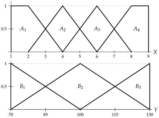
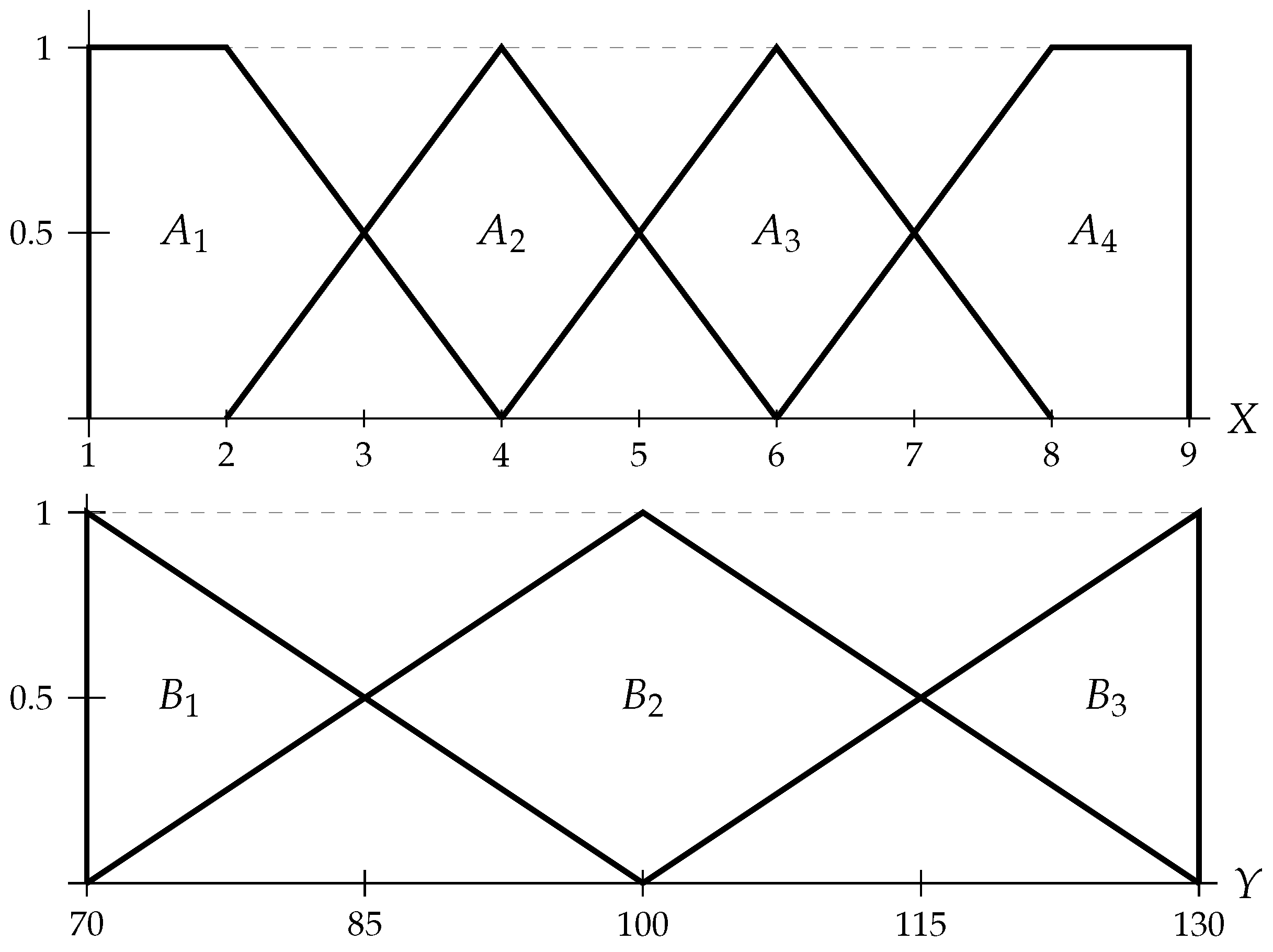
Let us assume that we have conducted a study on heart rate in infants and children between the ages of one and nine. In order to establish a relation between these two properties, we consider the frame $(X,Y,{\mathcal{A}}_X,{\mathcal{B}}_Y)$ consisting of

• The interval $X=[1,9]$ to represent the ages between 1 and 9, e.g., the age of an infant who is 18 months old would be $1.5$;
• The interval $Y=[70,130]$ to cover a wide range of heart rates (in bpm).

• The fuzzy partition ${\mathcal{A}}_X=\{A_1,A_2,A_3,A_4\}$ consists of four fuzzy sets $A_i\in \mathcal{F}\left(X\right)$ which distinguish four fuzzy age ranges. The membership functions corresponding to each element of ${\mathcal{A}}_X$ are

  $$A_1\left(x\right)=\left\{\begin{array}{cc}1& \mathit{if}x\in [1,2]\hfill \\ 2-0.5x& \mathit{if}x\in (2,4]\hfill \\ 0& \mathit{if}x\in (4,9],\hfill \end{array}\right.$$
  $$A_2\left(x\right)=\left\{\begin{array}{cc}0& \mathit{if}x\in [1,2]\hfill \\ 0.5x-1& \mathit{if}x\in (2,4]\hfill \\ 3-0.5x& \mathit{if}x\in (4,6]\hfill \\ 0& \mathit{if}x\in (6,9],\hfill \end{array}\right.$$
  $$A_3\left(x\right)=\left\{\begin{array}{cc}0& \mathit{if}x\in [1,4]\hfill \\ 0.5x-2& \mathit{if}x\in (4,6]\hfill \\ 4-0.5x& \mathit{if}x\in (6,8]\hfill \\ 0& \mathit{if}x\in (8,9],\hfill \end{array}\right.$$
  $$A_4\left(x\right)=\left\{\begin{array}{cc}0& \mathit{if}x\in [1,6]\hfill \\ 0.5x-3& \mathit{if}x\in (6,8]\hfill \\ 1& \mathit{if}x\in (8,9].\hfill \end{array}\right.$$
• The fuzzy partition ${\mathcal{B}}_Y=\{B_1,B_2,B_3\}$ only consists of three elements, which can be classified into $B_1$ = “low heart rate”, $B_2$ = “standard heart rate”, and $B_3$ = “high heart rate”, respectively. These fuzzy sets have the following respective associated membership functions:
  $$B_1\left(y\right)=\left\{\begin{array}{cc}{\displaystyle \frac{100-y}{30}}& \mathit{if}y\in [70,100]\hfill \\ 0& \mathit{if}y\in (100,130],\hfill \end{array}\right.$$
  $$B_2\left(y\right)=\left\{\begin{array}{cc}{\displaystyle \frac{y-70}{30}}& \mathit{if}y\in [70,100]\hfill \\ {\displaystyle \frac{130-y}{30}}& \mathit{if}y\in (100,130],\hfill \end{array}\right.$$
  $$B_3\left(y\right)=\left\{\begin{array}{cc}0& \mathit{if}y\in [70,100]\hfill \\ {\displaystyle \frac{y-100}{30}}& \mathit{if}y\in (100,130].\hfill \end{array}\right.$$

Both of these fuzzy partitions are represented in Figure 1.

Figure 1. Membership functions of every fuzzy set in ${\mathcal{A}}_X$ and ${\mathcal{B}}_Y$ in Example 3.

Once the frame $(X,Y,{\mathcal{A}}_X,{\mathcal{B}}_Y)$ has been defined, it is time to set the rules $⟨A_i\to B_j;f_{ij}⟩$ that constitute the knowledge base Γ. This $KB$ contains $4·3=12$ different rules, each one corresponding to a different combination of elements $A_i\in {\mathcal{A}}_X$ and $B_j\in {\mathcal{B}}_Y$. As explained before, the mapping $f_{ij}\in \mathcal{G}$ associated with each rule determines a relation of f-inclusion $A_i\to B_j$. In other words, when the relationship between $A_i$ and $B_j$ is stronger (i.e., patients with ages corresponding to $A_i$ tend to have a heart rate within $B_j$), the mapping $f_{ij}\in \mathcal{G}$ is closer to the identity (i.e., the f-inclusion relation is more restrictive). Conversely, when the elements $A_i$ and $B_j$ are not related at all, the inclusion function is null, i.e., $f_{ij}\left(\alpha \right)=\mathbf{0}\left(\alpha \right)=0$ for all $\alpha \in [0,1]$.

Since, in general, the average heart rate of infants and children decreases with age, the knowledge base associated with this frame is represented as in Table 3.

Table 3. $KB$ $\Gamma$ associated with $(X,Y,{\mathcal{A}}_X,{\mathcal{B}}_Y)$ in Example 3.

	$B_1$	$B_2$	$B_3$
$A_1$	$\mathbf{0}$	$\mathbf{0}$	$f_{0.5}$
$A_2$	$\mathbf{0}$	$f_{0.5}$	$g_{0.25}$
$A_3$	$\mathbf{0}$	$f_{0.75}$	$\mathbf{0}$
$A_4$	$f_{0.5}$	$\mathbf{0}$	$\mathbf{0}$

Where

$$g_n\left(\alpha \right)=\left\{\begin{array}{cc}0& if\alpha \le n\\ n& if\alpha >n,\end{array}\right.$$

$$f_n\left(\alpha \right)=\left\{\begin{array}{cc}\alpha & if\alpha \le n\\ n& if\alpha >n,\end{array}\right.$$

and $\mathbf{0}\left(\alpha \right)=0$ for all $\alpha \in [0,1]$.

Now that the $KB$ has been defined (denoted by Γ), it is time to compute its greatest model ${\mathbf{M}}_{\Gamma }$. Let us recall from Definition 16 that a model M of Γ is a set of pairs in $X\times Y$ which satisfy all the following f-inclusion relations:

$$f_{ij}\left(A_i\left(x\right)\right)\le B_j\left(y\right)$$

for every rule $⟨A_i\to B_j;f_{ij}⟩\in \Gamma$. Thus, in order to obtain the greatest model, we have to compute which pairs $(x,y)\in X\times Y$ satisfy each of these f-inclusions. This calculation can be performed graphically in the $X\times Y$ plane through the representation of all the restrictions imposed by each f-inclusion associated with each rule $⟨A_i\to B_j;f_{ij}⟩\in \Gamma$. This plotting process is performed step by step in order to facilitate its understanding.

Let us start by focusing on the second element of ${\mathcal{A}}_X$, $A_2$, which covers the fuzzy age range from 2 to 6 years. According to Table 3, the three rules associated with this fuzzy set are

$$⟨A_2\to B_1;\mathbf{0}⟩,\hspace{1em}\hspace{1em}⟨A_2\to B_2;f_{0.5}⟩,\hspace{1em}\hspace{1em}⟨A_2\to B_3;g_{0.25}⟩.$$

First of all, note that the former rule, $⟨A_2\to B_1;\mathbf{0}⟩$, does not impose any restriction on the set of models, since all pairs $(x,y)\in X\times Y$ satisfy null f-inclusions, i.e., $0=\mathbf{0}\left(A_2\left(x\right)\right)\le B_1\left(y\right)$. Therefore, the step-by-step graphical representation is only performed for the next two rules (since the graph associated to the first rule does not impose any constraint on the maximal model).

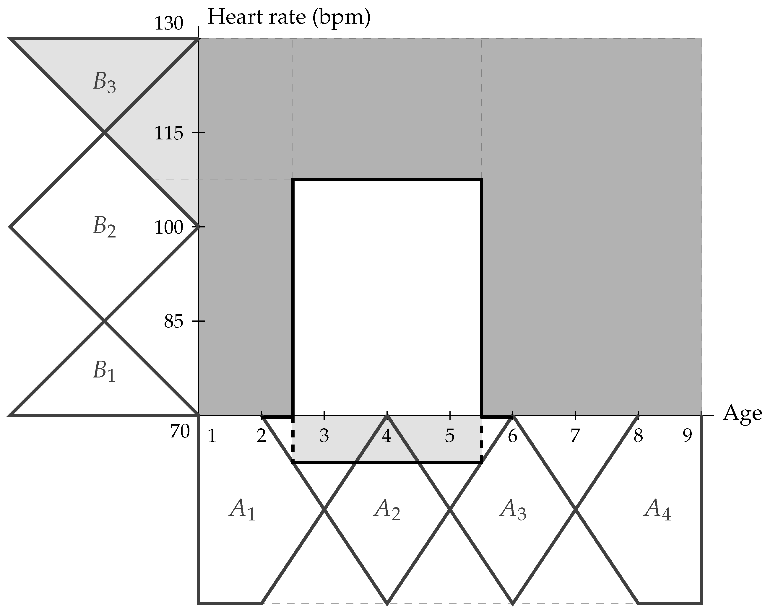
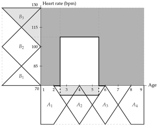
The graph in Figure 2 illustrates the pairs in $X\times Y$ that satisfy the condition imposed by the rule $⟨A_2\to B_2;f_{0.5}⟩$. This is carried out in two simple steps:

Figure 2. Graphical representation of rule $⟨A_2\to B_2;f_{0.5}⟩$ (bold line) in Example 3. Dashed lines are auxiliar lines and grey lines represent the partitions ${\mathcal{A}}_X$ and ${\mathcal{B}}_Y$. The shaded region represents the points which satisfy the rule.

• First, the fuzzy set $f_{0.5}\left(A_2\right)$ is computed, and its graph is represented over $A_2$ in the partition ${\mathcal{A}}_X$.
• Then, the pairs with positive membership degree in $A_2$ are selected. Among these, the pairs $(x,y)\in X\times Y$ whose y-coordinate has a membership degree in $B_2$ lower than $f_{0.5}\left(A_2\left(x\right)\right)$ are discarded from ${\mathbf{M}}_{\Gamma }$.

Note that the mapping $f_{0.5}$ associated with the rule $⟨A_2\to B_2;f_{0.5}⟩$ implies the existence of a patient whose age belongs to $A_2$ with the highest possible membership degree, that is, 4 years old, and with a heart rate with a membership degree in $B_2$ equal to $0.5$, e.g., 85 or 115 beats per minute.

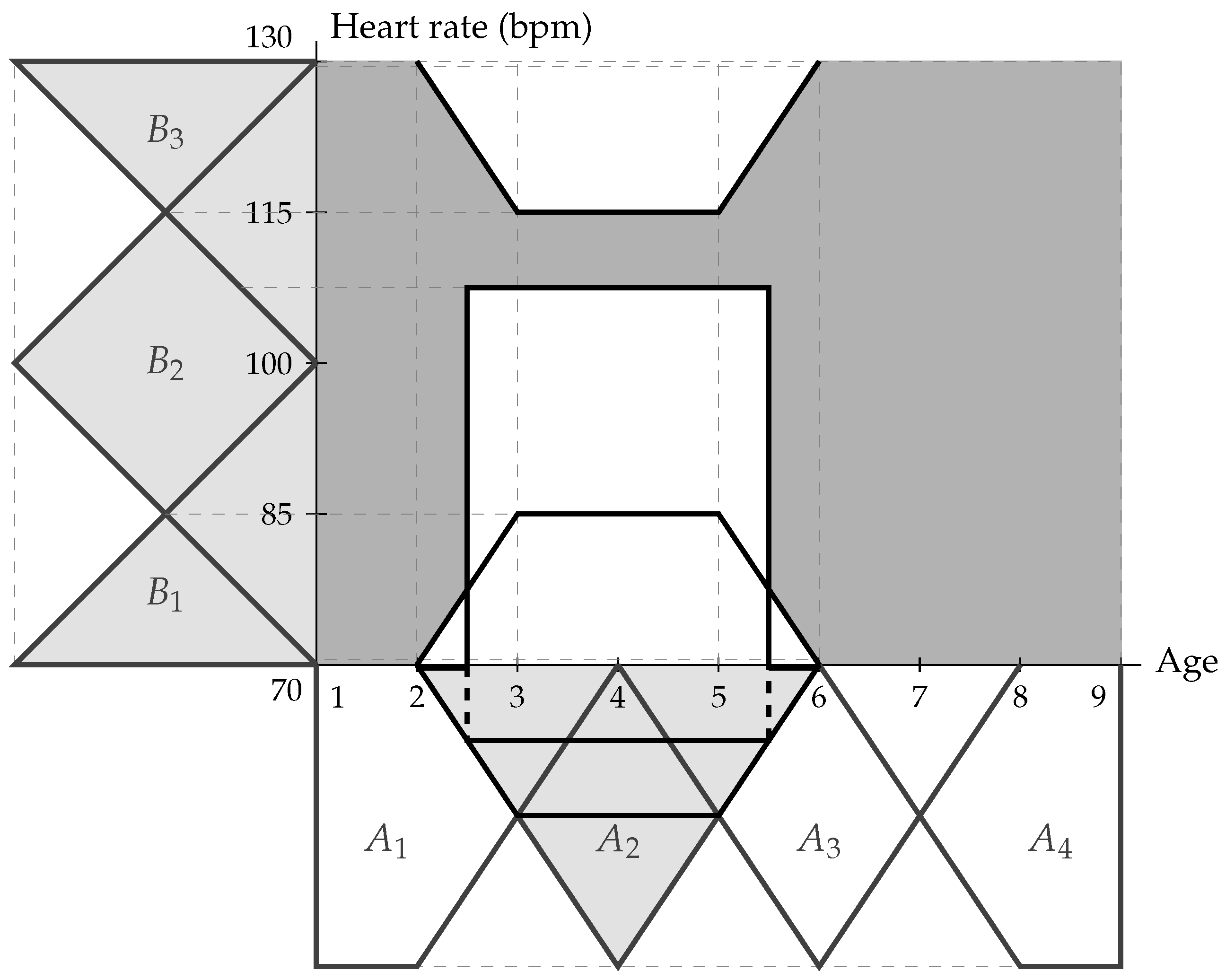
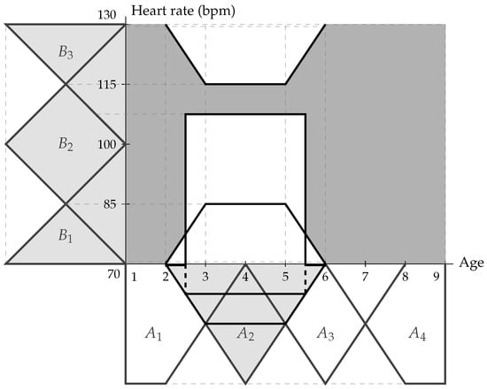
A similar process is followed to plot in Figure 3 the set of pairs $(x,y)\in X\times Y$ that satisfy the rule $⟨A_2\to B_3;g_{0.25}⟩$. The apparition of this mapping implies the existence of two different patients: one of them who is 4 years old and whose heart rate is approximately 110 and another one whose age has a membership degree in $A_2$ higher than $0.25$ (i.e., their age is between 30 and 66 months old) and whose heart rage is lesser or equal than 100 bpm, so it does not belong to partition $B_3$.

Figure 3. Graphical representation of rule $⟨A_2\to B_3;g_{0.25}⟩$ (bold line) in Example 3. Dashed lines are auxiliar lines and grey lines represent the partitions ${\mathcal{A}}_X$ and ${\mathcal{B}}_Y$. The shaded region represents the points which satisfy the rule.

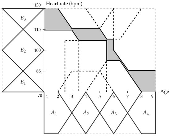
The final step consists in computing the intersection of the shaded regions obtained in Figure 2 and Figure 3, as the resulting region contains the set of pairs $(x,y)\in X\times Y$ that satisfy all the rules associated with the fuzzy set $A_2$. Figure 4 shows the result of this computation.

Figure 4. Graphical representation of rules $⟨A_2\to B_j;f_{2j}⟩$ for $j\in \{1,2,3\}$ (bold line) in Example 3. Dashed lines are auxiliar lines and grey lines represent the partitions ${\mathcal{A}}_X$ and ${\mathcal{B}}_Y$. The shaded region represents the points which satisfy the rules.

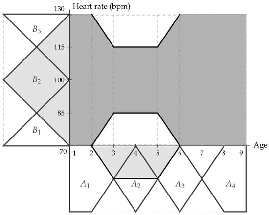
By performing an analogous process with the remaining elements of ${\mathcal{A}}_X$, we obtain the graphical representation in the $X\times Y$ plane of the greatest model ${\mathbf{M}}_{\Gamma }$, which corresponds to the shaded region in the $X\times Y$ plane shown in Figure 5. Note that the pairs $(x,y)\in X\times Y$ that lie on the “boundary” of the shaded section also belong to ${\mathbf{M}}_{\Gamma }$.

Figure 5. Graphical representation of the greatest model ${\mathbf{M}}_{\Gamma }$ in Example 3 (the shaded zone). Dashed lines represent the restrictions imposed by each rule in $\Gamma$ and solid lines are part of ${\mathbf{M}}_{\Gamma }$.

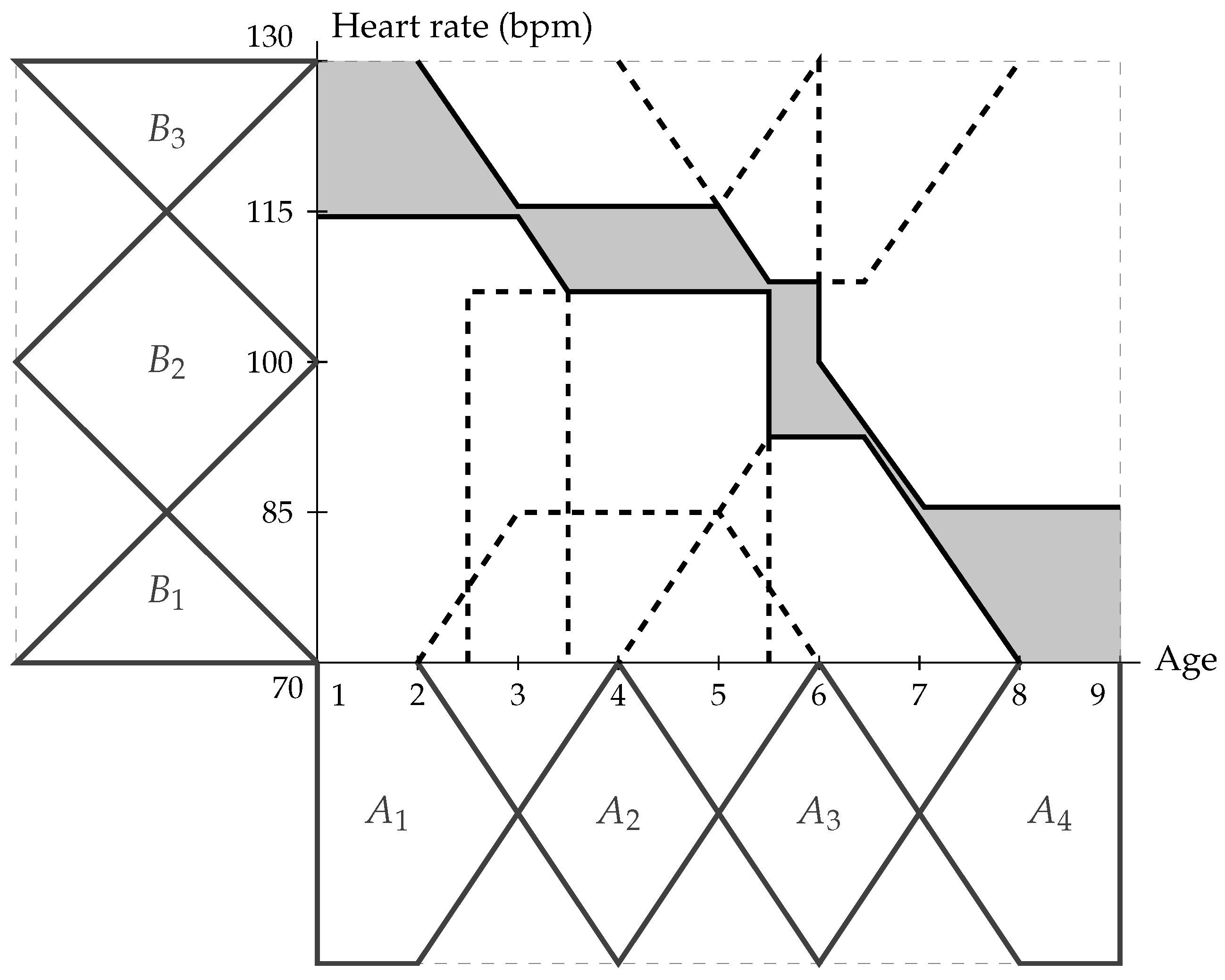
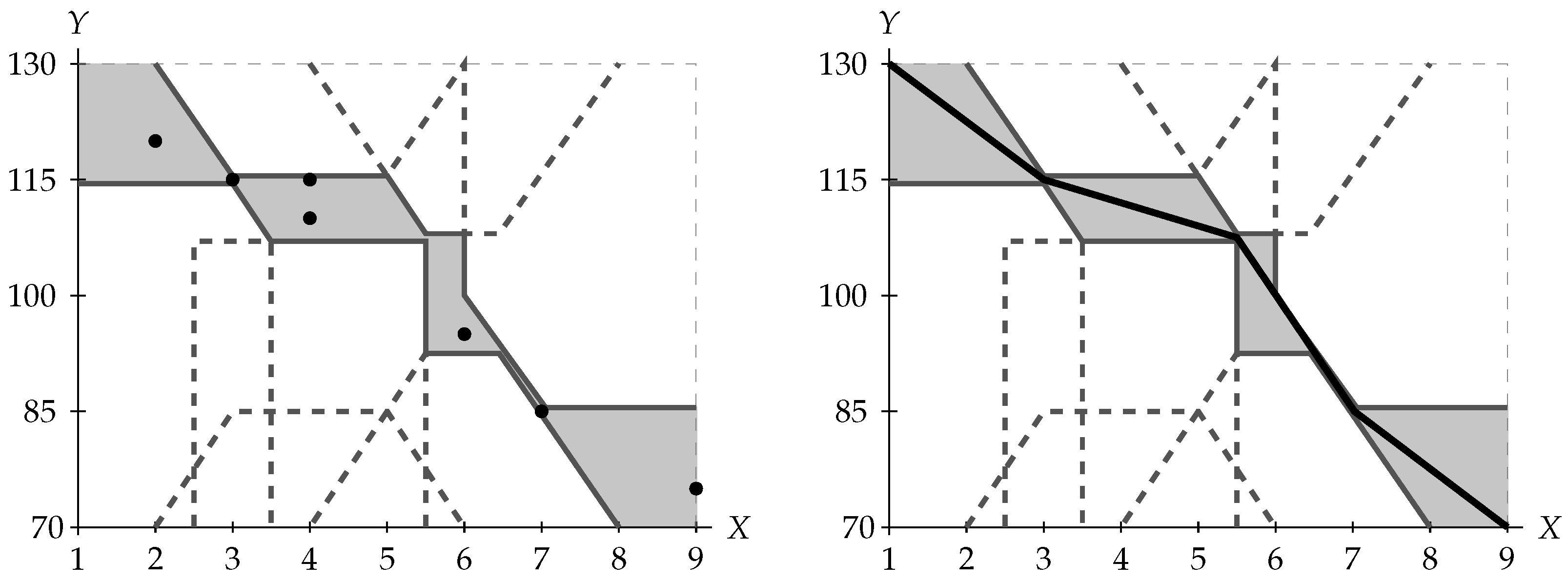
The computation of the greatest model provides an easy way to calculate other models of the $KB$, since the search for a model is reduced to selecting a set of pairs $(x,y)\in X\times Y$ that lie within the shaded region. In some applied environments, some models different from the greatest one may be of interest. For example, Figure 6 shows (in bold) two different models. The left graph presents a finite model, $M_1$, consisting of seven elements $(x,y)\in {\mathbf{M}}_{\Gamma }$:

$$M_1=\{(2,120),(3,115),(4,110),(4,115),(6,95),(7,85),(9,75)\}.$$

Figure 6. Left, graphical representation of the discrite model $M_1$ (with black dots) of $\Gamma$ in Example 3. Right, graphical representations of the functional model $M_2$ (with a black curve) of $\Gamma$ in Example 3. Dashed lines represent, in both graphs, the restrictions imposed by each rule in $KB$ and solid lines are part of ${\mathbf{M}}_{\Gamma }$.

On the other hand, the right graph in Figure 6 shows a model $M_2$ consisting of a functional dataset, namely, a set of pairs $(x,f\left(x\right))\in {\mathbf{M}}_{\Gamma }$.

The following result shows that with this semantics, we can identify each model of a $KB$ with one particular T-Box of the Description Logic ${\mathcal{LU}}_{FH}$ defined in the previous section. As shown in a subsequent section, this link allows the application of inference rules of ${\mathcal{LU}}_{FH}$ in our $KB$.

Proposition 3.

Let Γ be a $KB$ on a frame $(X,Y,{\mathcal{A}}_X,{\mathcal{B}}_Y)$, and let ${\mathbf{T}}_{\Gamma }$ be the T-Box of ${\mathcal{LU}}_{FH}$ constructed as follows:

• For each $A_i$ in ${\mathcal{A}}_X$ (resp., $B_j$ in ${\mathcal{B}}_Y$) consider the concept $C_{A_i}$ (resp., $C_{B_j}$);
• For each $f_{ij}\in \mathcal{G}$ appearing in Γ, consider the concept modifier $m_{ij}$;
• For each rule $⟨A_i\to B_j;f_{ij}⟩\in \Gamma$, consider in ${\mathbf{T}}_{\Gamma }$ the specialization concept

  $${}^{m_{ij}}C_{A_i}⊑C_{B_j}.$$

Then, given a model M of Γ, the interpretation $\mathcal{I}=({\Delta }_I,{·}^I)$ given by

• ${\Delta }^{\mathcal{I}}=M$;
• If $A_i\in {\mathcal{A}}_X$, then $C_{A_i}^{\mathcal{I}}(x,y)=A_i\left(x\right)$;
• If $B\in {\mathcal{B}}_Y$, then $C_{B_j}^{\mathcal{I}}(x,y)=B_j\left(y\right)$;
• ${{(}^{m_{ij}}C)}^{\mathcal{I}}(x,y)=f_{ij}\left(C^{\mathcal{I}}(x,y)\right)$;

is a model of ${\mathbf{T}}_{\Gamma }$.

Proof. 

Let $(x,y)\in M$. Then, by definition of a model, $f_{ij}\left(A_i\left(x\right)\right)\le B_j\left(y\right)$ for every rule in $\Gamma$, which implies that ${{(}^{m_{ij}}{C}_{A_i})}^{\mathcal{I}}(x,y))\le C_{B_j}^{\mathcal{I}}(x,y)$. In conclusion, $\mathcal{I}$ satisfies ${}^{m_{ij}}C_{A_i}⊑C_{B_j}$ for every concept specialization in ${\mathbf{T}}_{\Gamma }$. In other words, $\mathcal{I}$ is a model of ${\mathbf{T}}_{\Gamma }$. □

Obviously, the converse of the previous result is not true in general, since the models in ${\mathcal{LU}}_{FH}$ may be very general. Actually, a $KB$ with only empty models may be connected to a T-Box with non-empty models via the translation described in Proposition 3.

Example 4.

Let us consider, on the universes $X=\{x_1,x_2,x_3\}$ and $Y=\{y_1,y_2,y_3\}$, the fuzzy partitions ${\mathcal{A}}_X=\{A_1,A_2\}\subseteq \mathcal{F}\left(X\right)$ and ${\mathcal{B}}_Y=\{B_1,B_2\}\subseteq \mathcal{F}\left(Y\right)$ given by the fuzzy sets defined in Table 4.

Table 4. Membership functions of fuzzy sets in partitions ${\mathcal{A}}_X$ and ${\mathcal{B}}_Y$ in Example 4.

	${\mathit{x}}_1$	${\mathit{x}}_2$	${\mathit{x}}_3$			${\mathit{y}}_1$	${\mathit{y}}_2$	${\mathit{y}}_3$
$A_1$	1	1	0		$B_1$	1	$0.5$	0
$A_2$	0	0	1		$B_2$	0	$0.5$	1

On this frame $(X,Y,{\mathcal{A}}_X,{\mathcal{B}}_Y)$, we define the $KB$ composed by the next four rules:

• $⟨A_1\to B_1;id⟩$;    ● $⟨A_2\to B_1;{\displaystyle \frac{id}{2}}⟩$;
• $⟨A_1\to B_2;{\displaystyle \frac{id}{2}}⟩$;    ● $⟨A_2\to B_2;id⟩$.

Consider each element $(x_i,y_j)\in X\times Y$, and let us check that there is at least one rule in Γ that is not satisfied by $(x_i,y_i)$:

• $(x_1,y_1)$ and $(x_2,y_1)$ do not satisfy $⟨A_1\to B_2;{\displaystyle \frac{id}{2}}⟩$, since ${\displaystyle \frac{id}{2}}\left(A_1\left(x_1\right)\right)={\displaystyle \frac{id}{2}}\left(A_1\left(x_2\right)\right)=0.5\nleqq B_2\left(y_1\right)=0$.
• $(x_3,y_1)$ does not satisfy $⟨A_2\to B_2;id⟩$, because $A_2\left(x_3\right)=1\nleqq B_2\left(y_1\right)=0$.
• $(x_1,y_2)$ and $(x_2,y_2)$ do not satisfy $⟨A_1\to B_1;id⟩$, since $A_1\left(x_1\right)=A_1\left(x_2\right)=1\nleqq B_1\left(y_2\right)=0.5$.
• $(x_3,y_2)$ does not satisfy $⟨A_2\to B_2;id⟩$, because $A_2\left(x_3\right)=1\nleqq B_2\left(y_2\right)=0.5$.
• $(x_1,y_3)$ and $(x_2,y_3)$ do not satisfy $⟨A_1\to B_1;id⟩$, since $A_1\left(x_1\right)=A_1\left(x_2\right)=1\nleqq B_1\left(y_3\right)=0$.
• Finally, $(x_3,y_3)$ does not satisfy $⟨A_2\to B_1;{\displaystyle \frac{id}{2}}⟩$, since ${\displaystyle \frac{id}{2}}\left(A_2\left(x_3\right)\right)=0.5\nleqq B_1\left(y_3\right)=0$.

In conclusion, there is no pair $(x,y)\in X\times Y$ that belongs to a model of $KB$; in other words, the only model is the empty set, ${\mathbb{M}}_{\Gamma }=\{\varnothing \}$.

Now, let us define in ${\mathcal{LU}}_{FH}$ the set of concepts $\Pi =\{C_{A_1},C_{A_2},C_{B_1},C_{B_2}\}$ associated with each one of the elements of ${\mathcal{A}}_X$ and ${\mathcal{B}}_Y$, respectively, and consider the T-Box defined as in Proposition 3:

$${\mathbf{T}}_{\Gamma }=\left\{{⟨}^{m_1}{C}_{A_1}⊑C_{B_1}⟩,{⟨}^{m_2}{C}_{A_1}⊑C_{B_2}⟩,{⟨}^{m_2}{C}_{A_2}⊑C_{B_1}⟩,{⟨}^{m_1}{C}_{A_2}⊑C_{B_2}⟩\right\}.$$

Given the interpretation $\mathcal{I}=({\Delta }^{\mathcal{I}},{·}^{\mathcal{I}})$ where

• ${\Delta }^{\mathcal{I}}=\left\{u\right\}$;
• $C^{\mathcal{I}}\left(u\right)=0.5$ for all $u\in {\Delta }^{\mathcal{I}}$ and for every concept $C\in \Pi$;
• ${m_1}^{\mathcal{I}}=id$ and ${m_2}^{\mathcal{I}}={\displaystyle \frac{id}{2}}$;

it can be easily checked that $\mathcal{I}$ satisfies every concept specialization in ${\mathbf{T}}_{\Gamma }$. Therefore, $\mathcal{I}$ is a model of  ${\mathbf{T}}_{\Gamma }$.

4.2. Adding Inputs to $KB$s: Defining Consequences

In the previous subsection, we described the structure of $KB$; now, let us explain how to reason with it. The purpose of this fuzzy inference system is to draw conclusions from a $KB$ and a certain input. Let us begin by defining what is a $KB$-input on a frame.

Definition 17.

A $KB$-inputon the frame $(X,Y,{\mathcal{A}}_X,{\mathcal{B}}_Y)$ is a fuzzy set defined either on X or on Y.

Thanks to Proposition 3, it looks natural to incorporate inputs to $KB$s by giving a similar semantics to assertions in ${\mathcal{LU}}_{LH}$. Since assertions in ${\mathcal{LU}}_{LH}$ resemble the so-called $\alpha$-cuts in fuzzy set theory, our semantics considers $\alpha$-models that represent the $\alpha$-cuts of a (fuzzy) model.

Definition 18.

Let A (resp., B) be a $KB$-input on a frame $(X,Y,{\mathcal{A}}_X,{\mathcal{B}}_Y)$ such that $A\in \mathcal{F}\left(X\right)$ (resp., $B\in \mathcal{F}\left(Y\right)$), and let $\alpha \in [0,1]$. A subset of pairs $M\subseteq X\times Y$ is an $\alpha$-model of A (resp., B) if and only if $M\subseteq \left\{\right(x,y)\in X\times Y\mid A(x)\ge \alpha \}$ if and only if $M\subseteq \left\{\right(x,y)\in X\times Y\mid B(y)\ge \alpha \}$).

Under the previous definition of an $\alpha$-model, $KB$-inputs can be interpreted as constraints that bound the pairs of elements in $X\times Y$. Note that the greater the $KB$-input (as a fuzzy set), the weaker the restriction, since it admits more $\alpha$-models. On the other hand, the value $\alpha$ also determines a restriction in the sense that the greater the value $\alpha$, the stronger the restriction imposed to pairs in $X\times Y$ to be in an $\alpha$-model.

Note that from a theoretical point of view, we can assume theoretically that only two inputs can be considered: one fuzzy set on the universe X and another on Y. In other words, if we are interested in reasoning with two different fuzzy sets $A_1$ and $A_2$ on X, this is equivalent to considering the fuzzy set $A_1\cap A_2$ as a $KB$-input.

Proposition 4.

Let $A_1$ and $A_2$ be two $KB$-inputs on a frame $(X,Y,{\mathcal{A}}_X,{\mathcal{B}}_Y)$, both of them defined on the same universe. A subset of pairs $M\subseteq X\times Y$ is an α-model of $A_1$ and $A_2$ if and only if M is an α-model of $A_1\cap A_2$.

Proof. 

Let $A_1,A_2\in \mathcal{F}\left(X\right)$ and let M be an $\alpha$-model of $A_1$ and $A_2$. By definition of an $\alpha$-model, we have that for all $(x,y)\in M$, $A_1\left(x\right)\ge \alpha$ and $A_2\left(x\right)\ge \alpha$. That is equivalent to saying

$$A_1\cap A_2\left(x\right)=min\{A_1\left(x\right),A_2\left(x\right)\}\ge \alpha .$$

Therefore, M is a model of $A_1\cap A_2$. □

As a consequence of the previous result, we can combine different fuzzy sets defined on the same universe into one $KB$-input and keep the semantics. Thus, as mentioned before, from a theoretical point of view, only two inputs are possible, one fuzzy set on the universe X and another on the universe Y. For the sake of simplicity in this approach, we only consider one $KB$-input for reasoning.

The following result shows that the set of $\alpha$-models has a complete lattice structure.

Proposition 5.

Let A be a $KB$-input on a frame $(X,Y,{\mathcal{A}}_X,{\mathcal{B}}_Y)$. Fixing $\alpha \in [0,1]$, the set of α-models of A has the structure of a complete lattice.

It is also convenient for the reader to keep the following meaning of a $KB$-input A: the fuzzy set A determines the set of possible values of X (or Y) a system may consider for reasoning with. In this way, we focus on determining the greater set of possible values in $X\times Y$ that satisfy the constraints represented by the rules in both a $KB$ and in a $KB$-input. The following definition determines the semantics for the fusion of the knowledge represented by a $KB$ and the restriction imposed by a $KB$-input as a fuzzy set on $X\times Y$.

Definition 19.

Let Γ be a $KB$, and let A be a $KB$-input on a frame $(X,Y,{\mathcal{A}}_X,{\mathcal{B}}_Y)$. A model of $\Gamma \cup \left\{A\right\}$ is a fuzzy set M on the universe $X\times Y$ such that for each $\alpha >0$, the α-cut $M^{\alpha }=\{(x,y)\in X\times Y\mid M(x,y)\ge \alpha \}$ is a model of Γ and an α-model of A.

Note that a model of the pair of a $KB$ $\Gamma$ and a $KB$-input A is a fuzzy set constructed by $\alpha$-cuts that intersect models of $\Gamma$ and $\alpha$-models of A. The following result shows an equivalent definition of a model that is used in some proofs of further results.

Theorem 6.

Let Γ be a $KB$, and let A be a $KB$-input on a frame $(X,Y,{\mathcal{A}}_X,{\mathcal{B}}_Y)$. M is a model of $\Gamma \cup \left\{A\right\}$ if and only if $supp\left(M\right)$ is a model of Γ and $M(x,y)\le A\left(x\right)$.

Proof. 

Let us start by proving the backward implication, as it is more straightforward:

⇐

Let $M\in \mathcal{F}(X\times Y)$, and let us assume that $supp\left(M\right)$ is a model of $\Gamma$ and that $M(x,y)\le A\left(x\right)$ for all $(x,y)\in X\times Y$. Let us prove that M is a model of $\Gamma \cup \left\{A\right\}$. Consider the $\alpha$-cut $M^{\alpha }$ with fixed $\alpha >0$:

–

First, since $M^{\alpha }\subseteq supp\left(M\right)=\{(x,y)\in X\times Y\mid M(x,y)>0\}$ and $supp\left(M\right)$ is a model of $\Gamma$, $M^{\alpha }$ is also a model of $\Gamma$.

–

Second, for each $(x,y)\in M^{\alpha }$, we have that $\alpha \le M(x,y)\le A\left(x\right)$ by assumption. Then, $\alpha \le A\left(x\right)$ for all $(x,y)\in M^{\alpha }$. In consequence, $M^{\alpha }\subseteq \{(x,y)\in X\times Y\mid A\left(x\right)\ge \alpha \}$, namely, $M^{\alpha }$ is an $\alpha$-model of A.

⇒

Assume that $M\in \mathcal{F}(X\times Y)$ is a model of $\Gamma \cup \left\{A\right\}$. Then,

–

On the one hand, by Definition 19, every $M^{\alpha }$ with $\alpha >0$ is a model of $\Gamma$. Moreover, the support of a fuzzy set can be characterized by

$$supp\left(M\right)=\bigcup _{\alpha >0}{M}^{\alpha }.$$

Since, by Theorem 5, $({\mathbb{M}}_{\Gamma },\subseteq )$ is a complete lattice, $supp\left(M\right)$ is also a model of $\Gamma$.

–

On the other hand, by Definitions 18 and 19, every $M^{\alpha }$ with $\alpha >0$ is also an $\alpha$-model of A, which means that $M^{\alpha }\subseteq \{(x,y)\in X\times Y\mid A\left(x\right)\ge \alpha \}$. Let us prove by reductio ad absurdum that $M(x,y)\le A\left(x\right)$ for all $(x,y)\in X\times Y$. Suppose that there exists an element $(x_0,y_0)\in X\times Y$ such that

$$\beta =M(x_0,y_0)>A\left(x_0\right)$$

for certain $\beta \in (0,1]$. Then, by definition, $(x_0,y_0)$ belongs to the $\beta$-cut of M, i.e., $\beta \in M^{\beta }$. By assumption, $M^{\beta }$ is a $\beta$-model of A, which implies

$$(x_0,y_0)\in M^{\beta }\subseteq \{(x,y)\in X\times Y\mid A\left(x\right)\ge \beta \}$$

which implies that $A\left(x_0\right)\ge \beta$. This leads us to a contradiction since

$$\beta \le A\left(x_0\right)<M(x_0,y_0)=\beta$$

which completes the proof.

□

In Theorem 5, it was already demonstrated that for every $KB$, there exists a greatest model associated with it. The following theorem presents an analogous result for models $KB$s with $KB$-inputs.

Theorem 7.

Let Γ be a $KB$, and let A be a $KB$-input on a frame $(X,Y,{\mathcal{A}}_X,{\mathcal{B}}_Y)$. The set of models of $\Gamma \cup \left\{A\right\}$, denoted by ${\mathbb{M}}_{\Gamma ,A}$, has a complete lattice structure with the standard Zadeh’s ordering between fuzzy sets (i.e., $A\le B$ if and only if $A\left(x\right)\le B\left(x\right))$.

Proof. 

Let us begin by proving that ${\mathbb{M}}_{\Gamma ,A}$ is closed by the union of arbitrary models. Let ${\left\{M_i\right\}}_{i\in I}\in {\mathbb{M}}_{\Gamma ,A}$, and let us show that both fuzzy sets ${\mathbf{M}}_{\cup }={\bigcup }_{i\in I}{M}_i$ and ${\mathbf{M}}_{\cap }={\bigcap }_{i\in I}{M}_i$ are models of $\Gamma \cup \left\{A\right\}$, i.e., they are in ${\mathbb{M}}_{\Gamma ,A}$. By Theorem 6:

• We know that $M_i(x,y)\le A\left(x\right)$ for all $i\in I$ and $(x,y)\in X\times Y$;
• The result is reduced to prove that prove that ${\mathbf{M}}_{\cup }(x,y)\le A\left(x\right)$ and ${\mathbf{M}}_{\cap }(x,y)\le A\left(x\right)$ for all $(x,y)\in X\times Y$.

Let $(x,y)\in X\times Y$; then,

$$\begin{array}{cc}\hfill {\mathbf{M}}_{\cup }(x,y)& =\underset{i\in I}{sup}{M}_i(x,y)\le A\left(x\right);\hfill \\ \hfill {\mathbf{M}}_{\cap }(x,y)& =\underset{i\in I}{inf}{M}_i(x,y)\le A\left(x\right).\hfill \end{array}$$

This is what we wanted to prove. □

It it straightforward to check that the empty set is the least model of ${\mathbb{M}}_{\Gamma ,A}$. The following theorem shows the expression of the greatest model of ${\mathbb{M}}_{\Gamma ,A}$.

Theorem 8.

Let Γ be a $KB$ and A be a $KB$-input on a frame $(X,Y,{\mathcal{A}}_X,{\mathcal{B}}_Y)$. The greatest model of $\Gamma \cup \left\{A\right\}$, denoted by ${\mathbf{M}}_{\Gamma ,\mathbf{A}}$, is the fuzzy set given by the restriction of the support of A to the greatest model of  Γ:

$${\mathbf{M}}_{\Gamma ,\mathbf{A}}(x,y)=\left\{\begin{array}{cc}A\left(x\right)& \hfill \mathit{if}(x,y)\in {\mathbf{M}}_{\Gamma }\\ 0& \hfill \mathit{otherwise}.\end{array}\right.$$

(2)

Proof. 

Let us prove that ${\mathbf{M}}_{\Gamma ,\mathbf{A}}$ is a model of $\Gamma \cup \left\{A\right\}$ and that every model M of $\Gamma \cup \left\{A\right\}$ satisfies $M\le {\mathbf{M}}_{\Gamma ,\mathbf{A}}$. Then, necessarily, ${\mathbf{M}}_{\Gamma ,\mathbf{A}}$ is the greatest model of $\Gamma \cup \left\{A\right\}$.

By Theorem 6, ${\mathbf{M}}_{\Gamma ,\mathbf{A}}$ is a model of $\Gamma \cup \left\{A\right\}$, since by definition, ${\mathbf{M}}_{\Gamma ,\mathbf{A}}(x,y)\le A\left(x\right)$ for all $(x,y)\in X\times Y$.

On the other hand, let M be a model of ${\mathbf{M}}_{\Gamma ,\mathbf{A}}$ and let us assume by reductio ad absurdum that there exists $(x_0,y_0)\in X\times Y$ such that $M(x_0,y_0)>{\mathbf{M}}_{\Gamma ,\mathbf{A}}(x_0,y_0)$. By definition, we have that $M(x_0,y_0)>{\mathbf{M}}_{\Gamma ,\mathbf{A}}(x_0,y_0)=A\left(x_0\right)$, which contradicts the fact that M is a model according to the characterization of Theorem 6. □

We can now introduce the notion of logical consequence as usual in formal logic theories.

Definition 20.

Let Γ be a $KB$, and let A be a $KB$-input on a frame $(X,Y,{\mathcal{A}}_X,{\mathcal{B}}_Y)$. We say that a fuzzy set $B\in \mathcal{F}\left(X\right)$ (resp., $B\in \mathcal{F}\left(Y\right)$) is a consequence of $\Gamma \cup \left\{A\right\}$, denoted by $\Gamma \cup \left\{A\right\}\vDash B$, if for every model M of $\Gamma \cup \left\{A\right\}$, we have $B\left(x\right)\ge M(x,y)$ for all $(x,y)\in X\times Y$ (resp., $B\left(y\right)\ge M(x,y)$ for all $(x,y)\in X\times Y$).

Thanks to the complete lattice structure of the set of models of $\Gamma \cup \left\{A\right\}$ (see Theorem 7), we can reduce the validation of consequences to checking the greatest model of $\Gamma \cup \left\{A\right\}$.

Theorem 9.

Let Γ be a $KB$, and let A be a $KB$-input on a frame $(X,Y,{\mathcal{A}}_X,{\mathcal{B}}_Y)$. A fuzzy set $B\in \mathcal{F}\left(X\right)$ (resp., $B\in \mathcal{F}\left(Y\right)$) is a consequence of $\Gamma \cup \left\{A\right\}$ if and only if we have $B\left(x\right)\ge {\mathbf{M}}_{\Gamma ,\mathbf{A}}(x,y)$ for all $(x,y)\in X\times Y$ (resp., $B\left(y\right)\ge {\mathbf{M}}_{\Gamma ,\mathbf{A}}(x,y)$), where ${\mathbf{M}}_{\Gamma ,\mathbf{A}}$ is the greatest model of $\Gamma \cup \left\{A\right\}$.

Proof. 

Suppose that $B\in \mathcal{F}\left(X\right)$ (the proof for the case $B\in \mathcal{F}\left(Y\right)$ is similar) and that $\Gamma \cup \left\{A\right\}\vDash B$. Then, every model M of $\Gamma \cup \left\{A\right\}$ satisfies $B\left(x\right)\ge M(x,y)$ for all $(x,y)\in X\times Y$. In particular, that inequality holds for the greatest model ${\mathbf{M}}_{\Gamma ,\mathbf{A}}$. That is, $B\left(x\right)\ge {\mathbf{M}}_{\Gamma ,\mathbf{A}}(x,y)$ for all $(x,y)\in X\times Y$.

Conversely, let us assume that $B\left(y\right)\ge {\mathbf{M}}_{\Gamma ,\mathbf{A}}(x,y)$ for all $(x,y)\in X\times Y$. Given a model M of $\Gamma \cup \left\{A\right\}$, we have that $M(x,y)\le {\mathbf{M}}_{\Gamma ,\mathbf{A}}(x,y)$ for all $(x,y)\in X\times Y$, since ${\mathbf{M}}_{\Gamma ,\mathbf{A}}$ is the greatest model of $({\mathbb{M}}_{\Gamma ,A},\le )$. Therefore,

$$B\left(y\right)\ge {\mathbf{M}}_{\Gamma ,\mathbf{A}}(x,y)\ge M(x,y)$$

for all $(x,y)\in X\times Y$ and $\Gamma \cup \left\{A\right\}\vDash B$. □

From the previous characterization, it is obvious that in order to determine consequences, we can focus only on the greatest model of $\Gamma \cup \left\{A\right\}$. The following result shows that when considering a $KB$ with a simple condition of coherence, determining whether a fuzzy set defined on the same universe as the $KB$-input is a consequence is trivial.

Theorem 10.

Let Γ be a $KB$ on a frame $(X,Y,{\mathcal{A}}_X,{\mathcal{B}}_Y)$. Let us assume that for each $x\in X$ and $y\in Y$, there exists $y_x\in Y$ and $x_y\in X$ such that $\{(x,y_x),(x_y,y)\}$ is a model of Γ. Then:

• Given $A,B\in \mathcal{F}\left(X\right)$, $\Gamma \cup \left\{A\right\}\vDash B$ if and only if $A\le B$;
• Given $A,B\in \mathcal{F}\left(Y\right)$, $\Gamma \cup \left\{A\right\}\vDash B$ if and only if $A\le B$.

Proof. 

Let us prove the first item, since the second is proved similarly. Let ${\mathbf{M}}_{\Gamma ,\mathbf{A}}$ be the greatest model of $\Gamma \cup \left\{A\right\}$. From Theorem 8, we have that ${\mathbf{M}}_{\Gamma ,\mathbf{A}}(x,y)=A\left(x\right)$ for all $(x,y)\in {\mathbf{M}}_{\Gamma }$ and ${\mathbf{M}}_{\Gamma ,\mathbf{A}}(x,y)=0$ if $(x,y)\notin {\mathbf{M}}_{\Gamma }$. Let $B\in \mathcal{F}\left(X\right)$ such that $\Gamma \cup \left\{A\right\}\vDash B$. Then, by Theorem 9, that is equivalent to say that ${\mathbf{M}}_{\Gamma ,\mathbf{A}}(x,y)\le B\left(x\right)$. Then, for each $x\in X$, and choosing $y_x\in Y$ such that $(x,y_x)\in {\mathbf{M}}_{\Gamma }$, we have

$$A\left(x\right)={\mathbf{M}}_{\Gamma ,\mathbf{A}}(x,y_x)\le B\left(x\right),$$

which is equivalent to say that $A\le B$. □

From the previous result we have the following: given a $KB$ $\Gamma$ on a frame $(X,Y,{\mathcal{A}}_X,{\mathcal{B}}_Y)$ and a $KB$-input $A\in \mathcal{F}\left(X\right)$, the only non-trivial consequences of $\Gamma \cup \left\{A\right\}$ are those fuzzy sets defined on Y. The following proposition shows that there is a monotonicity on the set of consequences with respect to the ordering of fuzzy sets with respect to Zadeh’s ordering.

Proposition 6.

Let Γ be a $KB$ and $A\in \mathcal{F}\left(X\right)$ be a $KB$-input on a frame $(X,Y,{\mathcal{A}}_X,{\mathcal{B}}_Y)$. Let $B,C\in \mathcal{F}\left(Y\right)$ such that $B\subseteq C$ and $\Gamma \cup \left\{A\right\}\vDash B$; then, $\Gamma \cup \left\{A\right\}\vDash C$.

Proof. 

Consider a model M of $\Gamma \cup \left\{A\right\}$. If $\Gamma \cup \left\{A\right\}\vDash B$, then (Theorem 9) $B\left(y\right)\ge M(x,y)$ for all $(x,y)\in X\times Y$. Since $B\left(y\right)\le C\left(y\right)$ for all $y\in Y$, then $C\left(y\right)\ge M(x,y)$ for all $(x,y)\in X\times Y$. Again, by Theorem 9, we can conclude that $\Gamma \cup \left\{A\right\}\vDash C$. □

It can be also proved that the set of consequences of $\Gamma \cup \left\{A\right\}$ inherits the complete lattice structure from the set of models of $\Gamma \cup \left\{A\right\}$.

Proposition 7.

Let Γ be a $KB$ and $A\in \mathcal{F}\left(X\right)$ be a $KB$-input on a frame $(X,Y,{\mathcal{A}}_X,{\mathcal{B}}_Y)$. The set of consequences of $\Gamma \cup \left\{A\right\}$, i.e., the set $\{B\in \mathcal{F}(Y)\mid \Gamma \cup \{A\}\vDash B\}$, has a complete lattice structure with greatest element Y.

Proof. 

Let $\mathcal{C}$ be the set of consequences of $\Gamma \cup \left\{A\right\}$, and let ${\left\{B_i\right\}}_{i\in I}\subseteq \mathcal{C}$. By Proposition 6, we have directly that ${\bigcup }_{i\in I}{B}_i$ is a consequence of $\Gamma \cup \left\{A\right\}$.

Let us prove now that ${\bigcap }_{i\in I}{B}_i$ is a consequence of $\Gamma \cup \left\{A\right\}$ as well. By definition of a consequence, we have that for all $B_i$’s and all models M of $\Gamma \cup \left\{A\right\}$, we have $B_i\left(y\right)\ge M(x,y)$ for all $(x,y)\in X\times Y$. As a result,

$$\bigcap _{i\in I}{B}_i\left(y\right)\ge M(x,y)$$

for all models M and all $(x,y)\in X\times Y$. That is, ${\bigcap }_{i\in I}{B}_i$ is a consequence of $\Gamma \cup \left\{A\right\}$. □

Corollary 2.

Let Γ be a $KB$ and $A\in \mathcal{F}\left(X\right)$ be a $KB$-input on a frame $(X,Y,{\mathcal{A}}_X,{\mathcal{B}}_Y)$. Let $B,C\in \mathcal{F}\left(Y\right)$ be two fuzzy sets such that $\Gamma \cup \left\{A\right\}\vDash B$ and $\Gamma \cup \left\{A\right\}\vDash C$; then,

• $\Gamma \cup \left\{A\right\}\vDash B\cap C$;
• $\Gamma \cup \left\{A\right\}\vDash B\cup C$.

4.3. Inference Engine: Links with ${\mathcal{LU}}_{FH}$

In the previous section, we showed that given a $KB$ $\Gamma$ and a $KB$-input $A\in \mathcal{F}\left(X\right)$, the set of consequences was determined by the greatest model of $\Gamma \cup \left\{A\right\}$ or by the least consequence on $\mathcal{F}\left(Y\right)$. Determining the greatest model and checking whether a fuzzy set is a consequence by comparison with it may be complex from a computational point of view. In this section, we propose a simple inference process to obtain correct consequences that upper-bound the least consequence of $\Gamma \cup \left\{A\right\}$.

In order to keep the support of our fuzzy inference system on the Description Logic ${\mathcal{LU}}_{FH}$ (and its power of reasoning), it would be desirable to link the models of both constructions, as linked in the previous section by Proposition 3. The following theorem presents an analogous result for a $KB$ and a $KB$-input by fixing elements in $\alpha$-cuts of models.

Theorem 11.

Let Γ be a $KB$ and let $A\in \mathcal{F}\left(X\right)$ be a $KB$-input on a frame $(X,Y,{\mathcal{A}}_X,{\mathcal{B}}_Y)$. Let ${\mathbf{A}}_{\Gamma }$ be the A-Box of ${\mathcal{LU}}_{FH}$ constructed as follows:

• For each $A_i$ in ${\mathcal{A}}_X$, consider the concept $C_{A_i}$;
• For A in $\mathcal{F}\left(X\right)$, consider the concept $C_A$;
• For each concept $C_{A_i}$, consider the pair of concept modifiers $⟨m_i,{\overline{m}}_i⟩$;
• For each concept $C_{A_i}$, consider in ${\mathbf{A}}_{\Gamma }$ the assertion

  $${⟨}^{{\overline{m}}_i}{C}_{A_i}\left(a\right)\alpha ⟩,$$
  where $\alpha \in (0,1]$.

Consider a non-empty model M of $\Gamma \cup \left\{A\right\}$, its α-cut $M^{\alpha }$, and $(x_0,y_0)\in M^{\alpha }$. Then, the interpretation $\mathcal{I}=(M^{\alpha },{·}^{\mathcal{I}})$ given in Proposition 3 plus

• $a^{\mathcal{I}}=(x_0,y_0)$ and
• $m_i^{\mathcal{I}}={Inc}_{\mathcal{G}}(A,A_i)$

is a model of ${\mathbf{A}}_{\Gamma }$.

Proof. 

By definition of the f-index of inclusion,

$${Inc}_{\mathcal{G}}(A,A_i)\left(A\left(x\right)\right)\le A_i\left(x\right)$$

for all $A_i\in \mathcal{F}\left(X\right)$ and for every element $(x,y)$ of $M^{\alpha }$. Then, the interpretation $\mathcal{I}=(M^{\alpha },{·}^{\mathcal{I}})$ satisfies

$$m_i^{\mathcal{I}}\left(C_A^{\mathcal{I}}(x,y)\right)\le C_{A_i}^{\mathcal{I}}(x,y)$$

for all $(x,y)\in M^{\alpha }$. In other words, it satisfies the concept specialization ${}^{m_i}C_A⊑C_{A_i}$. Then, by Theorem 2, $\mathcal{I}$ must also satisfy $C_A⊑{}^{{\overline{m}}_i}C_{A_i}$.

At the same time, since the instance a of $C_{Ai}$ satisfies $a^{\mathcal{I}}=(x_0,y_0)\in M^{\alpha }$ and $M^{\alpha }$ is an $\alpha$-model of A, $C_A^{\mathcal{I}}\left(a^{\mathcal{I}}\right)=A\left(x_0\right)\ge \alpha$. Therefore, given the assertion ${⟨}^{{\overline{m}}_i}{C}_{A_i}\left(a\right),\alpha ⟩$:

$$\alpha \le C_A^{\mathcal{I}}\left(a^{\mathcal{I}}\right)\le {\overline{m}}_i^{\mathcal{I}}\left(C_{A_i}^{\mathcal{I}}\left(a^{\mathcal{I}}\right)\right).$$

In conclusion, $\mathcal{I}$ satisfies the assertion ${⟨}^{{\overline{m}}_i}{C}_{A_i}\left(a\right),\alpha ⟩$ for all $A_i\in {\mathcal{A}}_X$, and therefore, $\mathcal{I}$ is a model of ${\mathbf{A}}_{\Gamma }$. □

Note that $KB$-inputs $A\in \mathcal{F}\left(X\right)$ in a $KB$ and a frame $(X,Y,{\mathcal{A}}_X,{\mathcal{B}}_Y)$ are translated as a series of assertions in Description Logic through concept modifiers ${Inc}_{\mathcal{G}}(A,A_i)$ for each one of the elements of the partition $A_i\in {\mathcal{A}}_X$. That is to say, for each $KB$-input, $A\in \mathcal{F}\left(X\right)$ is considered an A-Box consisting of as many assertions as there are elements in the partition ${\mathcal{A}}_X$. This identification is carried out individually for each pair $(x,y)$ in the support of the model $M\in {\mathbb{M}}_{\Gamma ,A}$, taking into account the $\alpha$-cuts of M due to the specific characteristics of Description Logic, i.e., DL only allows for the inclusion of a countable set of instances, whereas the universes X and Y can be of a fundamentally different nature, such as $\mathbb{R}$. However, this identification of the instance a (in ${\mathcal{LU}}_{FH}$) with its corresponding $(x,y)$ is fixed but arbitrary within the $\alpha$-cut $M^{\alpha }$, as is the choice of the value $\alpha \in (0,1]$. This makes it possible to translate the assertions $⟨C_A\left(a\right),\alpha ⟩$ defined in ${\mathcal{LU}}_{FH}$ into a fuzzy set A defined on a universe X or Y.

The next result justifies the use of reasoning tools from Description Logic within our framework, and in particular, the application of the Generalized Modus Ponens given in Theorem 4.

Corollary 3.

Let Γ be a $KB$ and let A be a $KB$-input on a frame $(X,Y,{\mathcal{A}}_X,{\mathcal{B}}_Y)$. Let ${\mathbf{T}}_{\Gamma }$ be the T-Box of ${\mathcal{LU}}_{FH}$ and ${\mathbf{A}}_{\Gamma }$ the A-Box of ${\mathcal{LU}}_{FH}$ constructed as in Proposition 3 and Theorem 11, respectively. Then, all fuzzy assertions entailed by the set of axioms $⟨{\mathbf{T}}_{\Gamma },{\mathbf{A}}_{\Gamma }⟩$ (on the context of ${\mathcal{LU}}_{FH}$) form a correct inference from Γ and A (interpreted as $KB$ and $KB$-input).

Proof. 

Let $⟨C\left(a\right),\beta ⟩$ be a fuzzy assertion entailed by $⟨{\mathbf{T}}_{\Gamma },{\mathbf{A}}_{\Gamma }⟩$, which means that every model of $⟨{\mathbf{T}}_{\Gamma },{\mathbf{A}}_{\Gamma }⟩$ satisfies $⟨C\left(a\right),\beta ⟩$ as well. Then, given a model M of $\Gamma \cup \left\{A\right\}$ and given the interpretation $\mathcal{I}=(M^{\alpha },{·}^{\mathcal{I}})$, with $\alpha \in (0,1]$, defined in Proposition 3 and Theorem 11, it is guaranteed that $\mathcal{I}$ is a model of $⟨{\mathbf{T}}_{\Gamma },{\mathbf{A}}_{\Gamma }⟩$; therefore, it also satisfies $⟨C\left(a\right),\beta ⟩$. As $C^{\mathcal{I}}\left(a^{\mathcal{I}}\right)\ge \beta$ and $a^{\mathcal{I}}\in M^{\alpha }$, it can be concluded that $M^{\alpha }$ is a $\beta$-model of $C^{\mathcal{I}}$. □

As a consequence of the previous corollary, we can apply tools of inference from the Description Logic ${\mathcal{LU}}_{FH}$ on $KB$ and $KB$-inputs. Among all of them, we are interested here on the Generalized Modus Ponens (GMP) described on Section 3.3. Specifically, we can join all the possible GMP applicable on the T-Box and A-Box constructed according to Proposition 3 and Theorem 11 and obtain the following inference on $KB$, which is the core of the inference engine considered in our approach.

Theorem 12.

Let Γ be a $KB$ and let A be a $KB$-input on a frame $(X,Y,{\mathcal{A}}_X,{\mathcal{B}}_Y)$, where $A\in \mathcal{F}\left(X\right)$. Then, for all $⟨A_i\to B_j;f_{ij}⟩\in \Gamma$, we have

$$\{⟨A_i\to B_j;f_{ij}⟩,A\}\vDash B_{ij},$$

where $B_{ij}\in \mathcal{F}\left(Y\right)$ is the fuzzy set given by

$$B_{ij}\left(y\right)={\overline{\mathrm{Inc}}}_{\mathcal{G}}(A,A_i)\circ {\overline{f}}_{ij}\left(B_j\left(y\right)\right),$$

(3)

where ${\overline{f}}_{ij}$ is the only mapping such that $(f_{ij},{\overline{f}}_{ij})$ forms an adjoint pair.

Proof. 

Consider in ${\mathcal{LU}}_{FH}$ the T-Box ${\mathbf{T}}_{\Gamma }$ and the A-Box ${\mathbf{A}}_{\Gamma }$ constructed as in Proposition 3 and Theorem 11, respectively, by a fixed model M of $\Gamma \cup \left\{A\right\}$ and a fixed $\alpha$-cut of M, $M^{\alpha }$, with $\alpha \in (0,1]$. Given the construction of both sets, one can rearrange them in pairs of elements $\left(⟨{}^{m_{ij}}C_{A_i}⊑C_{B_j}⟩,⟨{}^{{\overline{m}}_i}C_{A_i}\left(a\right),\alpha ⟩\right)\in {\mathbf{T}}_{\Gamma }\times {\mathbf{A}}_{\Gamma }$ related through the concept specialization antecedent $C_{A_i}$. Then, by applying the Generalized Modus Ponens given in Theorem 4, we have

$$⟨{}^{m_{ij}}C_{A_i}⊑C_{B_j}⟩,⟨{}^{{\overline{m}}_i}C_{A_i}\left(a\right),\alpha ⟩\vDash ⟨{}^{{\overline{m}}_i\circ {\overline{m}}_{ij}}C_{B_{ij}}\left(a\right),\alpha ⟩,$$

where the concept ${}^{{\overline{m}}_i\circ {\overline{m}}_{ij}}C_{B_{ij}}$ obtained as an output is interpreted as

$${{(}^{{\overline{m}}_i\circ {\overline{m}}_{ij}}{C}_{B_{ij}})}^{\mathcal{I}}(x,y)={\overline{\mathrm{Inc}}}_{\mathcal{G}}(A,A_i)\circ {\overline{f}}_{ij}\left(B_j\left(y\right)\right)$$

for all $(x,y)\in M$. If we denote this fuzzy set as $B_{ij}$, it is concluded that $M^{\alpha }$ is an $\alpha$-model of $B_{ij}$. □

The previous result leads to the application of the following inference engine for a frame $(X,Y,{\mathcal{A}}_X,{\mathcal{B}}_Y)$ and a $KB$. Given a $KB$-input $A\in \mathcal{F}\left(X\right)$, for each pair $(A_i,B_j)\in {\mathcal{A}}_X\times {\mathcal{B}}_Y$, there exists a rule $⟨A_i\to B_j;f_{ij}⟩$ from which we can obtain the following inference:

$$B_{ij}\left(y\right)={\overline{\mathrm{Inc}}}_{\mathcal{G}}(A,A_i)\circ {\overline{f}}_{ij}\left(B_j\left(y\right)\right)\in \mathcal{F}\left(Y\right),$$

where $\overline{f}$ is the only mapping such that $(f,\overline{f})$ is an adjoint pair, as is ${\overline{\mathrm{Inc}}}_{\mathcal{G}}(A,A_i)$ with respect to ${Inc}_{\mathcal{G}}(A,A_i)$, i.e., the f-index of inclusion of A into $A_i$ is restricted to the set $\mathcal{G}$ (Definition 6).

Thanks to Theorem 12, we obtain the consequence $\Gamma \cup \left\{A\right\}\vDash B_{ij}$ for each pair $(A_i,B_j)\in {\mathcal{A}}_X\times {\mathcal{B}}_Y$, where ${\mathcal{A}}_X={\left\{A_i\right\}}_{i\in I}$ and ${\mathcal{B}}_Y={\left\{B_j\right\}}_{j\in J}$. By Corollary 2, we can conclude that the intersections and unions of the $B_{ij}$ are also consequences. Since our goal is to find the smallest set that is a consequence of $\Gamma$ and A, the inference engine takes the infimum of all of them. This leads to our inference engine:

$$B\left(y\right)=\left(\bigcap _{\begin{array}{c}i\in I,\\ j\in J\end{array}}{B}_{ij}\right)\left(y\right)=\underset{\begin{array}{c}{A}_i\in {\mathcal{A}}_X,\\ B_j\in {\mathcal{B}}_Y\end{array}}{inf}{\overline{\mathrm{Inc}}}_{\mathcal{G}}(A,A_i)\circ {\overline{f}}_{ij}\left(B_j\left(y\right)\right),$$

(4)

which is called the $KB$-output of $\Gamma \cup \left\{A\right\}$. The next result states that the fuzzy set obtained by our inference engine is actually a consequence of a $KB$ and a $KB$-input.

Corollary 4.

Let Γ be a $KB$ and let $A\in \mathcal{F}\left(X\right)$ be a $KB$-input on a frame $(X,Y,{\mathcal{A}}_X,{\mathcal{B}}_Y)$. Then, the fuzzy set $B\in \mathcal{F}\left(Y\right)$ defined by Equation (4) is a consequence of $\Gamma \cup \left\{A\right\}$, that is, $\Gamma \cup \left\{A\right\}\vDash B$.

Proof. 

As a consequence of Theorem 12, given a model of $\Gamma \cup \left\{A\right\}$, every $\alpha$-model of A with $\alpha \in (0,1]$ is also an $\alpha$-model if $B_{ij}$, which means that every $(x,y)\in M^{\alpha }$ satisfies $B_{ij}\left(y\right)\ge \alpha$. Then, the fuzzy set defined in Equation (4) also satisfies

$$B\left(y\right)=\left(\bigcap _{\begin{array}{c}i\in I,\\ j\in J\end{array}}{B}_{ij}\right)\left(y\right)=\underset{\begin{array}{c}i\in I,\\ j\in J\end{array}}{inf}{B}_{ij}\left(y\right)\ge \alpha$$

for every $(x,y)\in M^{\alpha }$. In consequence, $M^{\alpha }$ is an $\alpha$-model of the $KB$-output B. □

Let us look at a pair of examples applying this inference engine to the $KB$ defined previously in Example 3. First, we study the case where the $KB$-input introduced is a singleton. Second, the case where the $KB$-input is a more general fuzzy set is studied.

Example 5.

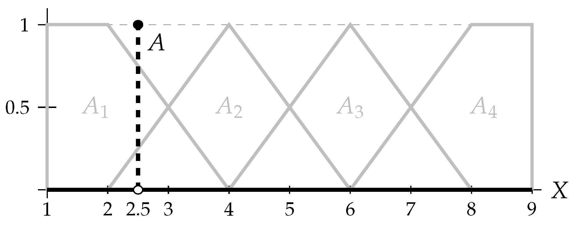
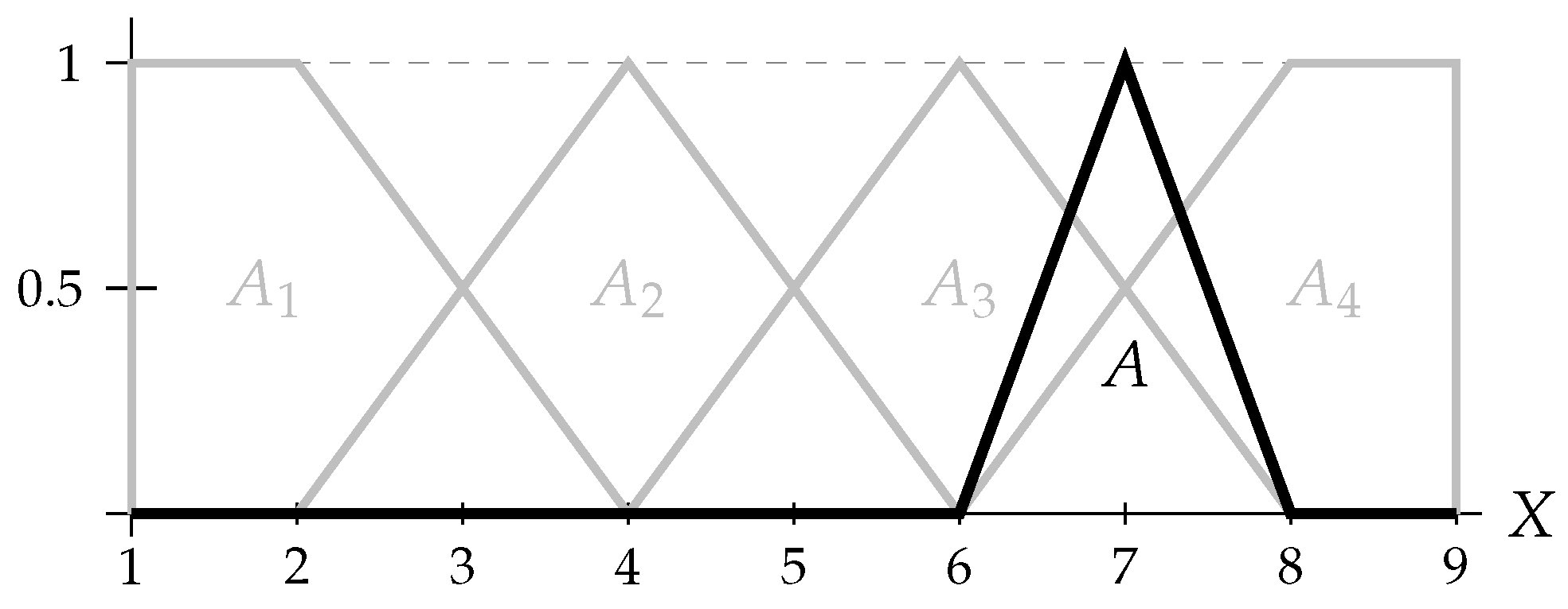
Let $(X,Y,{\mathcal{A}}_X,{\mathcal{B}}_Y)$ be the frame and Γ the $KB$ defined in Example 3, where a study on the heart rate (in bpm) (Y) in children between 1 and 9 years old (X) is conducted. In this example, the greatest model of Γ, ${\mathbf{M}}_{\Gamma }$, was plotted in Figure 6. Suppose that we want to study the possible heart rate of a child who is 30 months old, that is, two and a half years old. This case is translated on the frame $(X,Y,{\mathcal{A}}_X,{\mathcal{B}}_Y)$ as a crisp singleton $KB$-input $A\in \mathcal{F}\left(X\right)$, whose membership function is given below in Figure 7:

$$\begin{array}{c}\hfill A\left(x\right)=\left\{\begin{array}{cc}1& \mathit{if}x=2.5\hfill \\ 0& \mathit{otherwise}\hfill \end{array}\right.\end{array}$$

Figure 7. Membership function of $KB$-input A (bold) in Example 5 together with partition ${\mathcal{A}}_X$ (grey). The dashed line represents the discontinuity in the membership function of A.

The inference engine consists of the application of the GMP based on the f-index of inclusion for each of the elements in Γ. Since ${\mathcal{A}}_X$ has 4 elements and ${\mathcal{B}}_Y$ has 3 elements, we apply a total of $4·3=12$ GMP as described in Theorem 12:

$$\{⟨A_i\to B_j;f_{ij}⟩,A\}\vDash B_{ij},$$

where $B_{ij}\in \mathcal{F}\left(Y\right)$ is described in terms of Equation (3):

$$B_{ij}={\overline{\mathrm{Inc}}}_{\mathcal{G}}(A,A_i)\circ \overline{f}\left(B_j\left(y\right)\right).$$

Let us recall that $\overline{f}$ is the only mapping such that $(f_{ij},{\overline{f}}_{ij})$ forms an adjoint pair, as is ${\overline{\mathrm{Inc}}}_{\mathcal{G}}(A,A_i)$ with respect to the f-index of inclusion restricted to $\mathcal{G}$ of A in $A_i$. Therefore, in order to apply the GMP, it is necessary to compute each of the mappings ${\overline{f}}_{ij}$ and ${\overline{\mathrm{Inc}}}_{\mathcal{G}}(A,A_i)$. The following formula [30] allows us to compute the the adjoint pair associated with each $f_{ij}$ that appears in Γ by a straightforward manual calculation:

$${\overline{f}}_{ij}\left(\alpha \right)=\underset{\beta \in [0,1]}{sup}\{f_{ij}\left(\beta \right)\le \alpha \}$$

(5)

which results in the Table 5.

Table 5. Adjoint pairs associated with each one of the mappings on Table 3 in Example 3.

	$B_1$	$B_2$	$B_3$
$A_1$	$\mathbf{1}$	$\mathbf{1}$	${\overline{f}}_{0.5}$
$A_2$	$\mathbf{1}$	${\overline{f}}_{0.5}$	${\overline{g}}_{0.25}$
$A_3$	$\mathbf{1}$	${\overline{f}}_{0.75}$	$\mathbf{1}$
$A_4$	${\overline{f}}_{0.5}$	$\mathbf{1}$	$\mathbf{1}$

Where

$${\overline{g}}_n\left(\alpha \right)=\left\{\begin{array}{cc}n& \mathit{if}\alpha <n\\ 1& \mathit{if}\alpha \ge n,\end{array}\right.$$

$${\overline{f}}_n\left(\alpha \right)=\left\{\begin{array}{cc}\alpha & \mathit{if}\alpha <n\\ 1& \mathit{if}\alpha \ge n,\end{array}\right.$$

and $\mathbf{1}\left(\alpha \right)=1$ for all $\alpha \in [0,1]$.

Secondly, in order to apply the inference engine, the f-index of inclusion restricted to $\mathcal{G}$ of the $KB$-input A in each of the elements of the partition $A_i\in {\mathcal{A}}_X$ must be computed. The results obtained are as follows:

$${Inc}_{\mathcal{G}}(A,A_1)=f_{0.75},{Inc}_{\mathcal{G}}(A,A_2)=f_{0.25},{Inc}_{\mathcal{G}}(A,A_3)={Inc}_{\mathcal{G}}(A,A_4)=\mathbf{0}.$$

Nevertheless, the GMP defined in Theorem 12 employs the adjoint pair associated with each of these f-inclusions. By using the formula described in Equation (5), adapted for each ${Inc}_{\mathcal{G}}(A,A_i)$, we obtain each ${\overline{\mathrm{Inc}}}_{\mathcal{G}}(A,A_i)$, with $i=1,\dots ,4$:

$${\overline{\mathrm{Inc}}}_{\mathcal{G}}(A,A_1)={\overline{f}}_{0.75},{\overline{\mathrm{Inc}}}_{\mathcal{G}}(A,A_2)={\overline{f}}_{0.25},{\overline{\mathrm{Inc}}}_{\mathcal{G}}(A,A_3)={\overline{\mathrm{Inc}}}_{\mathcal{G}}(A,A_4)=\mathbf{1}.$$

Now, we can proceed to apply the GMP based on the f-index of inclusion restricted to $\mathcal{G}$. Let us first show an example of computation of this inference rule, considering the rule $⟨A_1\to B_3;f_{0.5}⟩$. The f-index of inclusion of the $KB$-input A into $A_1$ is $f_{0.75}$; then, according to Theorem 12, the result of applying GMP is

$$B_{13}\left(y\right)={\overline{f}}_{0.75}\circ {\overline{f}}_{0.5}\left(B_3\left(y\right)\right).$$

Note that this composition of mappings is applied to $B_3$; in other words, it does not depend on the $KB$-input A. Recall that the membership function of $B_3$ is:

$$B_3\left(y\right)=\left\{\begin{array}{cc}0& \mathit{if}y\in [70,100]\hfill \\ {\displaystyle \frac{y-100}{30}}& \mathit{if}y\in (100,130].\hfill \end{array}\right.$$

Let us compute the output step by step. The result of applying this fuzzy set to the mapping ${\overline{f}}_{0.5}$ is:

$${\overline{f}}_{0.5}\left(B_3\left(y\right)\right)=\left\{\begin{array}{cc}{B}_3\left(y\right)& \mathit{if}y\in [70,115)\hfill \\ 1& \mathit{if}y\in [115,130]\hfill \end{array}\right.=\left\{\begin{array}{cc}0& \mathit{if}y\in [70,100]\hfill \\ {\displaystyle \frac{y-100}{30}}& \mathit{if}y\in (100,115)\hfill \\ 1& \mathit{if}y\in [115,130].\hfill \end{array}\right.$$

Finally, the output of this GMP is:

$${\overline{f}}_{0.75}\circ {\overline{f}}_{0.5}\left(B_3\left(y\right)\right)=\left\{\begin{array}{cc}{\overline{f}}_{0.5}\left(B_3\left(y\right)\right)& \mathit{if}y\in [70,122.5)\hfill \\ 1& \mathit{if}y\in [122.5,130]\hfill \end{array}\right.=\left\{\begin{array}{cc}0& \mathit{if}y\in [70,100]\hfill \\ {\displaystyle \frac{y-100}{30}}& \mathit{if}y\in (100,115)\hfill \\ 1& \mathit{if}y\in [115,130].\hfill \end{array}\right.$$

In other words, applying the mapping ${\overline{f}}_{0.75}$ does not affect the final result.

In the vast majority of cases, we obtain the output $B_{ij}=Y$ due to the appearance of the top element $\mathbf{1}$ as one of the components of the function composition. All these cases are consequences of two possibilities: either the respective rule in Γ determines no restriction or the inclusion of A into $A_i$ is null. Recall that the final inference is the intersection of all the outputs $B_{ij}$; hence, all these cases are degenerate and do not produce any restriction. Accordingly, only those outputs where the mapping $\mathbf{1}$ is not involved in the application of the GMP are shown below:

$$\begin{array}{cc}\hfill & B_{13}\left(y\right)={\overline{f}}_{0.75}\circ {\overline{f}}_{0.5}\left(B_3\left(y\right)\right)=\left\{\begin{array}{cc}{B}_1\left(y\right)& \mathit{if}y\in [70,115)\hfill \\ 1& \mathit{if}y\in [115,130],\hfill \end{array}\right.\hfill \\ \hfill & B_{22}\left(y\right)={\overline{f}}_{0.25}\circ {\overline{f}}_{0.5}\left(B_2\left(y\right)\right)=\left\{\begin{array}{cc}{B}_2\left(y\right)& \mathit{if}y\in [70,77.5)\hfill \\ 1& \mathit{if}y\in [77.5,122.5]\hfill \\ B_2\left(y\right)& \mathit{if}y\in [122.5,130),\hfill \end{array}\right.\hfill \\ \hfill & B_{23}\left(y\right)={\overline{f}}_{0.25}\circ {\overline{g}}_{0.25}\left(B_3\left(y\right)\right)=1(i.e.,B_{23}=Y)\hfill \end{array}$$

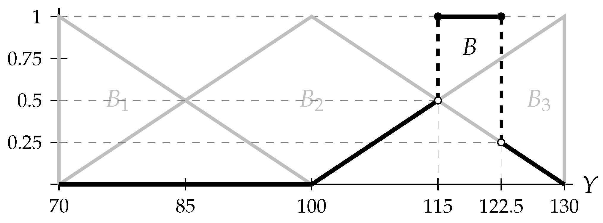
Once each of the inferences $B_{ij}$ is obtained, the $KB$-output is given by the fuzzy set B obtained by computing the intersection of each $B_{ij}$. Its membership function is given by:

$$B\left(y\right)=\bigcap _{\begin{array}{c}i\in \{1,2,3,4\}\\ j\in \{1,2,3\}\end{array}}{B}_{ij}\left(y\right)=\left\{\begin{array}{cc}0& \mathit{if}y\in [70,100]\hfill \\ {\displaystyle \frac{x-100}{30}}& \mathit{if}y\in (100,115)\hfill \\ 1& \mathit{if}y\in [115,122.5]\hfill \\ {\displaystyle \frac{130-x}{30}}& \mathit{if}y\in (122.5,130].\hfill \end{array}\right.$$

Figure 8 shows the membership function of this fuzzy set.

Figure 8. $KB$-output (bold line) obtained by applying the inference engine from $\Gamma$ and A in Example 5. The dashed line represents the discontinuity in the membership function of the $KB$-output.

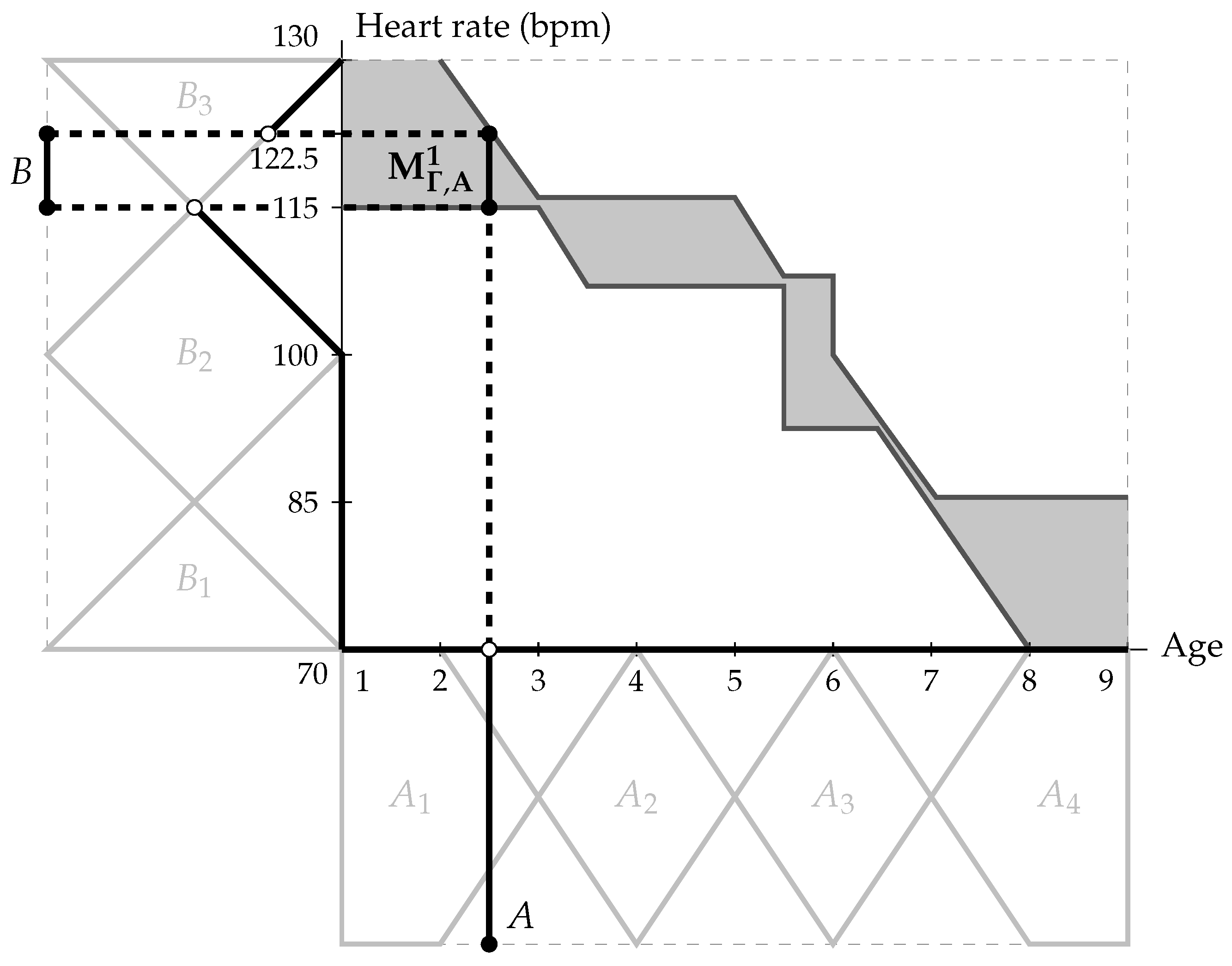
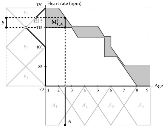
Finally, let us study the greatest model of $\Gamma \cup \left\{A\right\}$. Unlike the greatest model of Γ, ${\mathbf{M}}_{\Gamma ,\mathbf{A}}$ is a fuzzy set, and therefore, it may be difficult to represent its membership function on the plane $X\times Y$; instead, we can consider their α-cuts to study the relation between the $KB$-output and the greatest model. Since the $KB$-input A is a crisp singleton (i.e., A only takes values in $\{0,1\}$), let us consider the core (i.e., the 1-cut) of the $KB$-output B, which is represented in Figure 9. Its algebraic expression is:

$$core\left({\mathbf{M}}_{\Gamma ,\mathbf{A}}\right)=\{(x,y)\in X\times Y\mid x=2.5,y\in [115,122.5]\}.$$

(6)

Figure 9. $core\left({\mathbf{M}}_{\Gamma ,\mathbf{A}}\right)$ represented together with $KB$-input A and $KB$-output B from Example 5 (bold lines). The shaded region represents the greatest model of $\Gamma$.

Observe that for every element $(x,y)\in core\left({\mathbf{M}}_{\Gamma ,\mathbf{A}}\right)$, the X-component is contained in the core of A, and the Y-component is contained in the core of B, which is the interval $[115,122.5]$, that is,

$$core\left({\mathbf{M}}_{\Gamma ,\mathbf{A}}\right)=core\left(KB\text{-}\mathit{input}\right)\times core\left(KB\text{-}\mathit{output}\right).$$

Later on, we demonstrate that this phenomenon is not a coincidence. This result is used to justify the defuzzification procedure of our inference system, as can be seen in the following section.

Let us see now another example of application of the inference engine, this time involving a fuzzy set as $KB$-input with a continuous membership function.

Example 6.

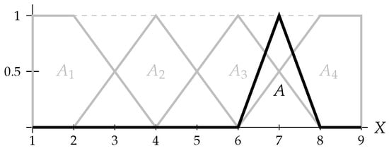
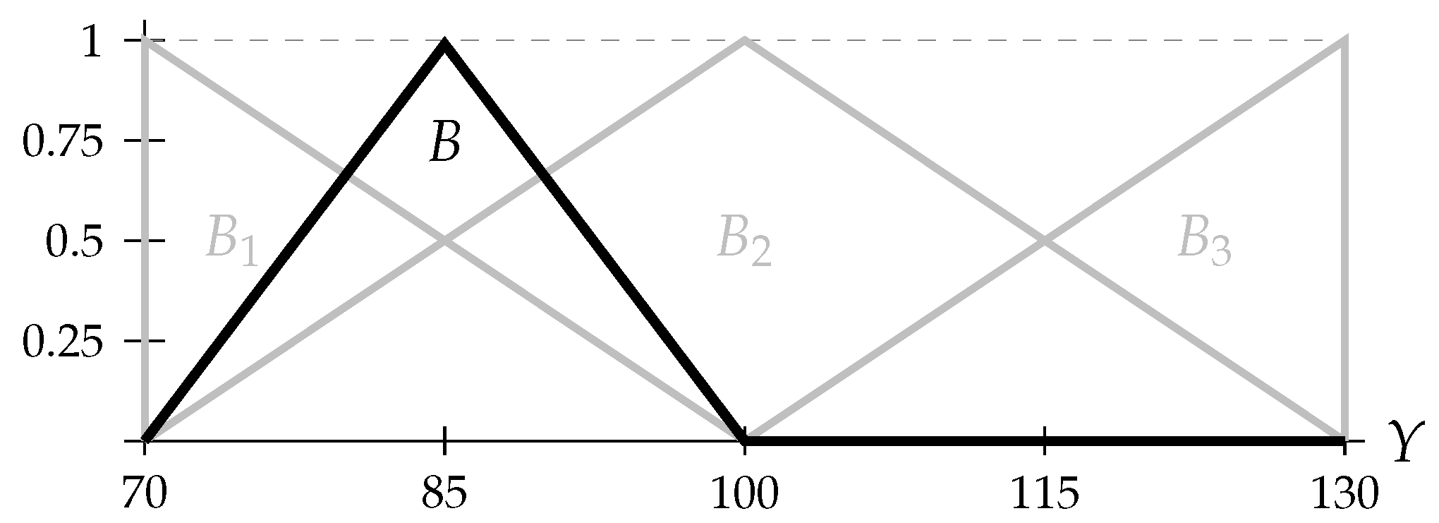
Consider the same frame $(X,Y,{\mathcal{A}}_X,{\mathcal{B}}_Y)$ and the same $KB$ Γ defined in Examples 3 and 5. Suppose now that we want to study the heart rate of a child who is “approximately seven years old”. This statement is represented by the $KB$-input $A\in \mathcal{F}\left(X\right)$ defined in Figure 10.

Figure 10. Membership function of $KB$-input A (bold) in Example 6 together with partition ${\mathcal{A}}_X$ (grey).

Just like in the previous example, 12 GMP based on the f-index of inclusion have to be carried out. Each one generates an output $B_{ij}$ given by the following expression:

$$B_{ij}={\overline{\mathrm{Inc}}}_{\mathcal{G}}(A,A_i)\circ \overline{f}\left(B_j\left(y\right)\right),$$

where $A_i\in {\mathcal{A}}_X$ and $B_j\in {\mathcal{B}}_Y$. Let us now compute each f-index of inclusion of the $KB$-input A in each element of the partition $A_i\in {\mathcal{A}}_X$:

$$Inc(A,A_1)=Inc(A,A_2)=\mathbf{0},\hspace{1em}\hspace{1em}\hspace{1em}\hspace{1em}Inc(A,A_3)=Inc(A,A_4)={\displaystyle \frac{id}{2}}.$$

$$\begin{array}{c}\hfill A\left(x\right)=\left\{\begin{array}{cc}0& \mathit{if}x\in [1,6]\hfill \\ x-6& \mathit{if}x\in (6,7]\hfill \\ 8-x& \mathit{if}x\in (7,8]\hfill \\ 0& \mathit{if}x\in (8,9].\hfill \end{array}\right.\end{array}$$

Let us now compute the mapping $\overline{{\displaystyle \frac{id}{2}}}$ such that $({\displaystyle \frac{id}{2}},\overline{{\displaystyle \frac{id}{2}}})$ forms an adjoint pair by using Equation (5):

$$\overline{{\displaystyle \frac{id}{2}}}\left(\alpha \right)=\left\{\begin{array}{cc}2x& \mathit{if}\alpha \in [0,0.5)\hfill \\ 1& \mathit{if}\alpha \in [0.5,1].\hfill \end{array}\right.$$

Only two outputs $B_{ij}$ different from Y are obtained, and they are given by those GMP obtained by applying rules $⟨A_3\to B_2;f_{0.75}⟩$ and $⟨A_4\to B_1;f_{0.5}⟩$:

$$\begin{array}{cc}\hfill & B_{32}=\overline{{\displaystyle \frac{id}{2}}}\circ {\overline{f}}_{0.75}\left(B_2\left(y\right)\right)=\left\{\begin{array}{cc}2·B_2\left(y\right)& \mathit{if}y\in [70,85)\hfill \\ 1& \mathit{if}y\in [85,115]\hfill \\ 2·B_2\left(y\right)& \mathit{if}y\in (115,130],\hfill \end{array}\right.\hfill \\ \hfill & B_{41}=\overline{{\displaystyle \frac{id}{2}}}\circ {\overline{f}}_{0.5}\left(B_1\left(y\right)\right)=\left\{\begin{array}{cc}1& \mathit{if}y\in [70,85]\hfill \\ 2·B_1\left(y\right)& \mathit{if}y\in (85,130].\hfill \end{array}\right.\hfill \end{array}$$

The final inference is obtained through the intersection of each output of the 12 GMP, which results in $B_{32}\cap B_{41}$. This $KB$-output is represented in Figure 11, and it is given by the following expression:

$$B\left(y\right)=\bigcap _{\begin{array}{c}i\in \{1,2,3,4\}\\ j\in \{1,2,3\}\end{array}}{B}_{ij}\left(y\right)=\left\{\begin{array}{cc}{\displaystyle \frac{x-70}{15}}& \mathit{if}y\in [70,85)\hfill \\ {\displaystyle \frac{100-x}{15}}& \mathit{if}y\in [85,100)\hfill \\ 0& \mathit{if}y\in [100,130].\hfill \end{array}\right.$$

Figure 11. $KB$-output (bold) obtained by applying the inference engine from $\Gamma$ and A in Example 6 together with partition ${\mathcal{B}}_Y$ (grey).

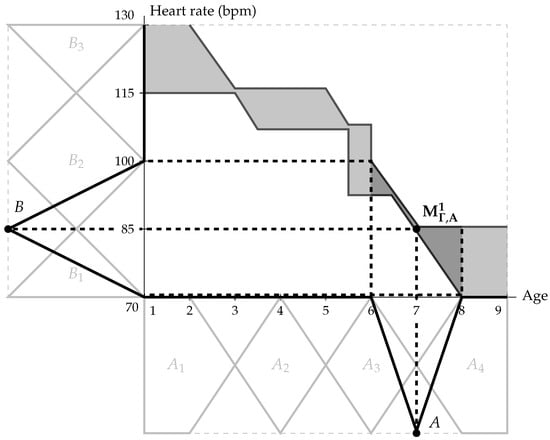
Finally, let us study the greatest model of $\Gamma \cup \left\{A\right\}$, as in the previous example. In Figure 12, we have represented the $KB$-input A, the $KB$-output B, and the core of the greatest model of $\Gamma \cup \left\{A\right\}$. In this case, we can also check that this set can be rewritten in terms of the cores of both A and B, namely, $core\left({\mathbf{M}}_{\Gamma ,\mathbf{A}}\right)=core\left(A\right)\times core\left(B\right)=\left\{(7,85)\right\}$. Moreover, there is an additional property satisfied by the greatest model ${\mathbf{M}}_{\Gamma ,\mathbf{A}}$, which is related to the support of ${\mathbf{M}}_{\Gamma ,\mathbf{A}}$ (represented in Figure 12 by the shaded region within ${\mathbf{M}}_{\Gamma }$), the support of A, and the support of B: $supp\left(A\right)$ is contained in the X-component of $supp\left(M\right)$, and $supp\left(B\right)$ is contained in its Y-component.

Figure 12. $core\left({\mathbf{M}}_{\Gamma ,\mathbf{A}}\right)$ and $supp\left({\mathbf{M}}_{\Gamma ,\mathbf{A}}\right)$ (dark gray) together with $KB$-input A and $KB$-output B (bold lines) from Example 6. The shaded region represents the greatest model of $\Gamma$ and auxiliary lines are represented in dashed.

Nevertheless, this last property is not always satisfied by the $KB$-output of a $KB$ Γ and a $KB$-input; e.g., the $KB$-output obtained in Example 5 has a greater support than the Y-component of $supp\left({\mathbf{M}}_{\Gamma ,\mathbf{A}}\right)$ (see Figure 9).

4.4. On Fuzzification and Defuzzification Procedures

Last but not least, we discuss the procedures of fuzzification and defuzzification. The reason is mainly because firstly, they depend strongly on the particular context of application of the inference system, and secondly, the scope of this paper is to show the correctness of the inference system. Nevertheless, here, we present some discussions and some issues to be considered in further approaches.

Obviously, the definition of rules in the knowledge database requires a pair of fuzzy partitions ${\mathcal{A}}_X$ and ${\mathcal{B}}_Y$ on the universes X and Y, respectively. That is a fuzzification procedure, but there is another that transforms the input of the system into a $KB$-input. In most approaches, the same fuzzy partitions used in the construction of the knowledge database are used to fuzzify the input of the system. However, in our approach, the $KB$-input may be any fuzzy set defined independently from the fuzzy partition ${\mathcal{A}}_X$ considered in X for the construction of the $KB$. That opens an endless number of possibilities for transforming the input of the fuzzy inference system into the $KB$-input. For instance, consider that for the sake of accuracy, we use two fuzzy partitions ${\mathcal{A}}_X$ and ${\mathcal{B}}_Y$ on the universes X and Y with hundreds of fuzzy sets each. On the other hand, in order to keep an interpretable input and output of the fuzzy inference system, we use linguistic labels in the form of fuzzy sets on X. These linguistic labels may have more or less elements, may be defined differently for each user, and may even have no relation with the partition ${\mathcal{A}}_X$ used in X for the $KB$. In all cases, given a linguistic label as a fuzzy set on X, we can reason with the $KB$.

Another possibility for a fuzzification is to iterate fuzzy inference systems, and then, the $KB$-output of one fuzzy inference system becomes the $KB$-input of the next one, so the fuzzification is then the result of a fuzzy inference system. Note that we can even not consider any fuzzification. That is, given a value or an interval of values in X (i.e., a crisp input), we can consider it as a set (or a singleton as a set as in Example 5) and then reason with it. As mentioned above, the fuzzy partitions considered in the construction of knowledge databases do not limit the fuzzification procedure for the $KB$-input; it is open to any possible fuzzification.

On the other hand, the defuzzification also depends on the scope of the application rather than the fuzzification. Therefore, it is hard to talk about it in this approach. Nevertheless, it is convenient to bear in mind the following characteristic of our fuzzy inference systems. The consideration of crisp models for the semantics of $KB$ allows us to focus on models as a defuzzification procedure. In this respect, we have two options, to either take into consideration all the possible values that are coherent with the modeling of a $KB$ and the $KB$-input (which results in choosing the greatest model as the (crisp) output of our system) or to focus on selecting a specific kind of model. This latter case is certainly more interesting, and the characteristics of these models depend on the scope of the application; for example, a regression model focuses on a functional model, whereas a classification model may focus on measure models with a certain $y\in Y$ in the second component.

It is worth finishing this section by focusing on the simplest case of fuzzification and defuzzification procedures: a singleton crisp input and the search for a set of possible values for the variable Y in the output. This is exactly the case illustrated in Example 5, were the crisp value $x=2.5$ is directly considered as a crisp-singleton fuzzy set as $KB$-input. The following result shows that in that case, the core of the $KB$-output determines the greatest model. Note that given $x_0\in X$, the singleton $\left\{x_0\right\}$ can be interpreted as the fuzzy set A such that $A\left(x_0\right)=1$ and $A\left(x\right)=0$ if $x\ne x_0$.

Corollary 5.

Let Γ be a $KB$ on a frame $(X,Y,{\mathcal{A}}_X,{\mathcal{B}}_Y)$, let $x_0\in X$, let M be the greatest model of $\Gamma \cap \left\{x_0\right\}$ and let B be the fuzzy set obtained in Equation (4) as the $KB$-output of $\Gamma \cap \left\{x_0\right\}$. Then, M is a crisp set (i.e., $M(x,y)\in \{0,1\}$) and

$$M(x_0,y)=1\mathit{if}\mathit{and}\mathit{only}\mathit{if}B\left(y\right)=1$$

Proof. 

Proving that M is crisp comes directly from Definitions 18 and 19, since all $\alpha$-models of $\left\{x_0\right\}$ coincide with the one-model of $\left\{x_0\right\}$.

Let us prove the “if and only if” part. By definition of a consequence and the correctness of Corollary 4, $M(x,y)=1$ implies $B\left(y\right)=1$. In other words, to prove the other implication, let us assume that $B\left(y\right)=1$. By definition of the inference engine in terms of intersections, we have that necessarily, for all rules $⟨A_i\to B_j;f_{ij}⟩\in \Gamma$,

$$B_{ij}\left(y\right)={\overline{\mathrm{Inc}}}_{\mathcal{G}}(\left\{x_0\right\},A_i)\circ {\overline{f}}_{ij}\left(B_j\left(y\right)\right)=1$$

Moreover, since $\left\{x_0\right\}$ is a singleton, it can be proved that

$${Inc}_{\mathcal{G}}(\left\{x_0\right\},A_i)\left(x\right)=\left\{\begin{array}{cc}{A}_i\left(x_0\right)\hfill & \mathrm{if}x\le A_i\left(x_0\right)\hfill \\ x\hfill & \mathrm{otherwise}.\hfill \end{array}\right.$$

Then, we have the following chain of inequalities:

$$\begin{array}{cc}\hfill & 1\le B_{ij}\left(y\right)={\overline{\mathrm{Inc}}}_{\mathcal{G}}(\left\{x_0\right\},A_i)\circ {\overline{f}}_{ij}\left(B_j\left(y\right)\right)\hfill \\ \hfill \iff & {Inc}_{\mathcal{G}}(\left\{x_0\right\},A_i)\left(1\right)\le {\overline{f}}_{ij}\left(B_j\left(y\right)\right)\hfill \\ \hfill \iff & A_i\left(x_0\right)\le {\overline{f}}_{ij}\left(B_j\left(y\right)\right)\hfill \\ \hfill \iff & f\left(A_i\left(x_0\right)\right)\le B_j\left(y\right).\hfill \end{array}$$

In other words, $(x_0,y)$ satisfies all the rules in $\Gamma$, and $\left\{(x_0,y)\right\}$ is a model of $\Gamma$. Moreover, since the $KB$-input is crisp, $\left\{(x_0,y)\right\}$ is a one-model of $\Gamma \cap \left\{x_0\right\}$. By maximality of M, necessarily, we have that $M(x_0,y)=1$, which is what we wanted to prove. □

In other words, in the case of working in the simplest setting of fuzzification (a crisp entry) and defuzzification (interval of plausible values in the greatest model), the values in the core of the $KB$-output directly determine the greatest model of the $KB$ and the $KB$-input. That fact is illustrated in the following example.

Example 7.

Let us reconsider Example 5, where the $KB$-input was the crisp singleton set $\left\{2.5\right\}$. The result of the fuzzy engine is

$$B\left(y\right)=\bigcap _{\begin{array}{c}i\in \{1,2,3,4\}\\ j\in \{1,2,3\}\end{array}}{B}_{ij}\left(y\right)=\left\{\begin{array}{cc}0& \mathit{if}y\in [70,100]\hfill \\ {\displaystyle \frac{x-100}{30}}& \mathit{if}y\in (100,115)\hfill \\ 1& \mathit{if}y\in [115,122.5]\hfill \\ {\displaystyle \frac{130-x}{30}}& \mathit{if}y\in (122.5,130].\hfill \end{array}\right.$$

whose core is the interval $[115,122.5]$. From Corollary 5, we can conclude that the greatest model of $\Gamma \cup \left\{2.5\right\}$ is

$$M=\{(x,y)\in {\mathbb{R}}^2\mid x=2.5\mathit{and}y\in [115,122.5]\}$$

The reader can check in Figure 9 that effectively, all pairs of values $(x,y)\in X\times Y$ in the greatest model of Γ with $x=2.5$ are exactly the interval $[115,122.5]$.

5. Comparison with Relational Fuzzy Inference Systems

Now that the FIS based on the notion of f-inclusion has been introduced, we can better describe the similarities and differences with the existing FISs in the literature. Let us recall that, as mentioned in the Introduction, there exist two families of FISs, namely, the so-called relational fuzzy inference systems and those based on aggregating crisp values (or entities). Our approach is mainly related to the former ones, because they consider relations to link universes (the one of the antecedent and the one of the consequent), because the result of the inference is a fuzzy set, which needs a defuzzification procedure, and because, as we show below, the f-index of inclusion can be related to a pair formed by a fuzzy conjunction and a fuzzy implication.

In the family of relational FISs, we have two main models, the Mamdani and the implicative models [3], which have the following general form: given two sets X and Y, a set of rules

$$\mathrm{If}x\mathrm{is}{A}_i\mathrm{THEN}y\mathrm{is}{B}_{i}i=1,\dots n$$

with $A_i\in \mathcal{F}\left(X\right)$ and $B_i\in \mathcal{F}\left(Y\right)$, an adjoint pair $(\ast ,\to )$ (although in many papers, the choice of the fuzzy conjunction and implication looks general, the truth is that without the adjointness property, results may be unexpected [3,31]), and a fuzzy set $A^{\prime }\in \mathcal{F}\left(X\right)$ as input, the inference $B^{\prime }\in \mathcal{F}\left(Y\right)$ is performed in the implicative model by

$$B^{\prime }\left(y\right)=(A^{\prime }\circ R)\left(y\right)=\underset{x\in X}{\bigvee }{A}^{\prime }\left(x\right)\ast R(x,y)$$

where the relation R is defined as

$$R(x,y)=\underset{i}{\overset{n}{\bigwedge }}{A}_i\left(x\right)\to B_i\left(y\right)$$

and in the Mamdani model by

$$B^{\prime }\left(y\right)=(A^{\prime }⊳R)\left(y\right)=\underset{x\in X}{\bigwedge }{A}^{\prime }\left(x\right)\to R(x,y)$$

where the relation R is defined as

$$R(x,y)=\underset{i}{\overset{n}{\bigvee }}{A}_i\left(x\right)\ast B_i\left(y\right).$$

These two formulae turn into the two following general forms:

$$\underset{x\in X}{\bigvee }\left(A^{\prime }\left(x\right)\ast \underset{i}{\overset{n}{\bigwedge }}{A}_i\left(x\right)\to B_i\left(y\right)\right)\mathrm{and}\underset{x\in X}{\bigwedge }\left(A^{\prime }\left(x\right)\to \underset{i}{\overset{n}{\bigvee }}{A}_i\left(x\right)\ast B_i\left(y\right)\right).$$

(7)

Here, we can see a clear difference. Whereas in standard relational FISs, the relations are the core of the inference engine, in the proposed FIS based on f-inclusion, the relations belong to the semantics, providing to the approach a formal logic support. Here, it is convenient to recall the following result from [15]: given $f\in \mathcal{G}$, there exists an adjoint pair $(\ast ,\to )$ with * a commutative fuzzy conjunction and $\alpha \in [0,1]$ such that

$$f\left(x\right)=x\ast \alpha .$$

Moreover, if f is the f-index of inclusion of two fuzzy sets A and B on the universe $\mathcal{U}$, then

$$\alpha =\underset{u\in \mathcal{U}}{\bigwedge }A\left(u\right)\to B\left(u\right).$$

Let us recall that in the FIS based on f-inclusion, rules are weighted by f-inclusions. If those weights are interpreted as the f-index of inclusion between antecedent and consequent, then we have that for each rule

$$⟨A_i\to B_j:f_{ij}⟩$$

there exists an adjoint pair $({\ast }_{ij},{\to }_{ij})$ mapping $f_{ij}$ with the form

$$f_{ij}\left(z\right)=z{\ast }_{ij}\left(\underset{(x,y)\in X\times Y}{\bigwedge }{A}_i\left(x\right){\to }_{ij}{B}_j\left(y\right)\right)$$

and its respective right adjoint with the form

$${\overline{f}}_{ij}\left(z\right)=\left(\underset{(x,y)\in X\times Y}{\bigwedge }{A}_i\left(x\right){\to }_{ij}{B}_j\left(y\right)\right){\to }_{ij}z.$$

Consequently, and keeping the previous notation, the full inference for an input $A^{\prime }\in \mathcal{F}\left(X\right)$ given in Equation (4) is given by the following formula:

$$B^{\prime }\left(z\right)=\underset{\begin{array}{c}{A}_i\in {\mathcal{A}}_X\\ B_j\in {\mathcal{B}}_Y\end{array}}{inf}\left[\left(\underset{x\in X}{inf}{A}^{\prime }\left(x\right){\to }_{i}A\left(x\right)\right){\to }_i\left(\left(\underset{(x,y)\in X\times Y}{inf}{A}_i\left(x\right){\to }_{ij}{B}_j\left(z\right)\right){\to }_{ij}{B}_j\left(y\right)\right)\right]$$

(8)

Here, we can clearly see the difference between the inference performance of our approach (Equation (8)) with the standard relational FIS (Equation (7)).

At this point, and due to the intricate pattern of Equation (8), it is worth focusing on the simplicity of our approach. The formulation of our inference engine, shown in Equation (4), is

$$B^{\prime }\left(y\right)=\underset{\begin{array}{c}{A}_i\in {\mathcal{A}}_X,\\ B_j\in {\mathcal{B}}_Y\end{array}}{inf}{\overline{\mathrm{Inc}}}_{\mathcal{G}}(A^{\prime },A_i)\circ {\overline{f}}_{ij}\left(B_j\left(y\right)\right),$$

Therefore, our inference is just the intersection of the inference performed by each rule in the $KB$. In turn, the inference performed by each rule $A_i\to B_j$ is just the composition of two mappings:

• ${\overline{f}}_{ij}$ that represents the inclusion of the antecedent in the consequent;
• ${\overline{\mathrm{Inc}}}_{\mathcal{G}}(A^{\prime },A_i)$ that represents the inclusion of the input in the antecedent of the respective rule.

Note that we do not need to consider any adjoint pair of fuzzy conjunctions and implications to perform the inference, we only take mappings in $\mathcal{G}$, i.e., Equation (8) is purely theoretical.

6. Conclusions and Future Works

In this article, we showed how to define a fuzzy inference system (FIS) in terms of the notion of f-inclusion. The main difference between this FIS and the ones from the literature is that it is based on a formal logic background. Indeed, we related the models of our knowledge databases with models of a certain Fuzzy Description Logic (FDL) ${\mathcal{LU}}_{FH}$, which consists of the standard FDL $\mathcal{LU}$ enriched with modifiers (or fuzzy hedges). This connection allowed us to apply inferences from ${\mathcal{LU}}_{FH}$ in our FIS based on f-inclusion, allowing us to use a Generalized Modus Ponens (GMP) in our inference engine. Another advantage of our FIS is that it allowed us to consider any fuzzy set as input of the inference engine. That allowed us to consider fuzzy partitions for the construction of the knowledge database independently on the fuzzification used to transform the input of the FIS into the inference engine. For example, we can consider any set of linguistic labels in our FIS independently from the fuzzy partitions used to define the knowledge database.

From a theoretical point of view, we highlight the following achievements. First, we defined the notion of the consequence of a FIS, which allowed us to prove the correctness of the proposed inference engine. Second, we proved convenient properties of the consequences of a knowledge database and an input concerning monotony and a lattice algebraic structure. Finally, we reduced the search of consequences to the computation of the greatest model.

This approach opens an interesting number of future research lines. First, in this article, we focused on the theoretical correctness of the FIS. Therefore, it is necessary to define more application-oriented procedures aimed at defining knowledge databases from data. Because of the properties of the f-index of inclusion and the definition of the $KB$, we believe that we can define easy machine learning methods for rules in our FIS based on f-inclusion. Second, additional theoretical properties of the set of consequences in our FIS are necessary to provide stronger support for our approach. Along this line, to obtain a completeness inference engine would be ideal. Finally, applications of this FIS to real applied domains are welcome and of interest to the authors. Since the semantics of the FIS is inspired by Fuzzy Description Logic, we expect to have applications of this FIS based on f-inclusion in the development of expert systems, although we do not discard other applications, such as in classification or control systems.

References

- Mamdani, E.; Assilian, S. An experiment in linguistic synthesis with a fuzzy logic controller. Int. J. Man-Mach. Stud. 1975, 7, 1–13. [Google Scholar] [CrossRef]
- Eghbal Ahmadi, M.H.; Royaee, S.J.; Tayyebi, S.; Bozorgmehry Boozarjomehry, R. A new insight into implementing Mamdani fuzzy inference system for dynamic process modeling: Application on flash separator fuzzy dynamic modeling. Eng. Appl. Artif. Intell. 2020, 90, 103485. [Google Scholar] [CrossRef]
- Štěpnička, M.; Jayaram, B.; Su, Y. A short note on fuzzy relational inference systems. Fuzzy Sets Syst. 2018, 338, 90–96. [Google Scholar] [CrossRef]
- Daňková, M. On approximate reasoning with graded rules. Fuzzy Sets Syst. 2007, 158, 652–673. [Google Scholar] [CrossRef][Green Version]
- Sugeno, M. Industrial Applications of Fuzzy Control; Elsevier Science Ltd.: Amsterdam, The Netherlands, 1985. [Google Scholar]
- Gupta, P.K.; Muhuri, P.K. Extended Tsukamoto’s inference method for solving multi-objective linguistic optimization problems. Fuzzy Sets Syst. 2019, 377, 102–124. [Google Scholar] [CrossRef]
- Perfilieva, I.; Novák, V.; Dvořák, A. Fuzzy transform in the analysis of data. Int. J. Approx. Reason. 2008, 48, 36–46. [Google Scholar] [CrossRef]
- Madrid, N. Significance measures for rules in probabilistic-fuzzy inference systems based on fuzzy transforms. Fuzzy Sets Syst. 2023, 467, 108575. [Google Scholar] [CrossRef]
- Benzaouia, A. Switching Takagi-Sugeno Systems. In Saturated Switching Systems; Springer London: London, UK, 2012; pp. 247–274. [Google Scholar] [CrossRef]
- Koohathongsumrit, N.; Meethom, W. An integrated approach of fuzzy risk assessment model and data envelopment analysis for route selection in multimodal transportation networks. Expert Syst. Appl. 2021, 171, 114342. [Google Scholar] [CrossRef]
- Veeramani, C.; Venugopal, R.; Muruganandan, S. An Exploration of the Fuzzy Inference System for the Daily Trading Decision and Its Performance Analysis Based on Fuzzy MCDM Methods. Comput. Econ. 2023, 62, 1313–1340. [Google Scholar] [CrossRef]
- Cao, J.; Zhou, T.; Zhi, S.; Lam, S.; Ren, G.; Zhang, Y.; Wang, Y.; Dong, Y.; Cai, J. Fuzzy inference system with interpretable fuzzy rules: Advancing explainable artificial intelligence for disease diagnosis—A comprehensive review. Inf. Sci. 2024, 662, 120212. [Google Scholar] [CrossRef]
- Madrid, N.; Ojeda-Aciego, M.; Perfiljeva, I. ƒ-inclusion indexes between fuzzy sets. In Proceedings of the Conference of the International Fuzzy Systems Association and the European Society for Fuzzy Logic and Technology, Riga, Latvia, 21–25 July 2025; pp. 1528–1533. [Google Scholar] [CrossRef]
- Díaz-Montarroso, C.; Madrid, N.; Ramírez-Poussa, E. Towards a Generalized Modus Ponens Based on the f-Index of Inclusion. In Proceedings of the Conceptual Knowledge Structures: First International Joint Conference, CONCEPTS 2024, Cádiz, Spain, 9–13 September 2024; pp. 36–48. [Google Scholar] [CrossRef]
- Madrid, N.; Ojeda-Aciego, M. The f-index of inclusion as optimal adjoint pair for fuzzy modus ponens. Fuzzy Sets Syst. 2023, 466, 108474. [Google Scholar] [CrossRef]
- Madrid, N.; Ojeda-Aciego, M. Functional degrees of inclusion and similarity between L-fuzzy sets. Fuzzy Sets Syst. 2020, 390, 1–22. [Google Scholar] [CrossRef]
- Straccia, U. A fuzzy description logic. In Proceedings of the AAAI/IAAI, 1998, Madison, WI, USA, 26–30 July 1998; pp. 594–599. [Google Scholar]
- Godo, L.; Hájek, P. Fuzzy Inference as Deduction. J. Appl. Non-Class. Logics 1999, 9, 37–60. [Google Scholar] [CrossRef][Green Version]
- Hájek, P.; Paris, J.; Shepherdson, J. Rational Pavelka Predicate Logic is a Conservative Extension of Łukasiewicz Predicate Logic. J. Symb. Log. 2000, 65, 669–682. [Google Scholar] [CrossRef]
- Flaminio, T.; Marchioni, E. T-norm-based logics with an independent involutive negation. Fuzzy Sets Syst. 2006, 157, 3125–3144. [Google Scholar] [CrossRef]
- Hölldobler, S.; Khang, T.D.; Störr, H.P. A Fuzzy Description Logic with Hedges as Concept Modifiers. In Proceedings of the InTech/VJFuzzy’2002; Phuong, N.H., Nguyen, H.T., Ho, N.C., Santiprabhob, P., Eds.; Science and Technics Publishing House: Hanoi, Vietnam, 2002; pp. 25–34. [Google Scholar]
- Madrid, N.; Ramírez-Poussa, E. Analysis of the f-index of inclusion restricted to a set of indexes. In Proceedings of the 20th International Conference on Information Processing and Management of Uncertainty in Knowledge-Based Systems (IPMU2024), Lisbon, Portugal, 22–26 July 2024. [Google Scholar]
- Madrid, N.; Ojeda-Aciego, M. Composition as a fuzzy conjunction between indexes of inclusion. Fuzzy Sets Syst. submitted.
- Sinha, D.; Dougherty, E. Fuzzification of Set Inclusion: Theory and Applications. Fuzzy Sets Syst. 1993, 55, 15–42. [Google Scholar] [CrossRef]
- Kitainik, L.M. Fuzzy Inclusions and Fuzzy Dichotomous Decision Procedures. In Optimization Models Using Fuzzy Sets and Possibility Theory; Kacprzyk, J., Orlovski, S.A., Eds.; Springer: Dordrecht, The Netherlands, 1987; pp. 154–170. [Google Scholar] [CrossRef]
- Birkhoff, G. Lattice Theory; Colloquium Publications, American Mathematical Society: Providence, RI, USA, 1940; Volume 25. [Google Scholar]
- Esteva, F.; Godo, L.; Noguera, C. Fuzzy logics with truth hedges revisited. In Proceedings of the 7th Conference of the European Society for Fuzzy Logic and Technology (EUSFLAT-11), Aix-Les-Bains, France, 18–22 July 2011; pp. 146–152. [Google Scholar] [CrossRef]
- Baldwin, J. A new approach to approximate reasoning using a fuzzy logic. Fuzzy Sets Syst. 1979, 2, 309–325. [Google Scholar] [CrossRef]
- Dubois, D.; Prade, H. What are fuzzy rules and how to use them. Fuzzy Sets Syst. 1996, 84, 169–185. [Google Scholar] [CrossRef]
- Ganter, B.; Wille, R. Formal Concept Analysis: Mathematical Foundations; Springer Science & Business Media: Berlin/Heidelberg, Germany, 1999. [Google Scholar]
- Novák, V.; Perfilieva, I.; Močkoř, J. Mathematical Principles of Fuzzy Logic; Springer: Boston, MA, USA, 1999. [Google Scholar] [CrossRef]
Disclaimer/Publisher’s Note: The statements, opinions and data contained in all publications are solely those of the individual author(s) and contributor(s) and not of MDPI and/or the editor(s). MDPI and/or the editor(s) disclaim responsibility for any injury to people or property resulting from any ideas, methods, instructions or products referred to in the content. |
© 2025 by the authors. Licensee MDPI, Basel, Switzerland. This article is an open access article distributed under the terms and conditions of the Creative Commons Attribution (CC BY) license (https://creativecommons.org/licenses/by/4.0/).