Stress Estimation in Viscous Flows Using an Iterative Tikhonov Regularized Stokes Inverse Model

Abstract

In this paper, we propose and develop a stationary Stokes Inverse Model (SIM) to estimate the stress distributions that are difficult to measure directly in flows. We estimate the driving stresses from the velocities by solving the inverse problem governed by Stokes equations under iterative Tikhonov (IT) regularization. We investigate the heuristic L-curve criterion to determine the proper regularization parameter. The solution existence and uniqueness for the Stokes inverse problem have been analyzed. We also conducted convergence analysis and error estimation for perturbed data, providing a fast and stable convergence. The finite element method is applied to the numerical approach. Following the theoretical investigation and formulation, we validate the model and demonstrate that the velocity data closely match the velocity fields that were reconstructed using the computed stress distributions. In particular, the proposed SIM can be used to reliably derive the stress distributions for the flows governed by the Stokes equations with small Reynolds number. Additionally, the model is robust to a certain number of perturbations, which enables the precise and effective estimation of the stress distributions. The proposed stationary SIM may be widely applicable in the estimation of stresses from experimental velocity fields in engineering and biological applications.

1. Introduction

For the fluid dynamic analysis of engineering and biological applications, the driving stresses are difficult to measure directly while the movements (e.g., velocity fields and displacements) are relatively easy to record. This discrepancy has driven significant advances in mathematical modeling techniques that estimate driving forces from observed kinematics. Current key methodologies for stress estimation are physics-based inverse solvers, such as the adjoint optimization or regularization strategies [1,2], and machine learning (ML)-driven approaches, such as Physics-Informed Neural Networks (PINNs) [3]. The inverse solvers, with the idea that determine the cause from the outcome, enable us to estimate the stresses (the cause) from the velocity data (the outcome) [4]. A key character of inverse problem is ill-posedness, which means the solution is not continuously dependent on the measured data, such that a small perturbation may induce a large deviation in the result [5]. The main approaches for solving inverse problems at present include regularization stabilizing solutions, variational methods balancing data fidelity and constraints, and Bayesian inference for probabilistic uncertainty quantification. ML speeds up processes like MRI reconstruction, whereas iterative techniques, such as Newton-type and gradient descent, deal with nonlinearity. Time-series data are integrated through data assimilation. New hybrid approaches by fusing physics and machine learning prioritize precision, effectiveness, and interpret ability in domains such as geophysics and medical imaging [1,2,3,5,6]. Among them, regularization is a well-developed strategy to overcome the ill-posedness of inverse problems, which consists of a regularization operator and a parameter choice rule [7]. The general idea of regularization is replacing the ill-posed problem to an approximating well-posed problem using a regularization operator. Additionally, for perturbed data, the approximate solutions converge to the desired solution as the noise level diminishes to zero. Regularization strategies for estimating stresses have been deployed and developed in a variety of practical applications. In engineering, hydrodynamic loads, like wave forces, for fatigue assessment are estimated under regularization using vibration data from bridges or offshore platforms [8]. In biology, Lauga, E. has been implicitly using Tikhonov regularization to elucidate the mechanism of microbial motility in a viscous dominant environment, which is governed by Stokes equations with small Reynolds number [9]. Tikhonov regularization, a well-known strategy, is stable and efficient [10]. However, the rate of convergence with respect to the noise level $\delta$ in the data cannot exceed a certain saturation level of $O({\delta }^{{\displaystyle \frac{2}{3}}})$ [11,12,13,14], while the iterative Tikhonov regularization may improve the convergence rate and has relatively high accuracy of approximation [15,16]. For solving the inverse problem governed by Stokes equations and stress estimation, studies on iterative Tikhonov (IT) regularization are not extensive. So we build an integrated Stokes Inverse Model (SIM) to solve it and estimate the stresses numerically through the IT regularization. The regularization parameter is a key component, which has a significant impact on accuracy and stability. Too large or too small a regularization parameter will lead to inaccuracy of the solution or computation instability [5]. Therefore, we have also discussed and compared the selecting methods of the optimal regularization parameters in SIM.

The Stokes Inverse Model (SIM) introduced in this paper is to solve the inverse problem governed by the incompressible Stokes fluid Equation (1) numerically to estimate the numerical stresses $\mathbf{f}$,

$$\left\{\begin{array}{cc}-\mu △\mathbf{u}+▽p=\mathbf{f},\hfill & \mathrm{in}\Omega ,\hfill \\ ▽·\mathbf{u}=0,\hfill & \mathrm{in}\Omega ,\hfill \\ \mathbf{u}=0,\hfill & \mathrm{on}\Gamma ,\hfill \end{array}\right.$$

(1)

where $\Omega \subset R^2$ is a bounded domain with boundary $\Gamma$. $\rho$ is the fluid density, $\mu$ is the dynamic viscosity of the fluid, $\mathbf{u}\left(\mathbf{x}\right)$ is the flow velocity at location $(x,y)$, p is the fluid pressure, and $\mathbf{f}$ is the stress that drives the flow movement. $▽·\mathbf{u}=0$ means the fluid is incompressible. We restrict our analysis to the homogeneous Dirichlet boundary condition that $\mathbf{u}{\mid }_{\Gamma }=0$.

The rest of this paper is laid out as follows: In Section 2, we describe the formulation procedure of the SIM. In Section 3, we present the Stokes inverse problem for the existence and uniqueness of the solution and provide the convergence rate of the IT regularization for solving it. In Section 4, we present the variational formulation and build the finite element scheme to compute the model numerically. In Section 5, we perform the model validation to confirm the model’s applicability. Finally, we summarize and discuss the work of this paper in Section 6.

2. Stokes Inverse Model (SIM) Formulation

In numerical fluid dynamics, non-dimensionalization is a critical step that highlights the prevailing physical mechanisms and prevents conflicts with the fluid unit system. So before formulating the model, we conducted the non-dimensionalization. We first introduce characteristic variables $L,U,P,F,and\left[\alpha \right]$, as defined in Table 1.

Table 1. Characteristic variables along with their primary units.

Characteristic Variables	Description	Primary Units
L	Characteristic length	$\mathrm{m}$
U	Characteristic velocity	$\mathrm{m} {\mathrm{s}}^{-1}$
$F={\displaystyle \frac{\rho U^2}{L}}$	Characteristic force	$\mathrm{k}\mathrm{g} {\mathrm{m}}^{-2}{\mathrm{s}}^{-2}$
$P={\displaystyle \frac{\mu U}{L}}$	Characteristic pressure	$\mathrm{k}\mathrm{g} {\mathrm{m}}^{-1}{\mathrm{s}}^{-2}$
$\left[\alpha \right]={\displaystyle \frac{L^2}{{\rho }^2{U}^2}}$	Characteristic regularization parameter	${\mathrm{m}}^6{\mathrm{s}}^2/\mathrm{k}{\mathrm{g}}^2$

Then, we compute the dimensionless variables from Equation (2).

$${\Gamma }^{*}={\displaystyle \frac{\Gamma }{L}},{\mathbf{u}}^{*}={\displaystyle \frac{\mathbf{u}}{U}},{\mathbf{f}}^{*}={\displaystyle \frac{\mathbf{f}}{F}},p^{*}={\displaystyle \frac{p}{P}},{\alpha }^{*}={\displaystyle \frac{\alpha }{\left[\alpha \right]}},{▽}^{*}=L▽$$

(2)

Substituting dimensionless variables into the Stokes equations and building the dimensionless Stokes iterative Tikhonov functional (3, 4), the driving stress distributions for given velocities were determined when the numerical velocity fields ${\mathbf{u}}^{*}$ match the given data ${\overline{\mathbf{u}}}^{*}$:

For every $n,n=1,\cdots ,N$,

$$min{J}_{{\alpha }^{*}}^{*}\left({\mathbf{f}}_n^{*}\right)={\displaystyle \frac{1}{2}}{\int }_{{\Omega }^{*}}|{\mathbf{u}}_n^{*}-{\overline{\mathbf{u}}}^{*}{|}^2\mathrm{d}{\mathbf{x}}^{*}+{\displaystyle \frac{{\alpha }^{*}}{2}}{\int }_{{\Omega }^{*}}{|{\mathbf{f}}_n^{*}-{\mathbf{f}}_{n-1}^{*}|}^2\mathrm{d}{\mathbf{x}}^{*}$$

(3)

subject to

$$\left\{\begin{array}{cc}-{\displaystyle \frac{1}{Re}}{△}^{*}{\mathbf{u}}_n^{*}+{\displaystyle \frac{1}{Re}}{▽}^{*}{p}_n^{*}={\mathbf{f}}_{n-1}^{*}+({\mathbf{f}}_n^{*}-{\mathbf{f}}_{n-1}^{*}),\hfill & \mathrm{in}{\Omega }^{*},\hfill \\ {▽}^{*}·{\mathbf{u}}_n^{*}=0,\hfill & \mathrm{in}{\Omega }^{*},\hfill \\ {\mathbf{u}}_n^{*}=0,\hfill & \mathrm{on}{\Gamma }^{*},\hfill \end{array}\right.$$

(4)

where $Re={\displaystyle \frac{\rho UL}{\mu }}$ is the Reynolds number, which is an important dimensionless parameter for studying the flow pattern and aiding in fluid behavior prediction [17,18,19]. ${\alpha }^{*}$ is the dimensionless regularization parameter.

To solve the Stokes inverse problem, we apply the Lagrange multiplier method, which is a powerful tool in optimization, particularly for problems with equality constraints. Introducing the Lagrange multipliers ${\mathbf{v}}_n$, $q_n$ to the domain ${\Omega }^{*}$, the Stokes iterative Tikhnov Lagrange functional is set up as Equation (5): For every $n,n=1,\cdots ,N$,

$$\begin{array}{ccc}\hfill & & L_n({\mathbf{u}}_n^{*},p_n^{*},{\mathbf{v}}_n^{*},q_n^{*},{\mathbf{f}}_n^{*})={\displaystyle \frac{1}{2}}{\int }_{{\Omega }^{*}}|{\mathbf{u}}_n^{*}-{\overline{\mathbf{u}}}^{*}{|}^2\mathrm{d}{\mathbf{x}}^{*}+{\displaystyle \frac{{\alpha }^{*}}{2}}{\int }_{{\Omega }^{*}}{|{\mathbf{f}}_n^{*}-{\mathbf{f}}_{n-1}^{*}|}^2\mathrm{d}{\mathbf{x}}^{*}\hfill \\ & & -{\int }_{{\Omega }^{*}}{\mathbf{v}}_n^{*}·(-{\displaystyle \frac{1}{Re}}{△}^{*}{\mathbf{u}}_n^{*}+{\displaystyle \frac{1}{Re}}{▽}^{*}{p}_n^{*}-{\mathbf{f}}_{n-1}^{*}-({\mathbf{f}}_n^{*}-{\mathbf{f}}_{n-1}^{*}))\mathrm{d}{\mathbf{x}}^{*}\hfill \\ & & -{\int }_{{\Omega }^{*}}{q}_n^{*}\left({▽}^{*}·{\mathbf{u}}_n^{*}\right)\mathrm{d}{\mathbf{x}}^{*}.\hfill \end{array}$$

(5)

In order to find the minimum solution of (3, 4), we derive the G $\widehat{a}$ teaux derivatives of $L_n({\mathbf{u}}_n^{*},p_n^{*},{\mathbf{v}}_n^{*},q_n^{*},{\mathbf{f}}_n^{*})$ with respect to ${\mathbf{u}}_n^{*},p_n^{*},{\mathbf{v}}_n^{*},q_n^{*},{\mathbf{f}}_n^{*}$ and make the derivatives to be 0. Then, the dimensionless Stokes iterative Tikhonov system with the boundary conditions (6) is formulated as follows:

For every $n,n=1,\cdots ,N$,

$$\{\begin{array}{ccc}-\frac{1}{\mathit{Re}}{∆}^{*}{\mathbf{u}}_n^{*}+\frac{1}{\mathit{Re}}{\nabla }^{*}{p}_n^{*}={\mathrm{f}}_{n-1}^{*}-\frac{{\mathbf{v}}_n^{*}}{{\alpha }^{*}},\hfill & \mathrm{in}{\Omega }^{*},& \hfill \mathrm{(6a)}\\ -{\nabla }^{*}·{\mathbf{u}}_n^{*}=0,\hfill & \mathrm{in}{\Omega }^{*},& \mathrm{(6b)}\\ {\mathbf{u}}_n^{*}=0,\hfill & \mathrm{on}{\Gamma }^{*},& \mathrm{(6c)}\\ -\frac{1}{\mathit{Re}}{∆}^{*}{\mathbf{v}}_n^{*}-{\nabla }^{*}{q}_n^{*}={\mathbf{u}}_n^{*}-{\overline{\mathbf{u}}}^{*},\hfill & \mathrm{in}{\Omega }^{*},& \mathrm{(6d)}\\ \frac{1}{\mathit{Re}}{\nabla }^{*}·{\mathbf{v}}_n^{*}=0,\hfill & \mathrm{in}{\Omega }^{*},& \mathrm{(6e)}\hfill \\ {\mathbf{v}}_n^{*}=0,\hfill & \mathrm{on}{\Gamma }^{*}.& \mathrm{(6f)}\end{array}$$

The optimal solution $({\mathbf{u}}_n^{*},p_n^{*},{\mathbf{v}}_n^{*},q_n^{*},{\mathbf{f}}_n^{*})$ will be computed by solving the Stokes iterative Tikhonov system. After N iterations, the inverse solution of the dimensionless numerical stress ${\mathbf{f}}_N^{*}$ is derived as Equation (7):

$${\mathbf{f}}_N^{*}={\mathbf{f}}_0^{*}-\sum _{n=1}^N{\displaystyle \frac{{\mathbf{v}}_n^{*}}{{\alpha }^{*}}}.$$

(7)

3. Existence, Uniqueness and Error Estimation

To confirm the accuracy of the SIM, we discuss the existence and uniqueness of the solution. Additionally, we do the convergence analysis and estimate the error for the SIM under the IT regularization.

3.1. Existence and Uniqueness of the Solution for the Stokes Inverse Problem

We first investigate the SIM for the existence and uniqueness of the solution. For the Stokes iterative Tikhonov functional $J_{\alpha }\left({\mathbf{f}}_n^{*}\right)$ (3, 4), let

$$\begin{array}{c}\hfill V:=\{\mathbf{u}\in {\left(H_0^1(\Omega )\right)}^2;▽·\mathbf{u}=0\}\subset {\left(H_0^1(\Omega )\right)}^2,\\ \hfill H:=\{\mathbf{f}\in {\left(L^2(\Omega )\right)}^2;▽·\mathbf{f}=0\}\subset {\left(L^2(\Omega )\right)}^2,\\ \hfill V^0:=\{▽p\in {\left(H^{-1}(\Omega )\right)}^2;p\in L^2(\Omega ),(▽p,\mathbf{v})=0\mathrm{for}\forall \mathbf{v}\in V\}.\end{array}$$

(8)

After these preliminaries we get a description of the Stokes operator A given by

$$A=\{(\mathbf{u},\mathbf{f})\in V\times H,\exists p\in L^2(\Omega ):-△\mathbf{u}+▽p=\mathbf{f}\}$$

(9)

and it has the form

$$A\mathbf{u}=-△\mathbf{u}+▽p,$$

(10)

where A is symmetric, self-adjoint, invertible and the inverse of A is compact. Then, the incompressible Stokes Equations (4) are abstracted as: For every $n,n=1,\cdots ,N$,

$$A{\mathbf{u}}_n^{*}={\mathbf{f}}_n^{*}.$$

(11)

Since (4) is uniquely solvable for every ${\mathbf{f}}_n^{*}\in H$, the inverse of A exists, noted as $T=A^{-1}$, thus

$$T{\mathbf{f}}_n^{*}={\mathbf{u}}_n^{*}.$$

(12)

Then, the Stokes iterative Tikhonov functional (3, 4) is approximated as the following quadratic optimization problem:

For every $n,n=1,\cdots ,N$,

$${\mathbf{f}}_{n,{\alpha }^{*}}^{*}=arg\underset{{\mathbf{f}}_n^{*}\in H}{min}{J}_{{\alpha }^{*}}\left({\mathbf{f}}_n^{*}\right):={\displaystyle \frac{1}{2}}\parallel T{\mathbf{f}}_n^{*}-{\overline{\mathbf{u}}}^{*}{\parallel }_V^2+{\displaystyle \frac{{\alpha }^{*}}{2}}{\parallel {\mathbf{f}}_n^{*}-{\mathbf{f}}_{n-1}^{*}\parallel }_H^2.$$

(13)

To address the existence and uniqueness of the solution, inspired by the statement in [14,15], we conclude the following theorem regarding to the existence and uniqueness and give the proof.

Theorem 1.

Let $T:X\to Y$ be a linear and bounded operator between Hilbert spaces and $\alpha >0$. Then, the iterative Tikhonov functional $J_{\alpha }$:

$$min{J}_{\alpha }\left(x_n\right):={\displaystyle \frac{1}{2}}{∥T{x}_n-y∥}^2+{\displaystyle \frac{\alpha }{2}}{∥x_n-x_{n-1}∥}^2$$

(14)

has a unique minimum $x_n^{\alpha }\in \mathbf{X}$. This minimum $x_n^{\lambda \alpha }$ is the unique solution of the normal equation

$$\alpha x_n^{\alpha }+T^{*}T{x}_n^{\alpha }=\alpha x_{n-1}+T^{*}y.$$

(15)

Here, $T^{*}:Y\to X$ denotes the adjoint of T.

Proof. 

For $\left({\mathbf{x}}_n\right)$, let $J_{\alpha }\left({\mathbf{x}}_n\right)\to I:={inf}_{{\mathbf{x}}_n\in X}{J}_{\alpha }\left({\mathbf{x}}_n\right)$ as n tends to infinity. Applying the binomial formula, it yields

$$\begin{array}{cc}\hfill J_{\alpha }\left({\mathbf{x}}_n\right)+J_{\alpha }\left({\mathbf{x}}_m\right)& =2J_{\alpha }\left({\displaystyle \frac{1}{2}}({\mathbf{x}}_n+{\mathbf{x}}_m)\right)+{\displaystyle \frac{1}{4}}{∥T({\mathbf{x}}_n-{\mathbf{x}}_m)∥}^2+{\displaystyle \frac{\alpha }{4}}{∥{\mathbf{x}}_n-{\mathbf{x}}_{n-1}-({\mathbf{x}}_m-{\mathbf{x}}_{m-1})∥}^2\hfill \\ \hfill & \ge 2I+{\displaystyle \frac{\alpha }{4}}{∥{\mathbf{x}}_n-{\mathbf{x}}_{n-1}-({\mathbf{x}}_m-{\mathbf{x}}_{m-1})∥}^2.\hfill \end{array}$$

(16)

The left-hand side converges to $2I$ as $n,m$ tend to infinity. Thus, $\left({\mathbf{x}}_n\right)$ is a Cauchy sequence and convergent.

Note that ${\mathbf{x}}_n^{\alpha }\in X:=li{m}_{n\to \infty }{\mathbf{x}}_n$. From the continuity of $J_{\alpha }$, we conclude that $J_{\alpha }\left({\mathbf{x}}_n^{\alpha }\right)=I$, this proves the existence of a minimum of $J_{\alpha }$. Applying the binomial theory, it yields

$$\begin{array}{cc}\hfill J_{\alpha }\left({\mathbf{x}}_n\right)-J_{\alpha }\left({\mathbf{x}}_n^{\alpha }\right)& ={\displaystyle \frac{1}{2}}{∥T{\mathbf{x}}_n-T{\mathbf{x}}_n^{\alpha }∥}^2+{\displaystyle \frac{\alpha }{2}}{∥{\mathbf{x}}_n-{\mathbf{x}}_{n-1}∥}^2+Re(T{\mathbf{x}}_n-T{\mathbf{x}}_n^{\alpha },T{\mathbf{x}}_n^{\alpha }-\mathbf{y})\hfill \\ \hfill & ={\displaystyle \frac{1}{2}}{∥T{\mathbf{x}}_n-T{\mathbf{x}}_n^{\alpha }∥}^2+{\displaystyle \frac{\alpha }{2}}{∥{\mathbf{x}}_n^{\alpha }-{\mathbf{x}}_{n-1}∥}^2+{\displaystyle \frac{\alpha }{2}}{∥{\mathbf{x}}_n-{\mathbf{x}}_n^{\alpha }∥}^2\hfill \\ \hfill & +Re({\mathbf{x}}_n-{\mathbf{x}}_n^{\alpha },T^{*}(T{\mathbf{x}}_n^{\alpha }-\mathbf{y}))+\alpha Re({\mathbf{x}}_n-{\mathbf{x}}_n^{\alpha },{\mathbf{x}}_n^{\alpha }-{\mathbf{x}}_{n-1})\hfill \end{array}$$

(17)

for all ${\mathbf{x}}_n\in X$. If $T^{*}(T{\mathbf{x}}_n^{\alpha }-\mathbf{y})+\alpha ({\mathbf{x}}_n^{\alpha }-{\mathbf{x}}_{n-1})=0$, then $J_{\alpha }\left({\mathbf{x}}_n\right)-J_{\alpha }\left({\mathbf{x}}_n^{\alpha }\right)\ge 0$, i.e.$,{\mathbf{x}}_n^{\alpha }$ minimizes $J_{\alpha }\left({\mathbf{x}}_n\right)$.

On the other hand, we substitute ${\mathbf{x}}_n={\mathbf{x}}_n^{\alpha }+t{\mathbf{z}}_n$ for any $t>0$ and ${\mathbf{z}}_n\in X$, it derives

$$\begin{array}{cc}\hfill J_{\alpha }\left({\mathbf{x}}_n\right)-J_{\alpha }\left({\mathbf{x}}_n^{\alpha }\right)& ={\displaystyle \frac{1}{2}}{∥T({\mathbf{x}}_n^{\alpha }+t{\mathbf{z}}_n)-\mathbf{y}∥}^2-{\displaystyle \frac{1}{2}}{∥T{\mathbf{x}}_n^{\alpha }-\mathbf{y}∥}^2+{\displaystyle \frac{\alpha }{2}}{∥{\mathbf{x}}_n^{\alpha }+t{\mathbf{z}}_n-{\mathbf{x}}_{n-1}∥}^2\hfill \\ \hfill & ={\displaystyle \frac{t^2}{2}}{∥T{\mathbf{z}}_n∥}^2+{\displaystyle \frac{\alpha t^2}{2}}{∥{\mathbf{z}}_n∥}^2+{\displaystyle \frac{\alpha }{2}}{∥{\mathbf{x}}_n^{\alpha }-{\mathbf{x}}_{n-1}∥}^2\hfill \\ \hfill & +tRe(T{\mathbf{x}}_n^{\alpha }-\mathbf{y},T{\mathbf{z}}_n)+\alpha tRe({\mathbf{x}}_n^{\alpha }-{\mathbf{x}}_{n-1},{\mathbf{z}}_n)\ge 0.\hfill \end{array}$$

(18)

It yields $Re(T^{*}(T{\mathbf{x}}_n^{\alpha }-\mathbf{y})+\alpha ({\mathbf{x}}_n^{\alpha }-{\mathbf{x}}_{n-1}),{\mathbf{z}}_n)\ge 0$ for all ${\mathbf{z}}_n\in X$, i.e., $T^{*}(T{\mathbf{x}}_n^{\alpha }-\mathbf{y})+\alpha ({\mathbf{x}}_n^{\alpha }-{\mathbf{x}}_{n-1})=0$ and ${\mathbf{x}}_n^{\alpha }$ uniquely solves the normal equation. □

For Equation (13), T is linear and deduced from the regularity results for the Stokes problem, it indicates that ${∥{\mathbf{u}}_n^{*}∥}_V^2={∥T{\mathbf{f}}_n^{*}∥}_V^2\le c{∥{\mathbf{f}}_n^{*}∥}_V^2$, where c is an independent constant. So T is bounded. Thus, from Theorem 1, the existence of the minimum ${\mathbf{f}}_{n,\alpha }^{*}$ for the problem (13) has been confirmed. And this minimum ${\mathbf{f}}_{n,\alpha }^{*}$ is the unique solution of the normal equation

$${\alpha }^{*}{\mathbf{f}}_{n,\alpha }^{*}+T^{*}T{\mathbf{f}}_{n,\alpha }^{*}=T^{*}{\overline{\mathbf{u}}}^{*}+\alpha {\mathbf{f}}_{n-1}^{*}.$$

(19)

3.2. Convergence Analysis for the Stokes Inverse Model

We established a convergence rate for the SIM. As T is a closed linear operator defined on the dense domain $\mathfrak{D}\left(T\right)\subset H$ and ${\mathbf{u}}_n^{*}\in Range\left(T\right)\subset V$. Let ${\mathbf{f}}_{+}^{*}$ be the normal solution of (12); that is, ${\mathbf{f}}_{+}^{*}$ uniquely satisfies

$${\mathbf{f}}_{+}^{*}\in \mathfrak{D}\left(T\right)andT{\mathbf{f}}_{+}^{*}={\overline{\mathbf{u}}}^{*}.$$

(20)

For a given positive regularization parameter ${\alpha }^{*}$, take ${\mathbf{f}}_0^{*}=0$ and define ${\mathbf{f}}_n^{*}$ by (19) as

$${\mathbf{f}}_{n,{\alpha }^{*}}^{*}=T^{*}{(T{T}^{*}+{\alpha }^{*}I)}^{-1}{\overline{\mathbf{u}}}^{*}+{\alpha }^{*}{(T^{*}T+{\alpha }^{*}I)}^{-1}{\mathbf{f}}_{n-1}^{*}.$$

(21)

Since ${\overline{\mathbf{u}}}^{*}=T{\mathbf{f}}_{+}^{*}$, then

$$\begin{array}{cc}\hfill T^{*}{(T{T}^{*}+{\alpha }^{*}I)}^{-1}{\overline{\mathbf{u}}}^{*}& =T^{*}{(T{T}^{*}+{\alpha }^{*}I)}^{-1}T{\mathbf{f}}_{+}^{*}\hfill \\ \hfill & ={\mathbf{f}}_{+}^{*}-{\alpha }^{*}{(T^{*}T+{\alpha }^{*}I)}^{-1}{\mathbf{f}}_{+}^{*},\hfill \end{array}$$

(22)

and hence, with Equation (21),

$$\begin{array}{cc}\hfill {\mathbf{f}}_{+}^{*}-{\mathbf{f}}_{n,{\alpha }^{*}}^{*}& ={\alpha }^{*}{(T^{*}T+{\alpha }^{*}I)}^{-1}({\mathbf{f}}_{+}^{*}-{\mathbf{f}}_{n-1}^{*})\hfill \\ \hfill & =r_n\left(T^{*}T\right){\mathbf{f}}_{+}^{*},\hfill \end{array}$$

(23)

where $r_n\left(\eta \right)={\left({\displaystyle \frac{{\alpha }^{*}}{\eta +{\alpha }^{*}}}\right)}^n$.

As $T:V\to H$ is bounded, linear and $V\in N{\left(T\right)}^{\perp }$, ${\mathbf{f}}_{+}^{*}$ satisfies the source condition ${\mathbf{f}}_{+}^{*}={\left(T^{*}T\right)}^{\nu }w$ for some $w\in \mathfrak{D}\left({\left(T^{*}T\right)}^{\nu }\right)$ and $\nu >0$ [20]. Then

$${\mathbf{f}}_{+}^{*}-{\mathbf{f}}_{n,{\alpha }^{*}}^{*}=f_{n,\mu }\left(T^{*}T\right)w,$$

(24)

where

$$f_{n,\mu }\left(\eta \right)={\left({\displaystyle \frac{{\alpha }^{*}}{\eta +{\alpha }^{*}}}\right)}^n{\left(\eta \right)}^{\nu },\eta \in [0,\infty ).$$

(25)

Then, we give and prove the following Theorem 2 for the convergence rate of the SIM under IT regularization.

Theorem 2.

If ${\mathit{f}}_{+}^{*}={\left(T^{*}T\right)}^{\nu }w$ for $\nu >0$ and with some $w\in \mathfrak{D}\left({\left(T^{*}T\right)}^{\nu }\right)$, as there is a positive constant c such that ${\displaystyle \frac{1}{{\alpha }^{*}}}\le c{\displaystyle \frac{n-1}{{\alpha }^{*}}}$ for all n sufficiently large, then

$$∥{\mathit{f}}_{+}^{*}-{\mathit{f}}_{n,{\alpha }^{*}}^{*}∥\le c_{\nu }{\sigma }_n^{-\nu }∥w∥,$$

(26)

where ${\sigma }_n={\displaystyle \frac{n}{{\alpha }^{*}}}$.

Proof. 

For fixed $\nu$ and $n\to \infty$, we assume that $n>\nu$. A calculation shows that $f^{\prime }\left(\eta \right)=0$ if and only if

$$g\left(\mu \right):={\displaystyle \frac{n}{1+{\alpha }^{*}\mu }}=\nu ,$$

(27)

where $\mu ={\eta }^{-1}$. Since $g\left(0\right)=n>\nu >0=g(\infty )$ and g is strictly decreasing, (27) has a unique solution ${\mu }_{*}={\displaystyle \frac{1}{{\alpha }^{*}}}({\displaystyle \frac{n}{\nu }}-1)$.

Furthermore, since $f_{n,\nu }\left(0\right)=0=f_{n,\nu }(\infty )$, it has

$$\underset{\alpha \in [0,\infty )}{max}{f}_{n,\nu }\left(\alpha \right)=f_{n,\nu }\left({\mu }_{*}^{-1}\right)\le {\mu }_{*}^{-\nu }.$$

(28)

For $0<\nu \le {\displaystyle \frac{1}{2}}$, as ${\mu }_{*}\ge {\sigma }_n(1-\nu )/\nu$, where ${\sigma }_n={\displaystyle \frac{n}{{\alpha }^{*}}}$. It follows that

$$\underset{\alpha \in [0,\infty )}{max}{f}_{n,\nu }\left(\eta \right)=f_{n,\nu }\left({\mu }_{*}^{-1}\right)\le {\mu }_{*}^{-\nu }\le {\nu }^{\nu }{(1-\nu )}^{-\nu }{\sigma }_n^{-\nu }\le {\left(2\nu \right)}^{\nu }{\sigma }_n^{-\nu }\le c_{\nu }{\sigma }_n^{-\nu }.$$

(29)

For ${\displaystyle \frac{1}{2}}<\nu \le 1$, it is easy to have ${\mu }_{*}\ge {\sigma }_{n-1}$. Additionally, there is a positive constant c such that ${\displaystyle \frac{1}{{\alpha }^{*}}}\le c{\displaystyle \frac{n-1}{{\alpha }^{*}}}$, then we have

$${\sigma }_n={\displaystyle \frac{1}{{\alpha }^{*}}}+{\displaystyle \frac{n-1}{{\alpha }^{*}}}\le (c+1){\sigma }_{n-1}.$$

(30)

It then follows from Equation (28) that

$$\underset{\eta \in [0,\infty )}{max}{f}_{n,\nu }\left(\eta \right)=f_{n,\nu }\left({\mu }_{*}^{-1}\right)\le {\mu }_{*}^{-\nu }\le {\sigma }_{n-1}^{-\nu }\le {(c+1)}^{\nu }{\sigma }_n^{-\nu }\le {\left(2\nu (c+1)\right)}^{\nu }{\sigma }_n^{-\nu }\le c_{\nu }{\sigma }_n^{-\nu }.$$

(31)

For $\nu >1$, we suppose that

$$\underset{\eta \in [0,\infty )}{max}{f}_{n,\nu }\left(\eta \right)\le c_{\nu }{\sigma }_n^{-\nu }$$

(32)

holds for all $\nu$ with $0<\nu \le {\nu }_0$, for some ${\nu }_0\ge 1$, and all $n>\nu$. Take $\nu \in ({\nu }_0,{\nu }_0+1]$ and $n>\nu$. By the expression of ${\mu }_{*}$ and ${\sigma }_{n-1}$, it has

$${\mu }_{*}={\displaystyle \frac{{\sigma }_{n-1}}{\nu }}-{\displaystyle \frac{\nu -1}{{\alpha }^{*}\nu }}.$$

(33)

Now consider two cases. If ${\displaystyle \frac{\nu -1}{{\alpha }^{*}}}\le {\displaystyle \frac{{\sigma }_{n-1}}{2}}$, then

$${\mu }_{*}\ge {\displaystyle \frac{{\sigma }_{n-1}}{\nu }}-{\displaystyle \frac{{\sigma }_{n-1}}{2\nu }}={\displaystyle \frac{{\sigma }_{n-1}}{2\nu }},$$

(34)

and hence, from Equaitons (28) and (30),

$$\underset{\eta \in [0,\infty )}{max}{f}_{n,\nu }\left(\eta \right)=f_{n,\nu }\left({\mu }_{*}^{-1}\right)\le {\mu }_{*}^{-\nu }\le {\left(2\nu \right)}^{\nu }{\sigma }_{n-1}^{-\nu }\le {\left(2\nu \right)}^{\nu }{(c+1)}^{\nu }{\sigma }_n^{-\nu }.$$

(35)

While if ${\displaystyle \frac{\nu -1}{{\alpha }^{*}}}>{\displaystyle \frac{{\sigma }_{n-1}}{2}}$, i.e., if

$${\alpha }^{*}<2(\nu -1){\sigma }_{n-1}^{-1}.$$

(36)

By the expression of $f_{n,\nu }\left(\alpha \right)$ and the assumption (32), it has

$$\begin{array}{cc}\hfill f_{n,\nu }\left({\mu }_{*}^{-1}\right)& =f_{n-1,\nu -1}\left({\mu }_{*}^{-1}\right){\displaystyle \frac{{\alpha }^{*}}{1+{\alpha }^{*}{\mu }_{*}}}\hfill \\ \hfill & \le {\alpha }^{*}{f}_{n-1,\nu -1}\left({\mu }_{*}^{-1}\right)\hfill \\ \hfill & \le {\alpha }^{*}{c}_{\nu -1}{\sigma }_{n-1}^{-(\nu -1)}\hfill \\ \hfill & \le 2(\nu -1){\sigma }_{n-1}^{-1}{c}_{\nu -1}{\sigma }_{n-1}^{-(\nu -1)}\hfill \\ \hfill & \le 2(\nu -1){(c+1)}^{\nu }{c}_{\nu -1}{\sigma }_n^{-\nu }.\hfill \end{array}$$

(37)

Now, if $\nu >2$,

$$\begin{array}{cc}\hfill c_{\nu -1}& ={\left(2(\nu -1){(c+1)}^{\nu -1}\right)}^{\nu -1}\hfill \\ \hfill & \le {\left(2\nu {(c+1)}^{\nu }\right)}^{\nu -1},\hfill \end{array}$$

(38)

and hence,

$$\begin{array}{cc}\hfill f_{n,\nu }\left({\mu }_{*}^{-1}\right)& \le 2(\nu -1){(c+1)}^{\nu }{c}_{\nu -1}{\sigma }_n^{-\nu -1}\hfill \\ \hfill & \le 2\nu {(c+1)}^{\nu }{c}_{\nu -1}{\sigma }_n^{-\nu -1}\hfill \\ \hfill & \le 2\nu {(c+1)}^{\nu }{\left(2\nu {(c+1)}^{\nu }\right)}^{\nu -1}{\sigma }_n^{-\nu }\hfill \\ \hfill & \le c_{\nu }{\sigma }_n^{-\nu }.\hfill \end{array}$$

(39)

If $1<\nu \le 2$, then

$$\begin{array}{cc}\hfill f_{n,\nu }\left({\mu }_{*}^{-1}\right)& \le 2\nu {(c+1)}^{\nu }{c}_{\nu -1}{\sigma }_n^{-\nu }\hfill \\ \hfill & \le 2\nu {(c+1)}^{\nu }{\left(2\nu (c+1)\right)}^{\nu -1}{\sigma }_n^{-\nu }\hfill \\ \hfill & \le 2\nu {(c+1)}^{\nu }{\left(2\nu {(c+1)}^{\nu }\right)}^{\nu -1}{\sigma }_n^{-\nu }\hfill \\ \hfill & =c_{\nu }{\sigma }_n^{-\nu }.\hfill \end{array}$$

(40)

Thus, for $\nu >0$,

$$f_{n,\mu }\left(T^{*}T\right)\le c_{\nu }{\sigma }_n^{-\nu }.$$

(41)

Overall,

$$\begin{array}{c}\hfill ∥{\mathbf{f}}_{+}^{*}-{\mathbf{f}}_{n,{\alpha }^{*}}^{*}∥=∥f_{n,\mu }\left(T^{*}T\right)w∥\le c_{\nu }{\sigma }_n^{-\nu }∥w∥.\end{array}$$

(42)

□

3.3. Error Estimation for the Perturbed Data

Now we consider the convergence rate for the SIM for the perturbed data. From (21), ${\mathbf{f}}_{n,{\alpha }^{*}}^{*}$ can be expressed as

$${\mathbf{f}}_{n,{\alpha }^{*}}^{*}=T^{*}{q}_n\left(T{T}^{*}\right){\overline{\mathbf{u}}}^{*},$$

(43)

where

$$q_n\left(\eta \right)={(\eta +{\alpha }^{*})}^{-1}({\alpha }^{*}{q}_{n-1}\left(\eta \right)+1),q_0\left(\eta \right)=0.$$

(44)

It follows that

$$1-\eta q_n\left(\alpha \right)=1-\eta {(\eta +{\alpha }^{*})}^{-1}({\alpha }^{*}{q}_{n-1}\left(\eta \right)+1),$$

(45)

that is,

$$q_n\left(\eta \right)={\displaystyle \frac{1-r_n\left(\eta \right)}{\eta }},\mathrm{where}{r}_n\left(\eta \right)={\left({\displaystyle \frac{{\alpha }^{*}}{\eta +{\alpha }^{*}}}\right)}^n.$$

(46)

From (46), we find that

$$0\le \alpha q_n\left(\eta \right)=1-r_n\left(\eta \right)\le 1,$$

(47)

and by the convexity of $r_n\left(\alpha \right)$,

$$q_n\left(\eta \right)={\displaystyle \frac{r_n\left(0\right)-r_n\left(\eta \right)}{\eta }}\le -r_n^{\prime }\left(0\right)={\sigma }_n.$$

(48)

Additionally, since

$$q_n\left(\eta \right)\to {\sigma }_n,\mathrm{as}\eta \to 0^{+},$$

(49)

it leads to that

$$\underset{\eta \in [0,\infty )}{max}{q}_n\left(\eta \right)={\sigma }_n.$$

(50)

Suppose that ${\overline{\mathbf{u}}}^{*\delta }$ is an approximation to the data ${\overline{\mathbf{u}}}^{*}$ with $∥{\overline{\mathbf{u}}}^{*}-{\overline{\mathbf{u}}}^{*\delta }∥\le \delta$. Let ${\mathbf{f}}_n^{*\delta }$ be the sequence generated by (21) using the data ${\overline{\mathbf{u}}}^{\delta }$, i.e., ${\mathbf{f}}_n^{*\delta }=T^{*}{q}_n\left(T{T}^{*}\right){\overline{\mathbf{u}}}^{*\delta }$.

Since ${\mathbf{f}}_n^{*\delta },{\mathbf{f}}_n^{*}\in \mathfrak{D}\left(T\right)$, we have

$$\begin{array}{cc}\hfill {∥{\mathbf{f}}_n^{*}-{\mathbf{f}}_n^{*\delta }∥}^2& ={∥T^{*}{q}_n\left(T{T}^{*}\right){\overline{\mathbf{u}}}^{*}-T^{*}{q}_n\left(T{T}^{*}\right){\overline{\mathbf{u}}}^{*\delta }∥}^2\hfill \\ \hfill & =(T{T}^{*}{q}_n\left(T{T}^{*}\right)(\overline{\mathbf{u}}-{\overline{\mathbf{u}}}^{\delta }),q_n\left(T{T}^{*}\right)({\overline{\mathbf{u}}}^{*}-{\overline{\mathbf{u}}}^{*\delta }))\hfill \\ \hfill & \le (\delta ,{\sigma }_n\delta )={\sigma }_n{\delta }^2,\hfill \end{array}$$

(51)

thus

$$∥{\mathbf{f}}_n^{*}-{\mathbf{f}}_n^{*\delta }∥\le {\sigma }_n^{1/2}\delta .$$

(52)

The iteration number is chosen in terms of the error level $n=n\left(\delta \right)$ so that the condition

$${\sigma }_{n\left(\delta \right)}^{{\displaystyle \frac{1}{2}}}\delta \to 0,\mathrm{as}\delta \to 0$$

(53)

is satisfied. For Equation (47), we obtain the stability result

$$∥T{\mathbf{f}}_n^{*}-T{\mathbf{f}}_n^{*\delta }∥=∥T{T}^{*}{q}_n\left(T{T}^{*}\right)({\overline{\mathbf{u}}}^{*}-{\overline{\mathbf{u}}}^{*\delta })∥\le \delta .$$

(54)

To establish a posterior stopping criterion for the iteration (21), we monitor the residual

$${\overline{\mathbf{u}}}^{*\delta }-T{\mathbf{f}}_n^{*\delta }={\overline{\mathbf{u}}}^{*\delta }-T{T}^{*}{q}_n\left(T{T}^{*}\right){\overline{\mathbf{u}}}^{*\delta }=r_n\left(T{T}^{*}\right){\overline{\mathbf{u}}}^{*\delta }.$$

(55)

And for ${\alpha }^{*}>0$, it has

$$r_n\left(\eta \right)={\left({\displaystyle \frac{{\alpha }^{*}}{\eta +{\alpha }^{*}}}\right)}^n\to 0,\mathrm{for}\mathrm{every}\eta >0.$$

(56)

Therefore,

$$∥{\overline{\mathbf{u}}}^{*\delta }-T{\mathbf{f}}_n^{*\delta }∥=∥r_n\left(T{T}^{*}\right){\overline{\mathbf{u}}}^{*\delta }∥=∥P{\overline{\mathbf{u}}}^{*\delta }∥=∥P({\overline{\mathbf{u}}}^{*\delta }-{\overline{\mathbf{u}}}^{*})∥\le \delta ,$$

(57)

where P is the projector onto the orthogonal complement of the range of T. If there is $\tau >1$ such that $∥{\overline{\mathbf{u}}}^{*\delta }∥>\tau \delta$, there is then a first value of $n=n\left(\delta \right)\ge 1$, for which

$$∥{\overline{\mathbf{u}}}^{*\delta }-T{\mathbf{f}}_{n\left(\delta \right)}^{*\delta }∥\le \tau \delta .$$

(58)

Then, we derive the convergence rate for the iterative method (21) with the above stopping criterion (58) in the following theorem.

Theorem 3.

Let ${\alpha }^{*}(>0)$ be the regularization parameter. If ${\mathit{f}}_{+}^{*}\in \mathfrak{R}\left({\left(T^{*}T\right)}^{\nu }\right)\cap \mathfrak{D}({\left(T^{*}T\right)}^{{\displaystyle \frac{1}{2}}})$ and $n\left(\delta \right)$ is chosen as in $∥{\overline{\mathbf{u}}}^{*\delta }-T{\mathit{f}}_{n\left(\delta \right)}^{*\delta }∥\le \tau \delta$, then

$$∥{\mathit{f}}_{n\left(\delta \right)}^{*\delta }-{\mathit{f}}_{+}^{*}∥=O\left({\delta }^{2\nu /(2\nu +1)}\right).$$

(59)

Moreover, at the stopping index, it has

$${\sigma }_{n\left(\delta \right)}=O\left({\delta }^{-2/(2\nu +1)}\right).$$

(60)

Proof. 

As ${\mathbf{f}}_{+}^{*}$ satisfies the source condition ${\mathbf{f}}_{+}^{*}={\left(T^{*}T\right)}^{\nu }w$, where $w\in \mathfrak{D}\left({\left(T^{*}T\right)}^{\nu +1/2}\right)$, then

$${\mathbf{f}}_n^{*}-{\mathbf{f}}_{+}^{*}=T^{*}{q}_n\left(T{T}^{*}\right){\overline{\mathbf{u}}}^{*}-{\left(T^{*}T\right)}^{\nu }w=-{\left(T^{*}T\right)}^{\nu }{r}_n\left(T^{*}T\right)w.$$

(61)

Because, for $\nu \ge 0$

$$∥{\left(T^{*}T\right)}^{\nu }z∥\le {∥z∥}^{1/(2\nu +1)}{∥{\left(T^{*}T\right)}^{\nu +1/2}z∥}^{2\nu /(2\nu +1)}\mathrm{if}z\in \mathfrak{D}\left({\left(T^{*}T\right)}^{\nu +1/2}\right).$$

(62)

When $z=r_n\left(T^{*}T\right)w$, it follows that

$$\begin{array}{cc}\hfill ∥{\mathbf{f}}_n^{*}-{\mathbf{f}}_{+}^{*}∥& =∥{\left(T^{*}T\right)}^{\nu }{r}_n\left(T^{*}T\right)w∥\hfill \\ \hfill & \le {∥r_n\left(T^{*}T\right)w∥}^{1/(2\nu +1)}{∥{\left(T^{*}T\right)}^{\nu +1/2}{r}_n\left(T^{*}T\right)w∥}^{2\nu /(2\nu +1)}\hfill \\ \hfill & \le {∥w∥}^{1/(2\nu +1)}{∥{\left(T^{*}T\right)}^{1/2}({\mathbf{f}}_n^{*}-{\mathbf{f}}_{+}^{*})∥}^{2\nu /(2\nu +1)}.\hfill \end{array}$$

(63)

Therefore,

$$∥{\mathbf{f}}_{n\left(\delta \right)}^{*}-{\mathbf{f}}_{+}^{*}∥=O\left({\delta }^{2\nu /2\nu +1}\right).$$

(64)

Additionally, as Equation (52),

$$∥{\mathbf{f}}_{n\left(\delta \right)}^{*\delta }-{\mathbf{f}}_{+}^{*}∥=∥{\mathbf{f}}_{n\left(\delta \right)}^{*\delta }-{\mathbf{f}}_n^{*}+{\mathbf{f}}_n^{*}-{\mathbf{f}}_{+}^{*}∥\le {\sigma }_{n\left(\delta \right)}^{1/2}\delta +O\left({\delta }^{2\nu /2\nu +1}\right),$$

(65)

and thus, ${\sigma }_{n\left(\delta \right)}^{1/2}=O\left({\delta }^{-1/(2\nu +1)}\right)$. Considering that

$$∥{\overline{\mathbf{u}}}^{*}-T{\mathbf{f}}_{n\left(\delta \right)}^{*\delta }∥/(\tau +1)\le \delta <∥{\overline{\mathbf{u}}}^{*}-T{\mathbf{f}}_{n\left(\delta \right)-1}^{*\delta }∥/(\tau -1),$$

(66)

if $∥{\overline{\mathbf{u}}}^{*\delta }-T{\mathbf{f}}_{n\left(\delta \right)}^{*\delta }∥\le \tau \delta$, then

$$(\tau -1)\delta \le ∥{\overline{\mathbf{u}}}^{*}-T{\mathbf{f}}_{n\left(\delta \right)-1}^{*\delta }∥=∥r_{n\left(\delta \right)-1}\left(T{T}^{*}\right){\overline{\mathbf{u}}}^{*}∥=∥T{\left(T^{*}T\right)}^{\nu }{r}_{n\left(\delta \right)-1}\left(T^{*}T\right)w∥.$$

(67)

And due to Equation (41),

$$\begin{array}{cc}\hfill {∥T{\left(T^{*}T\right)}^{\nu }{r}_{n-1}\left(T^{*}T\right)w∥}^2& =({\left(T^{*}T\right)}^{\nu +1}{r}_{n-1}\left(T^{*}T\right)w,{\left(T^{*}T\right)}^{\nu }{r}_{n-1}\left(T^{*}T\right)w)\hfill \\ \hfill & \le (c_{\nu +1}{\sigma }_{n-1}^{-\nu -1}w,c_{\nu }{\sigma }_{n-1}^{-\nu }w)\hfill \\ \hfill & =O\left({\sigma }_n^{-2\nu -1}\right).\hfill \end{array}$$

(68)

Therefore,

$$(\tau -1)\delta =O({\sigma }_n^{{\displaystyle \frac{-2\nu -1}{2}}}),$$

(69)

and hence,

$${\sigma }_{n\left(\delta \right)}^{1/2}=O\left({\delta }^{-1/(2\nu +1)}\right),$$

(70)

which concludes the proof. □

4. Numerical Approach

We present the numerical approach for solving the dimensionless Stokes iterative Tikhonov system after model formulation and analysis. We shall demonstrate the variational formulation and the finite element scheme for the SIM computation.

4.1. Variational Formulation

To derive a variational formulation of (6), we set the following spaces:

$$U={\left(H_0^1\left({\Omega }^{*}\right)\right)}^2,W=\left\{q\in L^2\left({\Omega }^{*}\right)|{\int }_{{\Omega }^{*}}q=0\right\}.$$

(71)

By multiplying the first Equation (6a) in (6) with ${\tilde{\mathbf{u}}}^{*}\in U$, the second Equation (6b) with ${\tilde{p}}^{*}\in W$, the third Equation (6d) with ${\tilde{\mathbf{v}}}^{*}\in U$ and the fourth Equation (6e) with ${\tilde{q}}^{*}\in W$, integrating over the domain ${\Omega }^{*}$ and applying Green’s formula, it yields the variational formulation of Equation (6) as Equation (72):

With the initial stress ${\mathbf{f}}_0=0$, for every $n,n=1,\cdots ,N$,

$$\left\{\begin{array}{cc}{\displaystyle \frac{1}{Re}}a({\mathbf{u}}_n^{*},{\tilde{\mathbf{u}}}^{*})-{\displaystyle \frac{1}{Re}}b(p_n^{*},{\tilde{\mathbf{u}}}^{*})=({\mathbf{f}}_{n-1}^{*},{\tilde{\mathbf{u}}}^{*})-{\displaystyle \frac{1}{{\alpha }^{*}}}({\mathbf{v}}_n^{*},{\tilde{\mathbf{u}}}^{*}),\hfill & \forall {\tilde{\mathbf{u}}}^{*}\in U,\hfill \\ -b({\tilde{p}}^{*},{\mathbf{u}}_n)=0,\hfill & \forall {\tilde{p}}^{*}\in W,\hfill \\ {\displaystyle \frac{1}{Re}}a({\mathbf{v}}_n^{*},{\tilde{\mathbf{v}}}^{*})+b(q_n^{*},{\tilde{\mathbf{v}}}^{*})=({\mathbf{u}}_n^{*}-{\overline{\mathbf{u}}}^{*},{\tilde{\mathbf{v}}}^{*}),\hfill & \forall {\tilde{\mathbf{v}}}^{*}\in U,\hfill \\ {\displaystyle \frac{1}{Re}}b({\tilde{q}}^{*},{\mathbf{v}}_n^{*})=0,\hfill & \forall {\tilde{q}}^{*}\in W,\hfill \end{array}\right.$$

(72)

where

$$\left\{\begin{array}{c}a(x,y):={\int }_{{\Omega }^{*}}▽x:▽y\mathrm{d}{\mathbf{x}}^{*},\hfill \\ b(x,y):={\int }_{{\Omega }^{*}}x(▽·y)\mathrm{d}{\mathbf{x}}^{*},\hfill \\ (x,y):={\int }_{{\Omega }^{*}}x·y\mathrm{d}{\mathbf{x}}^{*}.\hfill \end{array}\right.$$

(73)

4.2. Finite Element Approximation

We construct the finite element spaces $U_h\subset U$, $W_h\subset W$ and apply the penalty method to overcome problem caused by the non-positive definite stiff matrix, which was introduced and developed in [21,22]. The penalty method is used here by adding terms related to $p_{h,n}^{*},q_{h,n}^{*}$ and $\epsilon$ in the second and fourth equation of (72), where $\epsilon >0$ is the penalty parameter. Then, the fully discrete approximation scheme becomes:

With the initial condition ${\mathbf{f}}_{h,0}^{*}=0$, we find $\{{\mathbf{u}}_{h,n}^{*},p_{h,n}^{*},{\mathbf{v}}_{h,n}^{*},q_{h,n}^{*}\}\in U_h\times W_h\times U_h\times W_h$ for every $n,n=1,\cdots ,N$, satisfying the following:

$$\left\{\begin{array}{cc}{\displaystyle \frac{1}{Re}}a({\mathbf{u}}_{h,n}^{*},{\tilde{\mathbf{u}}}^{*})-{\displaystyle \frac{1}{Re}}b(p_{h,n}^{*},{\tilde{\mathbf{u}}}^{*})=({\mathbf{f}}_{h,n-1}^{*},{\tilde{\mathbf{u}}}^{*})-{\displaystyle \frac{1}{{\alpha }^{*}}}({\mathbf{v}}_{h,n}^{*},{\tilde{\mathbf{u}}}^{*}),\hfill & \forall {\tilde{\mathbf{u}}}^{*}\in U_h,\hfill \\ -b({\tilde{p}}^{*},{\mathbf{u}}_{h,n}^{*})-\epsilon (p_{h,n}^{*},{\tilde{p}}^{*})=0,\hfill & \forall {\tilde{p}}^{*}\in W_h,\hfill \\ {\displaystyle \frac{1}{Re}}a({\mathbf{v}}_{h,n}^{*},{\tilde{\mathbf{v}}}^{*})+b(q_{h,n}^{*},{\tilde{\mathbf{v}}}^{*})=({\mathbf{u}}_{h,n}^{*}-{\overline{\mathbf{u}}}_h,{\tilde{\mathbf{v}}}^{*}),\hfill & \forall {\tilde{\mathbf{v}}}^{*}\in U_h,\hfill \\ {\displaystyle \frac{1}{Re}}b({\tilde{q}}^{*},{\mathbf{v}}_{h,n}^{*})-{\displaystyle \frac{1}{Re}}\epsilon (q_{h,n}^{*},{\tilde{q}}^{*})=0,\hfill & \forall {\tilde{q}}^{*}\in W_h.\hfill \end{array}\right.$$

(74)

Solving the iterative linear system (74) for N iterations, we derive the numerical dimensionless inverse result of $\left\{{\mathbf{u}}_{h,N}^{*},p_{h,N}^{*},{\mathbf{v}}_{h,N}^{*},q_{h,N}^{*}\right\}$ and thus, the numerical dimensionless stress ${\mathbf{f}}_{h,N}^{*}$. We can solve Equation (74) by $Freefem++$, which is designed as a high-level computer language implementation of the finite element method for solving general partial differential equations [23]. We approximate the variables ${\mathbf{u}}_{h,n}^{*}$ and ${\mathbf{v}}_{h,n}^{*}$ by quadratic finite element $P_2$ and approximate $p_{h,n}^{*}$ and $q_{h,n}^{*}$ by the linear finite element $P_1$. Then, we solve Equation (74) using $solver=LU$ based on Gaussian elimination method in $Freefem++$.

5. Stoke Inverse Model Validation

We validate the model for the Stokes flow with small Reynolds, which resemble the situation of micro-fluid, i.e., the tissue flows in chick embryos [24]. To confirm the model’s feasibility, we validate the model with synthetic data. We constructed the velocity field by given stresses acting in the incompressible Stokes fluid equations with Dirichlet boundary condition, referred as the constructed velocity. Then, we solve the Stokes inverse problem to derive the numerical stress and compare the numerical and applied stresses to evaluate the computation’s accuracy. Additionally, we will compare the velocity fields reconstructed by the numerical stress distributions with the constructed velocities. The accuracy of the numerical stresses has dual authentication.

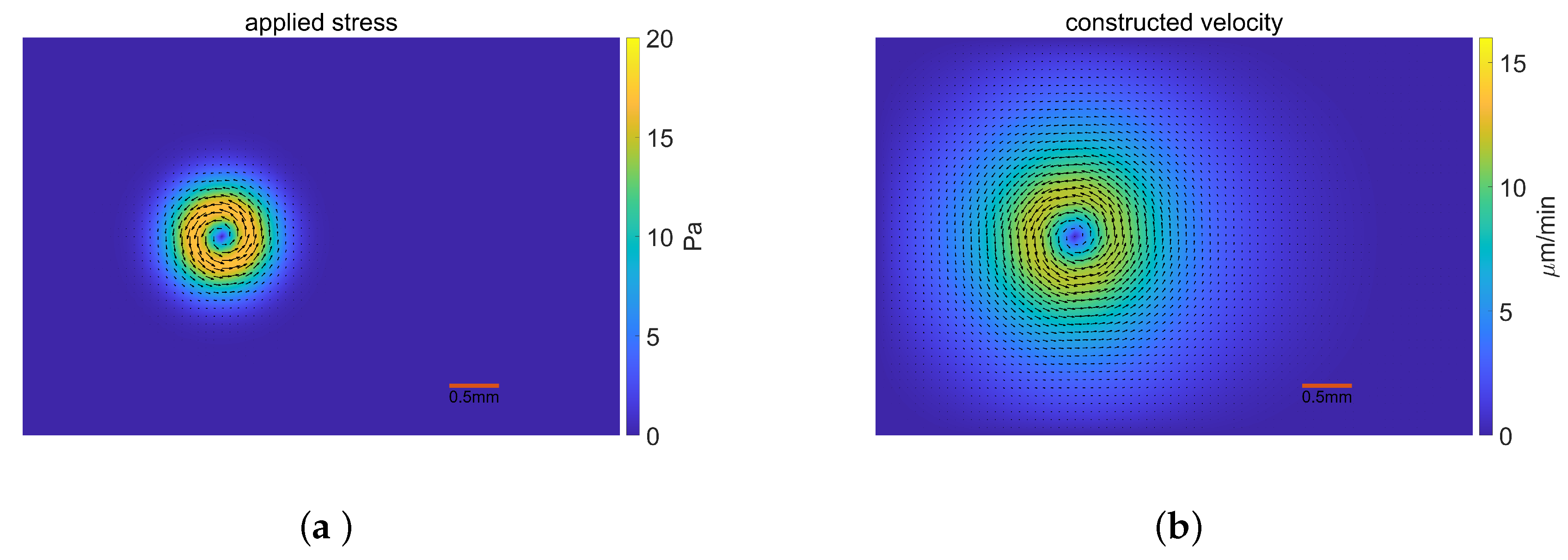
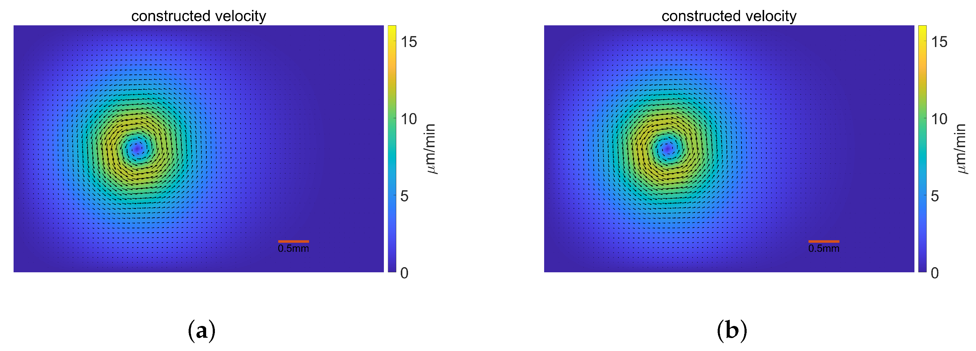
5.1. Velocity Construction

We assume a viscous Stokes flow with an approximate 2D viscosity as $50·{10}^{-1}\mathrm{k}\mathrm{g} {\mathrm{s}}^{-1}$ and moves in a rectangle domain $\Omega$ under the scale of micrometer. We assume the velocity on the boundary as 0. Then, the incompressible Stokes fluid equations are written as Equation (75):

$$\left\{\begin{array}{cc}-50·{10}^{-1}△\mathbf{u}+▽p=\mathbf{f},\hfill & \mathrm{in}\Omega ,\hfill \\ ▽·\mathbf{u}=0,\hfill & \mathrm{in}\Omega ,\hfill \\ \mathbf{u}=0,\hfill & \mathrm{on}\Gamma .\hfill \end{array}\right.$$

(75)

We apply the stress $\overline{\mathbf{f}}$ (76, 77) shown in Figure 1a and construct the fluid velocity field shown in Figure 1b.

$$\overline{\mathbf{f}}=({\overline{\mathbf{f}}}_1,{\overline{\mathbf{f}}}_2),$$

(76)

where

$$\left\{\begin{array}{c}{\overline{\mathbf{f}}}_1=1·{10}^{-1}·(y-2000)·e^{-[{\displaystyle \frac{{(x-2000)}^2}{{400}^2}}+{\displaystyle \frac{{(y-2000)}^2}{{400}^2}}]},\\ {\overline{\mathbf{f}}}_2=-1·{10}^{-1}·(x-2000)·e^{-[{\displaystyle \frac{{(x-2000)}^2}{{400}^2}}+{\displaystyle \frac{{(y-2000)}^2}{{400}^2}}]}.\end{array}\right.$$

(77)

Figure 1. The applied stress distribution and the constructed velocity field. (a) The applied stress; (b) The constructed velocity.

Before starting the inverse procedure, we do the non-dimensionalization and derive the Reynolds number as $Re={10}^{-17}$, which is extreme small. Additionally, we set the dimensionless penalty parameter ${ϵ}^{*}$ as ${10}^{-6}$ with the initial guess of stress ${\mathbf{f}}_0$ as 0.

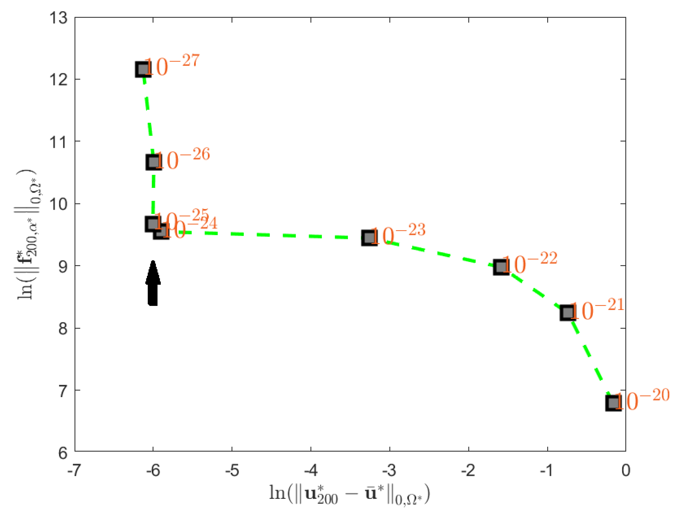
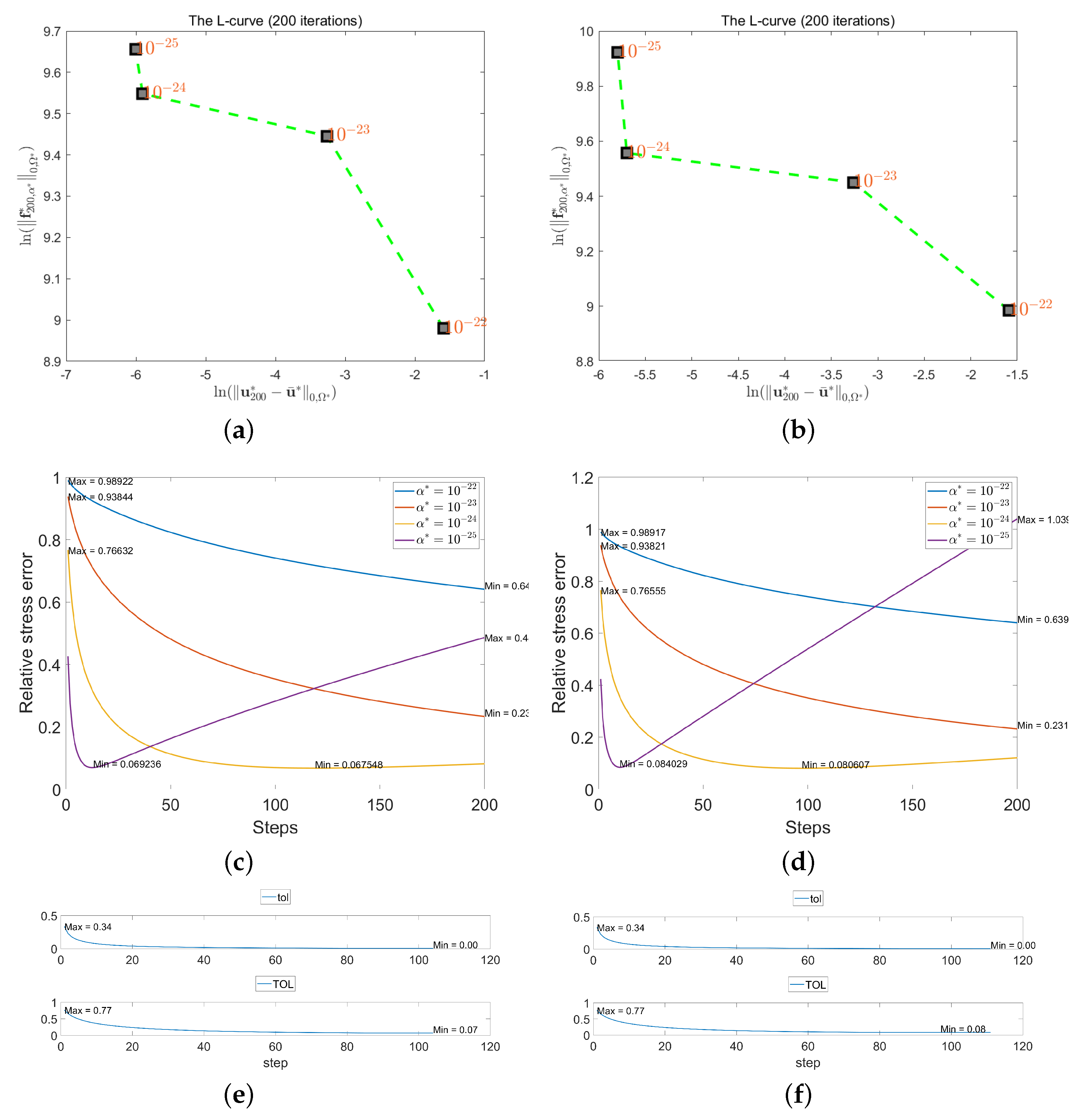
5.2. Determination of the Regularization Parameter

A number of regularization parameter choice methods have been developed to choose an optimal regularization parameter, and the most widely known methods among them are the Morozov discrepancy principle method (MDP), generalized cross-validation method (GCV) and L-curve method [5,25]. Most of these methods have been developed with their analytical justification. Morozov discrepancy principle method has the advantages of its theoretical robustness but it requires prior information on the noise of measured data accurately [26,27]. The GCV and L-curve are well-known heuristic methods for choosing the regularization parameter but do not guarantee the famous “Bakushinskii Veto”, which may lead to the failure of the regularization in some cases [28]. GCV is widely applied in practical applications as it performs very well for moderately large data set that contain white noise. However, it will be rather unstable for smaller data or data with colored noise [29]. The L-curve method is popular for its simplicity and intuitive appeal, and leads to a very reliable estimation of the regularization parameter in most practical applications [30]. However, it needs heavy computation and non-convergence when the noise level in the measurements tends to zero.

The L-curve was first applied by Lawson and Hanson in 1974 [31] and developed by Hansen and O’Leary [32]. While critics of the L-curve method due to its lack of theoretical robustness. Hanke confirmed the theoretical flaws of L-curve including failure for high-smooth/low-noise data, the parameter’s decay too quickly resulting in non-convergence [33]. While they also indirectly acknowledged L-curve’s practical value such as no prior noise required, computationally efficient, suitable for non-smooth solution/medium noise scenarios. He concluded the feasibility of L-curve that it can still be used in specific problems (e.g., live imaging and non-smooth solutions) [33]. Later, Hansen pointed that it makes sense to develop and use parameter-choice methods as a heuristic strategy for finite-dimensional ill-posed problems with bounded noise data. Additionally, in many important applications, the norm of the error in the given right-hand side is not explicitly known, which also promotes the investigations of the L-curve dealing with practical inverse problems [25]. Rezghi introduced a new variant of the L-curve for Tikhonov regularization, demonstrating its effectiveness in selecting optimal parameters for discrete ill-posed problems, particularly for those with smooth solutions, and comparing its performance with the traditional L-curve through numerical experiments [34].

Additionally, considerable computational experience indicates that the L-curve criterion is a powerful method for determining a suitable regularization parameter for many problems of interest in science and engineering, such as in electrical resistance tomography (ERT) [35] and geoid gradient components estimation [36]. Calvetti proved that the iterative method can efficiently determine the L-curve-optimal Tikhonov regularization parameter for large-scale ill-posed problems, enabling robust regularization without prior noise knowledge and demonstrating practical effectiveness through numerical examples in the reconstruction of X-ray images [37]. Johnston evaluated and demonstrated the superior performance of two L-curve corner selection methods in Tikhonov regularization for ill-posed inverse problems in electrocardiography, particularly under correlated geometry noise [38]. Our model is proposed for solving practical fluid inverse problems, the noise level of measured data are not available. We chose L-curves as the empirical regularization parameter determination approach in our model in light of this situation, as well as the effective performance of the L-curves in the advancement of current L-curve research and real-world applications. The L-curve is the plot of

$$\left(ln{∥{\mathbf{u}}_N^{*}-{\overline{\mathbf{u}}}^{*}∥}_{0,{\Omega }^{*}},ln{∥{\mathbf{f}}_{N,{\alpha }^{*}}^{*}∥}_{0,{\Omega }^{*}}\right)$$

(78)

as the regularization parameter ${\alpha }^{*}$ varies. The corner of the L-curve will indicate the proper regularization parameter ${\alpha }^{*}$. We set 200 iterations and have performed eight times of the iterative inverse procedure by selecting ${\alpha }^{*}$ as ${10}^{-20},{10}^{-21},\cdots ,{10}^{-27}$ and plot the L-curve in Figure 2. The corner of the L-curve indicates that the proper ${\alpha }^{*}$ is ${10}^{-24}$.

Figure 2. The L-curve for the SIM validation.

To identify the accuracy of the numerical results as ${\alpha }^{*}$ varies, we define the relative stress error $TOL$, the numerical velocity error $tol$ and the reconstructed velocity error $Tol$ in (79):

$$\begin{array}{c}TOL={\displaystyle \frac{{∥{\mathbf{f}}_n^{*}-{\overline{\mathbf{f}}}^{*}∥}_{0,{\Omega }^{*}}}{{∥{\overline{\mathbf{f}}}^{*}∥}_{0,{\Omega }^{*}}}}={\displaystyle \frac{\sqrt{{\int }_{{\Omega }^{*}}|{({\mathbf{f}}_n^{*}-{\overline{\mathbf{f}}}^{*})}_1^2+{({\mathbf{f}}_n^{*}-{\overline{\mathbf{f}}}^{*})}_2^2|\mathrm{d}{\mathbf{x}}^{*}}}{\sqrt{{\int }_{{\Omega }^{*}}|{\overline{\mathbf{f}}}_1^{*2}+{\overline{\mathbf{f}}}_2^{*2}|\mathrm{d}{\mathbf{x}}^{*}}}}\\ \\ tol={\displaystyle \frac{{∥{\mathbf{u}}_n^{*}-{\overline{\mathbf{u}}}^{*}∥}_{0,{\Omega }^{*}}}{{∥{\overline{\mathbf{u}}}^{*}∥}_{0,{\Omega }^{*}}}}={\displaystyle \frac{\sqrt{{\int }_{{\Omega }^{*}}|{({\mathbf{u}}_n^{*}-{\overline{\mathbf{u}}}^{*})}_1^2+{({\mathbf{u}}_n^{*}-{\overline{\mathbf{u}}}^{*})}_2^2|\mathrm{d}{\mathbf{x}}^{*}}}{\sqrt{{\int }_{{\Omega }^{*}}|{\overline{\mathbf{u}}}_1^{*2}+{\overline{\mathbf{u}}}_2^{*2}|\mathrm{d}{\mathbf{x}}^{*}}}}\\ \\ Tol={\displaystyle \frac{{∥{\mathbf{u}}_{re}^{*}-{\overline{\mathbf{u}}}^{*}∥}_{0,{\Omega }^{*}}}{{∥{\overline{\mathbf{u}}}^{*}∥}_{0,{\Omega }^{*}}}}={\displaystyle \frac{\sqrt{{\int }_{{\Omega }^{*}}|{({\mathbf{u}}_{re}^{*}-{\overline{\mathbf{u}}}^{*})}_1^2+{({\mathbf{u}}_{re}^{*}-{\overline{\mathbf{u}}}^{*})}_2^2|\mathrm{d}{\mathbf{x}}^{*}}}{\sqrt{{\int }_{{\Omega }^{*}}|{\overline{\mathbf{u}}}_1^{*2}+{\overline{\mathbf{u}}}_2^{*2}|\mathrm{d}{\mathbf{x}}^{*}}}}\end{array}$$

(79)

The stress errors $TOL$ regarding to different choices of ${\alpha }^{*}$ are depicted in Figure 3 and Figure 4. We found that $TOL$ could reach to $0.07$ only when ${\alpha }^{*}$ is ${10}^{-24}$ or ${10}^{-25}$. Even while the stress error quickly drops to zero at ${\alpha }^{*}={10}^{-25}$, it then rises significantly. Thus, it confirms that the proper ${\alpha }^{*}$ is ${10}^{-24}$ as the error reaches its minimum and tends to be stabilize after that.

Figure 3. The relative stress error regarding to different ${\alpha }^{*}$.

Figure 4. The relative stress error regarding to two different ${\alpha }^{*}$.

Then, we do the inverse procedure with the determined proper regularization parameter ${10}^{-24}$ after setting the stopping criterion as the relative velocity error $tol<0.005$. It then takes 104 iterations to derive the results. We plot the convergence performance when ${\alpha }^{*}$ is ${10}^{-24}$ in Figure 5. In the first 25 iterations or so, $tol$ also drops quickly and steadily becomes less. During whole iterations, the magnitude of $tol$ falls from ${10}^{-1}$ to ${10}^{-3}$. For the relative stress error $TOL$, it rapidly declines and reaches to its minimum. The magnitude of $TOL$ drops from ${10}^{-1}$ to ${10}^{-2}$ during whole process. The computed stress error confirms that the model is accurate and stable when ${\alpha }^{*}={10}^{-24}$.

Figure 5. The convergence performance.

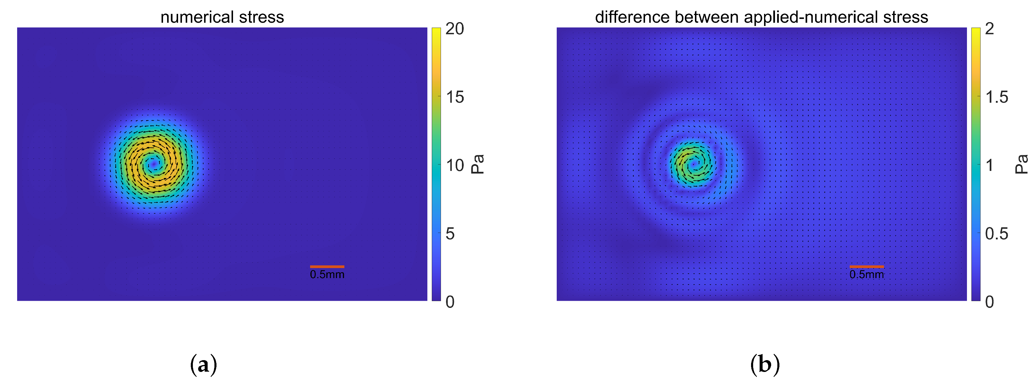
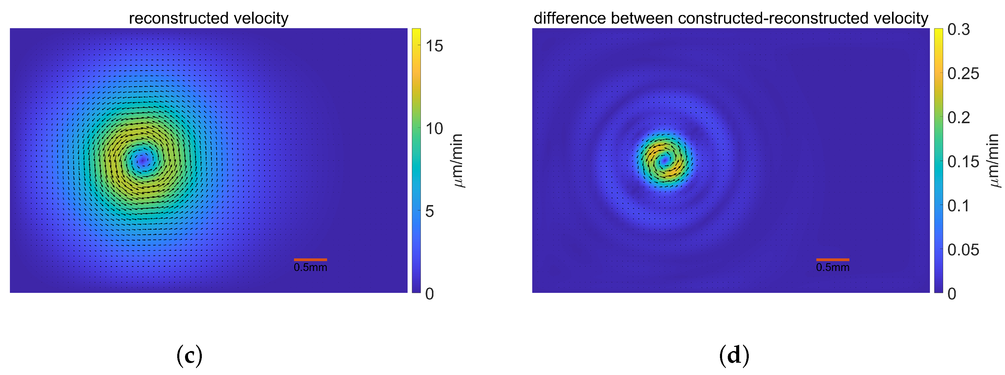
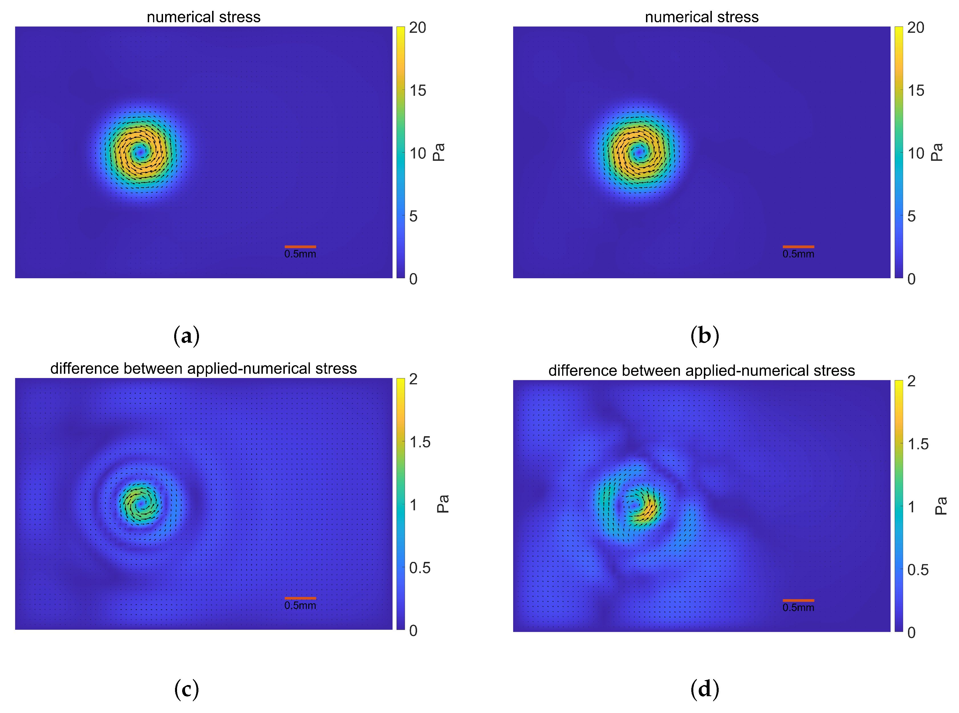
5.3. Model Validation Results

We present the results for the SIM validation depicted in Figure 6. The numerical stress distribution in Figure 6a has a quite similar pattern as the given stress. In general, the stress error is dispersed and the error magnitude is less than $1\mathrm{Pa}$ in Figure 6b. A small portion of the area where stresses are primarily distributed has an inaccuracy that is more noticeable, at a magnitude less than $2\mathrm{Pa}$. The velocity field reconstructed by the numerical stress distribution in Figure 6c and the constructed velocity field are almost identical. The area where the velocity mainly dispersed is where the difference mostly concentrated, with a variation of less than $0.3\mu \mathrm{m} {\min }^{-1}$ among $10\mu \mathrm{m} {\min }^{-1}$ shown in Figure 6d. Given that the numerical results more closely resemble the given stress in the model validation, the SIM performs reasonably well.

Figure 6. Validation results for the Stationary Incompressible SIM under iterative Tikhonov regularization. (a) The numerical stress; (b) The difference between the applied and the numerical stress; (c) The reconstructed velocity; (d) The difference between the constructed and the reconstructed velocity.

5.4. Model Validation for Perturbed Velocities

Finally, we discuss the stability of the model for perturbed velocity data. The constructed velocities were affected by randomly produced noise on magnitudes of $\delta$, which are $0.1\%$ Figure 7a and $1\%$ Figure 7b, respectively. The perturbed velocities are shown in Figure 7.

Figure 7. The perturbed constructed velocity fields. (a) The constructed velocity perturbed by $0.1\%$ noise; (b) The constructed velocity perturbed by $1\%$ noise.

With the given data noise level, it is theoretically reasonable to determine the appropriate regularization parameters by MDP. So, we conducted the validation of the results with the proper ${\alpha }^{*}$ derived from MDP. We developed the self-adaptive algorithm to determine proper ${\alpha }^{*}$ satisfying the MDP residual norm constraint in every Tikhonov iteration and derive the optimal iterative result. In every iteration, the MDP leads to different ${\alpha }^{*}$ and the numerical errors are stable after several iterations. We recorded the iteration numbers when the velocity error starts to be stable and the corresponding ${\alpha }^{*}$ in the following Table 2. For data with $0.1\%$ noise, it takes 7 iterations to reaches the minimum stress error $10.57\%$ when ${\alpha }^{*}$ is $2.64392\times {10}^{-21}$ and for data with $1\%$ noise, it takes 12 iterations to reaches the minimum stress error $0.373748$ when ${\alpha }^{*}$ is $7.27247\times {10}^{-23}$.

Table 2. Numerical errors for the perturbed velocity from MDP.

Noise Level	Proper ${\mathit{\alpha }}^{*}$	Iterations	Stress Error	Numerical Velocity Error	Reconstructed Velocity Error
$0.1\%$	$2.6·{10}^{-21}$	7	$10.57\%$	$0.9\%$	$0.9\%$
$1\%$	$7.3·{10}^{-23}$	12	$37.37\%$	$8.99\%$	$8.99\%$

We also validate the SIM using L-curve for proper ${\alpha }^{*}$ determination. The corner of the L-curve indicates that the proper ${\alpha }^{*}$ are ${10}^{-24}$ for above two validations shown in Figure 8a,b, which are confirmed by the relative stress error performance shown in Figure 8c,d. By setting the stopping criterion $tol<0.005$ for both validations, the errors are summarized in Table 3.

Figure 8. The L-curve and convergence performance for perturbed velocity. (a) The L-curve for velocity with $0.1\%$ noise; (b) The L-curve for velocity with $1\%$ noise; (c) The relative stress error for velocity with $0.1\%$ noise; (d) The relative stress error for velocity with $1\%$ noise; (e) The convergence performance for velocity with $0.1\%$ noise when ${\alpha }^{*}={10}^{-24}$; (f) The convergence performance for velocity with $1\%$ noise when ${\alpha }^{*}={10}^{-24}$.

Table 3. Numerical errors for the perturbed velocity from L-curve.

Noise Level	Proper ${\mathit{\alpha }}^{*}$	Iterations	Stress Error	Numerical Velocity Error	Reconstructed Velocity Error
$0.1\%$	${10}^{-24}$	104	$6.9\%$	$0.49\%$	$0.49\%$
$1\%$	${10}^{-24}$	111	$8.2\%$	$0.49\%$	$0.47\%$

For perturbed velocity with $0.1\%$ noise level, it takes 104 iterations and $TOL$ reaches to $0.069$ in the end. For perturbed velocity with $1\%$ noise level, it takes 111 iterations and $TOL$ reaches to $0.082$ in the end. From both convergence performance, we find that $tol$ drops quickly in the first 25 iterations or so, and steadily becomes less when ${\alpha }^{*}$ is ${10}^{-24}$ shown in Figure 8e,f. During whole iterations, the magnitude of $tol$ falls from ${10}^{-1}$ to ${10}^{-3}$. The relative stress error $TOL$ rapidly declines in the first 20 iterations and steadily becomes less. The magnitude of $TOL$ drops from ${10}^{-1}$ to ${10}^{-2}$ during whole process.

The MDP gives higher ${\alpha }^{*}$ and takes less iterations to derive its optimal solution than L-curve. Unlike the ${\alpha }^{*}$ change as iterations in MDP, the ${\alpha }^{*}$ determined at the inflection point of the L-curve are used for each iteration. Through the comparison of the error results between the MDP and L-curve, we noticed that numerical stress distributions and the reconstructed velocity fields are more accurate through L-curve for the same noise data. Additionally, the noise level increases from $0.1\%$ to $1\%$, the errors do not change too much in the L-curve, while the inverse occurs for MDP. This indicates that the determining ${\alpha }^{*}$ through the L-curve is less susceptible to interference from noise levels compared to MDP. The possible reasons that the L-curve performs well in this problem might be that the data in our validation are finite-dimensional through region segmentation and the noise level is bounded, but the theoretical analysis for rigorous error-controlled regularization needs to be clarified in the future. So, we then employed the proper ${\alpha }^{*}$ derived from the L-curve and presented the corresponding results in Figure 9 and provides the results for $0.1\%$ noise perturbed data on the left column and $1\%$ noise data on the right. Both numerical stress distributions are shown in Figure 9a, and Figure 9b has a quite similar pattern as the applied stress. The area where the stress is mainly dispersed is where the difference is mostly concentrated, at a magnitude less than $2\mathrm{Pa}$ among $20\mathrm{Pa}$ in Figure 9c. The numerical stress for $1\%$ noise has no significant deviation from the given force, the error is still within $2\mathrm{Pa}$ in Figure 9d. The velocity field reconstructed by the numerical stress distribution and the constructed velocity field are almost identical. For $0.1\%$ noise level, it has a smooth variation of less than $0.3\mu \mathrm{m} {\min }^{-1}$ among $10\mu \mathrm{m} {\min }^{-1}$, as shown in Figure 9e, while the variation is less smooth for data with $1\%$ noise level in Figure 9f. This work indicates the model’s stability for certain perturbed data.

Figure 9. Validation results for perturbed velocity. (a) The numerical stress for velocity with $0.1\%$ noise; (b) The numerical stress for velocity with $1\%$ noise; (c) The difference between the applied and the numerical stress for velocity with $0.1\%$ noise; (d) The difference between the applied and the numerical stress for velocity with $1\%$ noise; (e) The difference between the consturcted and the reconstructed stress for velocity with $0.1\%$ noise; (f) The difference between the consturcted and the reconstructed stress for velocity with $1\%$ noise.

6. Conclusions

In this paper, we propose and develop a Stokes Inverse Model (SIM) to estimate the stresses from the velocity data. We tackle the inverse problem governed by the Stokes equations constraining the solutions using iterative Tikhonov (IT) regularization. After the model formulation, we validate the model for non-perturbed and perturbed synthetic data and derive reliable stress distributions that are sufficiently robust to reconstruct the velocity fields close to those constructed velocities. The proper regularization parameter is effectively identified using the L-curve criterion, resulting in stable convergence and precise results. The effectiveness of L-curve criterion for regularization parameter determination has been verified in the model. But as a heuristic strategy, the theoretical analysis for rigorous error-controlled regularization needs to be clarified in the future.

The proposed SIM provides a complete framework for stress estimation using IT regularization; however, its inherent theoretical and computational limitations still constrain its practical applicability. The linear Stokes framework neglects nonlinear effects and transient, viscoelastic behaviors critical to biological systems. Simplified 2D geometries with homogeneous Dirichlet boundaries further limit real-world utility, as complex 3D domains and inhomogeneous boundary conditions remain unaddressed. Computationally, the finite element method is computationally prohibitively expensive for 3D systems because of cubic growth in degrees of freedom and the lack of adaptive mesh refinement (AMR) to effectively resolve high-gradient regions. Although the verification of synthetic data are effective, in practical applications, the accuracy of the model will be challenged due to the errors caused by experimental noise and incomplete spatial coverage, and the heuristic L-curve parameter selection lacks a theoretical guarantee for complex or noisy scenarios.

In order to improve the applicability of the proposed model, future work should prioritize extending to nonlinear regimes, such as compressible Navier–Stokes flows, and transient problems incorporating adaptive mesh strategies to mitigate computational costs. Assessing robustness under realistic noise and sparse measurements requires experimental validation using real-world data, such as particle image velocimetry (PIV) from biological records or offshore platforms. Reliability may be increased by strengthening regularization strategies to manage non-Gaussian or spatially correlated noise in conjunction with strict parameter selection standards. Additionally, investigating parallel computing architectures might increase the range of applications that can be used in 3D. The SIM framework can develop into a flexible instrument for stress estimation in intricate biological and engineering systems by filling in these gaps.

References

- Lekka, M.; Gnanachandran, K.; Kubiak, A.; Zieliński, T.; Zemła, J. Traction force microscopy—Measuring the forces exerted by cells. Micron 2021, 150, 1–9. [Google Scholar] [CrossRef] [PubMed]
- Zhang, J.; Rothenberger, S.M.; Brindise, M.C.; Markl, M.; Rayz, V.L.; Vlachos, P.P. Wall Shear Stress Estimation for 4D Flow MRI Using Navier-Stokes Equation Correction. Ann. Biomed. Eng. 2022, 50, 1810–1825. [Google Scholar] [CrossRef] [PubMed]
- Chen, J.; Raiola, M.; Discetti, S. Pressure from data-driven estimation of velocity fields using snapshot PIV and fast probes. Exp. Therm. Fluid Sci. 2022, 136, 1–13. [Google Scholar] [CrossRef]
- Kabanikhin, S. Definitions and examples of inverse and ill-posed problems. J. Inverse -Ill-Posed Probl. 2008, 16, 317–357. [Google Scholar] [CrossRef]
- Kirsch, A. An Introduction to the Mathematical Theory of Inverse Problems; Springer: Cham, Switzerland, 1996. [Google Scholar]
- Siraj-ul-Islam; Ahsan, M.; Hussian, I. A multi-resolution collocation procedure for time-dependent inverse heat problems. Int. J. Therm. Sci. 2018, 128, 160–174. [Google Scholar] [CrossRef]
- Tikhonov, A.N. On the solution of ill-posed problems and the method of regularization. Dokl. Akad. Nauk. Sssr 1963, 151, 501–504. [Google Scholar]
- Li, M.; Wang, L.; Luo, C.; Wu, H. A new improved fractional Tikhonov regularization method for moving force identification. Structures 2024, 60, 1–15. [Google Scholar] [CrossRef]
- Lauga, E.; Powers, T.R. The Hydrodynamics of Swimming Microorganisms. Rep. Prog. Phys. 2009, 72, 1–52. [Google Scholar] [CrossRef]
- Nashed, M.Z. The theory of Tikhonov regularization for Fredholm equations of the first kind (C. W. Groetsch). Siam Rev. 1986, 28, 116–118. [Google Scholar] [CrossRef]
- Kryanev, A.V. An iterative method for solving incorrectly posed problems. Ussr Comput. Math. Math. Phys. 1974, 14, 24–35. [Google Scholar] [CrossRef]
- Engl, H.W.; Hanke, M.; Neubauer, A. Regularization of Inverse Problems; Kluwer Academic Publishers: Dordrecht, The Netherlands, 1996. [Google Scholar]
- Vainikko, G.M.; Veretennikov, A.Y. Iteration Procedures in Ill-Posed Problems; Nauka: Moscow, Russia, 1986. [Google Scholar]
- Gerth, D. A new interpretation of (Tikhonov) regularization. Inverse Probl. 2021, 37. [Google Scholar] [CrossRef]
- Hanke, M.; Groetsch, C. Nonstationary iterated Tikhonov regularization. J. Optim. Theory Appl. 1998, 98, 37–53. [Google Scholar] [CrossRef]
- Chang, W.; D’Ascenzo, N.; Xie, Q. A relaxed iterated tikhonov regularization for linear ill-posed inverse problems. J. Math. Anal. Appl. 2024, 530. [Google Scholar] [CrossRef]
- White, F.M.; Hess, J.L.; Gibson, C.H. Equations for Fluid Statics and Dynamics. In Handbook of Fluid Dynamics and Fluid Machinery; Wiley: Hoboken, NJ, USA, 1996; pp. 1–90. [Google Scholar]
- Nakayama, Y. Chapter 10—dimensional analysis and law of similarity. In Introduction to Fluid Mechanics, 2nd ed.; Butterworth-Heinemann: Oxford, UK, 2018; pp. 203–214. [Google Scholar]
- Durbin, P.A.; Medic, G. Creeping flow. In Fluid Dynamics with a Computational Perspective; Cambridge University Press: Cambridge, UK, 2007; pp. 108–131. [Google Scholar]
- Mathé, P.; Hofmann, B. How general are general source conditions? Inverse Probl. 1993, 24, 015009. [Google Scholar]
- Temam, R. Une méthode d’approximation de la solution des équations de navier-stokes. Bull. Soc. Math. Fr. 1968, 96, 115–152. [Google Scholar] [CrossRef]
- Lin, P. A sequential regularization method for time-dependent incompressible navier-stokes equations. Siam J. Numer. Anal. 1997, 34, 1051–1071. [Google Scholar] [CrossRef]
- Hecht, F. New development in freefem++. J. Numer. Math. 2012, 20, 251–265. [Google Scholar] [CrossRef]
- Gao, Y. Developing Stokes Inverse Models that Estimate Stresses Driving Tissue Flows during Gastrulation in Chick Embryos; University of Dundee: Dundee, UK, 2023. [Google Scholar]
- Hansen, P.C. Rank-Deficient and Discrete Ill-Posed Problems: Numerical Aspects of Linear Inversion; Society for Industrial and Applied Mathematics (SIAM): Philadelphia, PA, USA, 1998. [Google Scholar]
- Morozov, V.A. Regularization of incorrectly posed problems and the choice of regularization parameter. Ussr Comput. Math. Math. Phys. 1966, 6, 242–251. [Google Scholar] [CrossRef]
- Engl, H.W. Discrepancy principles for Tikhonov regularization of ill-posed problems leading to optimal convergence rates. J. Optim. Theory Appl. 1987, 52, 209–215. [Google Scholar] [CrossRef]
- Bakushinskii, A.B. Remarks on choosing a regularization parameter using the quasi-optimality and ratio criterion. USSR Comput. Math. Math. Phys. 1984, 24, 181–182. [Google Scholar] [CrossRef]
- Fenu, C.; Reichel, L.; Rodriguez, G. GCV for Tikhonov regularization via global Golub–Kahan decomposition. Numer. Linear Algebra Appl. 2016, 23, 467–484. [Google Scholar] [CrossRef]
- Hansen, P.C. Analysis of discrete ill-posed problems by means of the L-curve. Siam Rev. 1992, 34, 561–580. [Google Scholar] [CrossRef]
- Lawson, C.L.; Hanson, R.J. Solving Least Squares Problems; Prentice-Hall: Hoboken, NJ, USA, 1974. [Google Scholar]
- Hansen, P.C.; O’Leary, D.P. The use of the L-curve in the regularization of discrete ill-posed problems. Siam J. Sci. Comput. 1993, 14, 1487–1503. [Google Scholar] [CrossRef]
- Hanke, M. Limitations of the L-curve method in ill-posed problems. Bit Numer. Math. 1996, 36, 287–301. [Google Scholar] [CrossRef]
- Rezghi, M.; Hosseini, S.M. A new variant of L-curve for Tikhonov regularization. J. Comput. Appl. Math. 2009, 231, 914–924. [Google Scholar] [CrossRef]
- Xu, Y.; Pei, Y.; Dong, F. An extended L-curve method for choosing a regularization parameter in electrical resistance tomography. Meas. Sci. Technol. 2016, 27, 1–6. [Google Scholar] [CrossRef]
- Yu, D.; Hwang, C.; Zhu, H.; Ge, S. The Tikhonov-L-curve regularization method for determining the best geoid gradients from SWOT altimetry. J. Geod. 2023, 97, 1–13. [Google Scholar] [CrossRef]
- Calvetti, D.S.; Morigi, S.; Reichel, L.; Sgallari, F. Tikhonov regularization and the L-curve for large discrete ill-posed problems. J. Comput. Appl. Math. 2000, 123, 423–446. [Google Scholar] [CrossRef]
- Johnston, P.R.; Gulrajani, R.M. Selecting the corner in the L-curve approach to Tikhonov regularization. IEEE Trans. Biomed. Eng. 2000, 47, 1293–1296. [Google Scholar] [CrossRef]
Disclaimer/Publisher’s Note: The statements, opinions and data contained in all publications are solely those of the individual author(s) and contributor(s) and not of MDPI and/or the editor(s). MDPI and/or the editor(s) disclaim responsibility for any injury to people or property resulting from any ideas, methods, instructions or products referred to in the content. |
© 2025 by the authors. Licensee MDPI, Basel, Switzerland. This article is an open access article distributed under the terms and conditions of the Creative Commons Attribution (CC BY) license (https://creativecommons.org/licenses/by/4.0/).