Abstract
The dynamic and uncertain nature of financial markets presents significant challenges in accurately predicting portfolio returns due to inherent volatility and instability. This study investigates the potential of logistic regression to enhance the accuracy and robustness of return classification models, addressing challenges in dynamic portfolio optimization. We propose a price-aware logistic regression (PALR) framework to classify dynamic portfolio returns. This approach integrates price movements as key features alongside traditional portfolio optimization techniques, enabling the identification and analysis of patterns and relationships within historical financial data. Unlike conventional methods, PALR dynamically adapts to market trends by incorporating historical price data and derived indicators, leading to more accurate classification of portfolio returns. Historical market data from the Dow Jones Industrial Average (DJIA) and Hang Seng Index (HSI) were used to train and test the model. The proposed scheme achieves an accuracy of 99.88%, a mean squared error (MSE) of 0.0006, and an AUC of 99.94% on the DJIA dataset. When evaluated on the HSI dataset, it attains a classification accuracy of 99.89%, an AUC of 99.89%, and an MSE of 0.011. The results demonstrate that PALR significantly improves classification accuracy and AUC while reducing MSE compared to conventional techniques. The proposed PALR model serves as a valuable tool for return classification and optimization, enabling investors, assets, and portfolio managers to make more informed and effective decisions.
Keywords:
logistic regression; dynamic portfolio optimization; return classification; machine learning; uncertainty; financial risk MSC:
91G99
1. Introduction
In recent years, the unpredictability, complexity, and uncertainty of financial markets have alarmed investors. These factors have significantly raised financial risks and market instability [1]. Thus, more concerted effort is required from researchers and investors to develop effective and efficient strategies for predicting emerging market returns and risks. Doing so will significantly mitigate the impact of catastrophic events and asset losses. The future of these markets will play a crucial role in portfolio management and investment. With rapid advancements in machine learning and optimization, new opportunities are emerging for portfolio management. These technologies can be incorporated and integrated to improve investment strategies. The goal is to maximize returns and minimize risk, especially in uncertain and rapidly changing market conditions [2]. Identifying and selecting the best asset for wealth investment requires an effective approach, strategy, and policy. A well-structured investment plan helps achieve higher returns while minimizing risk. In addition, it is important to note that assets possess distinct characteristics and qualities. These attributes vary from one asset to another. There is a dramatic need to develop a dynamic portfolio optimization scheme to adapt to market dynamics. Consequently, this requires an approach with high precision and accuracy to predict market dynamics and returns.
Portfolio optimization has seen a significant rise in usage and demand within the financial industry, as it helps maximize returns while effectively managing risk. Harry Markowitz pioneered and developed the concept of traditional portfolio optimization in the 1950s based on mean-variance optimization. This approach determines the trade-off between expected return and risk. In today’s rapidly changing and interconnected financial markets, traditional portfolio strategies struggle to adapt. They fail to account for the dynamic nature of market conditions and evolving investor preferences. Portfolio management, optimization, and resource allocation have real-world applications in areas such as transaction cost, risk, trade constraint, and asset return prediction. These techniques help investors make informed decisions by balancing risk and return while considering market constraints. Predicting future returns has been a major concern for managers in today’s financial world. This primarily involves using the model to predict short-term and long-term returns and observe the key factors affecting asset returns [3].
Dynamic portfolio optimization is a powerful strategy for managing investments in a rapidly evolving financial landscape. By continuously adjusting portfolios based on real-time data and market trends, investors can enhance returns and manage risk effectively. However, successful implementation requires overcoming challenges related to complexity, data requirements, and model uncertainty [4,5,6,7,8,9,10]. Dynamic portfolio optimization is crucial, as it significantly aids in the selection and management of assets in challenging and uncertain market conditions. It requires an efficient and strategic approach to asset and resource selection to maximize profits while minimizing risk. Market dynamics influence returns through various factors. The underutilized data collected from different financial institutions and markets can be useful in studying market dynamics and patterns. Dynamic portfolio optimization provides an effective solution to the limitations of conventional approaches. It adjusts portfolio compositions in response to changing market conditions, economic indicators, and risk preferences. Furthermore, it provides better market opportunities and risk management and enhances investment performance.
Machine-learning techniques will enable effective learning of financial data patterns [11]. They will also support and manage dynamic portfolio optimization and decision-making. In addition, there have been no studies related to the application of the logistic regression approach in dynamic portfolio optimization. This gap presents an opportunity to enhance investment strategies and improve returns. The primary aim of this study is to combine logistic regression with dynamic portfolio optimization to enhance the prediction accuracy and precision of asset returns. The proposed approach enables efficient and accurate financial predictions. This advancement makes a significant contribution to the financial industry and investment strategies. Consequently, it will save investors time and ensure effective investment decisions. The proficiency of the proposed approach has been evaluated using performance metrics based on real-world DJIA and HSI historical data. It has also been compared with other machine-learning techniques to assess its effectiveness. Therefore, we used these datasets to evaluate the consistency of the approaches across various time periods and market conditions.
This study proposes a dynamic portfolio return classification algorithm that incorporates PALR to enhance accuracy and precision. The price-aware dynamic portfolio return classification scheme for uncertain financial markets primarily uses logistic regression to classify and predict returns. It leverages market price values and dynamics to enhance predictive accuracy. The proposed scheme makes a significant contribution to the field of financial analytics and portfolio optimization and introduces an innovative approach to classifying portfolio returns, improving both accuracy and reliability. In contrast with traditional methods, PALR demonstrates an ability to dynamically adjust to changing market conditions. Ultimately, this ensures that the model remains robust and relevant across various financial environments. It effectively captures the nuances inherent in the stock market. The contributions are as follows:
- Introduces a PALR model incorporating price movements and historical financial indicators for return classification.
- Develops a mathematical framework for price deviation and market dynamics to enhance adaptability and performance.
- Achieves high performance from the proposed new approach in classifying the dynamic portfolio return in an unpredictable market environment.
- Compares the performance of the proposed PALR with traditional machine learning using DJIA and HSI historical data.
The rest of the paper is organized as follows: Section 2 focuses mainly on related works. Section 3 presents the dynamic portfolio return mathematical framework and concept and the data used. Section 4 introduces the PALR dynamic portfolio return prediction scheme. The experiments and results are discussed in Section 5. In Section 6, the summary and conclusions are presented.
2. Related Works
To examine and review related works in portfolio optimization, return, risk, and uncertainty, it is essential to explore the concepts related to dynamic portfolios and previous studies in the field. Several studies have been conducted, but only the most relevant ones will be discussed. The foundational concept of portfolio optimization was introduced by Markowitz. Since then, numerous research efforts have sought to further explore and enhance this field. In [12], the trade-off between return and risk in portfolio selection is demonstrated. Additionally, ref. [13] examines the dynamic mean-variance approach to portfolio selection, accounting for stochastic interest rates and liabilities. Furthermore, an approach for selecting a portfolio based on dynamic mean variance to critically analyze the market timing is proposed in [14].
A fuzzy-based portfolio has been proposed as an alternative tool for portfolio studies by [15]. It is reported in [16] that a portfolio for different investments can be accomplished by using a fuzzy multi-period portfolio selection approach. Similarly, ref. [17] introduces a financial portfolio selection method based on a fuzzy approach, which considers return, liquidity, and risk. In [18], a fuzzy multi-objective portfolio selection strategy integrating efficiency and higher returns is proposed and developed. A mean absolute semi-deviation and triangular fuzzy approach can be integrated into multi-period portfolio optimization to achieve optimal performance, as reported in [19]. These studies offer useful ideas for dynamic portfolio optimization, but they also have some common problems. The models are often too complex, hard to use in practice, based on fixed assumptions, and not well-tested in different market situations. Fixing these issues could make the models more useful and reliable in real-world investment.
In addition, a machine-learning approach for stock prediction has been developed and introduced into the portfolio variance mean model, as reported in [20]. In [21], a multi-period model is proposed to incorporate both market environment fluctuations and transaction costs. Ref. [22] proposes an LSTM prediction approach based on the hit ratio; it outperforms both RNN and gate recurrent approaches in terms of performance. More importantly, ref. [23] presents a hybrid deep-learning scheme for stock price prediction using Black–Litterman model inputs. Ref. [24] reports a machine-learning-based technique using the Omega portfolio and mean variance to predict daily trading investment. In summary, these studies provide useful ideas about portfolio optimization and prediction methods. However, they often miss key dynamic aspects like adjusting to market changes, including transaction costs, and updating models in real time.
Furthermore, it has been reported in [25] that different machine-learning techniques are used to predict the return for the stock exchange markets. A model based on augmentation and LSTM has been developed for predicting the stock market index, as reported in [26]. In [27], an approach for predicting financial time series using a stochastic time neural network and principal component analysis is proposed and developed. Additionally, the approach presented in [28] utilizes reinforcement learning, with a primary focus on discrete single-asset trading. In contrast, ref. [29] develops a multi-asset trading scheme that does not account for transaction costs. Although these papers use modern AI and deep learning for forecasting or trading, they do not adjust portfolio weights continuously based on changing risk and return. They also do not consider how relationships among assets change over time.
Interestingly, ref. [30] proposes a linear rebalancing rule for obtaining an optimal portfolio that uses trading constraints to determine the near-optimal solution. In [31], an approach for determining the impact of ambiguity on returns and its prediction signal is proposed. More importantly, ref. [32] proposes a scheme for selecting a portfolio in environments with multiple risk assets. Collin-Dufresne et al. [33] introduce a regime-switching approach that incorporates trading costs, volatility, and expected returns in portfolio selection. Additionally, ref. [34] introduces a continuous-time approach derived from the discrete-time model previously proposed in [35]. The impact of transaction costs on equilibrium return in continuous time is studied in [36]. These studies often rely on simple assumptions like fixed rebalancing rules and predictable returns, which do not reflect real market conditions. Many also ignore factors like liquidity shocks and market friction, making them less useful for dynamic portfolio optimization.
A CNN-LSTM model with high performance capability has been developed to capture the spatial and temporal features of stock market data, as reported in [37]. In [38], a method that accounts for both volatility and noise in financial time series data to predict stock prices is proposed. In addition, ref. [39] proposes a hybrid scheme to improve prediction performance by utilizing the strengths of CNN and bidirectional LSTM. Furthermore, ref. [40] proposes a cost-sensitive scheme that assigns varying costs to different types of prediction errors, resulting in higher prediction accuracy. In [41], it is demonstrated that high-frequency predictions can be achieved by extracting features using a deep neural network informed by prior knowledge. In contrast, ref. [42] proposes a scheme for predicting stock market indices and indicators without prior knowledge. Furthermore, ref. [43] proposes an approach that simultaneously correlates and predicts multiple time series of financial data. These articles use deep learning to effectively predict financial trends. However, they do not focus on dynamic portfolio optimization, such as managing risk, allocating assets, or building performance-driven portfolios based on their forecasts.
We also reviewed studies that applied ensemble-learning techniques in finance. Son et al. [44] show that XGBoost is effective for identifying key factors in predicting company bankruptcy. Qian et al. [45] use models like AdaBoost, XGBoost, Random Forest, and GBDT to predict financial distress in Chinese firms. In [46], a new model combines ARMA with CNN-LSTM to capture both linear and nonlinear patterns in financial data. The study in [47] uses regression tree-based ensemble learning for portfolio valuation and risk management. In [48], ensemble learning is applied to imbalanced data to predict financial distress. Study [49] introduces a blending ensemble method using recurrent neural networks for stock prediction. Lastly, ref. [50] uses ensemble methods with Empirical Mode Decomposition (EMD) to improve forecasting of financial products. These articles mainly focus on predicting financial distress, bankruptcy, and stock prices. However, they do not address dynamic portfolio optimization, as they ignore changing market risks and do not adjust portfolio weights over time.
3. Materials and Methods
3.1. Data Analysis and Description
The return predictability depends greatly on the market conditions over time. Market conditions are most accurately classified in stable environments. In this work, we used DJIA and HSI financial market data for the development and testing of the proposed scheme. The DJIA and HSI are indispensable tools in financial research due to their roles as economic indicators and their influence on global markets. They also serve as essential instruments for risk assessment and performance benchmarking. These indices have been used in the development and evaluation of investment algorithms aimed at optimizing portfolio returns while managing risk [51,52]. Their effective use enhances the understanding of market behaviors and informs investment strategies. We used the two datasets (DJIA and HSI) in our study to assess whether the findings remain consistent across different periods. More importantly, using different time windows helps capture changes in trends or patterns over short-term and long-term periods. To track the market condition, daily financial market prices were used to constantly monitor market deviation.
The DJIA comprises 30 companies that represent various sectors of the economy. More importantly, the DJIA is one of the oldest and most widely followed stock market indices in the world, serving as a benchmark for overall market performance. This study mainly uses the daily transaction data of traded stocks based on the DJIA from 20 January 1992, to 18 September 2024. While the Hang Seng is the key stock market index in Hong Kong, it serves as a benchmark for the performance of the overall Hong Kong stock market. This study considered the Hang Seng stocks dataset from 7 September 2001, to 19 September 2024. More importantly, the datasets were obtained from Yahoo Finance (https://finance.yahoo.com (accessed on 21 September 2024)).
The DJIA dataset consists of 8227 records, representing daily historical data from January 1992 to September 2024. Meanwhile, 5709 records from September 2001 to September 2024 were used to examine the Hang Seng market. These two datasets differ significantly in average return, price, and deviation. This difference serves as an effective measure for evaluating the proficiency of classifiers. The daily price fluctuations clearly demonstrated the market’s dynamics over the period during which prices and returns were studied. Therefore, this indicates the suitability of the datasets, since the characteristics of the DJIA and HSI datasets reflect a typical real-world case scenario.
In addition, it is important to note that calculating financial market returns or profitability involves understanding the appreciation or depreciation of a financial asset. This process typically focuses on how much an asset, such as a stock or index, has changed in value over a specific period. The two most common measures are simple return (often called total return) and logarithmic return [53,54]. The formula to calculate the simple return for an asset over a given period (usually daily, weekly, or annually) is as follows:
where close price (Pt+1) is the market price at the end of the day and open price (Pt) is the market price at the beginning of the day. In this work, the daily financial market price has been considered to critically examine the market uncertainty. Undoubtedly, others use the logarithmic return instead of the one described in Equation (1). Hence, the logarithmic return () can be computed using Equation (2), as shown below:
Alternatively, the asset return in Equation (2) can be expressed in terms of the predictive variable (Ft) and turbulence factor (), as represented in Equation (3) below:
The function g (Ft, ωt+1) can take a linear or non-linear form and is primarily defined by two components: Ft and ωt+1. Here, Ft represents the information set available at time t, typically based on past prices, and serves as a predictive price factor. More importantly, it represents a vector of selected market indicators and technical variables known to influence asset returns. In contrast, ωt+1 denotes the shocks or innovations that occur between time t and t + 1, which may include randomness, news events, uncertainty, or market turbulence. Thus, the asset return from time t to t + 1 is modeled as a function of both the known information at time t and the unforeseen shock that follows.
To effectively determine whether a return reflects a gain or loss, we introduced a threshold into the proposed scheme. This approach significantly aided in accurately characterizing the return. Mathematically, the return characterization (RC) can be described by Equation (4), and it is represented as follows:
Stock market deviation has been used to measure the rate at which stock prices increase or decrease for a given set of returns. It is a measure of the degree of variation in stock prices over time. This makes it a useful tool for assessing the level of risk or uncertainty in the market. Tracking stock market volatility can be accomplished through key indices, technical indicators, market trends, economic reports, and real-time market data. In this study, we used standard deviation to measure the price fluctuations relative to average price. We chose to measure market volatility using standard deviation because it provides a quantifiable and widely accepted metric for understanding price fluctuations [55,56]. In essence, it plays an integral role in tracking the price fluctuations and classifying returns. A higher standard deviation indicates greater volatility, while a lower standard deviation suggests stability. The mathematical expression used for computing the standard deviation is as follows:
where
= standard deviation (market volatility);
N = number of observations (e.g., days);
ri = return of the asset/index on day I;
μ = mean return over N days, and it is given by
3.2. Dynamic Portfolio Return Mathematical Framework
The Markowitz portfolio problem can be represented mathematically to illustrate the relationship between different parameters, risk, and return. This will be crucial in developing the dynamic portfolio framework and the core concept of the portfolio optimization problem. Specifically, the impact of different parameters on risk and return can be critically analyzed and evaluated. Furthermore, the dynamics of portfolio returns in relation to uncertainty and volatility will be analyzed before deploying the classifiers to categorize market conditions. To accomplish this, let us assume we have more than two risky assets to invest in (n ≥ 2), and the investment is made over the period T.
The dynamic portfolio model focuses on identifying the portfolio that maximizes expected return in markets characterized by high risk and uncertainty. This approach accounts for market dynamics and volatility to adapt to changing conditions. The mathematical concept used is represented as follows:
Subject to
w is the vector representing the asset weight, and Δ represents the deviation matrix. Each row in the deviation matrix corresponds to time, and each column shows the deviation in each index. ∑ is the covariance matrix, and it can be computed as (ΔTΔ)/(N − 1). It is crucial to identify the most efficient portfolios that offer the highest possible return for a given level of risk.
The portfolio optimization problem can be simplified using the Lagrangian function. The Lagrangian function is essential for portfolio optimization because it allows us to solve constrained optimization problems. The Lagrangian function converts a constrained optimization problem into an unconstrained one by incorporating the constraints into the objective function using Lagrange multipliers. In addition, it combines risk minimization and return constraints into a single function. Mathematically, Equation (7) can be represented in the form of a Lagrangian function as follows:
where λ is the Lagrange multiplier for the expected return constraint, represents the Lagrange multiplier for the budget constraint, and 1 is an n-dimensional vector of ones; it ensures that the sum of weights is 1. We take the partial derivatives of Equation (9) and set each to zero. Hence, it yields the following:
Initially, we differentiate with respect to w.
In addition, Equation (7) can be differentiated further with respect to λ and γ as illustrated below:
Taking the derivatives with respect to w and setting them to zero eventually yields the optimal weight, as can be seen in Equation (10), shown below:
Equation (10) illustrates how portfolio weights change dynamically toward the optimal solution. This derivation shows that Markowitz portfolio optimization can be solved using the Lagrangian method, and its dynamic behavior can be modeled with a first-order differential equation. Furthermore, to define the dynamic market portfolio problem, we consider a market with N assets, including n risky assets, represented as follows:
Also, it is assumed that the risk-free asset, yielding a return denoted as r*(t), is traded continuously. Therefore, the dynamics of the non-risk asset can be expressed as follows:
where represents the non-risky assets interest rate. Hence, the price dynamics of risky assets can be calculated using Equation (13), as shown below:
The excess return of the risky asset is affected by the component kf(t), as shown in Equation (13) above. kf(t) acts as a weighting or amplification factor modulating the effect of f(t) on the portfolio dynamics. The function f(t) represents external factors like market signals, economic shocks, investor sentiment, or policy changes, which make the differential equation behave in a non-uniform way. Equation (14) shows the matrix form of the external inputs at time t that influence the return. Thus, f(t) can be mathematically represented as follows:
Ultimately, the factors presented in Equation (14) are considered as the predicting return factors. More importantly, the factors play an integral role in determining the return for a particular portfolio. The dynamics of the return predicting factor, especially in a rapidly changing environment, can be presented as follows:
and represent the drift and volatility of the return factors, and both fluctuate with the market environment. Also, it is possible to represent the return log based on Equation (3). If it is assumed that Ft follows a Markovian process, it can be written and represented as follows:
4. Proposed Dynamic Portfolio Return Classification Model
This section is aimed at explaining the proposed dynamic portfolio model used for the prediction of the dynamic portfolio based on return (gain or loss). The key fundamental components were explained in the previous section. This section explores the concept of the dynamic portfolio return model, both mathematically and methodologically.
First, we assume that the dynamic portfolio problem allows for return prediction while considering risk factors. In essence, assets are allocated with varying weights over time (t) to achieve optimal or maximum returns. Both the return and risk can be observed under different times (t, t(t + 1), ……, t(n − 1)) to critically examine the dynamics of the portfolio. The number of assets is assumed to be N, which defines the dimensions of the problem. The price of the asset changes over time. Each of the dimensions is represented by wt. While each component of w represents the weight at time t, and it varies from t1 to tN.
The asset return and asset covariance are represented by () and (∑t), respectively, as shown in Equation (17). The change in price is due to many factors and it affects the return as well. The change in return can be due to inflation and production within the period. Therefore, this can be represented in matrix form to track variations in returns for future predictions. The matrix conical representation of return variation is as follows:
The return variation for m records and each record can be track at any time t (t, t + 1, …, t + n). As stated earlier, the return can be on a daily, weekly, monthly, quarterly, or yearly basis. Therefore, Equation (18) shows the return at different times.
Similarly, the risk associated with the asset return presented in Equation (18) can be expressed mathematically using Equation (19), as follows:
Furthermore, it can be observed that the variance of the portfolio return is represented by the component , as illustrated in Equation (19) above. Also, the risk under different time conditions can be represented in matrix form as follows:
Ultimately, risk can be quantified using volatility. This measure aligns with the dynamic nature of the portfolio. Since the summation of all the weights will result in total investment, the weights can be normalized using the mathematical expression below:
where K represents total investment, and the normalized asset weight was calculated based on the historical dataset to determine the best possible return with minimum potential risk. Subsequently, we used the computed returns to predict market returns during the study period.
Additionally, the fundamentals of the proposed scheme can be explained based on the concept of logistic regression and portfolio optimization. It is worth noting that the PALR scheme primarily uses historical data for training and testing, based on data captured from the DJIA and HSI. The parameters we considered include price (open, close, low, and high), volume, return, date, and volatility. These parameters significantly assist in determining the market performance at any time. The daily return was computed based on Equation (1), and it was identified as the target to be classified. In addition, the return deviation was tracked using Equation (5). It enables the PALR scheme to learn the variation patterns in the dataset during training. After selecting the input features and identifying the target variable, the data were standardized to ensure they were appropriately scaled for the logistic regression model.
The portfolio was optimized using dynamic mean-variance optimization (MVO). This is an extension of Markowitz’s classical mean-variance model that adjusts portfolio allocations over time in response to changing market conditions. More importantly, the dynamic MVO continuously or periodically updates the portfolio using new data on returns, risk, and other factors, allowing it to adapt to changing market conditions. This dynamic adaptation helps the portfolio respond to changing financial market conditions. To solve this optimization problem, we applied Lagrangian functions, a mathematical technique used to handle constraints effectively and derive optimal weight allocations.
As shown in Figure 1, the procedure for dynamic portfolio classification using logistic regression begins with data preprocessing, where historical financial data are collected and cleaned. This step involves handling missing values, normalizing continuous variables, and encoding categorical features. It is important to note that all predictor variables used in this study were z-score normalized prior to training the logistic regression model. The dataset is structured to enable the model to learn from historical patterns and adjust dynamically over time. Next, feature selection was performed to extract informative predictors—such as volatility measures and return—that influence portfolio behavior.
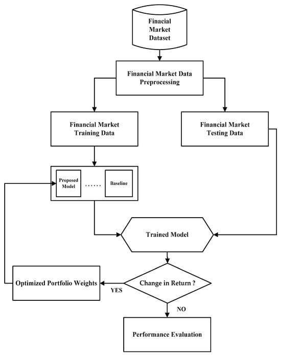
Figure 1.
The flow chart of the proposed scheme.
Once the features were prepared, a target variable was defined, often as a classification label indicating portfolio movement based on predefined return thresholds. The labelling was used to compare logarithmic return rates, using 0 and 1 to distinguish between negative and positive returns [57,58]. The missing values were addressed by using mean imputation. Subsequently, we used the z-score to identify outliers. Seventy percent (70%) of the financial market data was allocated for training, and the remaining thirty percent (30%) was used for testing [59,60]. The logistic regression model was trained on the historical (in-sample) data, where it learned the relationship between the features and the class labels using the logistic function.
Historical financial market data were used as inputs to the proposed scheme. These inputs included open, low, high, and close prices, as well as trading volume. More importantly, return and market volatility were derived from price data and employed as predictive features for market movement classification. Logistic regression, along with baseline models, was used to track market trends and estimate corresponding probabilities. These predictions were subsequently utilized to adjust the model’s weight dynamically based on the predicted probabilities. The portfolio optimization problem was addressed using the Lagrangian method, with the resulting weights applied to anticipate future market conditions. The logistic regression model’s tuning parameters were selected through L1 regularization guided by cross-validation, enhancing generalization. We used L1 regularization to prevent overfitting, especially in high-dimensional settings. The hyperparameter tuning was accomplished through the regularization strength for L1 penalties.
The logistic regression equation models the probability of an outcome Y ∈ [0, 1] as a function of predictor variables X. In the presence of uncertainty, an uncertainty term was incorporated into the model. We derived the differential equation for logistic regression with an added uncertainty term. Subsequently, the logistic regression model predicted a binary outcome (gain or loss) based on historical data using the key equations explained below. The logistic regression equation that models the probability P(Y = 1∣X) is as follows:
where
Y is the binary target (e.g., positive or negative stock return);
X1, X2, …, Xn are predictor variables (e.g., stock indicators);
The expression can be represented by
β0 is the intercept, and β1, β2, …, βn are the coefficients.
The term ϵ has been added to account for the uncertainty arising from the dynamics of the market environment. To express it in the form of a differential equation, we considered the rate of change of P(Y = 1∣X) with respect to z. The sigmoid function satisfies
With the uncertainty, Equation (23) will eventually become
If we substitute P(Y = 1∣X) with P, Equation (24) becomes
We introduced ϵ as a noise or error term (Gaussian or random) in both Equations (26) and (27) to account for rapid fluctuations caused by uncertainty over time, thereby mimicking real-world conditions. In our study, we assumed that uncertainty evolves as market prices change, and we modeled this behavior as a stochastic process. The term ϵ captures the random noise or uncertainty present in the input signal z, which is a common approach in stochastic or probabilistic models where inputs are not perfectly deterministic. Ultimately, there is the need to integrate the explicit uncertainty dynamics. This will result in
where
This eventually forms a differential equation that captures both the logistic regression dynamics [61] and the impact of time-varying uncertainty. The dynamic of the data input has a significant impact on the output [62].
Logistic regression estimates the log-odds of the target variable. This ensures that predictions remain within the range of (0,1) for probabilities. The log-odd can be calculated using Equation (28), as shown below:
The decision rule is primarily based on Equation (4); it can alternatively be written as follows:
During the training process, logistic regression employed maximum likelihood estimation (MLE) to determine the optimal parameters (). This approach maximized the probability of observing the given dataset. More importantly, the loss function (log loss) can be minimized using logistic regression to optimize the coefficients. Hence, the log loss can be computed as follows:
where is the actual outcome and is the predicted probability. The equations above played an integral role in predicting the outcomes based on historical data features. Hence, this eventually makes logistic regression a suitable technique for predicting markets and portfolios where probabilities are needed.
We used Lasso (L1) regularization in the logistic regression log-loss function by adding the term to Equation (30), where ζ is the regularization parameter that controls the penalty strength. The model weights are denoted by w, and d represents the number of features. This approach enhances model generalization by penalizing the absolute values of the coefficients, often resulting in sparse models with some coefficients reduced to zero. Consequently, it inherently performs feature selection by eliminating irrelevant features. Additionally, L1 regularization helps prevent overfitting, particularly in high-dimensional datasets.
Overfitting often occurs when the fitted model includes many feature variables with relatively large coefficient magnitudes. Incorporating regularization into logistic regression is essential for preventing overfitting. This is achieved by penalizing large coefficients, which helps ensure that the model remains simple and generalizable. More importantly, regularization mitigates the effects of multicollinearity by discouraging reliance on highly correlated predictors. The application of L1 regularization further enhances model performance by performing feature selection, assigning zero coefficients to less important predictors. Choosing the L1 regularization parameter (ζ) in logistic regression for financial market classification is a critical step, as it directly influences model sparsity, generalization capability, and the identification of meaningful predictors within noisy financial data. When ζ = 0, no regularization is applied, and the standard MLE solution is used. When ζ approaches ∞, all weights shrink toward zero, effectively nullifying the model. For values between 0 and ∞, a sparse solution is obtained (where some coefficients are zero while others remain active). To determine the optimal value of ζ, we employed cross-validation with a grid search approach to minimize out-of-sample prediction error. In this study, we set the regularization parameter ζ to 0.01. Also, the multicollinearity diagnostics showed no evidence of coefficient-sign instability due to collinear predictors.
As returns fluctuate, the system recalculates and re-optimizes portfolio weights based on model predictions. These updated weights are reintegrated into the training loop, allowing the model to adapt and improve continuously. If no significant market shift is detected, the model transitions to performance evaluation, where key metrics are computed to assess its effectiveness. This adaptive process ensures the system not only learns from historical patterns but also responds dynamically to market changes. The trained PALR scheme can predict the probability of positive or negative returns. It is also worth mentioning that other machine-learning techniques, such as Support Vector Machine (SVM), Discriminant, Random Forest (RF), and Decision Tree (DT), have been used to compare and evaluate the proficiency of the proposed scheme.
Dynamic portfolio return classification adapts to shifting financial markets by continuously updating its models and input features based on recent market conditions (return and volatility). These features are time-sensitive variables that capture the changing behavior of market participants. Observing shifts in volatility and return trends supports real-time reclassification of portfolio returns. This responsiveness ensures that the classification remains accurate even during sudden market shifts.
Finally, the performance of the scheme was evaluated using metrics such as accuracy, precision, recall, F1-score, and area under the ROC curve (AUC), along with other additional financial performance tools. These measures helped assess both the predictive capability of the model and its practical effectiveness in guiding dynamic portfolio decisions.
5. Experimental Result and Discussion
To critically examine the performance of the PALR scheme for predicting the returns of the DJIA and HSI financial markets, we carried out an experiment using a system with the following specifications. The proposed scheme was developed and thoroughly tested on a 2.7 GHz processor with 8 GB RAM and a 64-bit operating system. Different test conditions and experimental scenarios were also considered to assess the performance capability of the proposed scheme. In Section 5.1, we discuss the metrics used to evaluate the proficiency of the proposed algorithm and interpret the results.
5.1. Performance Evaluation and Comparison
This section primarily focuses on performance evaluation and comparison with other techniques. Hence, it is very important to discuss the metrics used to measure the prediction of the approaches used in simulation experimentation. The performance metrics used in this study include mean square error (MSE), precision, accuracy, F-score, and recall. These metrics have been used as tools to measure and compare the proficiency of the scheme with other conventional approaches. Specifically, we used these metrics to evaluate the performance of the proposed approach, and their mathematical representations are given below.
where
Rt and are the actual and predicted returns, respectively, at time t;
TP represents the correctly predicted positive cases;
TN represents the correctly predicted negative cases;
FP represents the incorrectly predicted positive cases;
FN represents the incorrectly predicted negative cases.
Statistically, the performance of the proposed scheme was analyzed and compared to RF, DT, Discriminant, and SVM. The performance metrics were used in comparing the scheme’s proficiency. Table 1 presents the results of model evaluations for predicting and classifying returns for the two financial indices, the DJIA and the HSI. Each model (RF, DT, Discriminant, SVM, and PALR) was assessed based on the following performance metrics: MSE, precision, accuracy, recall, and F-score. The computed values for each performance metric are presented in Table 1 below.

Table 1.
Performance metrics comparison.
5.1.1. Performance Evaluation Using the DJIA Dataset
First, we considered the MSE, precision, accuracy, recall, and F-score for each scheme based on the DJIA dataset, as shown in Table 1. The proposed PALR scheme exhibits a relatively low MSE of 0.0006 when compared to other schemes; this can be attributed to the simplicity and effectiveness of the PALR scheme in dealing with the probability-related outcomes. This clearly demonstrates that logistic regression achieved much better precision and accuracy, as the difference between the actual and predicted values is negligible. Nonetheless, it is evident that the DT scheme exhibits a lower MSE compared to RF, SVM, and the Discriminant scheme. Both SVM and Discriminant schemes achieved lower MSE compared to RF.
Based on the results obtained using the DJIA dataset, the highest classification accuracy was achieved with PALR (99.88%), followed by SVM (98.23%), Discriminant (97.91%), RF (96.10%), and DT (94.31%), respectively. Also, it should be noted that the least accuracy was achieved by DT amongst all the schemes.
Similarly, the performance of all the schemes was evaluated based on precision. As can be noticed from Table 1, PALR achieved the best precision performance of 99.97%. It is followed by SVM, with a precision of 98.36%. Then, Discriminant (96.82%), RF (94.66%), and DT (92.10%), respectively. DT had the lowest precision among the schemes.
Additionally, the recall of the schemes was evaluated using the DJIA dataset, measuring the true positive rate of each scheme. The highest recall was achieved using PALR (99.9%), followed by Discriminant (99.75%), DT (98.81%), SVM (98.32%), and RF (98.08%), respectively.
Furthermore, the highest F-score was achieved by PALR at 99.94%, followed by SVM with 98.33%. Similarly, Discriminant, RF, and DT achieved 98.26%, 96.33%, and 95.34%, respectively. Notably, it is worth mentioning that DT achieved the lowest F-score among all the classifiers.
5.1.2. Performance Evaluation Using the HSI Dataset
As shown in Table 1, the proposed PALR scheme outperformed all the compared schemes in evaluating performance using the HSI dataset. PALR once again outperformed all other classifiers, achieving an MSE of 0.0011 and consistent metrics of 99.89% across precision, accuracy, recall, and F-score. Discriminant delivered a strong F-score (97.94%) and recall (99.38%), making it competitive. DT achieved perfect precision (100%) but fell behind in accuracy (91.15%), recall (81.70%), and F-score (89.93%), indicating overfitting or imbalance in the predictions. RF and SVM underperformed on the HSI dataset compared to PALR, showing significantly higher MSE (0.1770 for RF and 0.1497 for SVM) and lower precision and F-score.
In summary, the results presented in Table 1 show that PALR consistently outperformed other algorithms in terms of MSE, accuracy, precision, recall, and F-score across both datasets (DJIA and HSI) used to evaluate the performance of the schemes. Hence, it demonstrates superior robustness and precision in the proposed dynamic portfolio return classification scheme. Discriminant ranks second on both datasets, particularly excelling in recall and F-score. SVM showed good overall performance on DJIA but struggled on HSI, potentially due to differences in the data distribution or feature dynamics. RF and DT were less effective, especially on the HSI dataset. Their performance metrics suggest difficulty in handling data complexity or noise. These results highlight PALR’s strength in capturing return dynamics, making it an optimal choice for portfolio classification tasks in financial markets.
5.2. Comparisons of Classifiers Using the Diebold–Mariano Test
In addition, the performance of the schemes was further evaluated using the Diebold–Mariano (DM) test on the two datasets. The DM test is a statistical method primarily designed to compare the accuracy of two competing classifiers. It assesses whether the difference in forecast accuracy between the classifiers is statistically significant. This test is particularly valuable in classifier selection, especially when the cost of inaccurate forecasts is high, such as in financial markets.
where
- d represents the mean of the loss differentials;
- represents the standard deviation of the loss differential;
- T is the sample size.
In addition, it is essential to highlight that the hypothesis was tested using a significance threshold. The threshold level was set at 0.05 (5%). The hypotheses for the DM test employed in this study are as follows:
- Null Hypothesis:The null hypothesis (Ho) of the test is that both classifiers have the same accuracy (i.e., no difference in performance). A rejection of the null hypothesis suggests that one classifier is significantly better than the other.
- Alternative Hypothesis:The alternative hypothesis (Hα) is that the forecast errors are significantly different, implying that one classifier outperforms the other.
We carried out a DM test to further assess and evaluate the effectiveness of the proposed PALR scheme using the DJIA and HSI datasets. The results are presented in Table 2 and Table 3, respectively.
Table 2.
Diebold–Mariano test comparison (DJIA).
Table 3.
Diebold–Mariano test comparison (HSI).
Table 2 presents the results of the DM test conducted using the DJIA dataset. Based on the information in Table 2, Classifier 1 and Classifier 2 represent the pairs of classifiers being compared. The DM statistic column can have either a negative or a positive value. A negative value indicates that Classifier 1 has smaller forecast errors and better accuracy than Classifier 2. Conversely, a positive value means that Classifier 2 has smaller forecast errors and better accuracy than Classifier 1. The p-value determines whether the difference in forecasting accuracy is statistically significant. If p < 0.05, the difference is considered statistically significant; if p ≥ 0.05, it is not. Lastly, the Significance Difference column indicates whether the classifiers differ significantly in accuracy (Yes) or not (No).
The DM test statistics show that PALR significantly outperformed all the other classifiers in terms of accuracy. PALR vs. RF: DM = −16.091, p = 0.0000 → PALR was more accurate than RF (since the DM value is negative and p < 0.05). PALR vs. SVM: DM = −11.0869, p = 0.0000 → PALR was more accurate than SVM. PALR vs. Discriminant: DM = −12.0373, p = 0.0000 → PALR was more accurate than the Discriminant classifier. PALR vs. DT: DM = −20.8801, p = 0.0000 → PALR was more accurate than DT.
Statistically, PALR is the best classifier, and it is better than all other classifiers. Both SVM and Discriminant exhibit very similar performances. Their results are superior to those of RF and DT. The performance of RF is better than DT but worse than SVM and Discriminant. Based on the DM test, DT is the worst-performing classifier amongst all the classifiers compared using the DJIA dataset. Ultimately, this clearly supports the results presented in Table 1.
As shown in Table 3, the DM test statistical results are derived from the HSI dataset. Statistically, PALR was significantly more accurate than RF, SVM, Discriminant, and DT (since its DM value is negative when compared to the DM value of RF, SVM, Discriminant, and DT). In addition, the Discriminant method was better than RF, SVM, and DT. Based on the DM test, it is evident that DT outperforms RF and SVM. However, its accuracy is lower than that of PALR and Discriminant. RF is significantly less accurate when compared to all other classifiers. Statistically, the DM test supports the results shown in Table 1, demonstrating that PALR significantly outperforms all other classifiers in terms of accuracy.
5.3. Comparisons of Classifiers Using Thiel’s U-Statistic
In addition, we used Thiel’s U-statistics to evaluate forecast accuracy by comparing predicted values to actual values. It helps determine how well a forecasting model performs relative to a naïve model (typically a random walk or simple mean model). More importantly, it accounts for both the magnitude of errors and the direction of changes. This makes it particularly useful in economic and financial forecasting. The formula for Thiel’s U-statistic test is as follows:
where
- Pt is the predicted value at time t;
- At is the actual value at time t;
- T is the number of observations.
The value of U ranges from 0 to 1. For U = 0, the predicted values perfectly match the actual values. In a situation where U < 1, it shows that the model is better than a naïve forecast. If U > 1, it indicates that the model performs worse than a naïve forecast. Each of the classifiers was tested using the DJIA and HSI datasets to determine the U-statistic value. The U-statistic values obtained are presented in Table 4, shown below.
Table 4.
U-Statistic test comparison.
As shown in Table 4, PALR achieved U-stat values of 0.0011 and 0.0021 when evaluating the classifier using the DJIA and HSI datasets, respectively. PALR consistently showed the smallest U-statistics for both datasets, suggesting it has the most accurate forecasts compared to the others. RF performed relatively poorly on the HSI dataset, indicating larger forecast errors compared to other classifiers. SVM performed better than RF but still shows significant forecast errors, especially for the HSI dataset. The Discriminant classifier achieved moderate performance, better than RF and SVM, but worse than PALR. DT showed the weakest performance for the DJIA dataset and performed moderately for the HSI dataset. DT tended to perform the worst, particularly for the DJIA dataset. RF shows surprisingly poor results for the HSI dataset. The classifiers’ performance differs between DJIA and HSI, with larger U-statistics observed for HSI. This indicates that classifying the HSI market could be more challenging in general. PALR is the most accurate classifier for both the DJIA and HSI datasets, as indicated by the smallest U-statistic values. This aligns with the PALR performance presented in Table 1, Table 2, and Table 3, respectively.
5.4. AUC Curves Comparison
Additionally, the performance of the proposed scheme was compared to DT, RF, SVM, and Discriminant in terms of area under the curve (AUC). It is an essential performance measurement tool used to distinguish between classes across different thresholds. Specifically, the AUC is calculated as the area under the receiver operating characteristic (ROC) curve. The plot of the TP rate against the FP rate for all the schemes, based on the two datasets used, is shown graphically in Figure 2 and Figure 3.
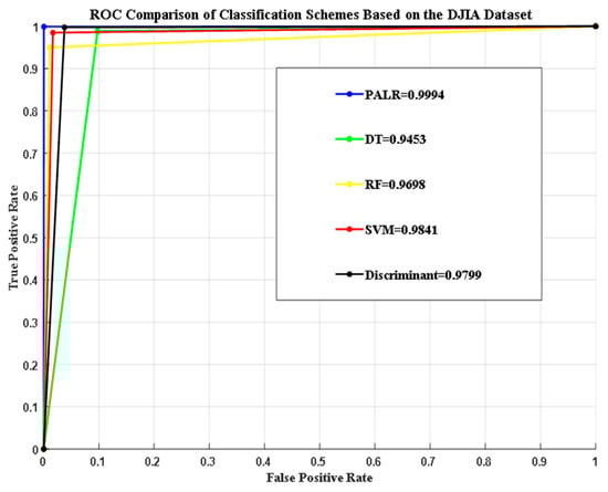
Figure 2.
AUC curves comparisons based on the DJIA dataset.
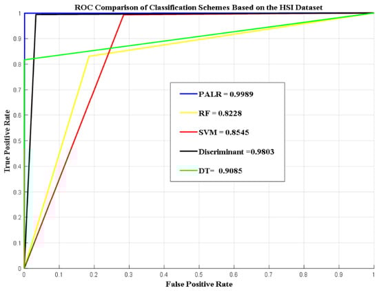
Figure 3.
AUC curves comparisons based on the HSI dataset.
As shown in Figure 2, the proposed scheme based on PALR was able to achieve an AUC of 99.94%. The proposed scheme outperformed all other algorithms based on the AUC curve, as shown above. This demonstrates that the classifier can distinguish between the classes with minimal errors across all thresholds. The proposed scheme demonstrated exceptionally high precision and recall, with no overlap between the positive and negative classes. While the AUC achieved by the RF scheme was around 96.9%, indicating good performance, it had slightly more misclassification compared to the PALR scheme. SVM achieved an AUC of 98.4%, demonstrating high accuracy. However, minor inconsistencies were observed across the threshold. The Discriminant attained an AUC of 97.9%, which is lower than that of the PALR and SVM schemes. DT had the lowest AUC of 94.53% compared to PALR, RF, SVM, and the Discriminant scheme. In summary, PALR achieved the highest AUC, which is crucial for critical applications such as financial forecasting and medical diagnostics.
Figure 3 shows the AUC curves comparison of schemes based on the HSI dataset. Based on the graphs presented in Figure 3, PALR stands out as the best classifier. Its AUC value of 0.9989, nearly reaching 1, indicates a highly reliable classification capability. PALR captured the underlying patterns in the HSI dataset exceptionally well, leveraging its dynamic and price-sensitive modeling. The high AUC aligns with its uniformly high precision, recall, and F-score. While Discriminant (0.9803) was competitive with PALR, offering excellent discrimination, it is slightly less robust than PALR. Thus, Discriminant analysis effectively handled the linear separability of the dataset, achieving strong class distinction. Its high AUC reflects consistent performance across a range of thresholds. Both SVM (0.8545) and RF (0.8228) provided acceptable discrimination. However, they lagged behind PALR and Discriminant analysis, highlighting the challenges in fully capturing the complexities of the HSI dataset. DT had an AUC of 0.9085, which strikes a balance between interpretability and discrimination but is less effective than PALR and Discriminant analysis in terms of generalization. These AUC scores affirm PALR’s superiority for dynamic portfolio return classification when tested using the HSI dataset.
5.5. Precision-Recall Curves Comparison
Furthermore, the precision–recall (PR) curves for all the schemes based on the two datasets (DJIA and HSI) were analyzed and plotted. The PR curve is a visualization tool used to evaluate the performance of classification models, particularly for imbalanced datasets where one class significantly outnumbers the other. The PR curve provides insight into the trade-off between precision (positive predictive value) and recall (sensitivity) across different decision thresholds.
Figure 4 presents a comparison of the PR curves for the schemes based on the DJIA dataset. The proposed PALR scheme outperformed all other classifiers, as its PR curve remains close to the top-right corner, clearly indicating high precision and recall. Ultimately, this can be proven from the performance metric results shown in Table 1. It clearly demonstrates that PALR achieved high precision and recall of 99.97% and 99.9%, respectively. The area under the PR curve is closer to (1,1) in the PR space, indicating near-perfect precision and recall. The PALR’s high precision indicates that most of the predicted positives are actual positives, thereby minimizing false positives. Its high recall shows the classifier effectively identifies most actual positive cases, minimizing false negatives. Discriminant has a better PR curve compared to DT, SVM, and RF, while RF has the least PR curve, which truly coincides with the results shown in Table 1. As shown in Figure 4, increasing recall typically decreases precision, and vice versa. The PR curve helps determine an optimal threshold by analyzing the trade-off between precision and recall, and it provides an effective way to compare the classifiers. The PR curves for the classifiers based on the HSI dataset are presented graphically in Figure 5.
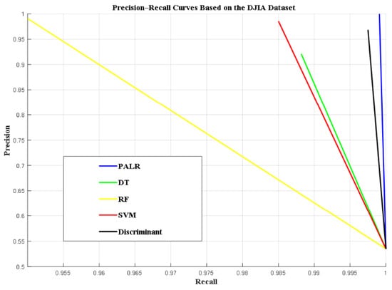
Figure 4.
Precision–recall curves comparison based on the DJIA dataset.
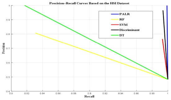
Figure 5.
Precision–recall curves comparison based on the HSI dataset.
Figure 5 presents the graphical representation of PR curves for all the schemes based on the HSI dataset. The proposed PALR achieved the best balance between precision and recall, which ultimately makes it the most reliable classifier for the HSI dataset. It effectively identified true positives while minimizing FP and FN. Also, the Discriminant performed exceptionally well, with high recall indicating it captured nearly all relevant instances. However, its precision was lower than PALR, meaning it had a slightly higher rate of false positives. SVM also had excellent recall, retrieving nearly all relevant instances. However, its low precision suggests more false positives, reducing its reliability compared to PALR and Discriminant. Similarly, DT achieved perfect precision, indicating that all its predicted positives were true positives. However, its recall was relatively low, indicating it missed a significant number of relevant instances. Furthermore, RF was less effective compared to other classifiers. It had relatively balanced but unimpressive precision and recall, which might limit its usefulness for this classification task. In conclusion, the PR curve shows PALR at the top-right corner, followed by Discriminant, while DT excels on the precision axis. SVM is higher on the recall axis of the PR curve, but lower on precision. Lastly, RF possessed the lowest precision and recall on both PR curve axes. Thus, its balanced but unimpressive precision and recall may limit its usefulness for this classification task. PALR again outperforms all other classifiers in terms of the PR curve, as shown in Figure 5.
In addition, we compared the performance of PALR with other studies in the literature using accuracy as the evaluation metric. The results clearly demonstrate that the proposed PALR scheme outperforms existing approaches, achieving an accuracy of 99.88% when evaluated on the DJIA and HSI datasets. The comparison is shown in Table 5 below.
Table 5.
PALR accuracy comparison with other studies.
5.6. Stress Testing Under Financial Crisis Period Conditions
To further assess the robustness of the proposed model in extreme market conditions, we conducted a stress-testing analysis by isolating a well-known financial crisis: 2008’s Global Financial Crisis. During this period, market volatility and systemic risk surged significantly, making it ideal for evaluating model stability and adaptability.
To perform a machine-learning stress test for stock performance during the 2008 Global Financial Crisis, we considered the two datasets (DJIA and HSI) used in our work. We extracted the logs of the financial data during the crisis period (September 2008–March 2009) from both datasets. The non-crisis period data was used to train PALR separately based on stock prices, financial indicators, macroeconomic variables, and relevant market indices. This allowed PALR to learn typical market behavior. After training, the model was tested on data from the crisis period without retraining to evaluate how well it could generalize and make predictions under extreme conditions. Subsequently, the key performance metrics like accuracy, standard deviation (SD), and MSE revealed how stress-resistant the model is, especially in identifying abnormal behaviors. This stress-testing framework helps assess both the resilience of PALR and its ability to support investment decisions during periods of systemic financial stress. The results obtained from the stress test are presented in Table 6.
Table 6.
Stress testing on PALR’s classification capability.
Table 6 presents a comparative evaluation of classification performance using the DJIA and HSI datasets across two market conditions: non-crisis and crisis periods. Three performance metrics were used: classification accuracy, MSE, and standard deviation (SD). During the crisis period, both DJIA and HSI models achieved perfect classification accuracy (1.0) with zero error (MSE = 0) and no variation in prediction errors (SD = 0), indicating good predictive performance under extreme market conditions. In the non-crisis period, both indices still performed exceptionally well, with classification accuracies of 0.9995 (DJIA) and 0.9990 (HSI). MSE values were very low (0.000495 for DJIA, 0.000539 for HSI), and SD was minimal (0.031 for DJIA, 0.027 for HSI).
Overall, the results suggest that the predictive model maintained high accuracy and robustness across different market regimes, with slightly better performance for DJIA in stable conditions.
5.7. PALR Explainability and Interpretability
This section primarily focuses on the explainability and interpretability of the proposed scheme. It has been included to explain how financial variables contribute to portfolio classification decisions. This allows investors and analysts to understand which features influence portfolio positions, assess risk exposure, and maintain trust in the system’s outputs. Additionally, interpretability supports regulatory compliance and enhances the robustness of the trading strategy by exposing potential biases or misalignments in the data-driven decision process. Hence, the explainability and interpretability analysis of PALR is achieved using the SHapley Additive exPlanations (SHAP), which shows the impact of the features on the model output. SHAP is a powerful framework used to explain the output of machine-learning models. Its significance lies in its ability to quantify the contribution of each feature to a model’s prediction using a solid game-theory foundation. We selected SHAP over LIME primarily because it provides consistent and theoretically grounded feature attributions based on Shapley values. SHAP offers global interpretability while maintaining local accuracy, making it particularly effective for understanding model behavior across varying market conditions [67]. Both the DJIA and HSI have been used in the PALR model’s transparency, feature importance, trust, and accountability analysis. SHAP helps bridge the gap between predictive accuracy and interpretability.
Figure 6 presents the SHAP summary plots, illustrating the overall impact of each feature on the PALR model’s output across the entire DJIA and HSI datasets. The plots convey both the importance of each feature and the direction of its influence. As shown in Figure 6a, return is the most influential feature, with a wide spread of SHAP values ranging from highly negative to highly positive. The high return values (red) tend to increase the model output (positive SHAP values), while the low return values (blue) tend to decrease the output. This strong influence of return on predictions is indicated by the long horizontal spread along the x-axis. This means that both very high and very low return values can significantly influence the model’s prediction in opposite directions. Volatility is the next most impactful feature, typically contributing negatively to the prediction when its values are high (as indicated by red dots on the left), which suggests the model may associate high volatility with unfavorable outcomes. Open, close, high, and low exhibit relatively low variation in their SHAP values, indicating a limited and consistent influence on the model’s predictions. While they do contribute to the output, their impact is less variable. Among the listed features, volume has the least influence, as reflected by its very narrow SHAP value range. The compact clustering of the SHAP values around zero implies the influence is relatively minor across most samples. As shown in Figure 6b, return is the influential feature, and its SHAP values range from highly negative to positive when tested on the HSI dataset. Open, volatility, and close also significantly affect the output, while high and low features have less minimal impact on the model prediction. Volume has the least minimal influence on the model prediction amongst all other features. The plot reveals not only which features matter most but also how their values push predictions higher or lower.
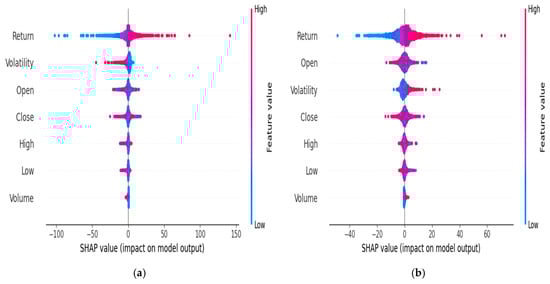
Figure 6.
SHAP value impact on PALR output based on the (a) DJIA and (b) HSI datasets.
Furthermore, we used SHAP bar plots to provide a clear, quantitative explanation of how each feature contributes to PALR’s prediction. Consequently, this enhances interpretability, trust, and decision-making. SHAP bar plots show not just how important a feature is, but also whether it increases or decreases the prediction. We considered both the DJIA and HSI datasets, and their respective SHAP bar plots are presented in Figure 7, shown below.
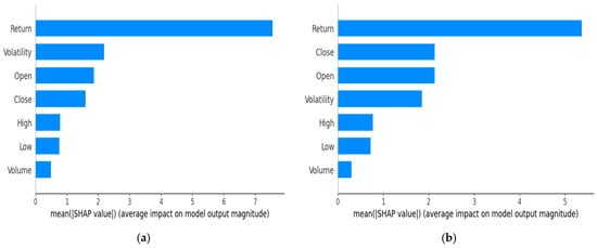
Figure 7.
SHAP bar plots based on the (a) DJIA and (b) HSI datasets.
Figure 7 shows the SHAP bar plots, which summarize the average impact of each feature on the model’s predictions based on the two datasets (DJIA and HSI). They are ranked using the mean absolute SHAP value. Although the order of the feature contributions differs, the topmost impactful features are the same. It can be noted that the return contribution using DJIA is high when compared to HSI. Figure 7a shows that return is the most important feature, having the largest overall influence on the model’s output when evaluated using the DJIA dataset. Then, it is followed by volatility, which also contributes significantly. Open and close have progressively smaller effects, indicating they play a less critical role in the portfolio classification decision-making. High, low, and volume features play less significant roles when compared to other features. As illustrated in Figure 7b, return has the highest average impact, indicating it is the most influential factor in the PALR’s decision-making process when using the HSI dataset. Close, open, and volatility follow as the next most important features, each contributing meaningfully but to a lesser extent compared to return. Features such as high, low, and especially volume have relatively low average SHAP values, suggesting they play a minor role in influencing the model’s output. These plots provide a clear summary of feature importance by quantifying the magnitude of their effect across all predictions. It is noteworthy that in both cases, the features with the highest and lowest contribution are the same, based on the SHAP feature contribution presented in Figure 7.
To further interpret the PALR coefficients and their exponentiated values, we compared the feature coefficients derived from each dataset. Given the application of normalization as described in Section 4, the absolute magnitudes of the logistic regression coefficients and their corresponding odds ratios should be interpreted only in relative terms; that is, as a comparison of predictor importance, rather than as direct effect sizes. The comparison is presented in Table 7 below.
Table 7.
PALR coefficients and exponentiated coefficients comparison.
Table 7 presents the coefficients (B) and exponentiated coefficients (Exp(B)) obtained from PALR’s two different datasets: the DJIA and HSI. These values indicate how different features affect the probability of the PALR outcome. For both indices, return has a large positive coefficient and a very high Exp(B), indicating it strongly increases the odds of the predicted event. Volatility negatively affects DJIA outcomes (B = −4.1252) but positively influences HSI, indicating that volatility plays opposing roles in the two markets. Other features like open, close, high, low, and volume show smaller effects, with odds ratios close to 1, implying relatively minor influence. The contrasting signs and magnitudes highlight differences in how these features impact predictions in each dataset. It is noteworthy that volume and price are fundamental indicators in financial markets, closely tied to investor sentiment and overall market dynamics. Price captures the perceived value of an asset, responding to the cumulative effect of market information, while volume reflects the degree of participation or confidence driving those price movements. Although each variable may seem marginal in isolation, their combined behavior often reveals critical patterns such as momentum, trend strength, or potential reversals, key factors in gain/loss classification tasks. For example, a price increase accompanied by high trading volume typically signals stronger bullish sentiment than the same increase with low volume. Therefore, even slight fluctuations in these indicators can influence classification outcomes by offering valuable context on the persistence or volatility of market trends.
We also utilized the SHAP waterfall plot to visualize how each feature contributes to an individual prediction made by the machine-learning model. This plot decomposes the output of the PALR model by illustrating the cumulative effect of each feature’s SHAP value, starting from the baseline. The SHAP waterfall plots for both the DJIA and HSI are presented in Figure 8 below.
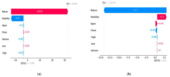
Figure 8.
SHAP waterfall plots based on the (a) DJIA and (b) HSI datasets.
Figure 8 presents the SHAP waterfall plot for the DJIA and HSI datasets. Figure 8a illustrates how individual features contribute to a single prediction made by a model. The base value on the far left, E[f(x)] = −3.295, represents the average prediction across the dataset. Each feature then pushes the prediction up or down, with the final output being f(x) = 32.605 on the far right. The largest positive contributor is the return, which increases the prediction significantly by +45.87, shown in red. In contrast, volatility has the largest negative effect, decreasing the prediction by −9.91, shown in blue. The close and low features contribute modestly and positively to the prediction. In contrast, the remaining features—open, volume, and high—exert relatively minor negative influences, with SHAP values of −0.2, −0.08, and −0.03, respectively. The visualization provides a step-by-step breakdown of the prediction process, illustrating how each feature’s individual contribution aggregates to form the model’s final output for this specific instance. Statistically, the return for the DJIA during the examined period was positive, aligning with the results presented in Figure 8a. Figure 8b illustrates the contribution of each feature to a single prediction made by the PALR model when evaluated on the HSI dataset. The baseline value, shown on the far right as E[f(x)] = 0.52, represents the average model output across the dataset. The model’s prediction for this specific instance was f(x) = −14.027, which results from adding the SHAP values of individual features to the baseline. The return had the largest negative impact, reducing the prediction by 17.1, while volatility increased it by 2.5, the most significant positive contribution. The open, low, and volume features had a slight positive impact on the prediction, whereas the close and high features contributed minimally, with a slight negative influence. This plot effectively traces how the model arrived at the final output by summing up the individual effects of each feature. The results obtained show that the two financial markets examined are entirely different in terms of the return achieved by each: the DJIA recorded a positive return, while the HSI exhibited a negative return during the period examined.
To summarize the findings of the evaluations and analysis conducted on all the classifiers and datasets used in this study, the PALR classifier consistently demonstrated superior performance compared to other classification schemes (RF, DT, SVM, and Discriminant) for both the DJIA and HSI datasets due to its capability and ability to handle dynamic financial environments. It had high precision and recall, exceptional accuracy, was robust across all datasets, and had better generalization and superior AUC and PR curves. PALR uniquely integrates price-aware features, enhancing its performance. Combined with logistic regression adaptability, this allows PALR to outperform traditional classifiers in precision, recall, accuracy, and robustness. Its ability to adapt to market dynamics and generalize well across different datasets makes it a highly reliable classification scheme. This adaptability solidifies it as the most effective approach for dynamic portfolio return prediction in uncertain financial market environments.
6. Conclusions
In this paper, we proposed a PALR scheme that adapts to changing market conditions and improves prediction accuracy compared to conventional methods. More importantly, the proposed dynamic portfolio-based return prediction algorithm offers a robust solution for return prediction in uncertain financial markets. It dynamically adjusts portfolio weights in response to changing market conditions, effectively addressing the challenges posed by market volatility. This algorithm enhances predictive accuracy and reduces risk exposure. The integration of machine learning enables continuous refinement of the PALR model, helping investors make more informed decisions. Ultimately, this demonstrated the capability of the proposed model in terms of accuracy, precision, and robustness. Also, it is worth mentioning that the scheme adapts to various financial market conditions, thereby enhancing the practical applicability of the proposed scheme in real-time. The experimental results showed that the PALR scheme outperformed RF, SVM, DT, and Discriminant in terms of accuracy, precision, recall, MSE, F-score, AUC, and PR curve.
This study presents a method for classifying dynamic portfolio returns, applicable to portfolio optimization and management. Both theoretically and practically, the proposed approach has shown promising results with negligible classification errors when tested on the DJIA and HSI datasets. More importantly, the proposed PALR scheme will ultimately support investors, asset and portfolio managers, and financial institutions in developing investment strategies and making effective investment decisions. Consequently, this will significantly reduce the time and resources required by investors and managers to make informed decisions.
To address the issue of potential overfitting, which is critical in financial modeling, both train–test splitting with temporal separation and L1 (Lasso) regularization were employed. The temporal split was used to simulate out-of-sample prediction, ensuring that future data did not leak into the training process. Additionally, L1 regularization was incorporated into the logistic regression framework to penalize model complexity and further mitigate overfitting.
The integration of PALR into real-time trading systems enables adaptive portfolio decision-making by dynamically responding to market fluctuations using price-sensitive features. This real-time capability enhances execution timing and risk-adjusted returns. From a regulatory perspective, PALR can support transparent and explainable AI-driven trading decisions, aligning with growing compliance demands for model interpretability and auditability. It can also help regulators by spotting unusual trading patterns or market problems. This supports better monitoring and policy decisions. Moreover, PALR is grounded in economic theory by incorporating rational market signals and aligns with observed investor behavior, such as trend-following and risk aversion, thereby bridging data-driven models with behavioral finance insights.
To implement PALR in an operational setting, the model can be embedded within an automated trading system consisting of four core modules: (1) real-time data ingestion, where live financial data streams (prices, volume, news sentiment) are collected via APIs; (2) a feature engineering layer, which computes rolling volatility, momentum indicators, and adjusted price signals; (3) an inference engine, where the trained PALR model classifies current portfolio positions based on real-time features; and (4) execution and feedback, where trades are placed via brokerage APIs and outcomes are logged for continual model refinement. The model’s probabilistic outputs can also be integrated into risk-weighted decision thresholds, allowing for flexibility depending on market volatility. This end-to-end setup ensures PALR can adapt dynamically and provide timely, data-driven decisions within live financial systems.
While the PALR model improves responsiveness to market dynamics, it also presents certain limitations. Its performance is highly dependent on preprocessing decisions—such as normalization techniques, window size, and cross-validation—which can greatly affect both predictive accuracy and model stability. Inconsistent or suboptimal preprocessing may introduce bias or generate misleading trading signals. Additionally, applying PALR in less liquid or emerging markets poses challenges. These markets often display irregular price movements, lower trading volumes, and heightened volatility, all of which can undermine the model’s effectiveness and may necessitate further calibration or alternative modeling strategies.
PALR is built on logistic regression, which is inherently interpretable. Each feature’s impact on decision-making (e.g., volatility, return, price movement) can be quantified. This allows for clear explanations to stakeholders, auditors, and clients. This eventually fulfils the MiFID II requirements for algorithmic transparency and investor protection. In addition, the model integrates real-time price signals, which can be updated periodically, allowing for responsive risk management. The ability to dynamically classify portfolios based on volatility and return helps in the early detection of excessive risk exposure. This aligns with risk governance standards under MiFID II and Basel III. Since PALR is statistically grounded, it will enable full audit trails needed by regulators. In advisory settings, PALR can be adapted to consider investor-specific constraints (e.g., risk tolerance, investment horizon), ensuring portfolio recommendations remain suitable and compliant with client profiling requirements.
It is evident that there is a pressing need to explore the capabilities of PALR as a tool for classifying smaller, emerging, or less liquid markets. These markets often exhibit unique structural characteristics, such as heightened volatility, lower liquidity, and irregular trading patterns, which require careful study. While our current study primarily focuses on large, liquid markets to establish the core performance of PALR, the model is inherently designed with flexibility. Its dynamic adjustment mechanism is driven by price movements and returns. It can be calibrated for alternative market environments through tailored feature selection, threshold tuning, and regularization adjustments. Therefore, it is crucial to empirically validate the performance of PALR in emerging or less liquid markets in our future research. More importantly, future research will explore the effects of alternative data preparation strategies, return definitions, and prediction horizons.
In our future research, we will incorporate more diverse data sources, including macroeconomic indicators, sentiment analysis, and technical indicators. Hence, these will provide a more comprehensive view of the market dynamics, enabling investors and traders to make informed decisions with greater confidence. Essentially, this will explore potential trading opportunities that adapt to the portfolio dynamics in a rapidly changing market environment. In future extensions, we also plan to explore online learning strategies or retraining at fixed intervals to enhance adaptability in real-time applications. Furthermore, to enhance the risk assessment of the dynamic portfolio, we will incorporate additional robust risk measures, such as value at risk (VaR), to better capture tail risk. Ultimately, this would provide a more comprehensive understanding of downside risk, especially under non-normal return distributions.
Author Contributions
Conceptualization, Y.S.B. and H.M.A.; Methodology, Y.S.B.; Software, Y.S.B.; Validation, Y.S.B.; Formal analysis, Y.S.B.; Investigation, Y.S.B.; Resources, H.M.A. and A.A.T.; Writing—review & editing, A.A.T.; Funding acquisition, Y.S.B. and H.M.A. All authors have read and agreed to the published version of the manuscript.
Funding
This work was supported by the Deanship of Scientific Research (DSR), King Abdulaziz University, Saudi Arabia [grant number D-64-830-1437].
Data Availability Statement
The data presented in this study are openly available in Yahoo finance website. [Yahoo finance] [https://finance.yahoo.com/].
Acknowledgments
The authors would like to thank all those who contributed to making this research successful. Also, we would like to thank the reviewers for their insightful and valuable comments. This work is supported by the Deanship of Scientific Research (DSR), King Abdulaziz University, Saudi Arabia. The authors are very grateful to the DSR for their technical and financial support throughout the period of the project.
Conflicts of Interest
The authors declare no conflicts of interest.
References
- Battauz, A.; De Donno, M.; Sbuelz, A. Reaching nirvana with a defaultable asset? Decis. Econ. Financ. 2017, 40, 31–52. [Google Scholar] [CrossRef]
- Hamdani, Z.; Dif, A.; Zairi, B.; Benziane, A.; Hamdani, M. Factors Affecting the Behavior of Financial Markets in the Light of Financial Risks. In Advances in Human Factors, Business Management and Leadership: Proceedings of the AHFE 2020 Virtual Conferences on Human Factors, Business Management and Society, and Human Factors in Management and Leadership, 16–20 July 2020, USA; Springer International Publishing: Cham, Switzerland, 2020; Volume 1209. [Google Scholar]
- Johannes, M.; Korteweg, A.; Polson, N. Sequential Learning, Predictability, and Optimal Portfolio Returns. J. Financ. 2014, 69, 611–644. [Google Scholar] [CrossRef]
- Lio, W.; Liu, B. Uncertain maximum likelihood estimation with application to uncertain regression analysis. Soft Comput. 2020, 24, 9351–9360. [Google Scholar] [CrossRef]
- Das, B.; Tripathy, B.C.; Debnath, P.; Bhattacharya, B. Characterization of statistical convergence of complex uncertain double sequence. Anal. Math. Phys. 2020, 10, 71. [Google Scholar] [CrossRef]
- Ding, J.; Zhang, Z. Statistical inference on uncertain nonparametric regression model. Fuzzy Optim. Decis. Mak. 2021, 20, 451–469. [Google Scholar] [CrossRef]
- Liu, Z.; Yang, Y. Least absolute deviations estimation for uncertain regression with imprecise observations. Fuzzy Optim. Decis. Mak. 2019, 19, 33–52. [Google Scholar] [CrossRef]
- Song, Y.; Fu, Z. Uncertain multivariable regression model. Soft Comput. 2018, 22, 5861–5866. [Google Scholar] [CrossRef]
- Yao, K.; Liu, B.D. Uncertain regression analysis: An approach for imprecise observations. Soft Comput. 2017, 22, 5579–5582. [Google Scholar] [CrossRef]
- Budhi, H.; Yeny, K.F.; Fajar, I. Quantifying Uncertainty of Insurance Claims Based on Expert Judgments. Mathematics 2025, 13, 245. [Google Scholar] [CrossRef]
- Tobek, O.; Hronec, M. Does it pay to follow anomalies research? Machine learning approach with international evidence. J. Financ. Mark. 2021, 56, 100588. [Google Scholar] [CrossRef]
- Pieter, M.V.; Dang, D.; Forsyth, A.P. The surprising robustness of dynamic Mean-Variance portfolio optimization to model misspecification errors. Eur. J. Oper. Res. 2021, 289, 774–792. [Google Scholar]
- Chang, H. Dynamic mean–variance portfolio selection with liability and stochastic interest rate. Econ. Model. 2015, 51, 172–182. [Google Scholar] [CrossRef]
- Gao, J.; Li, D.; Cui, X.; Wang, S. Time cardinality constrained mean–variance dynamic portfolio selection and market timing: A stochastic control approach. Automatica 2015, 54, 91–99. [Google Scholar] [CrossRef]
- Cheng, Z.; Xiaomin, G.; Jingshu, Z.; Zhiwei, C. Dynamic portfolio allocation for financial markets: A perspective of competitive-cum-compensatory strategy. J. Int. Financ. Mark. Inst. Money 2023, 84, 101737. [Google Scholar]
- Guo, S.; Yu, L.; Li, X.; Kar, S. Fuzzy multi-period portfolio selection with different investment horizons. Eur. J. Oper. Res. 2016, 254, 1026–1035. [Google Scholar] [CrossRef]
- Mansour, N.; Cherif, M.S.; Abdelfattah, W. Multi-objective imprecise programming for financial portfolio selection with fuzzy returns. Expert Syst. Appl. 2019, 138, 112810. [Google Scholar] [CrossRef]
- Gong, X.; Min, L.; Yu, C. Multi-period portfolio selection under the coherent fuzzy environment with dynamic risk-tolerance and expected-return levels. Appl. Soft Comput. 2022, 114, 108104. [Google Scholar] [CrossRef]
- Gupta, P.; Mehlawat, M.K.; Khan, A.Z. Multi-period portfolio optimization using coherent fuzzy numbers in a credibilistic environment. Expert Syst. Appl. 2021, 167, 114135. [Google Scholar] [CrossRef]
- Chen, W.; Zhang, H.; Mehlawat, M.K.; Jia, L. Mean-variance portfolio optimization using machine learning-based stock price prediction. Appl. Soft Comput. 2021, 100, 106943. [Google Scholar] [CrossRef]
- Li, B.; Zhang, R. A new mean-variance-entropy model for uncertain portfolio optimization with liquidity and diversification. Chaos Solitons Fractals 2021, 146, 110842. [Google Scholar] [CrossRef]
- Lee, S.I.; Yoo, S.J. Threshold-based portfolio: The role of the threshold and its applications. J. Supercomput. 2018, 76, 8040–8057. [Google Scholar] [CrossRef]
- Rezaei, H.; Faaljou, H.; Mansourfar, G. Stock price prediction using deep learning and frequency decomposition. Expert Syst. Appl. 2021, 169, 114332. [Google Scholar] [CrossRef]
- Ma, Y.; Han, R.; Wang, W. Portfolio optimization with return prediction using deep learning and machine learning. Expert Syst. Appl. 2021, 165, 113973. [Google Scholar] [CrossRef]
- Du, J. Mean–variance portfolio optimization with deep learning based-forecasts for cointegrated stocks. Expert Syst. Appl. 2022, 201, 117005. [Google Scholar] [CrossRef]
- Baek, Y.; Kim, H. ModAugNet: A new forecasting framework for stock market index value with an overfitting prevention LSTM module and a prediction LSTM module. Expert Syst. Appl. 2018, 113, 457–480. [Google Scholar] [CrossRef]
- Wang, J.; Wang, J. Forecasting stock market indexes using principle component analysis and stochastic time effective neural networks. Neurocomputing 2015, 156, 68–78. [Google Scholar] [CrossRef]
- Deng, Y.; Bao, F.; Kong, Z.; Ren, Z.; Dai, Q. Deep direct reinforcement learning for financial signal representation and trading. IEEE Trans. Neural Networks Learn. Syst. 2016, 28, 653–664. [Google Scholar] [CrossRef]
- Guo, Y.; Fu, X.; Shi, Y.; Liu, M. Robust log-optimal strategy with reinforcement learning. arXiv 2018, arXiv:1805.00205v1. [Google Scholar]
- Moallemi, C.C.; Saglam, M. Dynamic portfolio choice with linear rebalancing rules. J. Financ. Quant. Anal. 2017, 52, 1247–1278. [Google Scholar] [CrossRef]
- Zhang, J.; Jin, Z.; An, Y. Dynamic portfolio optimization with ambiguity aversion. J. Bank. Financ. 2017, 79, 95–109. [Google Scholar] [CrossRef]
- Mei, X.; Nogales, F.J. Portfolio selection with proportional transaction costs and predictability. J. Bank. Financ. 2018, 94, 131–151. [Google Scholar] [CrossRef]
- Collin-Dufresne, P.; Daniel, K.D.; Saglam, M. Liquidity regimes and optimal dynamic asset allocation. J. Financ. Econ. 2020, 136, 379–406. [Google Scholar] [CrossRef]
- Gârleanu, N.; Pedersen, L.H. Dynamic portfolio choice with frictions. J. Econ. Theory 2016, 165, 487–516. [Google Scholar] [CrossRef]
- Gârleanu, N.; Pedersen, L.H. Dynamic trading with predictable returns and transaction costs. J. Financ. 2013, 68, 2309–2340. [Google Scholar] [CrossRef]
- Bouchard, B.; Fukasawa, M.; Herdegen, M.; Muhle-Karbe, J. Equilibrium returns with transaction costs. Financ. Stoch. 2018, 22, 569–601. [Google Scholar] [CrossRef]
- Weiyi, Z.; Zhou, H.; Bao, X.; Cui, H. Outlet water temperature prediction of energy pile based on spatial-temporal feature extraction through cnn–lstm hybrid model. Energy 2023, 264, 126190. [Google Scholar]
- Wu, J.M.; Zhongcui, L.; Norbert, H.; Bay, V.; Jerry, C.L. A graph-based CNN-LSTM stock price prediction algorithm with leading indicators. Multimed. Syst. 2023, 29, 1751–1770. [Google Scholar] [CrossRef]
- Lu, W.; Jiazheng, L.; Jingyang, W.; Lele, O. A cnn-bilstm-am method for stock price prediction. Neural Comput. Appl. 2021, 33, 4741–4753. [Google Scholar] [CrossRef]
- Mienye, I.D.; Yanxia, S. Performance analysis of cost-sensitive learning methods with application to imbalanced medical data. Inform. Med. Unlocked 2021, 25, 100690. [Google Scholar] [CrossRef]
- Chong, E.; Chulwoo, H.; Frank, C.P. Deep learning networks for stock market analysis and prediction: Methodology, data representations, and case studies. Expert Syst. Appl. 2017, 83, 187–205. [Google Scholar] [CrossRef]
- Widiputra, H.; Harya, A.M.; Elliana, G. Multivariate CNN-LSTM model for multiple parallel financial time-series prediction. Complexity 2021, 2021, 9903518. [Google Scholar] [CrossRef]
- Mehtab, S.; Jaydip, S. Analysis and forecasting of financial time series using cnn and lstm-based deep learning models. In Advances in Distributed Computing and Machine Learning: Proceedings of ICADCML 2021; Springer: Singapore, 2022; pp. 405–423. [Google Scholar]
- Son, H.; Hyun, C.; Phan, D.; Hwang, H. Data analytic approach for bankruptcy prediction. Expert Syst. Appl. 2019, 138, 112816. [Google Scholar] [CrossRef]
- Qian, H.; Wang, B.; Yuan, M.; Gao, S.; Song, Y. Financial distress prediction using a corrected feature selection measure and gradient boosted decision tree. Expert Syst. Appl. 2022, 190, 116202. [Google Scholar] [CrossRef]
- Kaijian, H.; Qian, Y.; Lei, J.; Jingcheng, P.; Yingchao, Z. Financial Time Series Forecasting with the Deep Learning Ensemble Model. Mathematics 2023, 11, 1054. [Google Scholar] [CrossRef]
- Boudabsa, L.; Filipović, D. Ensemble learning for portfolio valuation and risk management. Quant. Financ. 2025, 25, 421–4425. [Google Scholar] [CrossRef]
- Wei, L.; Yoshihisa, S.; Shuyi, D. Ensemble learning algorithms based on easyensemble sampling for financial distress prediction. Ann. Oper. Res. 2025, 346, 2141–2172. [Google Scholar]
- Yang, L.; Yi, P. A novel ensemble deep learning model for stock prediction based on stock prices and news. Int. J. Data Sci. Anal. 2022, 13, 139–149. [Google Scholar]
- Eddy, S.; Nevi, D.; Zaiton, A. Enhancing financial product forecasting accuracy using EMD and feature selection with ensemble models. J. Open Innov. Technol. Mark. Complex. 2025, 11, 100531. [Google Scholar]
- Didik, S.; Sugeng, W.; Irene, P. Factors Affecting the Indonesia Stock Exchange: A Multi-Index Approach. Int. J. Financ. Res. 2020, 11, 196–204. [Google Scholar]
- Jaeho, C.; Jongbin, J.; Seongmoon, K. Development and Evaluation of an Investment Algorithm Based on Markowitz’s Portfolio Selection Model: Case Studies of the U.S. and the Hong Kong Stock Markets. Korean Manag. Sci. Rev. 2013, 30, 73–89. [Google Scholar]
- Hsieh, C.-H. On asymptotic log-optimal portfolio optimization. Automatica 2023, 151, 110901. [Google Scholar] [CrossRef]
- Bessler, W.; Wolff, D. Portfolio Optimization with Sector Return Prediction Models. J. Risk Financ. Manag. 2024, 17, 254. [Google Scholar] [CrossRef]
- Roni, B.; Shouyang, W. Stock Market Volatility and Return Analysis: A Systematic Literature Review. Entropy 2020, 22, 522. [Google Scholar] [CrossRef] [PubMed]
- Wilson, K.; Fernando, P.D.; Ronald, A.R. Stock market volatility and commodity prices. Macroecon. Dyn. 2024, 29, e45. [Google Scholar]
- Dingming, W.; Xiaolong, W.; Jingyong, S.; Buzhou, T.; Shaocong, W. A Labeling Method for Financial Time Series Prediction Based on Trends. Entropy 2020, 22, 1162. [Google Scholar] [CrossRef]
- Wang, H.; Lu, S.; Zhao, J. Aggregating Multiple Types of Complex Data in Stock Market Prediction: A Model-Independent Framework. Knowl.-Based Syst. 2019, 164, 193–204. [Google Scholar] [CrossRef]
- Darko, B.V.; Sonja, D.R.; Ivana, S.; Vyacheslav, Z.; Milan, R. Predictive Patterns and Market Efficiency: A Deep Learning Approach to Financial Time Series Forecasting. Mathematics 2024, 12, 3066. [Google Scholar] [CrossRef]
- João, G.; Pedro, P.R.; Alípio, J. Evaluating Time Series Forecasting Models: An Empirical Study on Performance Estimation Methods. Mach. Learn. 2020, 109, 1997–2028. [Google Scholar]
- Ye, T.; Liu, B. Uncertain hypothesis test for uncertain differential equations. Fuzzy Optim. Decis. Mak. 2023, 22, 195–211. [Google Scholar] [CrossRef]
- Lio, W.; Liu, B. Uncertain data envelopment analysis with imprecisely observed inputs and outputs. Fuzzy Optim. Decis. Mak. 2018, 17, 357–373. [Google Scholar] [CrossRef]
- Zeynep, I. Predicting stock returns with financial ratios: A new methodology incorporating machine learning techniques to beat the market. Asia-Pac. J. Account. Econ. 2023, 30, 619–632. [Google Scholar]
- Haokun, D.; Rui, L.; Allan, W.T. Accuracy Comparison between Five Machine Learning Algorithms for Financial Risk Evaluation. J. Risk Financ. Manag. 2024, 17, 50. [Google Scholar]
- Azaz, H.K.; Abdullah, S.; Abbas, A.; Rabia, S.; Zaka, U.Z.; Malik, U.S.; Tariqullah, J.; Mohammad, H.Z. A performance comparison of machine learning models for stock market prediction with novel investment strategy. PLoS ONE 2023, 18, e0286362. [Google Scholar]
- Xavier, M.B.; Roberto, C.-R.; Javier, R. Portfolio Optimization with Prediction-Based Return Using Long Short-Term Memory Neural Networks: Testing on Upward and Downward European Markets. Comput. Econ. 2025, 65, 1479–1504. [Google Scholar]
- Lundberg, S.M.; Lee, S.-I. A unified approach to interpreting model predictions. Adv. Neural Inf. Process. Syst. 2017, 30, 4766–4777. [Google Scholar]
Disclaimer/Publisher’s Note: The statements, opinions and data contained in all publications are solely those of the individual author(s) and contributor(s) and not of MDPI and/or the editor(s). MDPI and/or the editor(s) disclaim responsibility for any injury to people or property resulting from any ideas, methods, instructions or products referred to in the content. |
© 2025 by the authors. Licensee MDPI, Basel, Switzerland. This article is an open access article distributed under the terms and conditions of the Creative Commons Attribution (CC BY) license (https://creativecommons.org/licenses/by/4.0/).