Abstract
We consider a two-dimensional parabolic problem subject to both Neumann and Dirichlet boundary conditions, along with an integral constraint. Based on the integral observation, we solve the inverse problem of a recovering time-dependent right-hand side. By exploiting the structure of the boundary conditions, we reduce the original inverse problem to a one-dimensional formulation. We conduct a detailed analysis of the existence and uniqueness of the solution to the resulting one-dimensional loaded initial-boundary value problem. Furthermore, we derive estimates for both the solution and the unknown function. The direct and inverse problems are numerically solved by finite difference schemes. Numerical verification of the theoretical results is provided.
Keywords:
parabolic equation; inverse problem; source identification; integral measurement; loaded equation; existence and uniqueness; stability estimates MSC:
35K20; 35R30
1. Introduction
Parabolic partial differential equations (PDEs) are widely used to model a variety of phenomena in science and engineering. This study focuses on a class of non-classical parabolic initial-boundary value problems that incorporate an integral condition for the solution over the spatial domain. Such problems provide accurate representations of processes such as heat and mass transfer, chemical diffusion, agricultural engineering, population dynamics, biochemistry, thermoelasticity, and atmospheric pollution (see, for example, [1,2,3,4,5,6,7]).
In the mathematical modeling of these processes, it is common to encounter optimization or inverse problems constrained by PDEs, where additional constraints are imposed on the state variables. These may include integral or pointwise measurements (see, for example, [2,3,8,9,10,11]). Integral constraints in particular arise naturally in applications where only spatially averaged or cumulative data can be obtained, such as the total heat, pollutant concentration, or moisture content over a region, making them more practical and relevant in real experimental and industrial contexts.
It should be noted that the integral constraint is called the isoperimetric constraint in optimal control theory (see [12,13,14]). These constraints, which may be either equalities or inequalities, are used when the state or control variables must satisfy integral rather than pointwise conditions, and they arise naturally in many optimal control formulations [12]. Applications appear in various problems involving fractional-order delay and multidimensional PDEs (see [13,14]). These studies introduced Riemann–Liouville isoperimetric constraints in fractional optimal control problems with Caputo derivatives, which were efficiently solved using quadratic or linear programming.
Our interest lies in a two-dimensional parabolic inverse problem that frequently arises in applied contexts, where both the solution and the source term are unknown. We briefly outline the nature of inverse problems and compare them with direct problems. In direct problems, the goal is typically to determine exact or approximate quantities such as temperature distribution, sound propagation, or wave motion, assuming that the media properties, initial state of the process, and its properties on the boundary are fully known. These problems are governed by differential equations with specified parameters. A classical reference for the theory and applications of direct parabolic equations is the monograph [15].
In many practical situations, the properties of the medium are not directly observable, which necessitates the formulation of inverse problems to compensate for this lack of information in mathematical models. Foundational results and techniques for inverse problems in partial differential equations can be found in [7,11,16,17,18,19,20]. In particular, inverse source problems based on final-time observations, boundary measurements, and related data have been extensively studied (see, for instance, [21,22,23]).
In [10], the author investigated the inverse source problem and inverse diffusion coefficient problem for parabolic equations with applications in geology. He developed and analyzed analytical and numerical methods for recovering unknown coefficients or source terms, proved the existence, uniqueness, and stability of the solutions, and validated the results through finite element simulations. The authors of [24] developed a semigroup-based method for inverse source problems in the heat equation, provided a solution representation that revealed non-uniqueness, and offered conditions for uniqueness based on final time or pointwise measurements. The work in [25] addressed inverse moving source problems for parabolic equations and proved the uniqueness in recovering either the source’s trajectory or profile from final time data using Fourier methods and complex analysis. The authors of [26] presented a numerical solution to an inverse source problem under point observations for a time-fractional diffusion-reaction equation on disjoint intervals with different Caputo fractional orders, using a decomposition algorithm on an adaptive time mesh.
The solvability of an inverse problem involving the determination of a time-dependent source term, subject to an additional condition given by a spatial integral observation, was discussed in [27] for a degenerate parabolic equation. A similar problem was considered in [28] for a higher-order parabolic equation defined on a plane. Furthermore, the inverse problem of recovering the source function in a non-uniformly parabolic equation with multiple independent variables in a bounded domain was studied in [29], where an integral observation condition was also imposed. The existence and uniqueness results for the solution of the inverse problem of the simultaneous determination of the right-hand side and the lowest coefficient in multidimensional parabolic equations with integral observation were obtained in [30].
The coefficient inverse problem for the two-dimensional heat equation with integral overdetermination was investigated in [31]. The authors proved the existence and uniqueness of the solution by applying the Schauder fixed-point theorem.
Inverse boundary source problems under integral solution measurements were investigated in [8]. The authors established the existence and uniqueness of the solution to the inverse problem for the two-dimensional heat equation and proposed a numerical approach. The authors of [32] investigated an inverse problem in a 1D magnetohydrodynamic flow system, where a time-dependent convection coefficient and source were determined using two integral observations, transforming the problem into a non-classical direct one analyzed via a Galerkin finite element method, with proofs of existence, uniqueness, and numerical validation.
In [33], the authors studied the inverse problem of determining a time-dependent source in a Dirichlet boundary condition for a two-dimensional parabolic problem, based on an integral solution observation of the solution. The main idea was to use the integral condition to reduce the two-dimensional inverse problem to a one-dimensional direct (forward) problem with a Dirichlet and a non-local condition. A second-order finite difference method was developed in [34] to solve a two-dimensional boundary source identification problem for the heat equation by reducing it to two simpler one-dimensional problems, and its stability and accuracy were analyzed through numerical experiments.
Numerical methods based on reducing the two-dimensional inverse boundary source problem to a one-dimensional formulation for a two-dimensional pseudoparabolic equation and heat equation on disjoint domains were developed in [35,36].
A numerical method for solving non-local problems with an integral condition was developed in [37]. The author presented a second-order finite difference scheme for solving a two-dimensional non-local heat equation problem by transforming it into two simpler problems, followed by analyzing the method’s stability and error and validating it through numerical experiments.
This paper focuses on establishing stability estimates for the determination of a time-dependent source in a two-dimensional parabolic equation. Inverse problems with integral observations of the solution were previously studied in [33,34], where the main approach involves reducing the two-dimensional inverse problem to a one-dimensional direct problem. Our aim is to address the theoretical gap concerning existence, uniqueness, and stability estimates for both the solutions and unknown sources.
The remaining part of this paper is organized as follows. In the next section, we formulate the inverse problems. In Section 3, the reduction of the two-dimensional problem to its equivalent direct (forward) problems is described. The well posedness of the problem (i.e., the existence, uniqueness, and continuous dependence on input data of the solution to the inverse problem) is studied in Section 4. A priory estimates of the solution to the inverse problem are derived in Section 5. A numerical method is presented in Section 6, and validation of the theoretical results is demonstrated by test examples in Section 7. This paper is finalized by some conclusions.
2. Set-Up of the Inverse Problem
We consider the heat condition equation
with the initial condition
and boundary conditions
as well as the integral measurements
where f, , , , , , , and m are known functions, while the temperature u and the source intensity are unknown.
When we use the classical solution, the following compatibility conditions are assumed:
In [38], instead of the boundary condition in Equation (4), the authors considered
and instead of Equations (5) and (6), Neumann boundary conditions were imposed. The boundary source function is unknown and is determined using the integral specification in Equation (7). The existence and uniqueness of a weak solution to this inverse problem are established via the Rothe method.
3. Reducing the Two-Dimensional Problem to Be One-Dimensional
In this section, we reformulate the inverse two-dimensional problem om Equations (1)–(7) to its equivalent one-dimensional inverse problem.
We introduce the function [33,34]
to obtain from Equations (1)–(7) the following initial boundary value problem:
with the initial condition
as well as the boundary condition
and the integral constraint, corresponding to Equation (7):
where
In the problem in Equations (9)–(13), the functions , , , , , and G are known, while the functions and are to be determined.
For theoretical investigations, it is more convenient to reformulate Equations (9)–(13) as one with zero Dirichlet boundary conditions and homogeneous measurement data. To this end, we apply the following substitution in the original problem in Equations (9)–(13):
where
Then, the unknown functions and are the solution to the problem
where
We integrate Equation (15) with respect to y from 0 to 1 and use the condition in Equation (18) to obtain
4. Well Posedness of the Loaded Equation’s Direct Problem
In this section, we study the well posedness of the inverse problem in Equations (15)–(19) (i.e., the existence, uniqueness, and continuous dependence of the solution for the input data). The approach involves substituting the expression for from Equation (19) into the right-hand side of Equation (15), leading to a modified loaded equation for the unknown function
We define the space as the set of functions having continuous derivatives up to the order k on , and has a continuous extension on [0,1] for .
If H is a real vector space, then a mapping is an inner product on H, with the associated norm defined by .
Furthermore, it is necessary to replace the classical function space with the Sobolev spaces , which consist of all functions that possess (weak) derivatives up to the order k. For more details, see, for example, [15,39].
In the estimates below, the inequality and the following inequalities are used (see, for example, [15,39]):
where , , , .
We begin with the following assertions.
Proposition 1.
Proof.
Indeed, if the pair is a solution to the problem in Equations (9)–(13), then by the construction outlined above, the pair solves the problem in Equations (15)–(18). Conversely, assuming that is a solution to the problem in Equations (15)–(18), it is straightforward to verify that the function , defined by Equation (14), satisfies the problem in Equations (9)–(13). □
We now state the following theorem concerning the well posedness of the inverse problem in Equations (15)–(19).
Theorem 1.
Proof.
Assume that a solution to Equation (20) exists, subject to the initial condition in Equation (16) and the boundary conditions in Equation (17).
We multiply Equation (20) by and integrate over the interval to obtain
Using the boundary conditions in Equation (17) and the inequality, for each term in Equation (21), we have
Now, let us insert all of the estimates in Equations (22), (23) and (26)–(29) into Equation (21) to derive
By applying a Cauchy inequality to the last term in Equation (30), we rewrite the inequality in the form
where , , and is the coefficient of on the right-hand side in Equation (30). Then, by choosing , we find the inequality for :
By solving this inequality, one can find explicitly the function in Equation (31).
Next, by choosing the constants , appropriately, we integrate the inequality in Equation (30) from 0 to and then apply Gronwall’s inequality to the result, obtaining
where for a function , we have
From this, the uniqueness and continuous dependence of the solution to the inverse problem in Equations (15)–(19) on the input data follow.
The local existence of a weak solution to Equation (20), with the initial condition in Equation (16) and boundary conditions in Equation (17), follows from the general theory of parabolic equations (see, for example, [15,39]). The existence of a global weak solution is a direct consequence of the a priori estimate in Equation (31). Furthermore, using the smoothness of the input data, it follows that (see [15,39]) the weak solution is a classical. More detailed estimates for the classical solution and the unknown source term are presented in the next section. □
5. A Priory Estimates of the Solution {w,q} to the Inverse Problem
In this section, we discuss the uniqueness and some properties of the solution to the problem in Equations (15)–(19).
Proof.
We multiply Equation (15) by and then integrate the result, using the boundary condition in Equation (17):
Now, from the Cauchy inequality, we have
Then, using the Friedrichs inequality
we obtain from Equation (32) the following:
where
By solving the inequality in Equation (33), we find the estimate:
Furthermore, we derive an estimate for which is uniform with respect to and .
We multiply Equation (15) by and then integrate the result over the interval to find
From here, we obtain
Therefore, Equation (36) implies that
for each and . Thus, if the integral
is convergent, then the function is bounded for each , and as uniformly with respect to :
In order to obtain an estimate for the time derivative of the solution , we differentiate the problem in Equations (15)–(19) with respect to t. This results in an analogous problem for , where is replaced by , by and the initial data in Equation (16) are replaced by
such that the estimate in Equations (34) and (37) holds for , where instead of , we will stay with the function
and is the function from Equation (39).
Therefore, we have
with the bounded function
In order to obtain an estimate for the unknown function , we multiply Equation (15) by and integrate the resulting expression over the interval .
Thus, using Equations (17) and (18), we find
By applying the Cauchy–Schwarz inequality to the first integral in Equation (41), and in view of Equations (42) and (43) for the second one, we obtain the estimate
Let us note that if we additionally assume the convergence of the integral
then the function is bounded for all and as along the exponential law. Also, from Equation (15) and the estimates in Equations (37), (41) and (44), an analogical result follows for
In addition, from Equation (15) and the estimates in Equations (37), (41) and (44), an analogous result follows.
In summarizing the results above, we have the following assertion.
Theorem 2.
Furthermore, based on the results for the reduced one-dimensional problem, we discuss the existence and uniqueness of the solution to the problem in Equations (1)–(7).
Theorem 3.
6. Numerical Solution
In this section, we present the numerical method used to validate the theoretical results. The method is constructed in alignment with the approach developed in the theoretical analysis. To recover the solution and the source term in Equations (1)–(7), we solve the corresponding one-dimensional problem derived in Section 3. Since the problems in Equations (9)–(13) and (14)–(19) are proven to be equivalent (see Proposition 1), either formulation can be used for the numerical implementation.
The explicit representation of the unknown source term , as given in Equation (19), can also be derived for the problem in Equations (9)–(13). Indeed, by integrating Equation (9) with respect to y over the interval and applying the measurement condition (13), we obtain
The problem in Equations (9)–(12) and (46) is therefore also a non-local problem, similar to Equations (14)–(19).
Let us introduce a uniform mesh in both the time and space directions , where
We denote the values of a mesh function at the grid points by . The second derivative with respect to space is approximated using the second-order central difference formula .
By substituting Equation (46) into Equation (9), replacing the derivatives with second-order finite differences, and also using Equation (47), we obtain
To avoid the non-locality in Equation (48), we apply the decomposition of the solution in a similar way to that in [40] and adapt it to our problem:
Furthermore, by substituting the decomposition in Equation (49) with , we obtain
By solving the systems in Equations (50) and (51), we derive the solutions , , and therefore, from Equations (52) and (49), we determine , . Consequently, from Equation (47), we find .
Once the solution , is obtained, we solve the direct problem in Equations (1)–(6) using a standard second-order in space finite difference scheme on uniform spatial meshes with step sizes k and h and with I and J as the number of grid nodes in the x and y directions, respectively. The temporal mesh is .
7. Computational Verification
In this section, we verify the theoretical results. Additionally, we demonstrate the accuracy of the presented numerical approach. For the computations, we deal with exact solution of the problem in Equations (1)–(7).
The errors and order of convergence are given in both the maximum norm and norm:
Furthermore, all computations are performed for () and .
Example 1.
The errors and convergence orders in the maximum and discrete norms for both the numerically determined source term q and the solution u are presented in Table 1. All runs were carried out with a fixed . The results show that the numerical solution converged to the exact one. The convergence order of the restored function q was of the first order. Since , the results presented in Table 1 also reflect the temporal convergence rate of the solution u, which is clearly of the first order.

Table 1.
Errors and convergence rates of the numerically recovered function q and solution u, where (Example 1).
We demonstrate the spatial convergence order in Table 2. These computations were performed with a fixed .
Table 2.
Errors and convergence rates of the numerically recovered solution u, where (Example 1).
We plotted the numerical solution u and the error in Figure 1. The error of the method at interior points was greater than that at the boundary since we had exact boundary conditions, whereas the source function was unknown and was determined numerically by the proposed method.
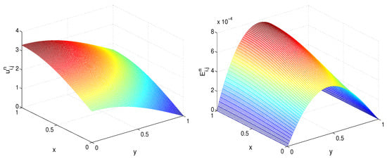
Figure 1.
Numerical solution u (left) and error (right) in the spatial computational domain, where , , and (Example 1).
Example 2.
Now, we set
We present the computational results for and in Table 3 and Table 4, respectively. The accuracy of the recovered source q is , and the accuracy of the solution u is .
Table 3.
Errors and convergence rates of the numerically recovered function q and solution u, where (Example 2).
Table 4.
Errors and convergence rates of the numerically recovered solution u, where (Example 2).
We plotted the numerical solution u and the error in Figure 2.
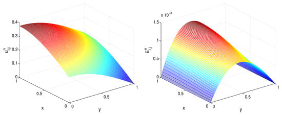
Figure 2.
Numerical solution u (left) and error (right) in the spatial computational domain, where , , and (Example 2).
Example 3.
We consider the inverse problem in Equations (1)–(7) for identifying the source and the solution with the following input data:
Now, the exact solution is not known.
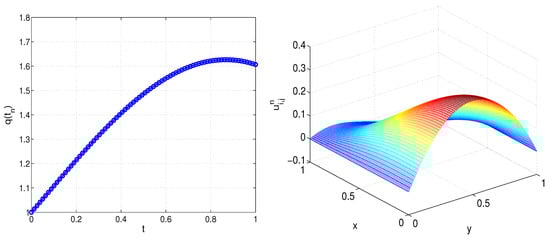
Figure 3.
Recovered solution q (left) and u (right) at final time, where and (Example 3).
8. Conclusions
In this paper, we investigated an inverse source initial-boundary value problem for the linear two-dimensional diffusion equation. The problem was formulated both with Dirichlet and Neumann boundary conditions, and a solution integral constraint governed the determination of the time-dependent source. Unlike many existing studies that focused on estimating the source within either the differential operator or the boundary conditions, we derived a priori estimates of the solution and the unknown source in a strong norm. Furthermore, the existence and uniqueness of a classical solution to the inverse problem were rigorously proven.
Using the structure of the boundary conditions, we reduced the original two-dimensional inverse source problem to an equivalent one-dimensional formulation. We first proved the well posedness of the inverse problem and then derived a series of a priori estimates for the solution and source term. In the final part of this process, the existence and uniqueness of a classical solution to the inverse problem were proven.
To support the theoretical analysis and provide a complete investigation, we presented a numerical method for solving the inverse problem. The proposed scheme is second-order accurate in space and first-order accurate in time. The computational results demonstrated the convergence of the numerical solution to the exact solution.
In our future work, we aim to extend both the theoretical framework and numerical approach to more complex two-dimensional convection-diffusion parabolic problems.
Author Contributions
Conceptualization, L.G.V. and M.N.K.; methodology, M.N.K. and L.G.V.; investigation, M.N.K. and L.G.V.; resources, M.N.K. and L.G.V.; writing—original draft preparation, M.N.K. and L.G.V.; writing—review and editing, L.G.V.; validation, M.N.K. All authors have read and agreed to the published version of the manuscript.
Funding
This study is financed by the European Union-NextGenerationEU through the National Recovery and Resilience Plan of the Republic of Bulgaria, project number BG-RRP-2.013-0001.
Institutional Review Board Statement
Not applicable.
Informed Consent Statement
Not applicable.
Data Availability Statement
Data are contained within the article.
Acknowledgments
The authors are very grateful to the anonymous reviewers, whose valuable comments and suggestions improved the quality of this paper.
Conflicts of Interest
The authors declare no conflicts of interest.
References
- Beck, J.V.; Blackwell, B.; Clair, C.R.S. Inverse Heat Conduction: Ill-Posed Problems; A Wiley-Interscience Publication: New York, NY, USA, 1985. [Google Scholar]
- Capasso, V.; Kunisch, K. A reaction-diffusion system arising in modelling man-environment diseases. J. Q. Appl. Math. 1988, 46, 431–450. [Google Scholar] [CrossRef]
- Crank, J. The Mathematics of Diffusion, 2nd ed.; Clarendon Press: Oxford, UK, 1975. [Google Scholar]
- Koleva, M.N.; Vulkov, L.G. Numerical method for space degenerate fractional derivative problems of atmospheric pollution. AIP Conf. Proc 2022, 2505, 080024. [Google Scholar]
- Koleva, M.N.; Vulkov, L.G. Positivity-preserving finite volume difference schemes for atmospheric dispersion models with degenerate vertical diffusion. Comput. Appl. Math. 2022, 41, 406. [Google Scholar] [CrossRef]
- Koleva, M.N.; Vulkov, L.G. Reconstruction coefficient analysis of honeybee collapse due to pesticide contamination. J. Phys. Conf. Ser. 2023, 2675, 012024. [Google Scholar] [CrossRef]
- Lesnic, D. Inverse Problems with Applications in Science and Engineering; CRC Press: Abingdon, UK, 2021; p. 349. [Google Scholar]
- Cannon, J.R.; Lin, Y.; Matheson, A.L. The solution of the diffusion equation in two-space variables subject to the specification of mass. Appl. Anal. 1993, 50, 1–15. [Google Scholar] [CrossRef]
- Hinze, M.; Pinnau, R.; Ulbrich, M.; Ulbrich, S. Optimization with PDE Constraints, 1st ed.; Springer: Dordrecht, The Netherlands, 2008; 270p. [Google Scholar]
- Ngoma, S. Inverse Source Problem and Inverse Diffusion Coeffcient Problem for Parabolic Equations with Applications in Geology. Doctoral Dissertation, Auburn University, Auburn, AL, USA, 2017. [Google Scholar]
- Woodbury, K.A.; Najafi, H.; de Monte, F.; Beck, J.V. Iverse Heat Conduction: Ill-Posed Problems, 2nd ed.; John Wiley & Sons, Inc.: Hoboken, NJ, USA, 2023. [Google Scholar]
- Chachuat, B.C. Nonlinear and Dynamic Optimization: From Theory to Practice; LA-TEACHING-2007-001; École Polytechnique Fédeérale de Lausanne: Lausanne, Switzerland, 2007. [Google Scholar]
- Malmir, I. Pure fractional optimal control of partial differential equations: Nonlinear, delay and two-dimensional PDEs. Pan-Am. J. Math. 2025, 4, 9. [Google Scholar] [CrossRef]
- Malmir, I. New pure multi-order fractional optimal control problems with constraints: QP and LP methods. ISA Trans. 2024, 153, 155–190. [Google Scholar] [CrossRef]
- Ladyženskaja, O.A.; Solonnikov, V.A.; Ural’ceva, N.N. Linear and Quasi-Linear Equations of Parabolic Type; Transl. Math. Monogr.; American Matematical Society: Providence, RI, USA, 1988; Volume 23. [Google Scholar]
- Hasanov, A.H.; Romanov, V.G. Introduction to Inverse Problems for Differential Equations, 1st ed.; Springer: Cham, Switzerland, 2017; 261p. [Google Scholar]
- Isakov, V. Inverse Problems for Partial Differential Equations, 3rd ed.; Springer: Cham, Switzerland, 2017; p. 406. [Google Scholar]
- Kabanikhin, S.I. Inverse and Ill-Posed Problems; DeGruyer: Berlin, Germany, 2011. [Google Scholar]
- Prilepko, A.I.; Orlovsky, D.G.; Vasin, I.A. Methods for Solving Inverse Problems in Mathematical Physics; Marcel Dekker: New York, NY, USA, 2000. [Google Scholar]
- Samarskii, A.A.; Vabishchevich, P.N. Numerical Methods for Solving Inverse Problems in Mathematical Physics; de Gruyter: Berlin, Germany, 2007; 438p. [Google Scholar]
- Gayte Delgado, I.; Marin-Gayte, I. A new method for the exact controllability of linear parabolic equations. Mathematics 2025, 13, 344. [Google Scholar] [CrossRef]
- Oanh, N.T.N. Source identification for parabolic equations from integral observations by the finite difference splitting method. Acta Math. Vietnam. 2024, 49, 283–308. [Google Scholar] [CrossRef]
- Sharma, T.; Beilina, L.; Sakthivel, K. Reconstruction of source function in a parabolic equation using partial boundary measurements. arXiv 2025, arXiv:2504.16070. [Google Scholar]
- Hasanov, A.; Slodicka, M. An analysis of inverse source problems with final time measured output data for the heat conduction equation: A semigroup approach. Appl. Math. Lett. 2013, 26, 207–214. [Google Scholar] [CrossRef]
- Liu, K.; Zhao, Y. Inverse moving source problems for parabolic equations. Appl. Math. Lett. 2024, 155, 109114. [Google Scholar] [CrossRef]
- Koleva, M.N.; Vulkov, L.G. Numerical determination of source from point observation in a time-fractional boundary-value problem on disjoint intervals. In Large-Scale Scientific Computations. LSSC 2023; Lirkov, I., Margenov, S., Eds.; Lecture Notes in Computer Science; Springer: Cham, Swizterland, 2024; Volume 13952, pp. 137–145. [Google Scholar]
- Kamynin, V.L. On the solvability of the inverse problem for determining the right-hand side of a degenerate parabolic equation with integral observation. Math. Notes 2015, 98, 765–777. [Google Scholar] [CrossRef]
- Kamynin, V.L. The inverse problem of recovering the source function in a multidimensional nonuniformly parabolic equation. Math. Notes 2022, 112, 412–423. [Google Scholar] [CrossRef]
- Kamynin, V.L.; Bukharova, T.I. Inverse problems of determination of the right-hand side term in the degenerate higher-order parabolic equation on a plane. In Numerical Analysis and Its Applications. NAA 2016; Dimov, I., Faragó, I., Vulkov, L., Eds.; Lecture Notes in Computer Science; Springer: Cham, Swizterland, 2017; Volume 10187, pp. 391–397. [Google Scholar]
- Kamynin, V.L. The inverse problem of the simultaneous determination of the right-hand side and the lowest coefficient in parabolic equations with many space variables. Math. Notes 2015, 97, 349–361. [Google Scholar] [CrossRef]
- Ivanchov, M.; Vlasov, V. Inverse problem for a 2D strongly degenerate heat equation with integral overdetermination conditions. Bukovinian Math. J. 2019, 7, 3–47. [Google Scholar]
- Koleva, M.N.; Vulkov, L.G. A Galerkin finite element method for the reconstruction of a time-dependent convection coefficient and source in a 1D model of magnetohydrodynamics. Appl. Sci. 2024, 14, 5949. [Google Scholar] [CrossRef]
- Dehghang, M. Saul’yev techniques for solving a parabolic equations with a nonlinear boundary specification, Intern. J. Comput. Math. 2003, 80, 257–265. [Google Scholar]
- Dehghan, M. A finite difference method for a non-local boundary value problem for two-dimensional heat equation. Appl. Math. Comput. 2000, 112, 133–142. [Google Scholar] [CrossRef]
- Koleva, M.N.; Vulkov, L.G. Numerical determination of a time-dependent boundary condition for a pseudoparabolic equation from integral observation. Computation 2024, 12, 243. [Google Scholar] [CrossRef]
- Koleva, M.N.; Vulkov, L.G. Numerical reconstruction of time-dependent boundary conditions to 2D heat equation on disjoint rectangles at integral observations. Mathematics 2024, 12, 1499. [Google Scholar] [CrossRef]
- Dehghan, M. A new ADI technique for two-dimensional parabolic equation with an integral condition. Comput. Math. Appl. 2002, 43, 1477–1488. [Google Scholar] [CrossRef]
- Merazga, N.; Bouziani, A. Rothe method for a mixed problem with an integral condition for the two-dimensional diffusion equation. Abstr. Appl. Anal. 2003, 2003, 899–922. [Google Scholar] [CrossRef]
- Evans, L.C. Partial Differential Equations, 2nd ed.; American Mathematical Society: Providence, RI, USA, 2010. [Google Scholar]
- Bondarev, E.A.; Voevodin, A.F. A finite difference method for solving initial-boundary value problems for loaded differential and integro-differential equations. Differ. Equ. 2000, 36, 1711–1714. [Google Scholar] [CrossRef]
Disclaimer/Publisher’s Note: The statements, opinions and data contained in all publications are solely those of the individual author(s) and contributor(s) and not of MDPI and/or the editor(s). MDPI and/or the editor(s) disclaim responsibility for any injury to people or property resulting from any ideas, methods, instructions or products referred to in the content. |
© 2025 by the authors. Licensee MDPI, Basel, Switzerland. This article is an open access article distributed under the terms and conditions of the Creative Commons Attribution (CC BY) license (https://creativecommons.org/licenses/by/4.0/).