Sine Unit Exponentiated Half-Logistic Distribution: Theory, Estimation, and Applications in Reliability Modeling

Abstract

This study introduces the sine unit exponentiated half-logistic distribution, a novel extension of the unit exponentiated half-logistic distribution within the sine-G family. Using trigonometric transformations, the proposed distribution offers flexible density shapes for modeling asymmetric unit-interval data. We derive its statistical properties, including quantiles, moments, and stress–strength reliability, and estimate parameters via classical methods like maximum likelihood and Anderson–Darling. Simulations and real-world applications to fiber strength and burr datasets demonstrate the superior fit of the proposed distribution over competing models, highlighting its utility in reliability engineering and manufacturing.

1. Introduction

The increasing complexity of modern datasets, characterized by diverse and asymmetric patterns, underscores the need for flexible statistical models capable of capturing intricate data structures. Traditional probability distributions often fall short in modeling dynamic or heterogeneous data, prompting the development of innovative distributions to address these challenges. This limitation has driven researchers to create adaptable models tailored to the evolving demands of real-world data. Consequently, the statistical community has focused on enhancing distribution theory to better fit complex empirical datasets.

To tackle the challenges posed by complex data, researchers have developed generated families of distributions that enhance traditional models through transformations or parameter expansions [1,2,3]. These families provide greater flexibility, enabling the modeling of heavy-tailed or skewed datasets prevalent in reliability and survival analysis [4,5]. Techniques such as modifying failure rates, density functions, or applying trigonometric transformations allow new distributions to capture underlying data patterns effectively [6,7]. Such approaches offer a robust framework for overcoming the constraints of classical distributions, paving the way for advanced statistical modeling [8].

The need to model intricate empirical data has spurred significant advancements in distribution theory, particularly for datasets exhibiting heterogeneity and asymmetry. Classical models often fail to reflect the diverse dynamics of contemporary datasets, necessitating sophisticated generated families designed through innovative transformations [9,10,11]. Notable examples include the sine-G family for trigonometric modeling [10,12,13] and exponentiated sine-G for reliability applications [14]. Half-logistic-based families have also gained prominence, such as the beta half-logistic [15], half-logistic xgamma [16], and unit-exponentiated half-logistic [17,18,19,20,21]. Further extensions include the modified half-logistic [22], gamma power half-logistic [23], and half-logistic Kies exponential [24]. Bounded-domain models, such as the odd log-logistic-G [25] and exponentiated Fréchet [26,27], enhance flexibility for unit-interval data. Reliability modeling is advanced through stress–strength analyses [28] and Kumaraswamy-G [29]. Additive models effectively capture bathtub-shaped hazard rates prevalent in reliability engineering [30,31,32,33,34,35]. These models are often combined with half-logistic distributions to enhance flexibility for asymmetric reliability data [36]. Parameter estimation techniques, including maximum likelihood and product-of-spacings methods, ensure accurate fitting of these models to empirical data [37,38,39,40,41,42]. These families collectively provide tailored solutions for complex data structures [43,44,45]. Despite these advancements, existing unit-interval distributions, such as Beta and Topp–Leone, often lack the flexibility to model asymmetric data in reliability engineering [18]. The proposed sine unit exponentiated half-logistic (SUEHL) distribution, inspired by the sine power half-logistic model [13], fills this gap by extending the unit exponentiated half-logistic (UEHL) distribution with trigonometric transformations. This two-parameter model offers diverse density shapes and robust reliability measures, including stress–strength reliability, inverse hazard rate, and mean residual life, making it a powerful tool for reliability applications [11,30].

Building on these developments, this study introduces the SUEHL distribution, a novel extension of the UEHL distribution within the sine-G family. Leveraging trigonometric transformations, the SUEHL enhances flexibility for modeling asymmetric unit-interval data, drawing inspiration from recent trigonometric models. The manuscript explores its statistical properties, estimation methods, and real-world applications, demonstrating its utility in reliability engineering and manufacturing. The subsequent sections are organized as follows: Section 2 defines the SUEHL distribution, Section 3 derives its properties, Section 4 discusses estimation, Section 5 presents simulations, Section 6 provides real-data applications, and Section 7 concludes with future directions.

2. Description of the Model

Recently, Özbilen and Genç [18] developed the UEHL distribution, grounded in the omega distribution and categorized within the proportional hazard rate model framework. The cumulative distribution function (CDF) of the UEHL distribution is defined as

$$F_{UEHL}\left(x\mid \theta ,\lambda \right)=1-{\left({\displaystyle \frac{1-x^{\theta }}{1+x^{\theta }}}\right)}^{\lambda },0<x<1,$$

(1)

with corresponding probability distribution function (PDF)

$$f_{UEHL}\left(x\mid \theta ,\lambda \right)=2\lambda \theta x^{\theta -1}{\displaystyle \frac{{\left(1-x^{\theta }\right)}^{\lambda -1}}{{\left(1+x^{\theta }\right)}^{\lambda +1}}},0<x<1,$$

where $\theta >0$ and $\lambda >0$ are the shape parameters. The UEHL distribution demonstrates multiple applications in reliability theory, leveraging the exponentiated half-logistic distribution [11,18].

In this section, a novel and flexible distribution, termed the SUEHL, is introduced by integrating the CDF of the UEHL distribution into the sine-G family framework. The CDF of the sine-G family of distributions is defined as

$$G\left(t;\zeta \right)=sin\left({\displaystyle \frac{1}{2}}\pi F\left(t;\zeta \right)\right),-\infty <t<\infty$$

(2)

where $F\left(t;\zeta \right)$ is the baseline CDF of a continuous distribution and $\zeta$ is the parameter vector of the distribution. The approach can be used to leverage the trigonometric transformation to enhance the adaptability of the baseline UEHL model. The CDF of the SUEHL distribution is obtained by substituting $F_{UEHL}(x\mid \theta ,\lambda )$ from Equation (1) into the sine-G family transformation in Equation (2), yielding

$$F(x\mid \theta ,\lambda )=cos\left({\displaystyle \frac{\pi }{2}}{\left({\displaystyle \frac{1-x^{\theta }}{1+x^{\theta }}}\right)}^{\lambda }\right),0<x<1,$$

(3)

where $\theta ,\lambda >0$ are the shape parameters. The corresponding probability density function (PDF) of the SUEHL distribution is obtained by differentiating the CDF (3), given by

$$f(x\mid \theta ,\lambda )=\pi \lambda \theta x^{\theta -1}\left({\displaystyle \frac{{(1-x^{\theta })}^{\lambda -1}}{{(1+x^{\theta })}^{\lambda +1}}}\right)sin\left({\displaystyle \frac{\pi }{2}}{\left({\displaystyle \frac{1-x^{\theta }}{1+x^{\theta }}}\right)}^{\lambda }\right),0<x<1,\theta ,\lambda >0.$$

(4)

The SUEHL distribution exhibits remarkable flexibility in capturing various density shapes within the unit interval $(0,1)$. Specifically, the PDF can display positively skewed, reverse J-shaped, U-shaped, or unimodal configurations, depending on the parameter values. The behaviors are illustrated in the top row in Figure 1, which visualizes the density for different parameter combinations. To visualize the behavior of the distribution in the three-dimensional case, we present the second and third rows of Figure 1 for specific parameter values while keeping the other parameter fixed. For the special case where $\lambda =1$, the PDF simplifies to a sine-transformed version of the unit half-logistic distribution, serving as a new sub-model. Also, the survival function (SF) and hazard rate function (HRF) of the SUEHL distribution are derived as

$$S(x\mid \theta ,\lambda )=1-cos\left({\displaystyle \frac{\pi }{2}}{\left({\displaystyle \frac{1-x^{\theta }}{1+x^{\theta }}}\right)}^{\lambda }\right),0<x<1,\theta ,\lambda >0$$

(5)

and

$$h(x\mid \theta ,\lambda )=\pi \theta \lambda x^{\theta -1}{\displaystyle \frac{{(1-x^{\theta })}^{\lambda -1}}{{(1+x^{\theta })}^{\lambda +1}}}{\displaystyle \frac{sin\left(\frac{\pi }{2}{\left(\frac{1-x^{\theta }}{1+x^{\theta }}\right)}^{\lambda }\right)}{1-cos\left(\frac{\pi }{2}{\left(\frac{1-x^{\theta }}{1+x^{\theta }}\right)}^{\lambda }\right)}},0<x<1,\theta ,\lambda >0.$$

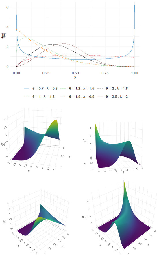
Figure 1. SUEHL probability density function for various parameter values.

3. Some Statistical Characteristics

3.1. Quantile Function

The quantile function of a statistical distribution provides a critical tool for generating random variates and understanding the distributional properties across different probability levels. The quantile function of the SUEHL distribution is

$$Q(p\mid \theta ,\lambda )={\left({\displaystyle \frac{1-{\left(\frac{2}{\pi }{cos}^{-1}\left(p\right)\right)}^{1/\lambda }}{1+{\left(\frac{2}{\pi }{cos}^{-1}\left(p\right)\right)}^{1/\lambda }}}\right)}^{1/\theta },p\in (0,1).$$

(6)

Some numerical values of the quantiles of the proposed SUEHL model are presented in Table 1.

Table 1. Some numerical values for the quantiles of the proposed model.

$\mathit{\theta }$	$\mathit{\lambda }$	$\mathit{Q}\left(0.05\right)$	$\mathit{Q}\left(0.1\right)$	$\mathit{Q}\left(0.2\right)$	$\mathit{Q}\left(0.3\right)$	$\mathit{Q}\left(0.5\right)$	$\mathit{Q}\left(0.7\right)$	$\mathit{Q}\left(0.9\right)$	$\mathit{Q}\left(0.99\right)$
0.5	0.5	0.00105	0.00433	0.01859	0.04510	0.14793	0.35028	0.71854	0.96804
	1	0.00026	0.00108	0.00469	0.01154	0.04000	0.10739	0.30674	0.69669
	2	0.00006	0.00027	0.00118	0.00290	0.01021	0.02839	0.09133	0.28971
	4	0.00002	0.00007	0.00029	0.00073	0.00256	0.00720	0.02394	0.08531
	6	0.00001	0.00003	0.00013	0.00032	0.00114	0.00321	0.01073	0.03917
	8	0.00000	0.00002	0.00007	0.00018	0.00064	0.00181	0.00606	0.02229
1	0.5	0.03235	0.06580	0.13633	0.21236	0.38461	0.59184	0.84767	0.98389
	1	0.01618	0.03293	0.06848	0.10740	0.20000	0.32770	0.55384	0.83468
	2	0.00809	0.01647	0.03428	0.05386	0.10102	0.16850	0.30221	0.53825
	4	0.00404	0.00824	0.01715	0.02695	0.05064	0.08486	0.15472	0.29209
	6	0.00270	0.00549	0.01143	0.01797	0.03378	0.05665	0.10361	0.19792
	8	0.00202	0.00412	0.00857	0.01348	0.02534	0.04251	0.07783	0.14930
2	0.5	0.17986	0.25651	0.36923	0.46082	0.62017	0.76931	0.92069	0.99191
	1	0.12720	0.18148	0.26169	0.32772	0.44721	0.57245	0.74421	0.91361
	2	0.08995	0.12834	0.18515	0.23207	0.31784	0.41049	0.54974	0.73366
	4	0.06360	0.09076	0.13094	0.16416	0.22503	0.29130	0.39335	0.54045
	6	0.05193	0.07410	0.10692	0.13404	0.18378	0.23801	0.32189	0.44488
	8	0.04497	0.06417	0.09259	0.11609	0.15917	0.20617	0.27898	0.38639
3	0.5	0.31864	0.40371	0.51467	0.59661	0.72724	0.83959	0.94640	0.99460
	1	0.25292	0.32054	0.40913	0.47534	0.58480	0.68943	0.82122	0.94154
	2	0.20075	0.25444	0.32486	0.37764	0.46573	0.55233	0.67107	0.81344
	4	0.15934	0.20195	0.25786	0.29981	0.36997	0.43944	0.53685	0.66349
	6	0.13919	0.17642	0.22527	0.26192	0.32325	0.38405	0.46968	0.58277
	8	0.12647	0.16029	0.20467	0.23797	0.29371	0.34899	0.42696	0.53050
5	0.5	0.50348	0.58029	0.67130	0.73352	0.82605	0.90041	0.96749	0.99676
	1	0.43832	0.50528	0.58495	0.64004	0.72478	0.80001	0.88854	0.96450
	2	0.38159	0.43989	0.50935	0.55751	0.63224	0.70036	0.78716	0.88348
	4	0.33219	0.38295	0.44344	0.48541	0.55068	0.61057	0.68851	0.78181
	6	0.30632	0.35313	0.40890	0.44761	0.50783	0.56317	0.63545	0.72326
	8	0.28919	0.33338	0.38604	0.42259	0.47946	0.53173	0.60011	0.68361
10	0.5	0.70956	0.76177	0.81933	0.85646	0.90887	0.94890	0.98361	0.99838
	1	0.66206	0.71083	0.76482	0.80002	0.85134	0.89443	0.94262	0.98209
	2	0.61773	0.66324	0.71369	0.74666	0.79514	0.83687	0.88722	0.93994
	4	0.57636	0.61883	0.66591	0.69671	0.74208	0.78139	0.82977	0.88420
	6	0.55346	0.59424	0.63945	0.66904	0.71262	0.75044	0.79715	0.85045
	8	0.53776	0.57739	0.62132	0.65007	0.69243	0.72920	0.77467	0.82681

Table 1 shows that, for a fixed $\theta$, increasing $\lambda$ results in smaller quantile values, indicating a concentration of the distribution around lower values. Conversely, for a fixed $\lambda$, increasing $\theta$ shifts the quantiles to the right, suggesting a broader spread and heavier tail toward higher values.

3.2. Moments

Studying the moments of a random variable provides valuable insights into several characteristics of its distribution. In this section, we derive the series expansions for the n-th moment of the SUEHL distribution. The Taylor series expansion of the sine function, used in the derivation, is given by

$$\sin (t)=\sum _{j=0}^{\infty }{\displaystyle \frac{{(-1)}^j}{(2j+1)!}}{t}^{2j+1},$$

(7)

Let X follow an SUEHL distribution with parameters $\theta$ and $\lambda$. The n-th moment of the random variable X is

$$E\left(X^n\right)={\int }_0^1{x}^n·\pi \lambda \theta x^{\theta -1}\left({\displaystyle \frac{{(1-x^{\theta })}^{\lambda -1}}{{(1+x^{\theta })}^{\lambda +1}}}\right)sin\left({\displaystyle \frac{\pi }{2}}{\left({\displaystyle \frac{1-x^{\theta }}{1+x^{\theta }}}\right)}^{\lambda }\right)dx,$$

which simplifies to

$$E\left(X^n\right)=\pi \lambda \theta {\int }_0^1{x}^{n+\theta -1}\left({\displaystyle \frac{{(1-x^{\theta })}^{\lambda -1}}{{(1+x^{\theta })}^{\lambda +1}}}\right)sin\left({\displaystyle \frac{\pi }{2}}{\left({\displaystyle \frac{1-x^{\theta }}{1+x^{\theta }}}\right)}^{\lambda }\right)dx.$$

(8)

To derive the moments in Equation (8), we employ the Taylor series expansion of the sine function given in Equation (7) and substitute $t={\displaystyle \frac{\pi }{2}}{\left({\displaystyle \frac{1-x^{\theta }}{1+x^{\theta }}}\right)}^{\lambda }$, which yields

$$\begin{array}{c}\hfill E\left(X^n\right)=\pi \lambda \theta \sum _{j=0}^{\infty }{\displaystyle \frac{{(-1)}^j}{(2j+1)!}}{\left({\displaystyle \frac{\pi }{2}}\right)}^{2j+1}{\int }_0^1{x}^{n+\theta -1}{\displaystyle \frac{{(1-x^{\theta })}^{2\lambda j+2\lambda -1}}{{(1+x^{\theta })}^{2\lambda j+2\lambda +1}}}dx.\end{array}$$

(9)

Substituting $x=u^{1/\theta }$ and applying the binomial series expansion, the integral in Equation (9) is evaluated by

$$E\left(X^n\right)=\pi \lambda \sum _{j=0}^{\infty }\sum _{i=0}^{\infty }\left({\displaystyle \genfrac{}{}{0pt}{}{2\lambda j+2\lambda +i}{i}}\right){\displaystyle \frac{{(-1)}^{i+j}}{(2j+1)!}}{\left({\displaystyle \frac{\pi }{2}}\right)}^{2j+1}B\left({\displaystyle \frac{n}{\theta }}+i+1;2\lambda j+2\lambda \right),$$

where $B(a;b)$ is the beta function. This expression provides an explicit analytic form for the moments.

3.3. Reliability Analysis

This section explores the reliability properties of the SUEHL distribution, including stress–strength reliability, inverse hazard rate function (IHRF), and mean residual life (MRL), complementing the hazard rate function provided in Equation (4).

3.3.1. Stress–Strength Reliability

The stress–strength reliability model describes the operational lifespan of a component subjected to random stress and possessing random strength. Let $X_1$ represent the strength and $X_2$ the applied stress, where failure occurs if $X_2>X_1$, and the component functions when $X_1>X_2$. For the SUEHL distribution, we assume $X_1\sim \mathrm{SUEHL}(\theta ,{\lambda }_1)$ and $X_2\sim \mathrm{SUEHL}(\theta ,{\lambda }_2)$ with a common shape parameter $\theta$. The stress–strength reliability, $R=P(X_1>X_2)$, is computed as

$$R={\int }_0^1\pi {\lambda }_2\theta y^{\theta -1}\left({\displaystyle \frac{{(1-y^{\theta })}^{{\lambda }_2-1}}{{(1+y^{\theta })}^{{\lambda }_2+1}}}\right)sin\left({\displaystyle \frac{\pi }{2}}{\left({\displaystyle \frac{1-y^{\theta }}{1+y^{\theta }}}\right)}^{{\lambda }_2}\right)cos\left({\displaystyle \frac{\pi }{2}}{\left({\displaystyle \frac{1-y^{\theta }}{1+y^{\theta }}}\right)}^{{\lambda }_1}\right)dy.$$

(10)

The integral in Equation (10) represents the probability that $X_1>y$ for all possible values of $X_2=y$. To evaluate the integral, we apply series expansions

$$\begin{array}{c}\hfill R={\int }_0^1\pi {\lambda }_2\theta y^{\theta -1}\left[\sum _{j=0}^{\infty }{\displaystyle \frac{{(-1)}^j}{(2j+1)!}}{\left({\displaystyle \frac{\pi }{2}}\right)}^{2j+1}{\left({\displaystyle \frac{1-y^{\theta }}{1+y^{\theta }}}\right)}^{(2j+1){\lambda }_2}\right]\left[\sum _{i=0}^{\infty }{\displaystyle \frac{{(-1)}^i}{\left(2i\right)!}}{\left({\displaystyle \frac{\pi }{2}}\right)}^{2i}{\left({\displaystyle \frac{1-y^{\theta }}{1+y^{\theta }}}\right)}^{2i{\lambda }_1}\right]dy\\ \hfill =\pi {\lambda }_2\theta \sum _{i=0}^{\infty }\sum _{j=0}^{\infty }{\displaystyle \frac{{(-1)}^{i+j}}{\left(2i\right)!(2j+1)!}}{\left({\displaystyle \frac{\pi }{2}}\right)}^{2i+2j+1}{\int }_0^1{y}^{\theta -1}{\displaystyle \frac{{(1-y^{\theta })}^{2i{\lambda }_1+(2j+1){\lambda }_2-1}}{{(1+y^{\theta })}^{2i{\lambda }_1+(2j+1){\lambda }_2+1}}}dy,\end{array}$$

where $I_{i,j}$ is defined as

$$I_{i,j}={\int }_0^1{y}^{\theta -1}{\displaystyle \frac{{(1-y^{\theta })}^{2i{\lambda }_1+(2j+1){\lambda }_2-1}}{{(1+y^{\theta })}^{2i{\lambda }_1+(2j+1){\lambda }_2+1}}}dy.$$

Substituting $t=y^{\theta }$ and using the binomial series expansion, we obtain

$$I_{i,j}={\displaystyle \frac{1}{\theta }}\sum _{k=0}^{\infty }{(-1)}^k\left({\displaystyle \genfrac{}{}{0pt}{}{2i{\lambda }_1+(2j+1){\lambda }_2+k}{k}}\right)B(2i{\lambda }_1+(2j+1){\lambda }_2;k+1).$$

Thus, the stress–strength reliability is

$$\begin{array}{c}\hfill R={\displaystyle \frac{\pi {\lambda }_2}{\theta }}\sum _{i=0}^{\infty }\sum _{j=0}^{\infty }\sum _{k=0}^{\infty }{\displaystyle \frac{{(-1)}^{i+j+k}}{\left(2i\right)!(2j+1)!k!}}{\left({\displaystyle \frac{\pi }{2}}\right)}^{2i+2j+1}\\ \hfill \times \left({\displaystyle \genfrac{}{}{0pt}{}{2i{\lambda }_1+(2j+1){\lambda }_2+k}{k}}\right)B(2i{\lambda }_1+(2j+1){\lambda }_2;k+1).\end{array}$$

(11)

The expression in Equation (11) facilitates computing the reliability for practical applications.

3.3.2. Inverse Hazard Rate and Mean Residual Life

To further characterize the SUEHL’s reliability, we derive the inverse hazard rate function (IHRF) and mean residual life (MRL). The IHRF is defined as $h_I\left(x\right)={\displaystyle \frac{f\left(x\right)}{F\left(x\right)}}$, where $f\left(x\right)$ is the PDF and $F\left(x\right)$ is the CDF of the relevant distribution. For the SUEHL distribution, it is given by

$$h_I(x\mid \theta ,\lambda )=\pi \lambda \theta x^{\theta -1}{\displaystyle \frac{{(1-x^{\theta })}^{\lambda -1}}{{(1+x^{\theta })}^{\lambda +1}}}{\displaystyle \frac{sin\left(\frac{\pi }{2}{\left(\frac{1-x^{\theta }}{1+x^{\theta }}\right)}^{\lambda }\right)}{cos\left(\frac{\pi }{2}{\left(\frac{1-x^{\theta }}{1+x^{\theta }}\right)}^{\lambda }\right)}},0<x<1,\theta ,\lambda >0.$$

This function characterizes the probability of immediate failure given survival up to time x, offering insights into reliability for small time increments.

The MRL function represents the expected remaining lifetime given survival past x. It is defined as

$$m(x\mid \theta ,\lambda )={\displaystyle \frac{1}{S\left(x\right)}}{\int }_x^1(t-x)f(t\mid \theta ,\lambda )dt,0<x<1,\theta ,\lambda >0,$$

(12)

where $S\left(x\right)$ is the survival function and $f(t\mid \theta ,\lambda )$ is the PDF. To compute the MRL in Equation (12), we derive its series expansion using the Taylor series of the PDF’s sine term given by Equation (7). The resulting form is

$$m(x\mid \theta ,\lambda )={\displaystyle \frac{\pi \lambda \theta }{S\left(x\right)}}\sum _{j=0}^{\infty }{\displaystyle \frac{{(-1)}^j}{(2j+1)!}}{\left({\displaystyle \frac{\pi }{2}}\right)}^{2j+1}{\displaystyle \frac{1}{\theta }}\sum _{k=0}^{\infty }{(-1)}^k\left({\displaystyle \genfrac{}{}{0pt}{}{(2j+1)\lambda +k}{k}}\right)\left[B\left(x^{\theta };{\displaystyle \frac{1}{\theta }}+k+1,(2j+1)\lambda \right)-xB\left(x^{\theta };{\displaystyle \frac{1}{\theta }}+k,(2j+1)\lambda \right)\right],$$

where $B(z;a,b)$ is the incomplete beta function. This series facilitates numerical evaluation and provides a practical measure for reliability applications, such as predicting component longevity in engineering systems.

3.4. Information Measures

To analyze the uncertainty associated with the SUEHL distribution, we derive the Shannon entropy and residual entropy, providing insights into its information content.

The Shannon entropy, measuring the expected uncertainty, is defined as

$$H\left(X\right)=-{\int }_0^{1}f(x\mid \theta ,\lambda )logf(x\mid \theta ,\lambda )dx,$$

where $f(x\mid \theta ,\lambda )$ is the PDF. Decomposing $logf\left(x\right)$ into five terms and using the series expansion of the sine term in Equation (7), we express the entropy as

$$H\left(X\right)\approx -log\left(\pi \lambda \theta \right)-(\theta -1)T_1+(\lambda -1)T_2-(\lambda +1)T_3+T_4,$$

$$\begin{array}{cc}\hfill T_1& =\pi \lambda \sum _{j=0}^{\infty }{\displaystyle \frac{{(-1)}^j}{(2j+1)!}}{\left({\displaystyle \frac{\pi }{2}}\right)}^{2j+1}\sum _{k=0}^{\infty }{(-1)}^k\left({\displaystyle \genfrac{}{}{0pt}{}{(2j+1)\lambda +k}{k}}\right)\hfill \\ \hfill & \times B\left({\displaystyle \frac{1}{\theta }}+k,(2j+1)\lambda \right)\left(\psi \left({\displaystyle \frac{1}{\theta }}+k\right)-\psi \left({\displaystyle \frac{1}{\theta }}+k+(2j+1)\lambda \right)\right),\hfill \end{array}$$

$$\begin{array}{cc}\hfill T_2& =\pi \lambda \sum _{j=0}^{\infty }{\displaystyle \frac{{(-1)}^j}{(2j+1)!}}{\left({\displaystyle \frac{\pi }{2}}\right)}^{2j+1}\sum _{k=0}^{\infty }{(-1)}^k\left({\displaystyle \genfrac{}{}{0pt}{}{(2j+1)\lambda +k}{k}}\right)\hfill \\ \hfill & \times B\left({\displaystyle \frac{1}{\theta }}+k,(2j+1)\lambda \right)\left(\psi \left((2j+1)\lambda \right)-\psi \left({\displaystyle \frac{1}{\theta }}+k+(2j+1)\lambda \right)\right),\hfill \end{array}$$

$$\begin{array}{cc}\hfill T_3& =\pi \lambda \sum _{j=0}^{\infty }{\displaystyle \frac{{(-1)}^j}{(2j+1)!}}{\left({\displaystyle \frac{\pi }{2}}\right)}^{2j+1}\sum _{k=0}^{\infty }\sum _{m=1}^{\infty }{\displaystyle \frac{{(-1)}^{k+m-1}}{m}}\hfill \\ \hfill & \times \left({\displaystyle \genfrac{}{}{0pt}{}{(2j+1)\lambda +k}{k}}\right)B\left({\displaystyle \frac{1}{\theta }}+m+k,(2j+1)\lambda \right),\hfill \end{array}$$

The residual entropy, measuring uncertainty given survival past x, is defined as

$$H(X\mid X>x)=-{\displaystyle \frac{1}{S\left(x\right)}}{\int }_x^{1}f(t\mid \theta ,\lambda )logf(t\mid \theta ,\lambda )dt,$$

where $S\left(x\right)$ is the survival function. The corresponding series expansion is

$$H(X\mid X>x)\approx -{\displaystyle \frac{1}{S\left(x\right)}}\left[\log (\pi \lambda \theta )(F\left(1\right)-F\left(x\right))+(\theta -1)T_1^{\prime }+(\lambda -1)T_2^{\prime }-(\lambda +1)T_3^{\prime }+T_4^{\prime }\right],$$

where $T_1^{\prime }$, $T_2^{\prime }$, and $T_3^{\prime }$ are analogous to $T_1$, $T_2$, $T_3$ with integrals from $x^{\theta }$ to 1 using the incomplete beta function $B(t^{\theta };a,b)$, and $T_4^{\prime }$ is evaluated numerically. This provides dynamic insights into the SUEHL’s uncertainty over time.

4. Estimation Methods

In this section, we explore various classical estimation techniques to estimate the parameters of the SUEHL distribution. We investigate several methods, including maximum likelihood (ML), Anderson–Darling (AD), ordinary and weighted least-squares (OLS and WLS), and Cramér–von Mises (CVM) [38,39,40], to enhance the straightforward nature of the estimation process with detailed derivations.

4.1. Maximum Likelihood Estimation

In this section, we estimate the SUEHL parameters using the maximum likelihood technique. Let $x_1,x_2,\dots ,x_n$ be an observed sample of size n from the PDF (4). The log-likelihood function is given by

$$\begin{array}{ccc}\hfill log\ell (\theta ,\lambda )& \propto & nlog\left(\pi \lambda \theta \right)+\sum _{i=1}^n(\theta -1)log{x}_i+\sum _{i=1}^n\left[(\lambda -1)log(1-x_i^{\theta })-(\lambda +1)log(1+x_i^{\theta })\right]\hfill \\ & & +\sum _{i=1}^{n}log\left[sin\left({\displaystyle \frac{\pi }{2}}{\left({\displaystyle \frac{1-x_i^{\theta }}{1+x_i^{\theta }}}\right)}^{\lambda }\right)\right]\hfill \end{array}$$

(13)

The ML estimators can be found by solving the partial differential equations corresponding to Equation (13) with respect to $\theta$ and $\lambda$:

$$\begin{array}{ccc}\hfill {\displaystyle \frac{\partial log\ell }{\partial \theta }}& =& {\displaystyle \frac{n}{\theta }}+\sum _{i=1}^{n}log{x}_i+\sum _{i=1}^n\left[(\lambda -1){\displaystyle \frac{-x_i^{\theta }log{x}_i}{1-x_i^{\theta }}}-(\lambda +1){\displaystyle \frac{x_i^{\theta }log{x}_i}{1+x_i^{\theta }}}\right]\hfill \\ & & -\sum _{i=1}^n{\displaystyle \frac{\pi \lambda }{2}}{\left({\displaystyle \frac{1-x_i^{\theta }}{1+x_i^{\theta }}}\right)}^{\lambda }cot\left({\displaystyle \frac{\pi }{2}}{\left({\displaystyle \frac{1-x_i^{\theta }}{1+x_i^{\theta }}}\right)}^{\lambda }\right){\displaystyle \frac{2x_i^{\theta }log{x}_i}{(1-x_i^{\theta })(1+x_i^{\theta })}}=0,\hfill \end{array}$$

(14)

$${\displaystyle \frac{\partial log\ell }{\partial \lambda }}={\displaystyle \frac{n}{\lambda }}+\sum _{i=1}^{n}log(1-x_i^{\theta })-\sum _{i=1}^{n}log(1+x_i^{\theta })+\sum _{i=1}^n{\displaystyle \frac{\pi }{2}}{\left({\displaystyle \frac{1-x_i^{\theta }}{1+x_i^{\theta }}}\right)}^{\lambda }cot\left({\displaystyle \frac{\pi }{2}}{\left({\displaystyle \frac{1-x_i^{\theta }}{1+x_i^{\theta }}}\right)}^{\lambda }\right)log\left({\displaystyle \frac{1-x_i^{\theta }}{1+x_i^{\theta }}}\right)=0.$$

(15)

Since Equations (14) and (15) have no explicit solutions due to the presence of trigonometric and logarithmic terms, numerical nonlinear techniques, such as the Newton–Raphson algorithm, must be employed to determine the MLEs of the SUEHL parameters.

4.2. Anderson–Darling Methods

The AD methods form a specialized class of minimum-distance estimators aimed at optimizing the fit of a distribution to empirical data. In this subsection, we derive three distinct estimators for the parameters of the SUEHL distribution: the Anderson–Darling Estimators (ADEs), Right-Tail Anderson–Darling Estimators (RTADEs), and Left-Tail Anderson–Darling Estimators (LTADEs). Let $x_{\left(1\right)},x_{\left(2\right)},\dots ,x_{\left(n\right)}$ represent the order statistics of a random sample drawn from the SUEHL distribution.

The Anderson-Darling Estimators (ADEs), denoted as ${\widehat{\theta }}_2$ and ${\widehat{\lambda }}_2$, are obtained by minimizing the following function with respect to the model parameters

$$A_1\left(\zeta \right)=-n-{\displaystyle \frac{1}{n}}\sum _{b=1}^n(2b-1)\left\{\log F(x_{\left(b\right)}\mid \zeta )+logS(x_{(n-b+1)}\mid \zeta )\right\},$$

where $F(·)$ is the CDF given by Equation (3), $S(·)$ is the survival function given by Equation (5), and $\zeta =(\theta ,\lambda )$. Alternatively, the ADEs can be determined by solving the following nonlinear system of equations:

$$\sum _{b=1}^n(2b-1)\left\{{\displaystyle \frac{v_{\zeta }(x_{\left(b\right)}\mid \zeta )}{F(x_{\left(b\right)}\mid \zeta )}}-{\displaystyle \frac{v_{\zeta }(x_{(n-b+1)}\mid \zeta )}{S(x_{(n-b+1)}\mid \zeta )}}\right\}=0,\zeta =(\theta ,\lambda ),$$

where the partial derivatives of the CDF are defined as

$$v_{\theta }(x_{\left(b\right)}\mid \zeta )={\displaystyle \frac{\partial F(x_{\left(b\right)}\mid \zeta )}{\partial \theta }}=-{\displaystyle \frac{\pi \lambda }{2}}{\left({\displaystyle \frac{1-x_{\left(b\right)}^{\theta }}{1+x_{\left(b\right)}^{\theta }}}\right)}^{\lambda -1}{\displaystyle \frac{2x_{\left(b\right)}^{\theta }log{x}_{\left(b\right)}}{{(1+x_{\left(b\right)}^{\theta })}^2}}sin\left({\displaystyle \frac{\pi }{2}}{\left({\displaystyle \frac{1-x_{\left(b\right)}^{\theta }}{1+x_{\left(b\right)}^{\theta }}}\right)}^{\lambda }\right),$$

(16)

$$v_{\lambda }(x_{\left(b\right)}\mid \zeta )={\displaystyle \frac{\partial F(x_{\left(b\right)}\mid \zeta )}{\partial \lambda }}=-{\displaystyle \frac{\pi }{2}}{\left({\displaystyle \frac{1-x_{\left(b\right)}^{\theta }}{1+x_{\left(b\right)}^{\theta }}}\right)}^{\lambda }log\left({\displaystyle \frac{1-x_{\left(b\right)}^{\theta }}{1+x_{\left(b\right)}^{\theta }}}\right)sin\left({\displaystyle \frac{\pi }{2}}{\left({\displaystyle \frac{1-x_{\left(b\right)}^{\theta }}{1+x_{\left(b\right)}^{\theta }}}\right)}^{\lambda }\right).$$

(17)

The RTADEs, denoted as ${\widehat{\theta }}_3$ and ${\widehat{\lambda }}_3$, are obtained by minimizing the function

$$A_2\left(\zeta \right)={\displaystyle \frac{n}{2}}-2\sum _{b=1}^{n}F(x_{\left(b\right)}\mid \theta ,\lambda )-{\displaystyle \frac{1}{n}}\sum _{b=1}^n(2b-1)logS(x_{(n+1-b)}\mid \theta ,\lambda ),$$

or equivalently, by solving the nonlinear equations

$$-2\sum _{b=1}^n{v}_{\zeta }(x_{\left(b\right)}\mid \theta ,\lambda )+{\displaystyle \frac{1}{n}}\sum _{b=1}^n{\displaystyle \frac{(2b-1)v_{\zeta }(x_{(n+1-b)}\mid \theta ,\lambda )}{S(x_{(n+1-b)}\mid \theta ,\lambda )}}=0,\zeta =(\theta ,\lambda ),$$

where $v_{\zeta }(x_{\left(b\right)}\mid \theta ,\lambda )$ is as defined above for $\zeta =\left(\theta ,\lambda \right)$.

The LTADEs, denoted as ${\widehat{\theta }}_5$ and ${\widehat{\lambda }}_5$, are obtained by minimizing

$$A_4\left(\zeta \right)=-{\displaystyle \frac{3n}{2}}+2\sum _{b=1}^{n}F(x_{\left(b\right)}\mid \theta ,\lambda )-{\displaystyle \frac{1}{n}}\sum _{b=1}^n(2b-1)logF(x_{\left(b\right)}\mid \theta ,\lambda ),$$

or equivalently, by solving the nonlinear system

$$2\sum _{b=1}^n{v}_{\zeta }(x_{\left(b\right)}\mid \theta ,\lambda )-{\displaystyle \frac{1}{n}}\sum _{b=1}^n{\displaystyle \frac{(2b-1)v_{\zeta }(x_{\left(b\right)}\mid \theta ,\lambda )}{F(x_{\left(b\right)}\mid \theta ,\lambda )}}=0,\zeta =(\theta ,\lambda ).$$

The Anderson–Darling-based estimators provide robust methods for estimating the SUEHL distribution parameters, with each method focusing on different aspects of the distribution’s fit to the observed data.

4.3. Ordinary and Weighted Least-Squares

The OLSE and WLSE estimators of the unknown parameters $\theta$ and $\lambda$ of the SUEHL distribution are obtained by minimizing the following functions:

$$\begin{array}{cc}\hfill {\mathrm{ls}}^{*}\left(\zeta \right)& =\sum _{b=1}^n{\left(F(x_{\left(b\right)}\mid \zeta )-{\displaystyle \frac{b}{n+1}}\right)}^2,\hfill \\ \hfill {\mathrm{ws}}^{*}\left(\zeta \right)& =\sum _{b=1}^n{\displaystyle \frac{{(n+1)}^2(n+2)}{b(n-b+1)}}{\left(F(x_{\left(b\right)}\mid \zeta )-{\displaystyle \frac{b}{n+1}}\right)}^2,\hfill \end{array}$$

where $F(·)$ is the CDF of the distribution given by Equation (3). Equivalently, the OLSE ${\widehat{\theta }}_7$ and ${\widehat{\lambda }}_7$ and WLSE ${\widehat{\theta }}_8$ and ${\widehat{\lambda }}_8$ can be obtained by solving the following equations with respect to $\theta$ and $\lambda$:

$$\sum _{b=1}^n\left(F(x_{\left(b\right)}\mid \zeta )-{\displaystyle \frac{b}{n+1}}\right)v_{\zeta }(x_{\left(b\right)}\mid \zeta )=0,$$

$$\sum _{b=1}^n{\displaystyle \frac{{(n+1)}^2(n+2)}{b(n-b+1)}}\left(F(x_{\left(b\right)}\mid \zeta )-{\displaystyle \frac{b}{n+1}}\right)v_{\zeta }(x_{\left(b\right)}\mid \zeta )=0,$$

where $v_{\theta }(x_{\left(b\right)}\mid \zeta )$ and $v_{\lambda }(x_{\left(b\right)}\mid \zeta )$ are defined in Equations (16) and (17).

4.4. Cramér–Von Mises

The CVM method is another type of minimum-distance estimator that aims to minimize the weighted sum of squared differences between the empirical distribution function and the theoretical CDF. Suppose $x_{\left(1\right)},x_{\left(2\right)},\dots ,x_{\left(n\right)}$ are the order statistics of a random sample from the SUEHL distribution. The CVM estimators (CVMEs) ${\widehat{\theta }}_9$ and ${\widehat{\lambda }}_9$ are obtained by minimizing the following function:

$$C\left(\zeta \right)={\displaystyle \frac{1}{12n}}+\sum _{b=1}^n{\left(F(x_{\left(b\right)}\mid \zeta )-{\displaystyle \frac{2b-1}{2n}}\right)}^2,$$

where $F(·)$ is the CDF of the distribution given by Equation (3). Alternatively, the CVMEs can be determined by solving the following nonlinear equations:

$$\sum _{b=1}^n\left(F(x_{\left(b\right)}\mid \zeta )-{\displaystyle \frac{2b-1}{2n}}\right)v_{\zeta }(x_{\left(b\right)}\mid \zeta )=0,\zeta =(\theta ,\lambda ),$$

where $v_{\theta }(x_{\left(b\right)}\mid \zeta )$ and $v_{\lambda }(x_{\left(b\right)}\mid \zeta )$ are given in Equations (16) and (17).

5. Numerical Simulation

This section compares the performance of several estimation methods for estimating the parameters of the proposed SUEHL model. In the simulation, we utilized the SUEHL quantile function to generate random datasets for various sample sizes ($n=25,50,100,200,500$). Here, we investigate the performance and behavior of the model estimators, focusing on seven classical estimation techniques: MLE, ADEs, RTADEs, LTADEs, OLS, WLS, and CVM, detailed in Section 4. We assess the performance of the estimation strategies using several metrics, including the average bias ($\left|\mathrm{Bias}\left(\zeta \right)\right|={\displaystyle \frac{1}{L}}{\sum }_{i=1}^L|\widehat{\zeta }-\zeta |$), mean squared error (MSE = ${\displaystyle \frac{1}{L}}{\sum }_{i=1}^L{(\widehat{\zeta }-\zeta )}^2$), standard deviation (SD), and mean absolute deviation (MAD = ${\displaystyle \frac{1}{L}}{\sum }_{i=1}^L|\widehat{\zeta }-\zeta |$), where $\zeta =(\theta ,\lambda )$ represents the parameter vector, and $L=1000$ is the number of simulation replicates.

The simulation study considers three parameter combinations for the SUEHL distribution: $(\theta ,\lambda )=(0.8,0.8)$, $(1.5,3.0)$, and $(3.0,9.0)$. These values were chosen to explore the behavior of the estimators across different shape and scale configurations of the SUEHL distribution. For each combination and sample size, we generated $L=1000$ random samples using the quantile function (6), and applied the seven estimation methods to estimate $\theta$ and $\lambda$. The results are summarized in Table 2, Table 3 and Table 4, corresponding to the three parameter settings, respectively. Overall, ADEs and WLS consistently outperform others, particularly in small sample sizes ($n\le 50$), exhibiting low bias, MSE, MAD, and SD across all parameter combinations, indicating more accurate and stable estimates. Conversely, LTADE performs poorly, especially with high parameter values and small samples, producing extreme errors, rendering it unsuitable for such scenarios. CVM also shows suboptimal performance in some cases, with high bias and MSE, particularly for larger parameters.

Table 2. Simulation results for $\theta =0.8$, $\lambda =0.8$ across different sample sizes (n).

n	Method	Bias ($\mathit{\theta }$)	Bias ($\mathit{\lambda }$)	MSE ($\mathit{\theta }$)	MSE ($\mathit{\lambda }$)	MAD ($\mathit{\theta }$)	MAD ($\mathit{\lambda }$)	SD ($\mathit{\theta }$)	SD ($\mathit{\lambda }$)
25	MLE	0.0479	0.0947	0.0340	0.0910	0.1424	0.2009	0.1782	0.2866
	ADEs	0.0143	0.0483	0.0342	0.0904	0.1423	0.1980	0.1845	0.2969
	RTADEs	0.0301	0.0631	0.0456	0.1020	0.1617	0.2063	0.2115	0.3133
	LTADEs	0.0360	0.1301	0.0445	0.2502	0.1596	0.2817	0.2080	0.4832
	OLS	−0.0086	0.0255	0.0405	0.1102	0.1554	0.2215	0.2012	0.3312
	WLS	0.0018	0.0340	0.0358	0.1051	0.1452	0.2062	0.1894	0.3226
	CVM	0.0510	0.1261	0.0495	0.1830	0.1650	0.2585	0.2167	0.4090
50	MLE	0.0249	0.0445	0.0141	0.0299	0.0932	0.1293	0.1163	0.1671
	ADEs	0.0079	0.0210	0.0146	0.0291	0.0946	0.1299	0.1205	0.1695
	RTADEs	0.0184	0.0331	0.0201	0.0357	0.1079	0.1420	0.1408	0.1862
	LTADEs	0.0165	0.0484	0.0180	0.0537	0.1031	0.1639	0.1331	0.2268
	OLS	−0.0031	0.0086	0.0175	0.0354	0.1047	0.1435	0.1322	0.1880
	WLS	0.0052	0.0178	0.0152	0.0305	0.0965	0.1331	0.1233	0.1739
	CVM	0.0259	0.0527	0.0194	0.0445	0.1074	0.1543	0.1369	0.2043
100	MLE	0.0079	0.0173	0.0063	0.0125	0.0629	0.0872	0.0792	0.1107
	ADEs	−0.0007	0.0053	0.0067	0.0130	0.0651	0.0895	0.0822	0.1139
	RTADEs	0.0061	0.0130	0.0097	0.0159	0.0764	0.0971	0.0986	0.1256
	LTADEs	0.0026	0.0161	0.0080	0.0207	0.0704	0.1088	0.0892	0.1431
	OLS	−0.0063	−0.0013	0.0083	0.0162	0.0722	0.0990	0.0910	0.1272
	WLS	−0.0010	0.0049	0.0071	0.0137	0.0668	0.0917	0.0843	0.1172
	CVM	0.0080	0.0195	0.0086	0.0179	0.0730	0.1016	0.0926	0.1323
200	MLE	0.0048	0.0106	0.0028	0.0061	0.0414	0.0618	0.0528	0.0773
	ADEs	0.0005	0.0043	0.0031	0.0067	0.0438	0.0647	0.0554	0.0819
	RTADEs	0.0062	0.0105	0.0044	0.0079	0.0518	0.0698	0.0662	0.0881
	LTADEs	0.0013	0.0081	0.0038	0.0106	0.0490	0.0786	0.0620	0.1025
	OLS	−0.0023	0.0005	0.0038	0.0083	0.0487	0.0713	0.0615	0.0914
	WLS	0.0009	0.0049	0.0032	0.0070	0.0443	0.0657	0.0562	0.0833
	CVM	0.0048	0.0108	0.0039	0.0088	0.0491	0.0726	0.0621	0.0932
500	MLE	0.0022	0.0049	0.0012	0.0023	0.0279	0.0379	0.0346	0.0473
	ADEs	−0.0002	0.0046	0.0015	0.0029	0.0309	0.0423	0.0393	0.0535
	RTADEs	0.0009	0.0063	0.0020	0.0031	0.0347	0.0439	0.0444	0.0553
	LTADEs	0.0028	0.0071	0.0018	0.0044	0.0334	0.0511	0.0421	0.0657
	OLS	−0.0000	0.0021	0.0018	0.0034	0.0337	0.0467	0.0423	0.0579
	WLS	0.0013	0.0037	0.0014	0.0027	0.0301	0.0413	0.0377	0.0515
	CVM	0.0028	0.0062	0.0018	0.0034	0.0339	0.0471	0.0424	0.0584

Table 3. Simulation results for $\theta =1.5$, $\lambda =3.0$ across different sample sizes (n).

n	Method	Bias ($\mathit{\theta }$)	Bias ($\mathit{\lambda }$)	MSE ($\mathit{\theta }$)	MSE ($\mathit{\lambda }$)	MAD ($\mathit{\theta }$)	MAD ($\mathit{\lambda }$)	SD ($\mathit{\theta }$)	SD ($\mathit{\lambda }$)
25	MLE	0.0798	0.7768	0.0859	5.2885	0.2272	1.2992	0.2821	2.1656
	ADEs	0.0186	0.4815	0.0877	6.4589	0.2284	1.2639	0.2957	2.4967
	RTADEs	0.0403	0.5933	0.1035	6.7127	0.2460	1.3293	0.3194	2.5233
	LTADEs	0.0641	1.4618	0.1371	38.8830	0.2746	2.2710	0.3648	6.0649
	OLS	−0.0159	0.4130	0.1078	7.7753	0.2537	1.4474	0.3281	2.7590
	WLS	0.0010	0.4375	0.0946	8.1206	0.2362	1.3409	0.3078	2.8173
	CVM	0.0823	1.2118	0.1327	17.7807	0.2695	1.9049	0.3550	4.0409
50	MLE	0.0416	0.3418	0.0356	1.1962	0.1480	0.7695	0.1842	1.0395
	ADEs	0.0100	0.1794	0.0365	1.0783	0.1508	0.7591	0.1909	1.0233
	RTADEs	0.0244	0.2711	0.0456	1.4647	0.1638	0.8351	0.2123	1.1801
	LTADEs	0.0283	0.4210	0.0523	2.7439	0.1752	1.0410	0.2271	1.6029
	OLS	−0.0055	0.1443	0.0464	1.5464	0.1705	0.8736	0.2154	1.2358
	WLS	0.0078	0.1818	0.0397	1.2499	0.1557	0.7988	0.1992	1.1036
	CVM	0.0421	0.4366	0.0516	2.1923	0.1751	0.9819	0.2233	1.4155
100	MLE	0.0143	0.1332	0.0161	0.4234	0.1006	0.4870	0.1262	0.6372
	ADEs	−0.0017	0.0554	0.0175	0.4381	0.1050	0.5055	0.1324	0.6599
	RTADEs	0.0076	0.1089	0.0224	0.5736	0.1165	0.5536	0.1496	0.7499
	LTADEs	0.0035	0.1267	0.0224	0.7390	0.1185	0.6311	0.1496	0.8507
	OLS	−0.0103	0.0285	0.0221	0.5874	0.1178	0.5772	0.1484	0.7663
	WLS	−0.0018	0.0577	0.0185	0.4754	0.1079	0.5252	0.1360	0.6874
	CVM	0.0130	0.1590	0.0230	0.6893	0.1193	0.6044	0.1511	0.8153
200	MLE	0.0091	0.0760	0.0071	0.1828	0.0662	0.3320	0.0838	0.4209
	ADEs	0.0009	0.0372	0.0079	0.2051	0.0704	0.3544	0.0891	0.4516
	RTADEs	0.0081	0.0728	0.0099	0.2419	0.0787	0.3817	0.0994	0.4867
	LTADEs	0.0009	0.0574	0.0105	0.3380	0.0816	0.4400	0.1025	0.5788
	OLS	−0.0035	0.0216	0.0100	0.2712	0.0793	0.4025	0.1002	0.5206
	WLS	0.0019	0.0426	0.0082	0.2167	0.0713	0.3615	0.0905	0.4638
	CVM	0.0082	0.0849	0.0103	0.2946	0.0800	0.4148	0.1011	0.5364
500	MLE	0.0036	0.0315	0.0030	0.0669	0.0438	0.2052	0.0544	0.2568
	ADEs	0.0013	0.0226	0.0036	0.0836	0.0482	0.2308	0.0602	0.2885
	RTADEs	0.0032	0.0312	0.0041	0.0885	0.0510	0.2364	0.0643	0.2960
	LTADEs	0.0020	0.0349	0.0047	0.1298	0.0549	0.2856	0.0684	0.3588
	OLS	−0.0000	0.0197	0.0047	0.1137	0.0548	0.2708	0.0687	0.3368
	WLS	0.0021	0.0264	0.0037	0.0850	0.0483	0.2323	0.0604	0.2905
	CVM	0.0046	0.0446	0.0048	0.1180	0.0551	0.2736	0.0690	0.3408

Table 4. Simulation results for $\theta =3.0$, $\lambda =9.0$ across different sample sizes (n).

n	Method	Bias ($\mathit{\theta }$)	Bias ($\mathit{\lambda }$)	MSE ($\mathit{\theta }$)	MSE ($\mathit{\lambda }$)	MAD ($\mathit{\theta }$)	MAD ($\mathit{\lambda }$)	SD ($\mathit{\theta }$)	SD ($\mathit{\lambda }$)
25	MLE	0.1610	4.3959	0.3259	179.9965	0.4414	6.4115	0.5480	12.6820
	ADEs	0.0403	3.5144	0.3460	336.1982	0.4485	6.5414	0.5871	18.0048
	RTADEs	0.0896	5.0821	0.4297	577.9565	0.4854	7.9407	0.6497	23.5092
	LTADEs	0.1628	18.0926	0.6699	6997.1987	0.5761	21.1877	0.8026	81.7100
	OLS	−0.0290	3.3116	0.4146	338.3528	0.4967	7.2326	0.6436	18.1029
	WLS	0.0040	3.2366	0.3634	366.4664	0.4619	6.6776	0.6032	18.8772
	CVM	0.1639	8.1126	0.5140	1021.1021	0.5286	10.7883	0.6983	30.9232
50	MLE	0.0839	1.7705	0.1344	27.4259	0.2869	3.4186	0.3571	4.9311
	ADEs	0.0206	1.0701	0.1407	24.6804	0.2945	3.3359	0.3747	4.8538
	RTADEs	0.0483	1.5950	0.1724	39.9968	0.3168	3.7832	0.4126	6.1229
	LTADEs	0.0619	2.6264	0.2155	101.8249	0.3504	5.0231	0.4603	9.7479
	OLS	−0.0097	1.0384	0.1780	37.3259	0.3337	3.8781	0.4220	6.0236
	WLS	0.0163	1.1176	0.1516	28.5001	0.3039	3.5211	0.3893	5.2229
	CVM	0.0837	2.3997	0.1988	58.1630	0.3431	4.5343	0.4382	7.2427
100	MLE	0.0299	0.6823	0.0606	8.1764	0.1949	2.0659	0.2444	2.7782
	ADEs	−0.0031	0.3508	0.0666	8.3615	0.2045	2.1320	0.2581	2.8717
	RTADEs	0.0155	0.6430	0.0847	12.5950	0.2255	2.4058	0.2908	3.4920
	LTADEs	0.0091	0.7654	0.0895	17.0043	0.2350	2.7483	0.2992	4.0540
	OLS	−0.0196	0.2874	0.0847	11.6059	0.2305	2.4526	0.2906	3.3963
	WLS	−0.0030	0.3765	0.0704	9.2215	0.2106	2.2255	0.2654	3.0148
	CVM	0.0262	0.8530	0.0882	14.2915	0.2336	2.6129	0.2960	3.6848
200	MLE	0.0188	0.3677	0.0266	3.2305	0.1283	1.3691	0.1622	1.7602
	ADEs	0.0021	0.2064	0.0301	3.5843	0.1372	1.4591	0.1735	1.8829
	RTADEs	0.0160	0.3737	0.0371	4.4829	0.1520	1.5975	0.1919	2.0851
	LTADEs	0.0026	0.3224	0.0414	6.1336	0.1612	1.8285	0.2036	2.4568
	OLS	−0.0064	0.1642	0.0384	4.8240	0.1552	1.6654	0.1960	2.1913
	WLS	0.0041	0.2343	0.0311	3.8233	0.1389	1.4911	0.1764	1.9422
	CVM	0.0164	0.4322	0.0394	5.3719	0.1566	1.7356	0.1978	2.2782
500	MLE	0.0072	0.1472	0.0110	1.1509	0.0845	0.8469	0.1049	1.0632
	ADEs	0.0026	0.1140	0.0137	1.4687	0.0938	0.9601	0.1172	1.2071
	RTADEs	0.0061	0.1529	0.0154	1.5706	0.0984	0.9872	0.1238	1.2445
	LTADEs	0.0045	0.1802	0.0184	2.3186	0.1084	1.1922	0.1356	1.5128
	OLS	0.0001	0.1132	0.0181	2.0291	0.1072	1.1292	0.1345	1.4207
	WLS	0.0042	0.1318	0.0139	1.5004	0.0940	0.9685	0.1177	1.2184
	CVM	0.0092	0.2176	0.0183	2.1261	0.1078	1.1456	0.1350	1.4425

As sample size increases, error metrics across all methods decrease significantly, yielding more reliable estimates, especially for high parameter values where small-sample errors are substantial. In larger samples, MLE becomes competitive with ADEs and WLS, offering reliable results with computational simplicity. Practically, ADEs or WLS are recommended for small samples, with ADEs excelling in low bias and WLS in low variance (SD) and overall error (MSE). For large samples, MLE is a viable option. These findings highlight the critical influence of sample size and parameter magnitude on method selection, with ADEs and WLS emerging as robust choices across a wide range of scenarios. Ranking the methods based on MSE further clarifies their performance. For $\theta =0.8,\lambda =0.8$ in Table 2, MLE and WLS consistently rank among the top for both $\theta$ and $\lambda$, particularly for larger samples ($n\ge 100$), while ADEs excel for smaller samples ($n=25,50$). LTADEs and CVM generally rank lower, especially for $\lambda$. For $\theta =1.5,\lambda =3.0$ in Table 3, MLE, ADEs, and WLS lead, with MLE dominating larger samples and ADEs smaller ones; LTADEs ranks lowest. For $\theta =3.0,\lambda =9.0$ in Table 4, MLE and WLS perform best for larger samples, with ADEs competitive for smaller samples, while LTADEs show the weakest performance, particularly for $\lambda$. Overall, MLE and WLS are the most reliable across settings, followed by ADEs for smaller samples, with LTADEs consistently underperforming.

Also, the graphical representations of the simulation results given by Figure 2, Figure 3 and Figure 4 strongly support the findings presented in Table 2, Table 3 and Table 4. These figures visually depict the performance of the estimation methods across sample sizes for the parameter settings $(\theta ,\lambda )=(0.8,0.8)$, $(1.5,3.0)$, and $(3.0,9.0)$, respectively. Specifically, they illustrate the trends in bias, MSE, MAD, and SD for $\theta$ and $\lambda$, highlighting how MLE and WLS achieve lower errors in larger samples, while ADEs show superior performance in smaller samples. The figures also underscore the poor performance of LTADEs, particularly for high parameter values, as evidenced by elevated error metrics, providing a clear visual complement to the tabular results.

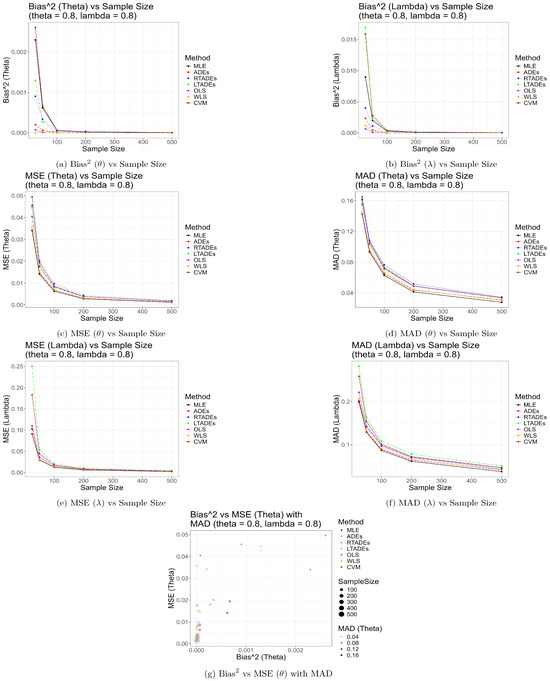
Figure 2. Graphical representation of simulation results for $\theta =0.8$, $\lambda =0.8$.

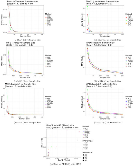
Figure 3. Graphical representation of simulation results for $\theta =1.5$, $\lambda =3.0$.

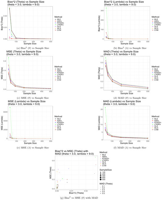
Figure 4. Graphical representation of simulation results for $\theta =3.0$, $\lambda =9.0$.

6. Illustration with Real Data

To evaluate the proposed SUEHL distribution, we analyzed two real datasets with distinct characteristics. The first, from Smith and Naylor [37], consists of fiber strength measurements, exhibiting asymmetric and skewed patterns ideal for testing lifetime distributions. The second, from Dasgupta [45], includes 50 observations of burr measurements with a 9 mm hole diameter and 2 mm sheet thickness, providing a manufacturing context to assess model flexibility. To provide insight into the structures of the datasets, we report their descriptive statistics in Table 5. The fiber strength dataset, scaled by 1/10 to fit the unit interval (0,1), has a mean of 0.151 and a median of 0.159, indicating slight right-skewness. The burr dataset, with a mean of 0.152 and a median of 0.160, shows moderate skewness and higher variability (standard deviation of 0.078), suitable for manufacturing applications. The parameters of the models were estimated using MLE in R (version 4.4.3) [41,42]. For the fiber dataset, the SUEHL estimates are $\theta =5.529,\lambda =6493.272$ ($-2logL=-260.72$), and for the burr dataset, $\theta =1.916,\lambda =8.324$ ($-2logL=-115.23$). We compared SUEHL against the beta, UEHL, Topp–Leone, and sine-G distributions using goodness-of-fit metrics: negative twice log-likelihood ($-2logL$), Akaike Information Criterion (AIC), Bayesian Information Criterion (BIC), Kolmogorov–Smirnov (KS), Anderson–Darling (AD), and Cramér–von Mises (CVM) statistics, with their p-values. These distributions were selected as they are bounded-domain models suitable for unit-interval data, aligning with the SUEHL’s focus on asymmetric reliability engineering applications. Table 6 and Table 7 summarize the results. For the fiber dataset, SUEHL yields the lowest $-2logL$ ($-260.72$), AIC ($-256.72$), BIC ($-252.44$), KS (0.15, $p=0.13$), AD (1.14, $p=0.29$), and CVM (0.20, $p=0.27$). For the burr dataset, it achieves $-2logL=-115.23$, AIC ($-111.23$), BIC ($-107.41$), KS (0.16, $p=0.15$), AD (1.23, $p=0.26$), and CVM (0.19, $p=0.28$). The beta and UEHL distributions are competitive but consistently outperformed, while Topp–Leone and sine-G show poor fits with high test statistics. To visually complement these results, Figure 5 illustrates the empirical cumulative distribution functions (ECDFs) of the datasets alongside the fitted SUEHL CDF, with the fiber strength dataset shown in the left graph and the burr dataset in the right graph, demonstrating the model’s strong alignment with both datasets.

Table 5. Descriptive statistics of the fiber strength and burr datasets.

Dataset	Mean	Median	Std. Dev.	Min	Max
Fiber Strength	0.151	0.159	0.032	0.055	0.224
Burr	0.152	0.160	0.078	0.020	0.320

Table 6. Goodness-of-fit results for fiber strength dataset.

Distribution	Parameters	$-2log\mathit{L}$	AIC	BIC	KS Stat	p (KS)	AD Stat	p (AD)	CVM Stat	p (CVM)
SUEHL	$\theta =5.529,\lambda =6493.272$	−260.72	−256.72	−252.44	0.15	0.13	1.14	0.29	0.20	0.27
Beta	$\theta =15.362,\lambda =86.681$	−244.43	−240.43	−236.14	0.21	0.01	2.89	0.03	0.53	0.03
UEHL	$\theta =5.781,\lambda =18030.733$	−259.71	−255.71	−251.43	0.15	0.11	1.24	0.25	0.21	0.24
Topp–Leone	$\theta =0.753$	−76.76	−74.76	−72.61	0.48	0.00	18.42	0.00	3.86	0.00
Sine-G	$\theta =1.561$	−52.42	−50.42	−48.27	0.68	0.00	37.40	0.00	8.26	0.00

Table 7. Goodness-of-fit results for burr dataset.

Distribution	Parameters	$-2log\mathit{L}$	AIC	BIC	KS Stat	p (KS)	AD Stat	p (AD)	CVM Stat	p (CVM)
SUEHL	$\theta =1.916,\lambda =8.324$	−115.23	−111.23	−107.41	0.16	0.15	1.23	0.26	0.19	0.28
Beta	$\theta =2.400,\lambda =13.524$	−111.86	−107.86	−104.04	0.20	0.04	1.56	0.16	0.29	0.15
UEHL	$\theta =2.001,\lambda =17.157$	−114.64	−110.64	−106.82	0.17	0.11	1.32	0.23	0.21	0.24
Topp–Leone	$\theta =0.700$	−65.29	−63.29	−61.38	0.33	0.00	6.73	0.00	1.25	0.00
Sine-G	$\theta =1.561$	−40.90	−38.90	−36.99	0.56	0.00	23.19	0.00	5.10	0.00

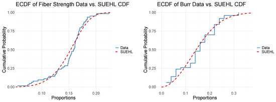
Figure 5. Empirical CDFs of the datasets compared to the fitted SUEHL CDF, with the fiber strength dataset shown in the left graph and the burr dataset in the right graph.

These results underscore versatility of the SUEHL distribution for applications in reliability engineering and manufacturing, offering a robust two-parameter model that handles diverse, skewed datasets.

7. Conclusions

The SUEHL distribution represents a significant advancement in statistical distribution theory, addressing the need for flexible models to capture intricate patterns in modern datasets. By integrating the UEHL distribution with the sine-G family, this study introduces a versatile two-parameter model capable of accommodating diverse data shapes within the unit interval. Key findings include the comprehensive derivation of statistical properties, such as quantiles, moments, stress–strength reliability, inverse hazard rate, and mean residual life, which enhance the SUEHL’s applicability in reliability engineering. Simulation studies demonstrate the efficacy of various estimation techniques. Real data applications, compared with unit-interval distributions, confirm the SUEHL’s superior fit for the datasets, offering practical implications for decision-making in reliability engineering and manufacturing. The SUEHL’s advantages include its flexible density shapes and robust reliability measures, though its computational complexity may pose challenges for large datasets. Future studies could explore multivariate extensions of the SUEHL to model joint reliability, potentially advancing statistical analysis further. These contributions fill a critical gap in modeling asymmetric unit-interval data, providing a powerful tool for real-world applications.

References

- Eugene, N.; Lee, C.; Famoye, F. Beta-normal distribution and its applications. Commun. Stat. Theory Methods 2002, 31, 497–512. [Google Scholar] [CrossRef]
- Alzaatreh, A.; Famoye, F.; Lee, C. A new method for generating families of continuous distributions. Metron 2013, 71, 63–79. [Google Scholar] [CrossRef]
- Marshall, A.; Olkin, I. A new method for adding a parameter to a family of distributions with applications to the exponential and Weibull families. Biometrika 1997, 84, 641–652. [Google Scholar] [CrossRef]
- Yegen, D.; Ozel, G. Marshall-Olkin half logistic distribution with theory and applications. Alphanumeric J. 2018, 6, 408–416. [Google Scholar] [CrossRef]
- Elgarhy, M.; Hassan, A.S.; Fayomi, S. Maximum likelihood and Bayesian estimation for two-parameter type I half logistic Lindley distribution. J. Comput. Theor. Nanosci. 2018, 15, 1–9. [Google Scholar] [CrossRef]
- Al-Shomrani, A.; Arif, O.; Shawky, A.; Hanif, S.; Shahbaz, M.Q. Topp-Leone family of distributions: Some properties and application. Pak. J. Stat. Oper. Res. 2016, 12, 443–451. [Google Scholar] [CrossRef]
- Hassan, A.S.; El-Sherpieny, E.A.; El-Taweel, S.A. New Topp Leone-G family with mathematical properties and applications. J. Phys. Conf. Ser. 2021, 1860, 012011. [Google Scholar] [CrossRef]
- Hassan, A.S.; Elgarhy, M.; Haq, M.A.; Alrajhi, S. On type II half logistic Weibull distribution with applications. Math. Theory Model. 2019, 19, 49–63. [Google Scholar] [CrossRef]
- Mohammad, G.S. A new two-parameter modified half-logistic distribution: Properties and Applications. Stat. Optim. Inf. Comput. 2022, 10, 589–605. [Google Scholar] [CrossRef]
- Kumar, D.; Singh, U.; Singh, S.K. A new distribution using sine function-its application to bladder cancer patients data. J. Stat. Appl. Prob. 2015, 4, 417–427. [Google Scholar]
- Cordeiro, G.M.; Alizadeh, M.; Ortega, E.M.M. The exponentiated half logistic family of distributions: Properties and applications. J. Probab. Stat. 2014, 2014, 864396. [Google Scholar] [CrossRef]
- Mahmood, Z.; Chesneau, C.; Tahir, M.H. A new sine-G family of distributions: Properties and applications. Bull. Comput. Appl. Math. 2019, 7, 53–81. [Google Scholar]
- Hassan, A.S.; Alsadat, N.; Elgarhy, M.; Sapkota, L.P.; Balogun, O.S.; Gemeay, A.M. A novel asymmetric form of the power half-logistic distribution with statistical inference and real data analysis. Electron. Res. Arch. 2025, 33, 791–825. [Google Scholar] [CrossRef]
- Muhammad, M.; Alshanbari, H.M.; Alanzi, A.R.A.; Liu, L.; Sami, W.; Chesneau, C.; Jamal, F. A new generator of probability models: The exponentiated sine-G family for lifetime studies. Entropy 2021, 23, 1394. [Google Scholar] [CrossRef]
- Jose, J.K.; Manoharan, M. Beta half logistic distribution: A new probability model for lifetime data. J. Stat. Manag. Syst. 2016, 19, 587–604. [Google Scholar] [CrossRef]
- Bantan, R.; Hassan, A.S.; Elsehetry, M.; Kibria, B.M. Half-logistic xgamma distribution: Properties and estimation under censored samples. Discrete Dyn. Nat. Soc. 2020, 2020, 9136513. [Google Scholar] [CrossRef]
- Hassan, A.S.; Fayomi, A.; Algarni, A.; Almetwally, E.M. Bayesian and non-Bayesian inference for unit-exponentiated half-logistic distribution with data analysis. Appl. Sci. 2022, 12, 11253. [Google Scholar] [CrossRef]
- Özbilen, Ö.; Genç, A.I. A bivariate extension of the omega distribution for two-dimensional proportional data. Math. Slovaca 2022, 72, 1605–1622. [Google Scholar] [CrossRef]
- Usman, R.M.; Haq, A.M.; Talib, J. Kumaraswamy half-logistic distribution: Properties and applications. J. Stat. Appl. Prob. 2017, 6, 597–609. [Google Scholar] [CrossRef]
- Anwar, M.; Bibi, A. The half-logistic generalized Weibull distribution. J. Probab. Stat. 2018, 2018, 8767826. [Google Scholar] [CrossRef]
- Algarni, A.; Almarashi, A.M.; Elbatal, I.; Hassan, A.S.; Almetwally, E.M.; Daghistani, A.M.; Elgarhy, M. Type I half logistic Burr X-G family: Properties, Bayesian, and non-Bayesian estimation under censored samples and applications to COVID-19 data. Math. Probl. Eng. 2021, 2021, 5461130. [Google Scholar] [CrossRef]
- Hashempour, M. An extended type I half-logistic family of distributions: Properties, applications and different method of estimations. Math. Slovaca 2022, 72, 745–764. [Google Scholar] [CrossRef]
- Arshad, R.M.I.; Tahir, M.H.; Chesneau, C.; Khan, S.; Jamal, F. The gamma power half-logistic distribution: Theory and applications. Sao Paulo J. Math. Sci. 2023, 17, 1142–1169. [Google Scholar] [CrossRef]
- Alghamdi, S.M.; Shrahili, M.; Hassan, A.S.; Gemeay, A.M.; Elbatal, I.; Elgarhy, M. Statistical inference of the half logistic modified Kies exponential model with modeling to engineering data. Symmetry 2023, 15, 586. [Google Scholar] [CrossRef]
- Alizadeh, M.; MirMostafee, S.; Ortega, E.; Ramires, T.; Cordeiro, G. The odd log-logistic logarithmic generated family of distributions with applications in different areas. J. Stat. Distrib. App. 2017, 4, 1–25. [Google Scholar] [CrossRef][Green Version]
- Nadarajah, S.; Kotz, S. The exponentiated Fréchet distribution. Interstat 2003, 14, 1–7. [Google Scholar]
- Oliveira, J.; Santos, C.; Xavier, D.; Trindade, D.; Cordeiro, G.M. The McDonald half-logistic distribution: Theory and practice. Commun. Stat. Theory Methods 2016, 45, 2005–2022. [Google Scholar] [CrossRef]
- Xavier, T.; Jose, J.K. A study of stress-strength reliability using a generalization of power transformed half-logistic distribution. Commun. Stat. Theory Methods 2020, 50, 4335–4351. [Google Scholar] [CrossRef]
- Nadarajah, S.; Cordeiro, G.M.; Ortega, E.M.M. General results for the Kumaraswamy-G distribution. J. Stat. Comput. Simul. 2013, 83, 951–979. [Google Scholar] [CrossRef]
- Xavier, T.; Jose, J.K.; Nadarajah, S. An additive power-transformed half-logistic model and its applications in reliability. Qual. Reliab. Eng. Int. 2022, 38, 3179–3196. [Google Scholar] [CrossRef]
- Hjorth, U. A reliability distribution with increasing, decreasing, constant and bathtub-shaped failure rates. Technometrics 1980, 22, 99–107. [Google Scholar] [CrossRef]
- Mudholkar, G.S.; Srivastava, D.K. Exponentiated Weibull family for analyzing bathtub failure-rate data. IEEE Trans. Reliab. 1993, 42, 299–302. [Google Scholar] [CrossRef]
- Lemonte, A.J.; Cordeiro, G.M.; Ortega, M.M.E. On the additive Weibull distribution. Commun. Stat. Theory Methods 2014, 43, 2066–2080. [Google Scholar] [CrossRef]
- Xie, M.; Lai, C.D. Reliability analysis using an additive Weibull model with bathtub-shaped failure rate function. Reliab. Eng. Syst. Saf. 1995, 52, 87–93. [Google Scholar] [CrossRef]
- Wang, F.K. A new model with bathtub-shaped failure rate using an additive Burr XII distribution. Reliab. Eng. Syst. Saf. 2000, 70, 305–312. [Google Scholar] [CrossRef]
- Hassan, A.H.; Elgarhy, M.; Shakil, M. Type II half logistic family of distributions with applications. Pak. J. Stat. Oper. Res. 2017, 13, 245–264. [Google Scholar] [CrossRef]
- Smith, R.L.; Naylor, J.C. A comparison of maximum likelihood and Bayesian estimators for the three-parameter Weibull distribution. Appl. Stat. 2002, 36, 358–369. [Google Scholar] [CrossRef]
- Cheng, R.C.H.; Amin, N.A.K. Maximum product-of-spacings estimation with applications to the log-normal distribution. Univ. Wales IST Math Rep. 1979, 79, 103. [Google Scholar]
- Cheng, R.C.H.; Amin, N.A.K. Estimating parameters in continuous univariate distributions with a shifted origin. J. R. Stat. Soc. Ser. B Methodol. 1983, 45, 394–403. [Google Scholar] [CrossRef]
- Ranneby, B. The maximum spacing method: An estimation method related to the maximum likelihood method. Scand. J. Stat. 1984, 11, 93–112. [Google Scholar]
- Henningsen, A.; Toomet, O. maxLik: A package for maximum likelihood estimation in R. Comput. Stat. 2011, 26, 443–458. [Google Scholar] [CrossRef]
- R Core Team. R: A Language and Environment for Statistical Computing; Foundation for Statistical Computing: Vienna, Austria, 2013. [Google Scholar]
- Aarset, M.V. How to identify a bathtub hazard rate. IEEE Trans. Reliab. 1987, 36, 106–108. [Google Scholar] [CrossRef]
- Krishnarani, S.D. On a power transformation of half-logistic distribution. J. Probab. Stat. 2016, 2016, 1–10. [Google Scholar] [CrossRef]
- Dasgupta, R. On the distribution of burr with applications. Sankhya B 2011, 73, 1–19. [Google Scholar] [CrossRef]
Disclaimer/Publisher’s Note: The statements, opinions and data contained in all publications are solely those of the individual author(s) and contributor(s) and not of MDPI and/or the editor(s). MDPI and/or the editor(s) disclaim responsibility for any injury to people or property resulting from any ideas, methods, instructions or products referred to in the content. |
© 2025 by the authors. Licensee MDPI, Basel, Switzerland. This article is an open access article distributed under the terms and conditions of the Creative Commons Attribution (CC BY) license (https://creativecommons.org/licenses/by/4.0/).