Abstract
Determining the position values of the effectors in a robot to enable its end effector to perform a specific task is a recurrent challenge in robotics. Diverse methodologies have been explored to address this problem, each with distinct advantages and limitations. This work proposes a metaheuristic-based approach to solve a sequence of optimization problems associated with the discretized trajectory of the end effector. Additionally, a method to identify a functional model that describes the effector trajectories is introduced using the same optimization technique. The key contribution lies in algorithmic adjustments that enhance the metaheuristic solutions by leveraging the behavior of the robot and the influence of the tracking task on the search space. Specifically, two operations are modified in the initialization process of the candidate solution. The proposed biased initialization with variable weights improves positional accuracy (72.5%) in relation to methods without dynamic updates. Additionally, the standard deviation was reduced by (89%). For industrial implementations, modern controllers can directly encode effector positions via parametric functions. The results of this proposal formulate optimization problems whose solutions yield the parameters of a time-dependent mathematical model describing the movement of the effector.
Keywords:
optimization; metaheuristic algorithm; inverse kinematics problem; kinematic chain; identification technique MSC:
65k10
1. Introduction
A robot is a multifunctional reprogrammable manipulator designed to move parts, tools, or devices through previously scheduled movements [1]. Industrial robots serve as labor in different processes. The possible tasks for which they can be programmed include those that correspond to automated routines that are repeated continuously; for example, welding, painting, and assembly, among others [2,3,4]. To program these routines in robot controllers, it is necessary to solve the inverse kinematics problem (IKP), which consists of finding the angular orientation of the joints since the Cartesian coordinates of the final effector are already determined by the trajectory defined to perform a given task.
Different methodologies have been developed in diverse works to address the problem of inverse kinematics in robots, such as the analytical approach in [5,6,7], where using a geometric analysis, a mathematical model is obtained for solving the problem. The main difficulty with this approach is that obtaining the model is a complicated task that requires more complex analysis compared to others that use numerical techniques. Additionally, there may be points of singularity depending on the imposed constraints in which, given a desired position, multiple solutions (postures) generate undesired behaviors when implementing the solution in a controller. The alternatives to address these cases involve complex analysis of the model itself and the implementation of strategies to create trajectories that evade these points while also ensuring that the robot fulfills its task, as shown in [8].
Other approaches to address the problem of inverse kinematics are based on intelligent computing techniques. Although they share a general technique, the approaches can vary, as documented in [9,10], in which different methods are presented, from collaborative networks to linking the direct kinematic model with the architecture of the neural network itself to produce a modular system. On the other hand, using optimization techniques to minimize an error function that links the mathematical description of the desired posture and its associated angular values is another approach that has gained followers in recent years due to the simplicity of the optimization algorithms [11,12,13,14].
Although this last approach lacks the response speed of analytical methods, it has the advantage that when searching in the configuration space of direct kinematics, the results can be easily exported to industrial point-to-point trajectory programming controllers since singularities such as division by 0 in analytical parametrization are not presented. In addition, these algorithms do not depend on a training dataset.
The advantage of avoiding singularities or that the search algorithm will always return a single solution that can be bounded given a series of constraints in the optimization model is of special interest for this work, since this allows for almost direct implementation of the result as a routine in a serial robot. There are several types of singularities that cause loss of control, high speeds, or unpredictable behavior.
In this work, a methodology is presented to obtain a parametric solution for the IKP in the tasks of tracking a closed path based on minimizing an objective function that quantifies the error between the ideal trajectory and the real one found by a metaheuristic algorithm. A fanuc 200 series robot was used as a case study, and it was solved by applying differential evolution (DE). Following the methodology for solving the IKP, it is possible to avoid the singularity of the robotic wrist by generating a trajectory described only by the joint angular values. This is an important contribution not only in the field of robotics but also in the field of metaheuristic methods since it represents an alternative way to avoid problems associated with this type of robot [15].
As an additional characteristic using the resulting values, DE was also implemented to identify a functional model for the movement of the joints along a closed trajectory. This aspect is especially useful for maintaining compatibility with other robot controllers with similar architectures. Furthermore, for practical purposes, it is not convenient to address a high number of discrete points since it is an inefficient use of memory and produces problems such as loss of motion smoothness. The functional representation can be useful for more complex analyses in relation to the task and the limits of the controller.
In summary, the contributions of this work are as follows:
- The formulation of an optimization problem whose solution represents the position values for inverse kinematics in a 6-DOF serial robot.
- The determination of a mathematical function model for closed paths.
- The proposal and incorporation of an adaptive operator that biases populations in the DE algorithm to achieve the conditions for angular movements in a closed trajectory that coincide with a periodic function.
This paper is organized as follows: Section 2 describes the forward kinematics (FKs) as the search space for DE, the general metaheuristic function and its modifications, and the applied methodology. Section 3 presents the experiments conducted, their results, and the corresponding discussion. Section 4 includes conclusions and future work.
2. Materials and Methods
This section presents the mathematical model of direct kinematics, the optimization approach for the IKP, the metaheuristic technique, the identification process, and the final methodology for the complete process.
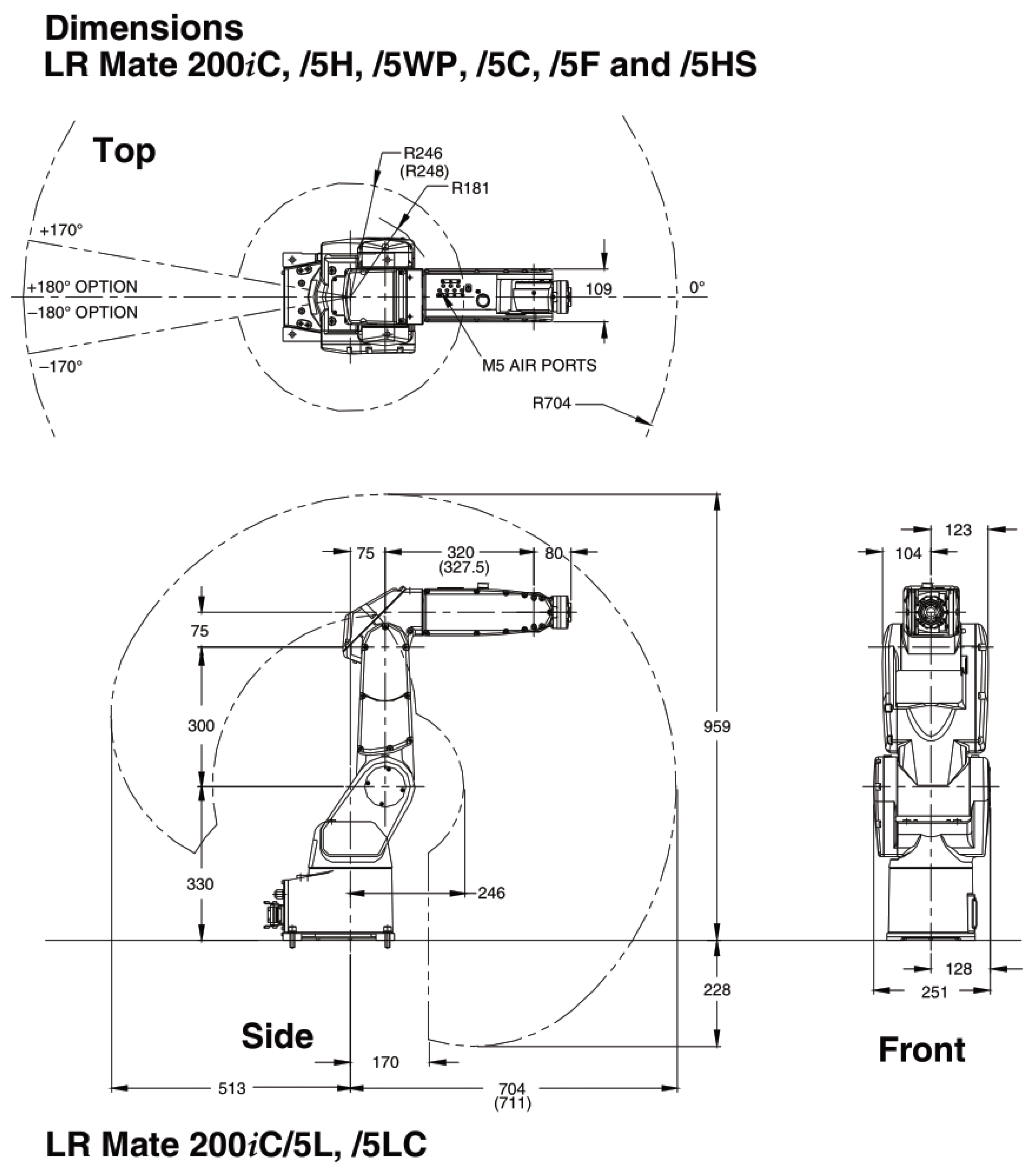
As shown in different works [14,16,17], to search for solutions referring to the IKP, it is possible to start from the model referred to as the FK of the robot. To achieve this, different approaches have involved a series of homogeneous transformations. In this work, the convention [15] was selected to model the FK of the 200 series robot as the case study; see Figure 1.
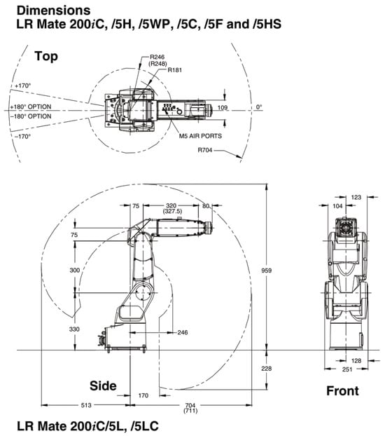
Figure 1.
Fanuc m-200 model [18].
According to the description of the homogeneous transformation matrix in [15,19], the column vector denoted by in the expression (1) represents the desired position of the effector. This matrix is the result of the transformation matrices described by (2) and whose i parameters are found in Table 1.

Table 1.
Parameters for homogeneous transformations.
2.1. Optimization Approach
An optimization problem is defined mathematically as a cost function that is to be maximized or minimized, whose candidate solutions are bounded by the search space and may or may not contain inequality and equality restrictions, as shown in Equations (3)–(5).
subject to:
For the case study, the solution vector can be changed by the vector that represents the angular values of the robot’s effectors. The function f becomes an error function () that uses FK and a desired point (); this function is described below (6):
The methods for solving this type of problem are varied, and one of them is the use of metaheuristics that have been useful for different engineering problems [20,21,22]. Some of the metaheuristics applied to solve the IKP are the particle optimization algorithm, artificial bee colony, and differential evolution, among others [12,23]. The selection of the algorithm is usually subject to particular objectives such as improving the search for the global optimum, fast response, and flexibility to implementing operators, among others. For this work, it has been decided to use the differential evolution algorithm since it has proven to be efficient for solving and obtaining the inverse kinematics given a trajectory discretized by points [14].
2.2. Differential Evolution Algorithm
The differential evolution algorithm is an algorithm that is based on a set of solutions called a population. It is used to find global optima. It was introduced by Storn and Price, and it is inspired by biological concepts of evolution to establish its operators that update the population [24].
The general structure consists of the initialization of a population of individuals or candidate solutions that are updated iteratively according to the crossover, mutation, and selection operators until a stopping criterion is met.
The mutation operation consists of generating a mutant vector for each individual in the population. This operation has different forms, but for this work, the rand/1/bin version is used. Its formula for generating the mutant vector is denoted by (7), where the vectors are randomly selected and different from each other, while F is called the mutation factor.
Once the mutant vector is obtained, the cross between the characteristics of the objective vector and the result of the mutation is performed. In the version used, the binary cross is used, the process of which is denoted by (8), where CR defines the crossover factor. Each element j of the cross-vector is selected according to the random values and the selection rule.
Finally, a selection is made between the vector of the previous generation in the population and the one obtained by the mutation and crossover operations in such a way that the one with the best performance in the objective function will be kept in the next iteration while the other will be discarded.
2.3. DE Considerations for the Case Study
The initialization stage of the algorithm is not usually discussed in most works because in order to find the optimum, the entire space is explored; the individuals are initialized randomly, taking as limits the upper and lower bounds of the search space. Another reason for this is that at least one solution with performance close to the optimum is not usually known, but in the case of manipulator robots, it is expected that they do not make an abrupt change with respect to their current posture when following a trajectory, which is why the biased initialization exposed in [14] will be resumed, whose formula is described below (10):
The expression (10) is interpreted as a bias in the initialization in which the set of individuals in the population represent a set of robot postures with a degree of similarity regulated by M. The index implies that for a trajectory, the best solution of the previous point represents the best candidate at the beginning of the algorithm to find the new configuration k.
For closed paths in [14], a modification to this approximation was proposed in which an average is established with respect to the initial position to which the robot must return at the end of the route. The solution of the previous optimization problem was referred to as the IKP. That expression corresponds with (11). The use of this initialization reported good results in the cited work, but in the experiments carried out, it did not have a good performance at the most distant points of the trajectory with respect to the initial posture. This motivated us to propose a second model that will dynamically balance the contribution of each one of the parts (initial posture and best previous solution). The resulting expression is given in (12). This approach is used to prioritize the previous solutions at the ends of the trajectory, and as it finishes its journey, re-prioritize the initial posture. The value d is the euclidean distance between the initial point of the path and some , and refers to the distance from the farthest point in the path.
It is important to notice that this approach biases the search and maintains a degree of similarity in its posture throughout the executions; if another pose is required for the same path tracking, it is necessary to pre-position the robot. For cases where the position cannot be maintained strictly, the algorithm will search for the solution with the lowest penalty in the objective function.
2.4. Bias Operators, Differential Evolution, and Singularities
The DE algorithm was chosen due to the low number of parameters required to tune it, as well as its compatibility with the proposed operators. One limitation of these operators is that they are not suitable for all metaheuristics. In the artificial bee colony algorithm [25], there is an operator that restarts the solutions after a certain period in which the solution does not improve (abandonment of food source). The above opposes the characteristic that is exploited in this work, which consists of using prior information. The search is biased in order to converge to a nearby solution while maintaining some degree of similarity between the postures adopted by the robot along the trajectory. Repulsion strategies to avoid local convergence in various metaheuristic techniques would nullify the advantage of the proposed operator and could generate a solution with a smaller error but with a greater displacement from the previous posture, which would produce undesirable behavior.
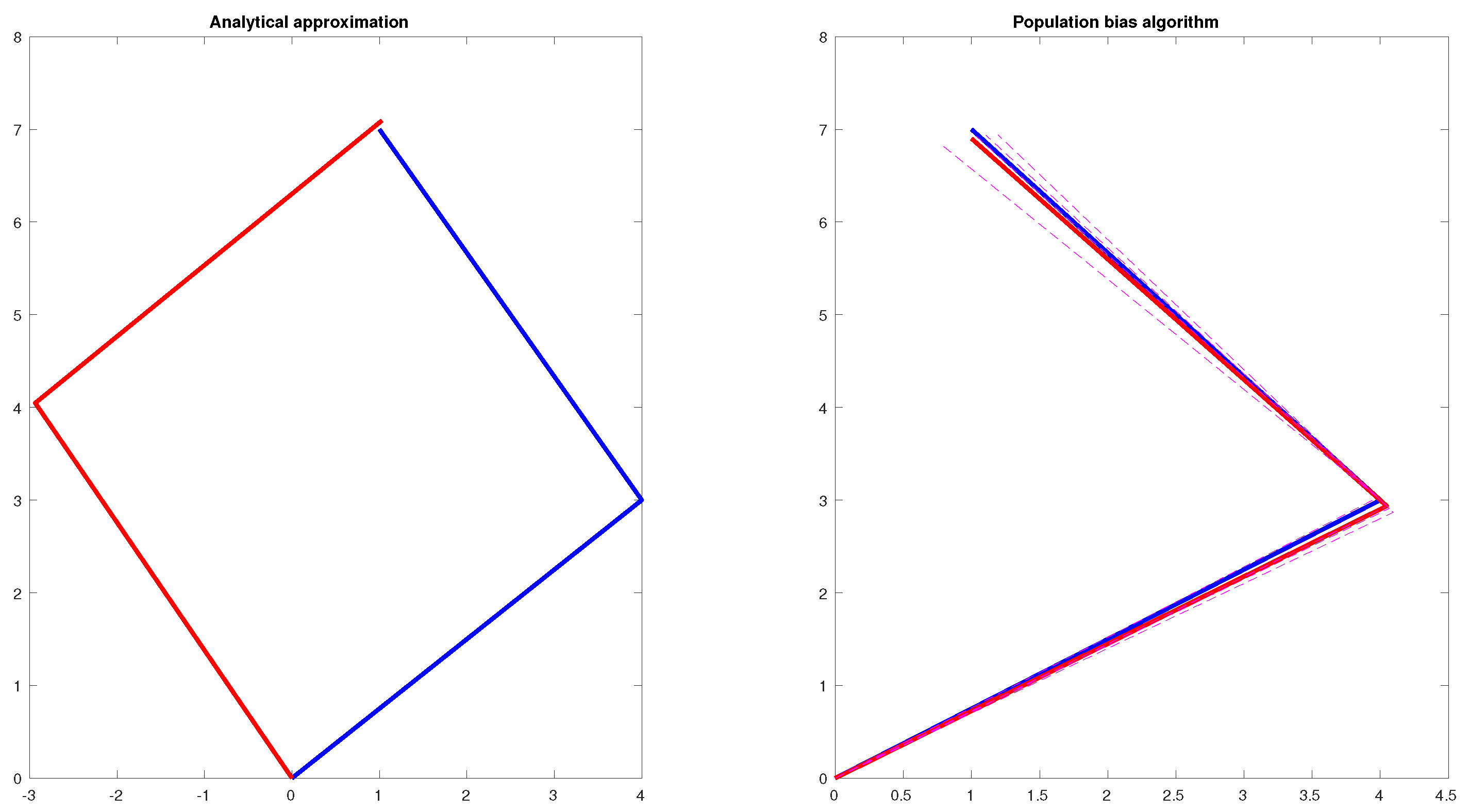
The bias in the candidate solutions increases the probability of finding solutions that have similar values to the previous stance in the sequence of optimization problems, which limits the generation of movement sequences with abrupt changes or that restrict movement due to the emergence of multiple solutions. For example, in the geometric approach described by Equations (13)–(15), where x and y are the coordinates in space, and are the lengths of the links, and and are the values of the effectors, it is necessary to analyze the subspaces between pairs of links to detect when the inverse trigonometric functions associated with the inverse kinematic model could result in an abrupt change.
Figure 2 shows a phenomenon in which, when implementing the inverse kinematics model for a pair of successive links without any additional adjustments, a change in elbow configuration occurs when moving from a position that maps to . In contrast, in the exploration based on error penalization and the direct kinematic model with population constraints in the metaheuristic, the candidate solutions converge to a solution similar to the previous posture, avoiding abrupt changes (singularities).
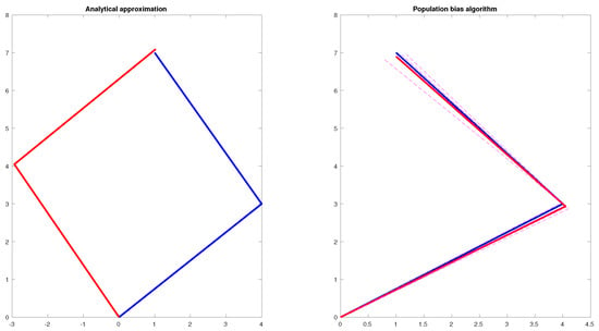
Figure 2.
On the left side, the analytical solutions for two nearby points are shown, indicating a change in orientation. On the right, the solutions for the same points are shown with the DE algorithm, with some candidate solutions highlighted in magenta to apply the bias.
In practice, when the controller detects a singularity given its programming, the robot stops, and to get it out of that point, it operates in direct mode (control over each joint) to move it to a different position. This is similar to the work done by the metaheuristic in which the operator seeks a solution solely by manipulating the values of the effectors. The results found can then be exported as a list of points to later be integrated as an executable program in direct mode in the robot’s controller, meaning that the method is not included in the controller; only its result is exported in point format or as the identified function for a specific trajectory.
2.5. Identification
Once the angular values of the robot along the path have been obtained, it would be convenient to have a mathematical model that describes its movement instead of just having the discrete data. In order to achieve this, it is proposed to use the differential evolution algorithm to perform parametric identification, taking advantage of the fact that thanks to the methodology for solving the IKP, the points constitute points of a periodic signal and therefore can be described as a Fourier series [26].
Considering form (16) and m terms, the problem is to find the terms and such that the function (17) is minimized, which represents an error function between the k samples mapped in (obtained by the resolution of IKP for the P points) and the values mapped at the same times by the truncated Fourier series representation (). For the optimization function, an error function that calculates the difference between the k points mapped by and the from the resolution of the IKP for the path, the vector contains the parameters .
It is possible to select a finite and computationally feasible number for identification, but it is suggested that it be not very high because in order to minimize the error, and given the number of points referring to the trajectory, it is possible that the algorithm finds solutions with abrupt changes in the part that does not contemplate information since it is not penalized in the proposed objective function.
2.6. Methodology Description
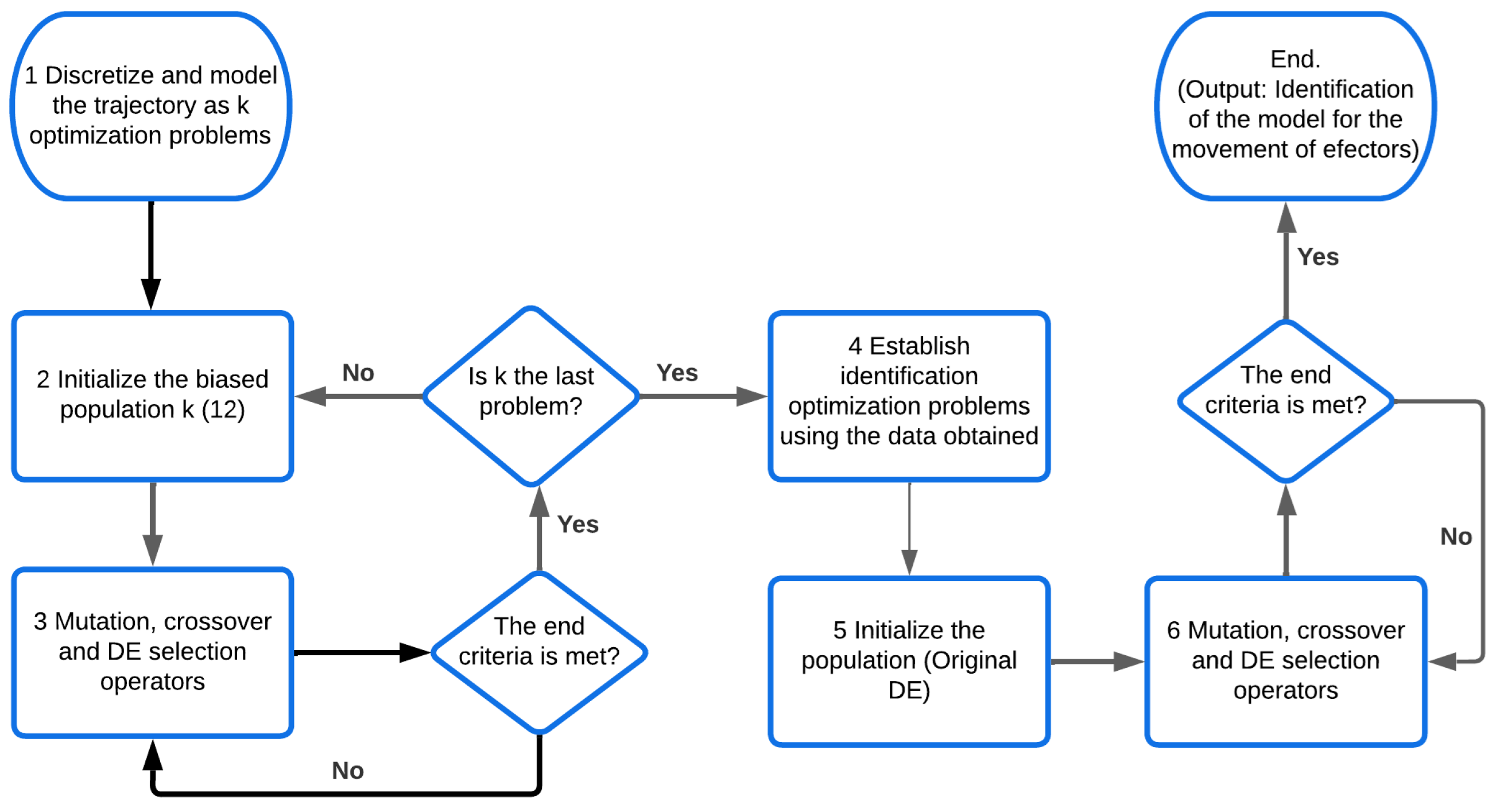
This section presents the steps to follow to replicate the experiments. The first step is to discretize the trajectory to be followed and model each point as an optimization problem, which must be solved in sequence.
As a second step, each of the optimization problems must be solved iteratively using the differential evolution algorithm with biased initialization, which uses as parameters the initial position of the trajectory and the solution to the previous optimization problem in the sequence described in step 1.
Finally, the solutions obtained will be used to construct the approximation of the continuous model for the motion of the effectors in order to pose a series of independent optimization problems whose solution represents the model identified by a truncation in the Fourier series. The entire methodology is shown in Figure 3.
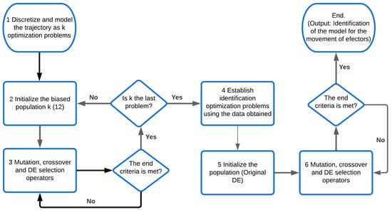
Figure 3.
Flowchart of the methodology.
3. Experiments and Results
In this section, the experiments carried out are described and their results are analyzed. Two experiments were carried out. In the first case, a sequence of optimization problems related to the points that make up a circular trajectory was established. In the resolution methodology in the metaheuristic part, each of the proposals is evaluated to bias the initialization of the population. Ten runs were performed with each approximation in order to compare the results since due to the random components of the DE, it is possible to have different results in each execution.
For the second experiment, the best performing approach was used to identify a functional model describing the trajectory of the effectors. The identification results are compared with the points obtained discretely in the first experiment.
Both experiments were performed using MATLAB R2020a software on a computational platform with the following specifications: Intel i7 processor @3.70 GHz, 16 GB RAM, and Windows 10 operating system. In addition, the tuning parameters for DE were selected according to the recommendations in [27,28], taking the following values: mutation factor , crossover probability , and number of individuals throughout all the generations.
3.1. First Experiment
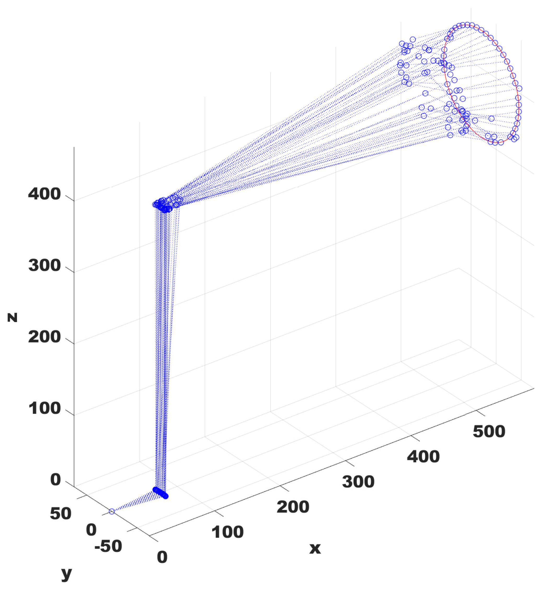
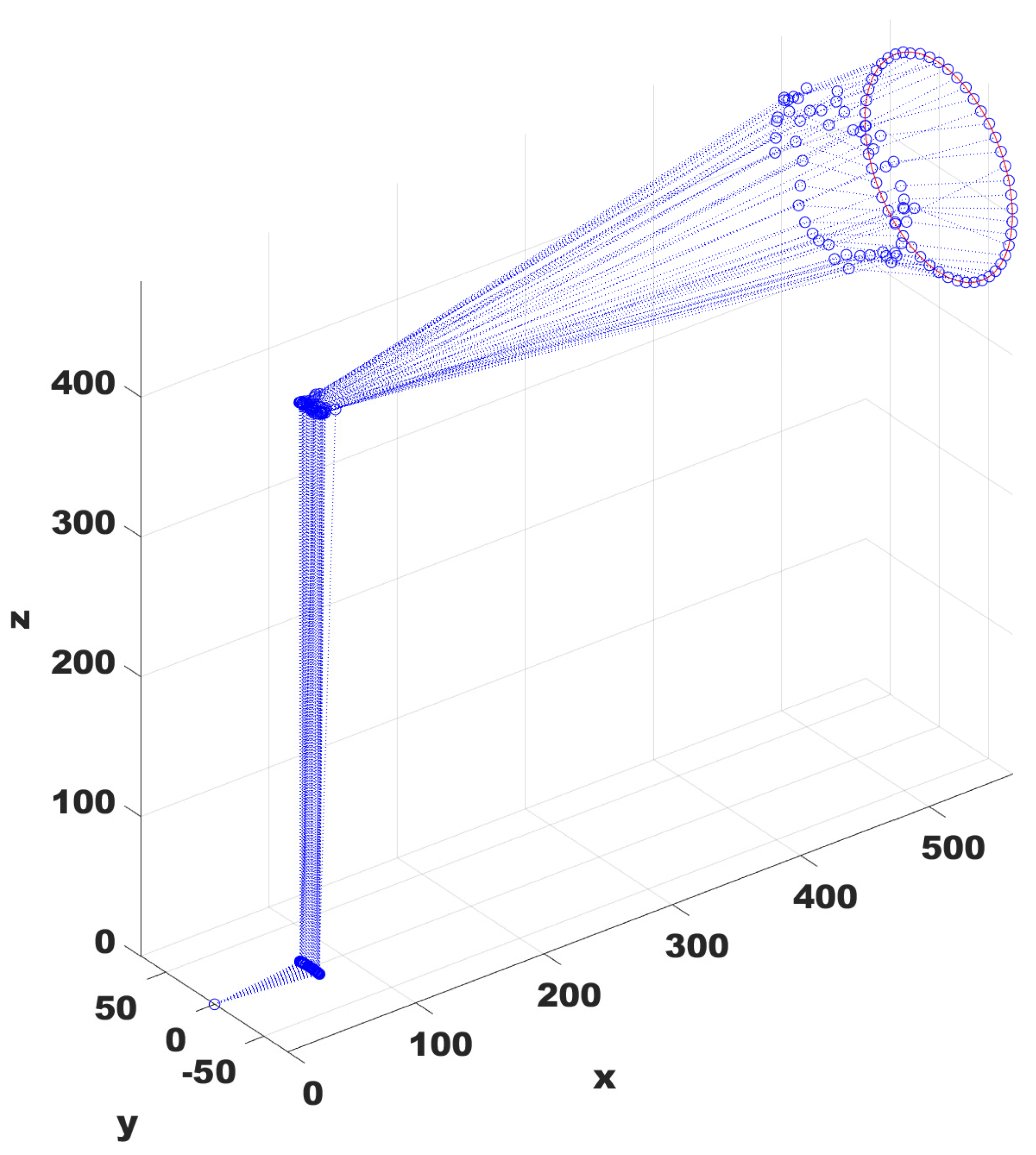
For the first experiment, a closed trajectory was designed, having as the first point the initial position of the robot given a randomly selected configuration. Each of the points on this trajectory represents an IKP by itself. These are solved sequentially using as the bias individual, which is the solution to the previous problem. In the case of the first problem, corresponds to the initial posture of the robot. For each optimization problem, the stop criteria were a limit of 100,000 evaluations of the objective function or to obtain a solution whose error function is lower than 0.001 = . Table 2 reports the results with the fixed and dynamic weighting described in Equations (11) and (12). Additionally, Figure 4 and Figure 5 show a representation of the robot’s links throughout a run.

Table 2.
Results of the first experiment.
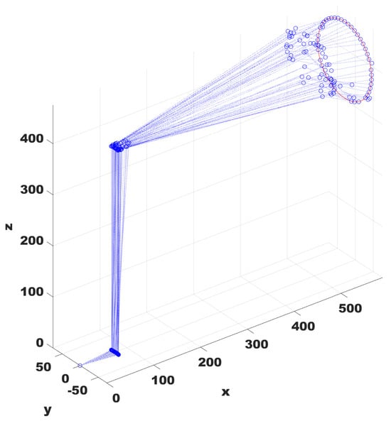
Figure 4.
Solutions for the optimization problems of the circular trajectory using the constant balance between the best solution and the initial posture.
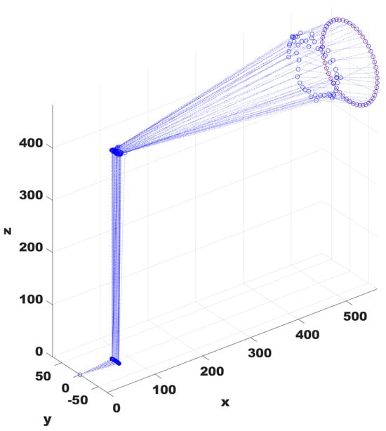
Figure 5.
Solutions for the optimization problems of the circular trajectory using the dynamic balance between the best solution and the initial posture.
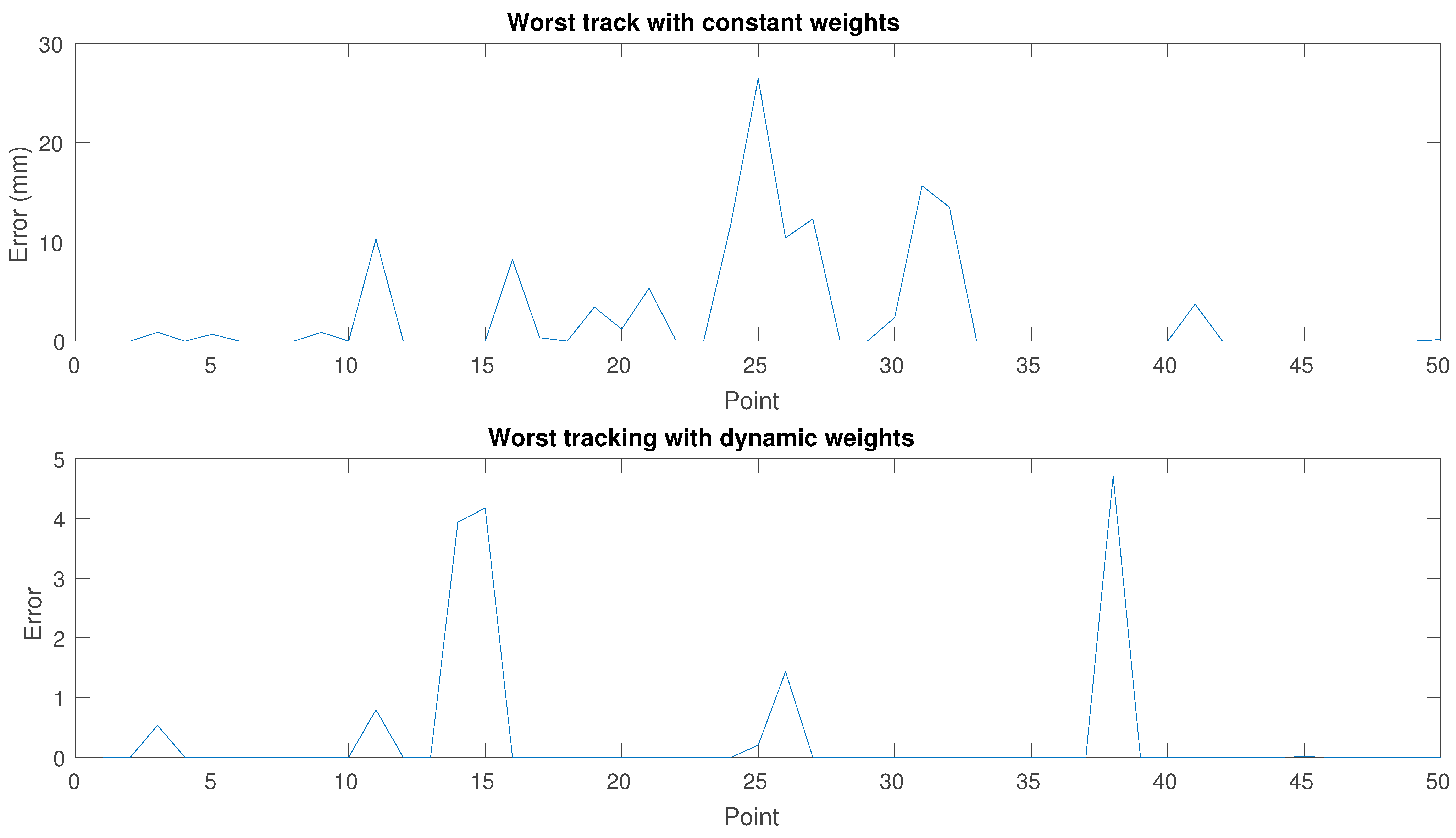
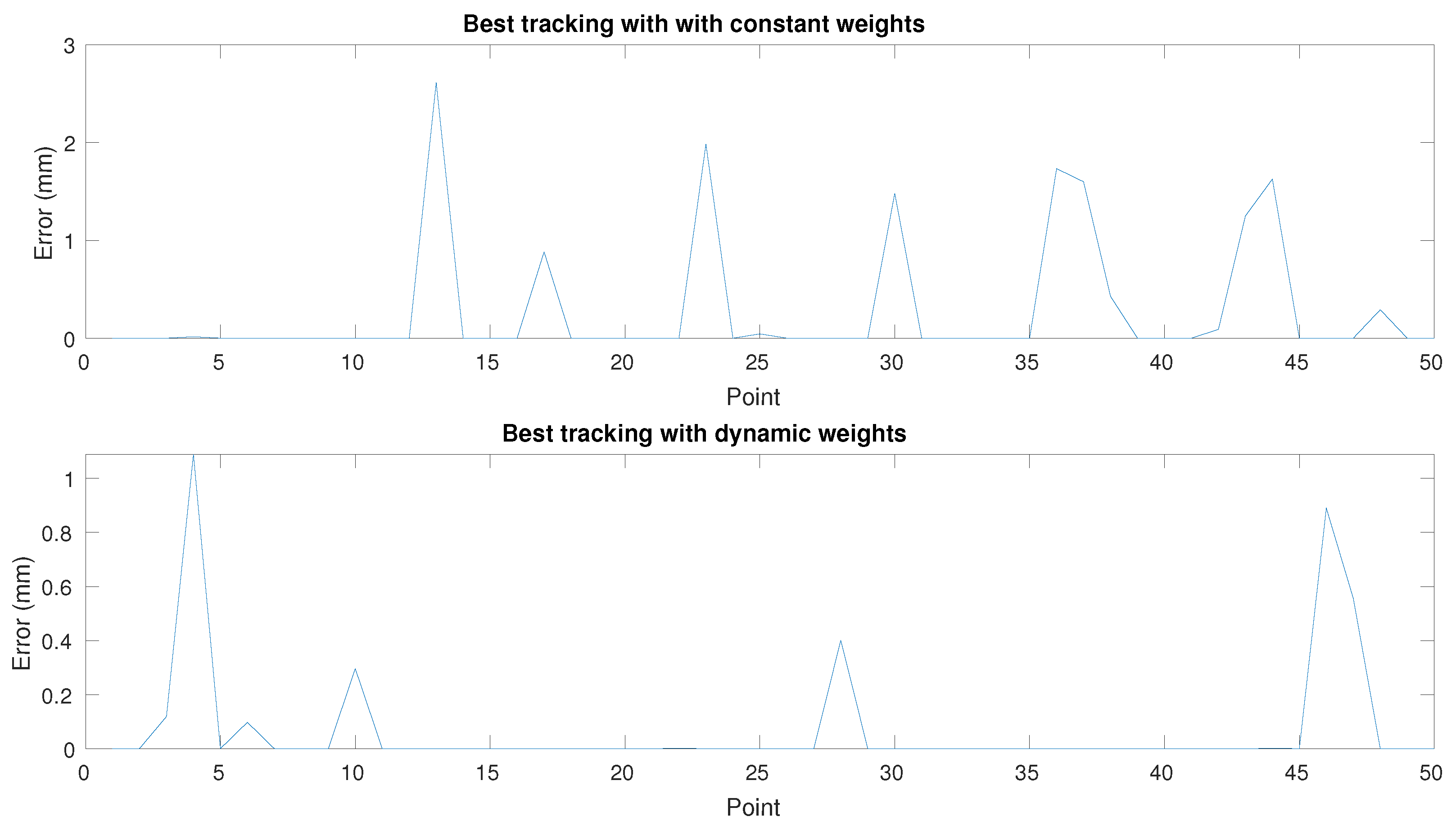
Figure 6 and Figure 7 report a comparison between the best and worst error functions along the path. Table 2 only shows the weighting of the sum of errors and does not provide additional information.
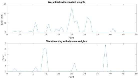
Figure 6.
Error function for each point in the worst runs for each approach (Run 5 for first approach and run 6 for second approach).
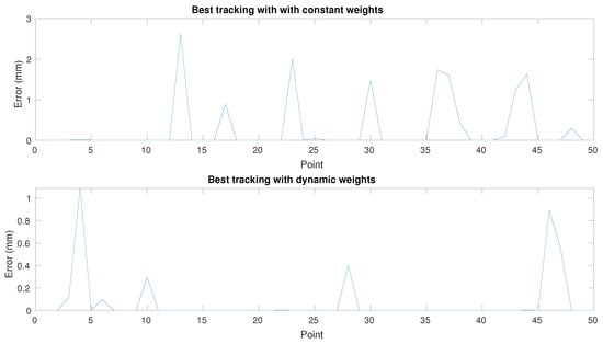
Figure 7.
Error function for each point in the best runs for each approach (run 10 for first approach and run 8 for second approach).
3.2. Second Experiment
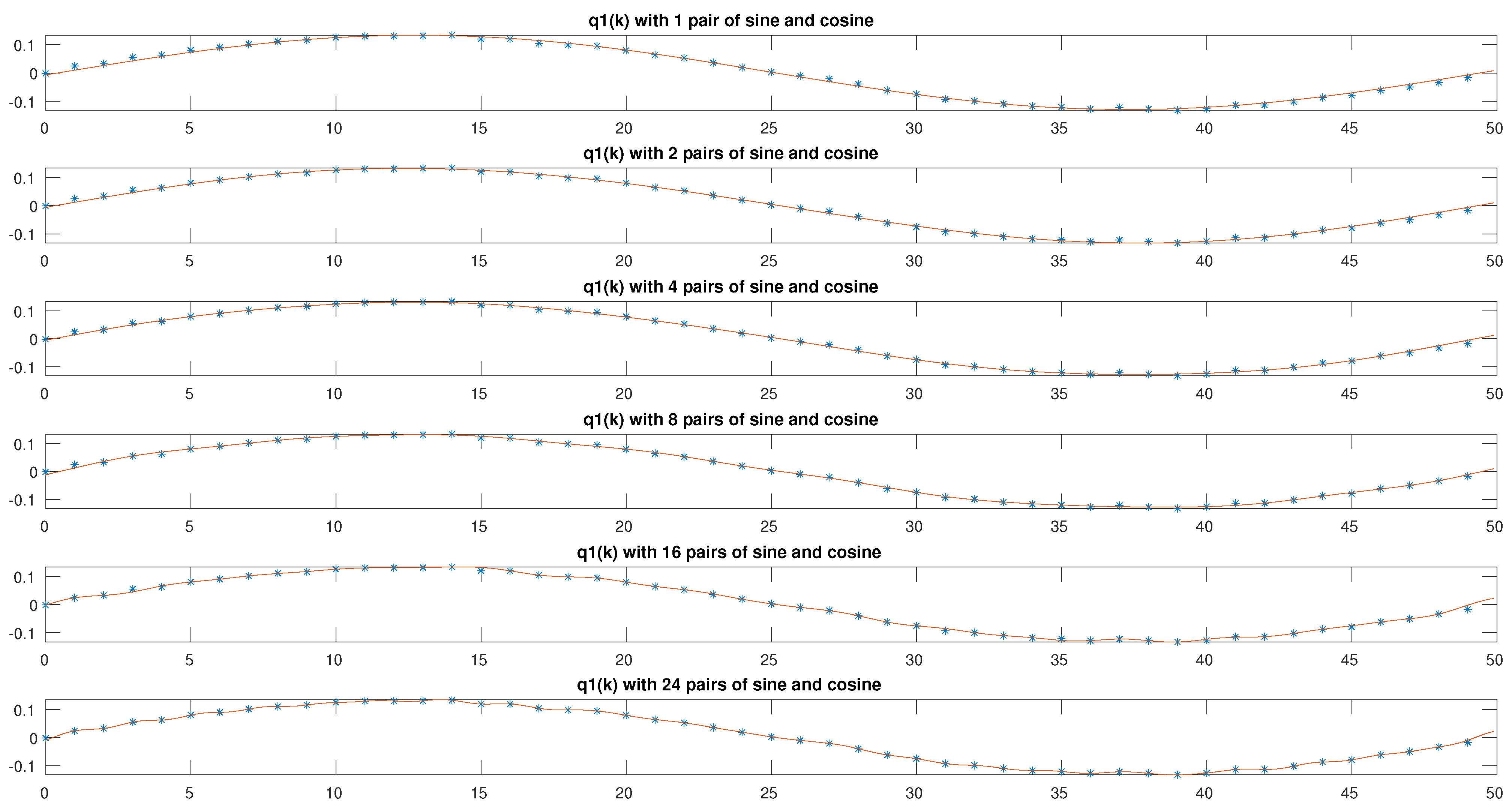
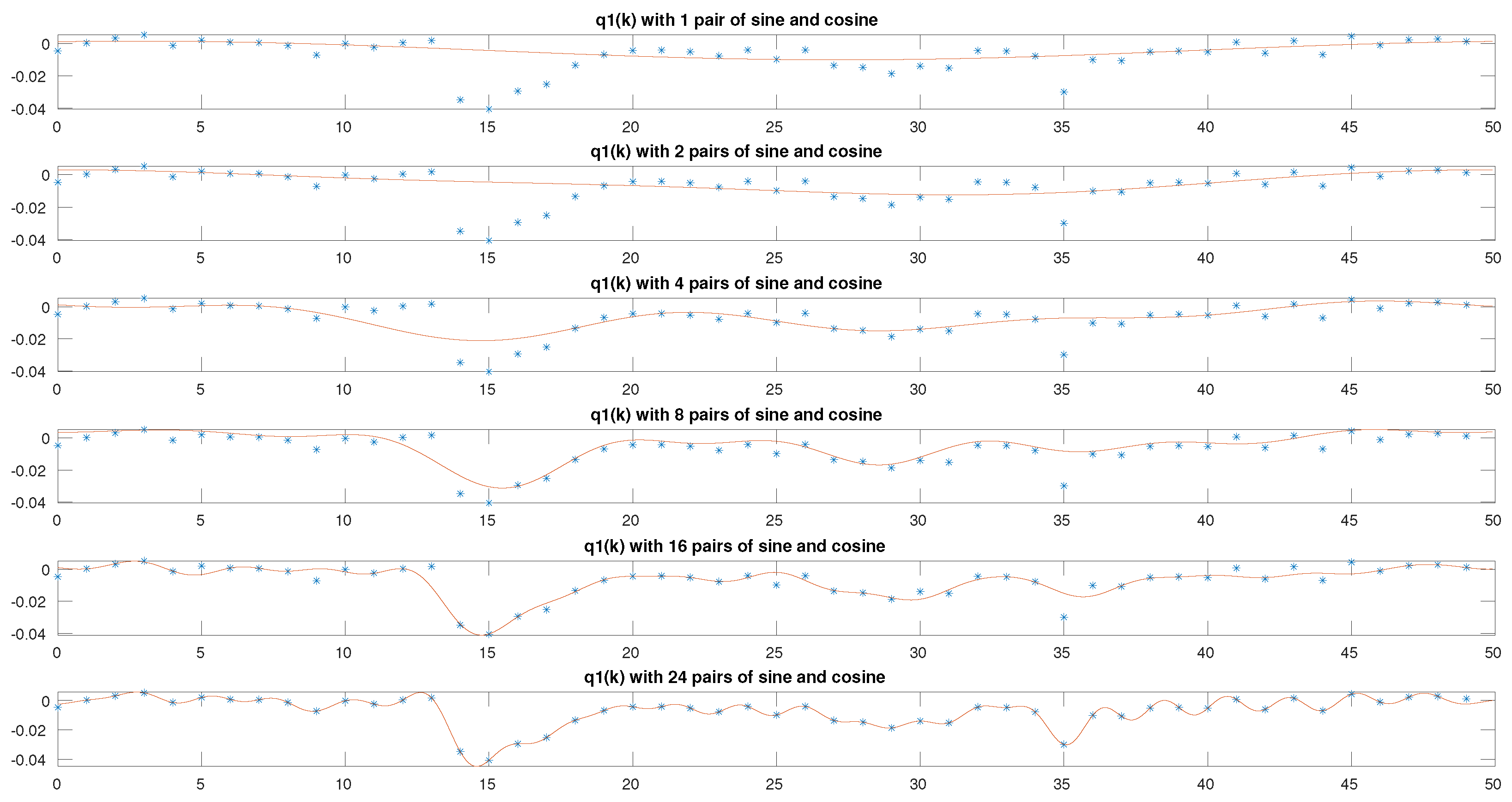
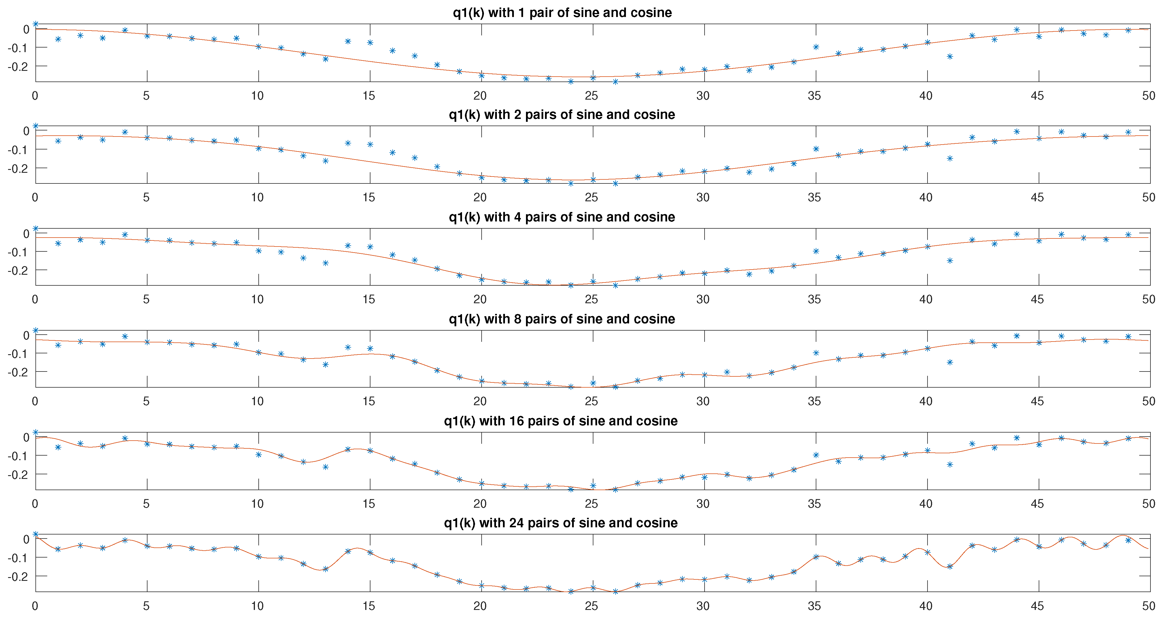
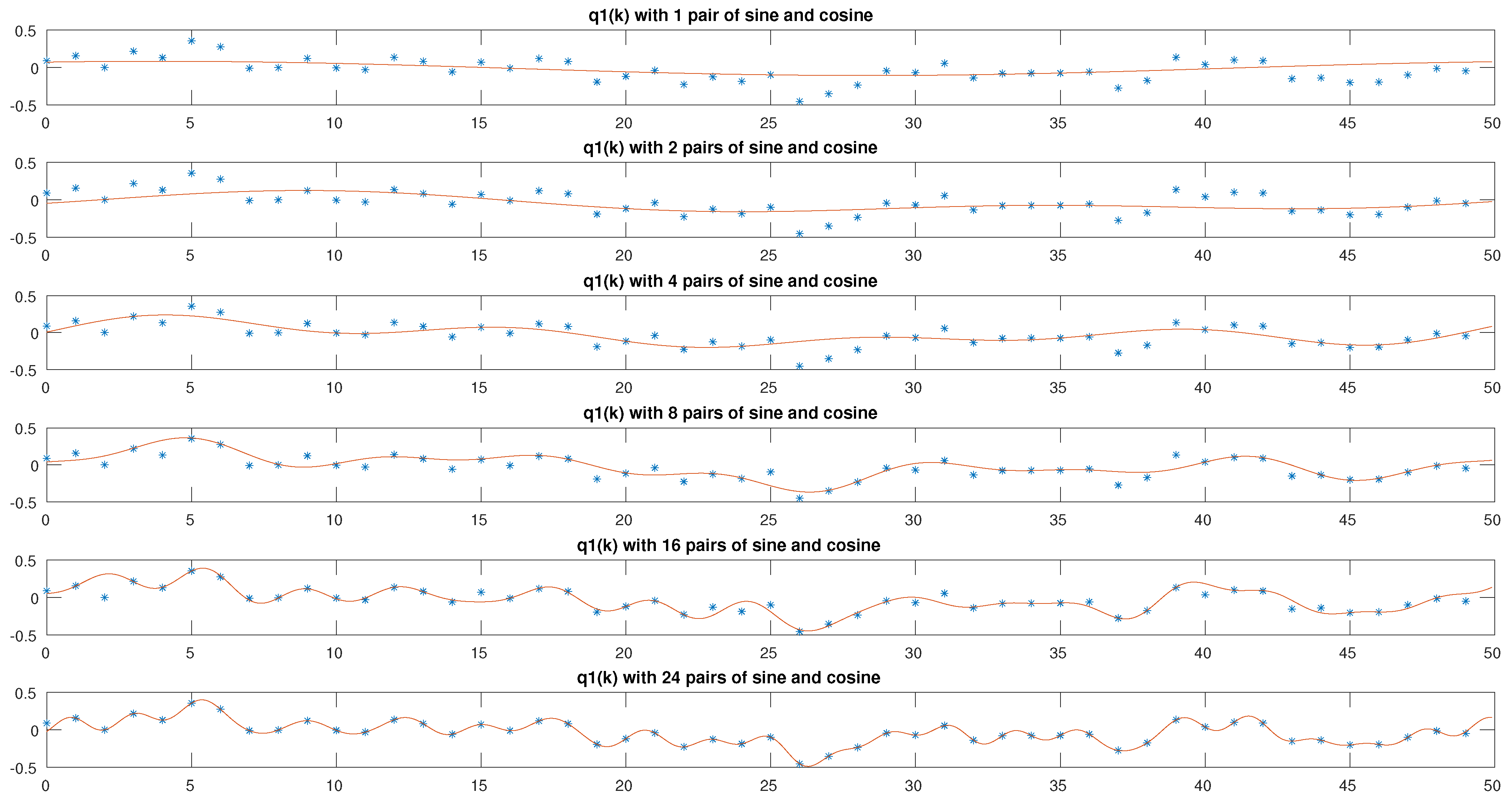
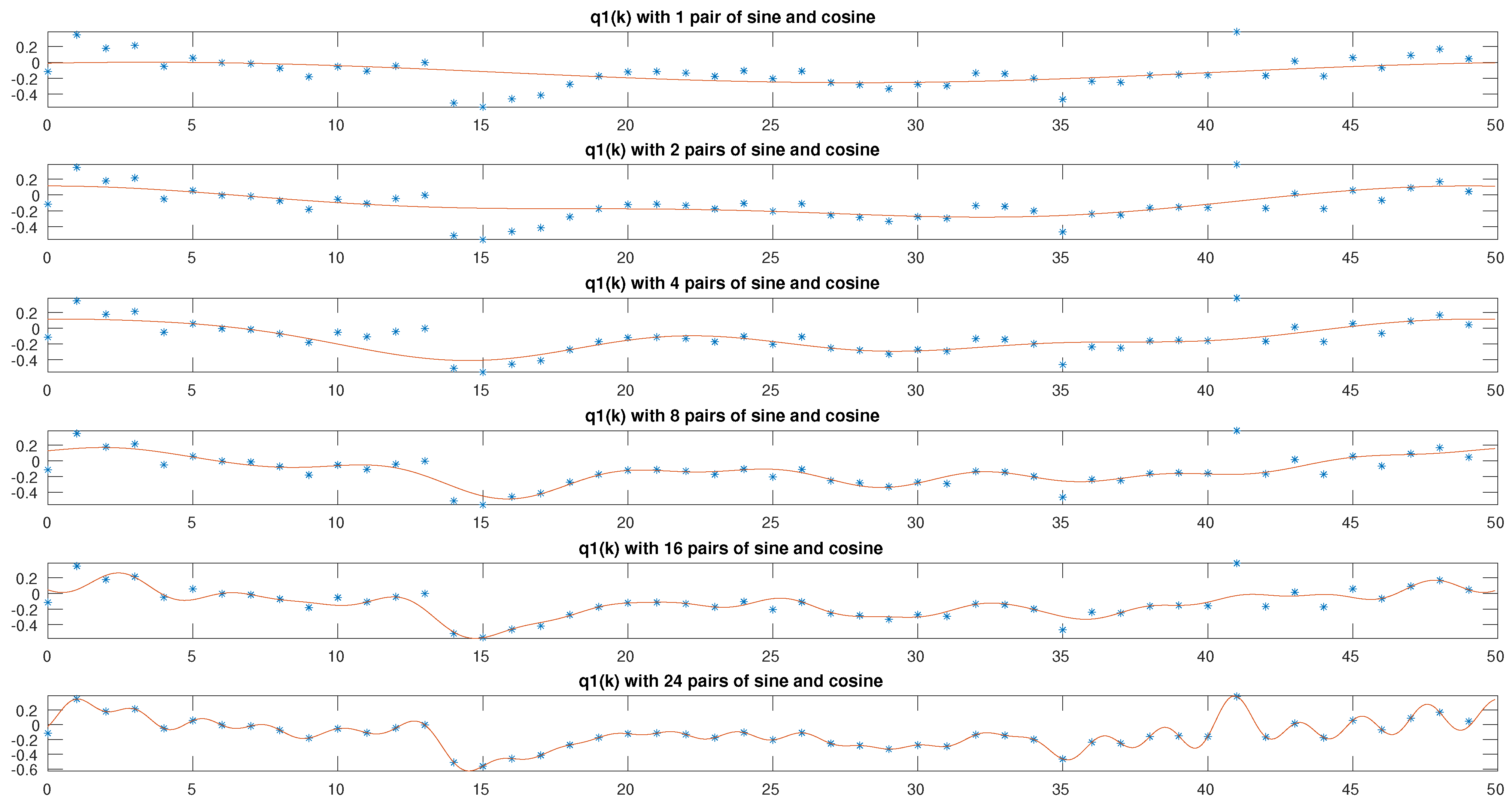
After solving the sequence of optimization problems related to the IKP for the path, the DE was used to identify the mathematical model using the Fourier representation. For each joint, different identifications were made by considering a number of finite terms of the Fourier series. The number of terms is defined by the number of sine and cosine pairs m in Expression (16), e.g., for , there are seven parameters to identify, . After each identification, the number of pairs is duplicated until 16 pairs are obtained (to find a vector solution with 33 variables). Different values of m were used to decrease the error until a value of the objective function of less than 0.1 was obtained or a maximum of 49 terms (m were obtained in the identified model. Table 3 shows the values of the error function for each of the links according to the number of parameters. Table 4 shows the values of the best identification for the function of joints .

Table 3.
Identification errors for each joint.

Table 4.
Values of the identification for joints .
For the particular case of Joint 6, it does not affect the position of any joint or the final effector in the inverse kinematics, but it does affect the orientation this joint, which was initialized at a value of 0 and remained at the same value throughout the trajectory. Figure 8, Figure 9, Figure 10, Figure 11 and Figure 12 show a representation of the trajectory made by the robot with the model identified for each joint with different m values (sine and cosine pair in Fourier representation).
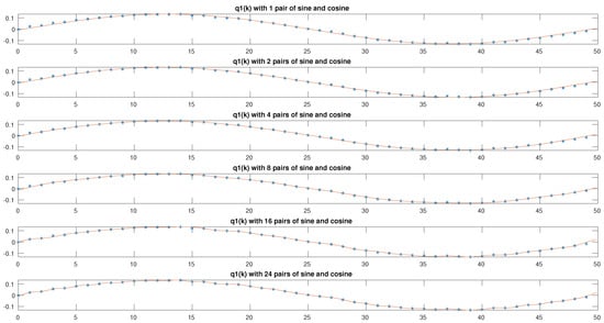
Figure 8.
The dotted graphs show the values for the q1 effector obtained in the trajectory as result of solving the optimization problem linked to the IKP, while the solid line is the representation of the identified model.
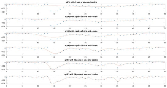
Figure 9.
The dotted graphs show the values for the q2 effector obtained in the trajectory as result of solving the optimization problem linked to the IKP, while the solid line is the representation of the identified model.
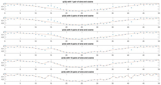
Figure 10.
The dotted graphs show the values for the q3 effector obtained in the trajectory as result of solving the optimization problem linked to the IKP, while the solid line is the representation of the identified model.
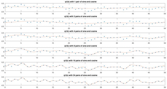
Figure 11.
The dotted graphs show the values for the q4 effector obtained in the trajectory as result of solving the optimization problem linked to the IKP, while the solid line is the representation of the identified model.
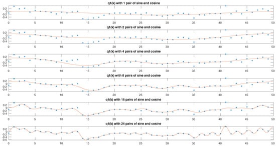
Figure 12.
The dotted graphs show the values for the q5 effector obtained in the trajectory as result of solving the optimization problem linked to the IKP, while the solid line is the representation of the identified model.
3.3. Discussion
From the first experiment, it is observed that the approach proposed in this work decreases the error for the furthest points in the trajectory, which correspond to the central points in the graphs of Figure 6 and Figure 7. This is of special importance for the identification of a model that describes the movement of the effectors, since a greater number of points with very wide errors generates a greater amount of unwanted data.
Although for experiment 2, all the points obtained from the optimization approach were preserved to solve the IKP, those with errors beyond a given tolerance could be eliminated, or the problem could be solved iteratively at those specific points, taking the information from the previous and next point as a starting point.
The identification was able to obtain a series of models that minimize the error between the samples and the mapped value at the same instants. In particular, with greater numbers of sines and cosines, the error in the objective function was reduced. Because the identification depends on the values obtained in the previous stage, it is important to start from the best result obtained through multiple executions since the proposal does not consider which are the most relevant points (with the least error) to be considered.
On the other hand, it is advisable to have different models, since in the case of the first effector (q1) with a single sine and cosine pair, a curve with a relatively small error is obtained, with a small difference with respect to the other models obtained. For the other joints, it is necessary to use a greater number of partners.
Although the application of the identification proposal arose from the field of robotics, it can be extended to other areas as long as it is a periodic function or it is limited to a domain in such a way that the values outside it are not relevant to the application and therefore are not used.
The method for solving the IKP is limited by the description of the robot through homogeneous transformations. This implies that parallel robots—in which it is usually required to solve an inverse kinematics problem simultaneously—are outside the scope of the proposal presented in this work. This constraint also implies its main contribution, since this proposal explores all admissible values for the robot effectors and then maps the values in Cartesian space to establish an error function so it does not suffer from the effects of dividing by zero. This is a common phenomenon in analytical approaches, whose advantage is the immediate response, but its implementation in robot controllers blocks the movement when found in points with multiple solutions, while the DE algorithm with a biased population chooses based on the influence of the previous posture.
The results obtained show the effectiveness of the proposed method. The efficiency is good since, despite the fact that the method works offline, the process of solving the IKP of the trajectory only takes approximately one hour in the worst case (maximum number of iterations criterion) with the computing system used. Additionally, once the functional model is obtained, it can be used for specific analyses associated with other areas not addressed in this work, such as robot dynamics.
A major limitation of this proposal is that it works offline because of the high number of iterations required to solve the IKP and to find the tuning. However, the advantage is that once the model is obtained, it can be used to analyze the differential kinematics of the trajectory tracking process. The proposed methodology also has the limitation of the type of robots in which it can be implemented, specifically serial robots, as a consequence of using homogeneous transformations and the Denavit–Hartenberg convention. In parallel robots, the constraints imposed by the closed loops require a different approach. Finally, the proposal only considers kinematic aspects, so the use of loads on the robot’s end effector could generate a dynamic singularity.
4. Conclusions
This work presents a methodology for solving the inverse kinematics problem of a serial robot as well as an identification process using an optimization approach and the differential evolution algorithm. A modification in the initialization of the DE algorithm was presented which consisted of biasing the population, taking into account the previous posture of the robot and the initial one based on the distance between the initial position of the effector and that of the current problem associated with the points of a closed trajectory. For the case study (Fanuc M-200 robot), a better result both in the average and in its variance textcolorblue(mean 11.0166 dynamic approach, mean 40.3967 fixed approach) was obtained because it is a weighted value that represents the 50 points that constitute the trajectory, corresponding to approximately 0.22 mm per point. As an additional contribution, the identification model based on metaheuristics and the Fourier series was able to find different functions that represent the movement of effectors with errors below 0.22 radians for the whole path of each effector.
As future work, it is considered to use techniques to prioritize points with the lowest error rates in the first stage of the identification process, as well as to implement additional considerations for other robots. It is also suggested to consider the physical constraints of the robot during the solution process. Additionally, it is necessary to explore the compatibility of the operators with other metaheuristic techniques in order to detect elements that facilitate the solution of the IKP.
Author Contributions
R.L.-M. and M.A.L.-P. worked on all the tasks, M.C.M.-R. and L.G.C.-R. worked on the literature review, R.L.-M. and M.A.L.-P. conducted experimental studies, E.V.-A. and L.G.C.-R. supervised. All authors analyzed the results. All authors have read and agreed to the published version of the manuscript.
Funding
This research received no external funding.
Data Availability Statement
The original contributions presented in this study are included in the article; further inquiries can be directed to the corresponding authors.
Conflicts of Interest
The authors declare no conflicts of interest.
References
- Reyes, F. Robotica—Control de Robots Manipuladores; Alfaomega Grupo Editor: Mexico City, Mexico, 2011. [Google Scholar]
- Ogbemhe, J.; Mpofu, K.; Tlale, N. Continuous Trajectory Planning for Welding of Complex Joints Using Bezier Curve. Procedia Manuf. 2019, 33, 685–692. [Google Scholar] [CrossRef]
- Javaid, M.; Haleem, A.; Singh, R.P.; Suman, R. Substantial capabilities of robotics in enhancing industry 4.0 implementation. Cogn. Robot. 2021, 1, 58–75. [Google Scholar] [CrossRef]
- Habibkhah, F.; Moallem, M. Application of machine learning for seam profile identification in robotic welding. Mach. Learn. Appl. 2025, 20, 100633. [Google Scholar] [CrossRef]
- Zhao, J.; Tian, Z.; Zhao, Z.; Yang, X.; Zhao, L.; Jiang, Z.; Liu, H. Constraint-integrated inverse kinematics method for dual-arm motion. Acta Astronaut. 2025, 228, 755–768. [Google Scholar] [CrossRef]
- Chen, F.; Ju, H.; Wang, K.; Cai, N. An analytical approach based on Dixon resultant for the inverse kinematics of 6R robot manipulators with offset wrists. Commun. Nonlinear Sci. Numer. Simul. 2023, 127, 107541. [Google Scholar] [CrossRef]
- Chen, F.; Ju, H.; Liu, X. Inverse kinematic formula for a new class of 6R robotic arms with simple constraints. Mech. Mach. Theory 2023, 179, 105118. [Google Scholar] [CrossRef]
- Wang, D.; Wu, J.; Wang, L.; Liu, Y. A Postprocessing Strategy of a 3-DOF Parallel Tool Head Based on Velocity Control and Coarse Interpolation. IEEE Trans. Ind. Electron. 2018, 65, 6333–6342. [Google Scholar] [CrossRef]
- Cagigas-Muñiz, D. Artificial Neural Networks for inverse kinematics problem in articulated robots. Eng. Appl. Artif. Intell. 2023, 126, 107175. [Google Scholar] [CrossRef]
- Diprasetya, M.R.; Pöppelbaum, J.; Schwung, A. KineNN: Kinematic Neural Network for inverse model policy based on homogeneous transformation matrix and dual quaternion. Robot. Comput.-Integr. Manuf. 2025, 94, 102945. [Google Scholar] [CrossRef]
- Amar, J.; Nagase, K. Genetic-algorithm-based global design optimization of tree-type robotic systems involving exponential coordinates. Mech. Syst. Signal Process. 2021, 156, 107461. [Google Scholar] [CrossRef]
- Abdor-Sierra, J.A.; Merchán-Cruz, E.A.; Rodríguez-Cañizo, R.G. A comparative analysis of metaheuristic algorithms for solving the inverse kinematics of robot manipulators. Results Eng. 2022, 16, 100597. [Google Scholar] [CrossRef]
- Ghosh, A.; Singh, O.; Ray, A.K. Inverse Kinematic Solution of a 7 DOF Robotic Manipulator using Boundary Restricted Particle Swarm Optimization. IFAC-PapersOnLine 2022, 55, 101–105. [Google Scholar] [CrossRef]
- López-Muñoz, R.; Portilla-Flores, E.A.; Corona-Ramírez, L.G.; Vega-Alvarado, E.; Maya-Rodríguez, M.C. Inverse Kinematics: An Alternative Solution Approach Applying Metaheuristics. Appl. Sci. 2023, 13, 6543. [Google Scholar] [CrossRef]
- Bouzgou, K.; Ahmed-Foitih, Z. Workspace Analysis and Geometric Modeling of 6 DOF Fanuc 200IC Robot. Procedia-Soc. Behav. Sci. 2015, 182, 703–709. [Google Scholar] [CrossRef][Green Version]
- Demby’s, J.; Gao, Y.; DeSouza, G.N. A Study on Solving the Inverse Kinematics of Serial Robots using Artificial Neural Network and Fuzzy Neural Network. In Proceedings of the 2019 IEEE International Conference on Fuzzy Systems (FUZZ-IEEE), New Orleans, LA, USA, 23–26 June 2019; pp. 1–6. [Google Scholar] [CrossRef]
- Thomas, F.; Porta, J.M. The inverse kinematics of lobster arms. Mech. Mach. Theory 2024, 196, 105630. [Google Scholar] [CrossRef]
- FANUC Robotics. LR Mate 200iC Series & R-30iA Mate Controller. 2009. Available online: https://www.fanucamerica.com/cmsmedia/datasheets/LR%20Mate%20200iC%20Series_10.pdf (accessed on 2 February 2025).
- Bouzgou, K.; Ahmed-Foitih, Z. Geometric modeling and singularity of 6 DOF Fanuc 200IC robot. In Proceedings of the Fourth edition of the International Conference on the Innovative Computing Technology (INTECH 2014), London, UK, 13–15 August 2014; pp. 208–214. [Google Scholar] [CrossRef]
- Gnetchejo, P.J.; Ndjakomo Essiane, S.; Dadjé, A.; Mbadjoun Wapet, D.; Ele, P. Optimal design of the modelling parameters of photovoltaic modules and array through metaheuristic with Secant method. Energy Convers. Manag. X 2022, 15, 100273. [Google Scholar] [CrossRef]
- Mao, Z.; Sun, Y.; Fang, K.; Huang, D.; Zhang, J. Model and metaheuristic for human–robot collaboration assembly line worker assignment and balancing problem. Comput. Oper. Res. 2024, 165, 106605. [Google Scholar] [CrossRef]
- Goud, H.; Sharma, P.C.; Nisar, K.; Reazul Haque, M.; Ibrahim, A.A.A.; Yadav, N.S.; Swarnkar, P.; Gupta, M.; Chand, L. Metaheuristics Algorithm for Tuning of PID Controller of Mobile Robot System. Comput. Mater. Contin. 2022, 72, 3481–3492. [Google Scholar] [CrossRef]
- Chandan, S.; Shah, J.; Singh, T.P.; Shaw, R.N.; Ghosh, A. Chapter Two—Inverse kinematics analysis of 7-degree of freedom welding and drilling robot using artificial intelligence techniques. In Artificial Intelligence for Future Generation Robotics; Shaw, R.N., Ghosh, A., Balas, V.E., Bianchini, M., Eds.; Elsevier: Amsterdam, The Netherlands, 2021; pp. 15–23. [Google Scholar] [CrossRef]
- Price, K.; Storn, R.M.; Lampinen, J.A. Differential Evolution: A Practical Approach to Global Optimization; Springer Science & Business Media: Berlin/Heidelberg, Germany, 2006. [Google Scholar]
- Gao, W.-F.; Liu, S.-y. A modified artificial bee colony algorithm. Comput. Oper. Res. 2012, 39, 687–697. [Google Scholar] [CrossRef]
- Serov, V. Fourier Series, Fourier Transform and Their Applications to Mathematical Physics; Springer: Berlin/Heidelberg, Germany, 2017; Volume 197. [Google Scholar]
- Das, S.; Suganthan, P.N. Differential Evolution: A Survey of the State-of-the-Art. IEEE Trans. Evol. Comput. 2011, 15, 4–31. [Google Scholar] [CrossRef]
- Cerulli, M.; D’Ambrosio, C.; Liberti, L. Flying Safely by Bilevel Programming. In Advances in Optimization and Decision Science for Society, Services and Enterprises: ODS, Genoa, Italy, 4–7 September 2019; Springer International Publishing: Cham, Switzerland, 2019; pp. 197–206. [Google Scholar] [CrossRef]
Disclaimer/Publisher’s Note: The statements, opinions and data contained in all publications are solely those of the individual author(s) and contributor(s) and not of MDPI and/or the editor(s). MDPI and/or the editor(s) disclaim responsibility for any injury to people or property resulting from any ideas, methods, instructions or products referred to in the content. |
© 2025 by the authors. Licensee MDPI, Basel, Switzerland. This article is an open access article distributed under the terms and conditions of the Creative Commons Attribution (CC BY) license (https://creativecommons.org/licenses/by/4.0/).

