Optimal Investment Based on Performance Measure and Stochastic Benchmark Under PI and Position Constraints

Abstract

We consider the portfolio selection problem faced by a manager under the performance ratio with position and portfolio insurance (PI) constraints. By making use of a dual control method in an incomplete market setting, we find the unique pricing kernel in the presence of closed convex cone control constraints. Then, following the same arguments as in the complete market case, we derive the explicit form of the optimal investment strategy by combining the linearization method, the Lagrangian method, and the concavification technique.

1. Introduction

In the past decade, the Omega ratio, proposed by [1], has received increasing attention both from academics and practitioners as an alternative to the classical Sharpe ratio [2,3,4] when measuring the performance of different investment opportunities; see [5,6,7,8]. The Omega ratio can be interpreted as a return–risk ratio. The return is measured as the expected gain above a given threshold whereas risk is measured as the expected loss below the same threshold. Since only adverse deviations from the threshold contribute to the risk component of the Omega ratio, this measure is particularly attractive for situations where the return distribution is strongly asymmetric. The Omega ratio is deemed a better performance measurement than the Sharpe ratio which measures risk by the standard deviation since this measure effectively distinguishes between upward and downward deviations from the benchmark. Furthermore, in contrast to the Sharpe ratio which only considers the portfolio return’s first- and second-order moments, it accounts for higher-order information contained in returns.

However, as pointed out by [9,10], the optimization problem based on the Omega ratio is ill-posed. Therefore, Lin et al. [10] modify the Omega ratio to include a reward function for over-performance and a penalty function for under-performance in the definition of the performance ratio. They investigate the optimization problem of maximizing the extended Omega ratio. Based on the fractional programming method, they analyze the non-linear fractional optimization problem by solving a family of related non-fractional optimization problems, where the objective functions are the numerator of the original problem minus the denominator multiplied by a penalty parameter. Since they work in a complete financial market, there exists a unique pricing kernel and therefore the martingale method can be directly used to solve the optimization problem, which involves solving a terminal static optimization problem first to obtain the optimal terminal wealth and then identifying the portfolio strategy that replicates the optimal terminal wealth; see [11,12,13,14]. From a risk management point of view, the under-performance should be controlled by incorporating a risk constraint. Therefore, Guan et al. [15] extend [10] to include a value-at-risk (VaR) constraint.

In [10,15], the benchmark is set to be a constant, which is equivalent to a money account. Actually, the choice of the benchmark which measures over-performance and under-performance plays an important role in the performance measure optimization problem. Typically, a benchmark represents a general indicator of market sentiment. A specific choice for the benchmark falls into three usual categories: a portfolio, an index, or any economic indicator. Ng and Nguyen [16] investigate an optimization problem with a stochastic benchmark based on a different performance measure, in which the performance measure is defined as the Omega ratio of the utility of the portfolio with respect to the utility of the benchmark, which quantifies utility gain over utility loss of the portfolio performance relative to the benchmark. Ng and Nguyen [16] derive the optimal solution in a complete market setting, when the benchmark is set to be a non-increasing function of the market price density. However, for an incomplete market model setting with infinitely many pricing kernels, the method adopted by [16] loses effectiveness. Tang et al. [17] generalize [10] to a performance measure optimization problem with a stochastic benchmark faced by a fund manager. For a general stochastic benchmark, it is difficult to derive the closed-form solution for the performance measure maximization problem. When the reward and penalty functions are both power functions, Tang et al. [17] derive the explicit investment strategy of a performance measure optimization problem with a stochastic benchmark, which is set to be a value-weighted portfolio with a fixed proportion invested in the risky asset. However, for other choices of reward and penalty functions, the stochastic benchmark considered in [17] does not allow to explicitly derive the optimal solution. We consider a stochastic benchmark which allows for closed-form solutions to a performance measure optimization problem for general reward and penalty functions. As suggested in [15], in order to improve the performance of the fund under downside risk, a risk constraint should be incorporated into the optimization model. The portfolio insurance (PI) constraint requires the manager to keep the terminal wealth above a minimum guarantee, which is essential for the welfare of the investors. Risk management using PI constraint has been investigated in a lot of works; see [18,19,20]. In this paper, we investigate the optimal investment problem of a fund manager based on performance measure under PI and position constraints.

However, there may be some position constraints on the investment possibilities in the real world by financial regulations. In the case of control constraints, the martingale method may lose its effectiveness as the financial market is not complete and explicit solutions have been obtained for only a few special cases. The martingale approach has been generalized by a number of researchers using stochastic duality theory to explicitly solve the optimization problems when the portfolio shares are restricted to lie in a closed convex cone, including prohibiting from investing in or no-short-selling some risky assets. For a concave utility maximization problem, He and Zhou [21] show that there exists a unique pricing kernel, called the minimal pricing kernel, in the presence of closed convex cone control constraints. So, one may solve the position-constrained problem in the same way as in the complete market case. Dong and Zheng [22] use the dual control method to find the unique pricing kernel and then solve the non-concave utility maximization problem with closed convex cone control constraints. In this paper, we incorporate position constraints into the performance measure maximization problem.

This paper is related to [17], where the authors study the performance measure optimization with a stochastic benchmark. However, our paper is different from theirs at least in two aspects. First, we propose a different stochastic benchmark, which allows to explicitly solve the optimization problem for general reward and penalty functions. Furthermore, the stochastic benchmark in [17], which is a value-weighted portfolio with a fixed proportion invested in the risky asset, can be deemed to be exogenously given. Therefore, the manager’s risk-taking choices are highly influenced by the referenced portfolio. As shown in [17], there is a tendency for the manager to gambling with excess risk-taking when the benchmark allocates a higher proportion of wealth in the risky asset. Different from [17], the stochastic benchmark in this paper is updated according to the development of the wealth process, which implies that the benchmark is mainly driven by preferences of the investor. Second, due to the concern about a downside protection and regulations on the investment possibilities, we introduce minimum performance and position constraints, which are not considered in their paper. These constraints lead our model to be more complicated than theirs and help us to learn more of the characteristics of the fund manager’s investment behavior.

The main contribution of this paper is that motivated by [10,18,22]. We investigate the optimal allocation problem based on performance measure with a stochastic benchmark under PI and position constraints. The present paper not only contributes to the literature on the optimal portfolio selection based on performance measure, but also explores the connection between the S-shaped utility maximization problem with the performance measure optimization problem.

The rest of the paper is organized as follows. In Section 2, we formulate an optimal allocation problem by maximizing a performance measure with a stochastic benchmark under PI and position constraints. In Section 3, we apply the linearization method, the martingale method, and the concavification technique to derive the optimal solution. In Section 4, we numerically investigate the impacts of some model parameters on the optimal terminal wealth and the optimal investment strategy. Section 5 concludes the paper. Appendix A contains related proofs.

2. The Model

We consider a finite investment time horizon $[0,T]$ with $T>0$ and a continuous-time financial market without transaction costs. We let $(\mathcal{N},\mathcal{F},\mathbb{F},P)$ be a filtered complete probability space, in which the filtration $\mathbb{F}:=\left\{{\mathcal{F}}_t\right|0\le t\le T\}$ is P-augmented filtration induced by an n-dimensional standard Brownian motion $W\left(t\right)={(W_1\left(t\right),\cdots ,W_n\left(t\right))}^{\top },$ where $W_1\left(t\right),\cdots ,$$W_n\left(t\right)$ are mutually independent and $a^{\top }$ is the transpose of $a.$

We consider a financial market with n risky assets, denoted by $S\left(t\right)={(S_1\left(t\right),\cdots ,S_n\left(t\right))}^{\top }$, and a risk-free security $S_0\left(t\right)$, which accrues interest continuously at the risk-free rate $r\ge 0$.

It is assumed that under the real-world probability measure $P,$ the price process of the risk-free security evolves as

$$\begin{array}{c}\hfill {\displaystyle \frac{d{S}_0\left(t\right)}{S_0\left(t\right)}}=rdt.\end{array}$$

(1)

The price processes of the n risky assets are modeled by

$$\begin{array}{c}\hfill dS\left(t\right)=\mathrm{diag}\left(S\right(t\left)\right)(\mu dt+\sigma dW(t\left)\right),\end{array}$$

(2)

where $S\left(t\right)={(S_1\left(t\right),\cdots ,S_n\left(t\right))}^{\top }$, $\mathrm{diag}\left(S\right(t\left)\right)$ is an $n\times n$ matrix with diagonal elements $S_i\left(t\right)$ and all other elements 0, $\mu ={({\mu }_1,\cdots ,{\mu }_n)}^{\top }$ is a constant vector representing the stock growth rate with ${\mu }_i>r,i=1,\cdots ,n,$ and $\sigma =\left({\sigma }_{ij}\right)$ is an $n\times n$ nonsingular constant matrix representing the volatility and correlation information of $S\left(t\right).$

Suppose that the initial wealth of the fund account is $x_0⩾0.$ The fund manager invests the wealth in a risk-free asset and n risky assets. We let ${\pi }_i\left(t\right)$ be the proportion of wealth invested in the ith risky asset at time t for $i=1,\cdots ,n.$ The remaining proportion $1-{\displaystyle \sum _{i=1}^n}{\pi }_i\left(t\right)$ of wealth is invested in the risk-free security. We let $\pi \left(t\right)={({\pi }_1\left(t\right),\cdots ,{\pi }_n\left(t\right))}^{\top }.$ With the trading strategy $\pi =\left\{\pi \right(t),0\le t\le T\},$ the wealth process $X^{\pi }\left(t\right)$, denoted by $X^{\pi }\left(t\right)$, evolves according to the following stochastic differential equation (SDE):

$$\begin{array}{c}\hfill d{X}^{\pi }\left(t\right)=X^{\pi }\left(t\right)(r+{\pi }^{\top }\left(t\right)\sigma \xi )dt+X^{\pi }\left(t\right){\pi }^{\top }\left(t\right)\sigma dW\left(t\right),X^{\pi }\left(0\right)=x_0\ge 0,\end{array}$$

(3)

where $\xi ={\sigma }^{-1}(\mu -r\mathbf{1})$ and $\mathbf{1}$ denotes the n-dimensional column vector with each element equal to 1. It is natural to assume that the trading strategy $\pi ={({\pi }_1,\cdots ,{\pi }_n)}^{\top }$ is $\mathcal{F}$-progressively measurable and satisfies $E[{\int }_0^T\parallel \pi \left(t\right){\parallel }^{2}dt]<\infty$ almost surely so that there exists a unique strong solution $X^{\pi }\left(t\right)$ to (3) where ${\parallel .\parallel }^2$ denotes the $L^2$-norm.

Definition 1.

We let K be a closed convex cone. A portfolio strategy $\pi ={({\pi }_1,\cdots ,{\pi }_n)}^{\top }$ is said to be admissible if it is a progressively measurable, $\mathcal{F}$-adapted process which satisfies $E[{\int }_0^T\parallel \pi \left(t\right){\parallel }^{2}dt]<\infty$, $\pi \left(t\right)\in K$ almost surely and there exists a unique strong solution $X^{\pi }\left(t\right)$ to (3). The set of all admissible portfolio strategies is denoted by $\mathcal{A}$.

The literature on portfolio performance evaluation starts with the Sharpe ratio (see [3]). Alternative performance measures are reward-to-risk ratios representing a fraction where a measure of reward is divided by a measure of risk. Examples of such reward-to-risk ratios include the Omega ratio (see, e.g., [1]) and the extended Omega ratio (see, e.g., [10]). Based on [1,10], we first formally define the performance measure in this paper and next aim at finding the optimal portfolios that have maximum performance measure.

The Omega ratio for a random payoff $X^{\pi }\left(T\right)$ with respect to the benchmark $\theta \left(T\right)$ is defined as

$${\Omega }_{\theta }\left(X^{\pi }\left(T\right)\right)={\displaystyle \frac{E\left[{(X^{\pi }\left(T\right)-\theta )}_{+}\right]}{E\left[{(\theta -X^{\pi }\left(T\right))}_{+}\right]}},$$

(4)

where ${\left(x\right)}_{+}=max(x,0).$

The Omega ratio is better than the Sharpe ratio since it measures the ratio between the upper tail heaviness (from $\theta \left(T\right)$ onwards) and the corresponding lower tail heaviness (below the level $\theta \left(T\right)$). However, as shown in [9,10], the maximization problem of the Omega ratio is ill-posed due to the linear growth of its numerator. To make the optimization problem bounded, Lin et al. [10] propose a “utility-transformed” Omega ratio by introducing two weighting functions. We follow the framework in [10] and introduce a reward function $U\left(x\right)$ over gains and a penalty function $D\left(x\right)$ over losses for the manager, respectively. Therefore, the performance measure in our paper is defined by

$${\Omega }_{\theta }\left(X^{\pi }\left(T\right)\right)={\displaystyle \frac{E\left[U{(X^{\pi }\left(T\right)-\theta \left(T\right))}_{+}\right)]}{E\left[D{(\theta \left(T\right)-X^{\pi }\left(T\right))}_{+}\right)]}},$$

(5)

where U and D are two monotonically increasing measurable functions. The performance measure defined in (5) distinguishes the gains and losses by the benchmark $\theta \left(T\right)$ and shows that the manager has different attitudes towards gains and losses. In general, the reward function U is strictly concave since the decision-makers are usually risk-averse towards gains. However, as discussed in [23], the decision-makers may have two different attitudes towards the losses: risk aversion and loss aversion. When the penalty function D is convex, the manager is risk-averse towards the losses. When the penalty function is concave, the manager is loss-averse, which is first proposed by [24] within the framework of prospect theory. Berkelaar et al. [23] analyze the optimal investment strategy for loss-averse investors. In what follows, we assume that U is a strictly concave function, and D is either concave or convex.

Lin et al. [10] derive the optimal solution under the assumption that the investor has a constant benchmark for distinguishing losses and gains and there are no constraints on the terminal wealth and trading positions. It seems more plausible that an investor dynamically updates their benchmark according to the development of his wealth. We assume that at initial time the investor is assumed to have an initial reference point $\theta \left(0\right)$; then, the investor adjusts their initial reference point $\theta \left(0\right)$ with the constant risk-free interest rate r weighted by $1-\alpha$, and with the change in their wealth $d{X}^{\pi }\left(t\right)$ weighted by $\alpha$, where $\alpha \in [0,1)$ is a constant. As a result, the stochastic reference point evolves dynamically according to the process as follows:

$$\begin{array}{c}\hfill d\theta \left(t\right)=(1-\alpha )\theta \left(0\right)rdt+\alpha d{X}^{\pi }\left(t\right),t\ge 0,\theta \left(0\right)={\theta }_0.\end{array}$$

(6)

We formulate the manager’s portfolio selection problem as

$$\begin{array}{c}\hfill \left\{\begin{array}{c}\underset{\pi \in \mathcal{A}}{max}{\displaystyle \frac{E\left[U{(X^{\pi }\left(T\right)-\theta \left(T\right))}_{+}\right)]}{E\left[D{(\theta \left(T\right)-X^{\pi }\left(T\right))}_{+}\right)]}},\hfill \\ s.t.X^{\pi }\left(t\right)\mathrm{ssatisfies}\left(3\right),X^{\pi }\left(T\right)\ge H.\hfill \end{array}\right.\end{array}$$

(7)

The numerator $E{[U\left(X^{\pi }\left(T\right)\right)-\theta \left(T\right))}_{+}]$ measures the benefit from exceeding the benchmark wealth $\theta \left(T\right)$, while the denominator $E\left[D{(\theta \left(T\right)-X^{\pi }\left(T\right))}^{+}\right)]$ penalizes shortfalls.

Note that Equation (6) gives

$$\theta \left(T\right)=\theta \left(0\right)+(1-\alpha )\theta \left(0\right)rT+\alpha (X^{\pi }\left(T\right)-X^{\pi }\left(0\right)).$$

Hence,

$$\begin{array}{c}\hfill X^{\pi }\left(T\right)-\theta \left(T\right)=(1-\alpha )X^{\pi }\left(T\right)+\alpha x_0-\theta \left(0\right)-(1-\alpha )\theta \left(0\right)rT\widehat{=}(1-\alpha )X^{\pi }\left(T\right)-{\overline{\theta }}^{*},\end{array}$$

(8)

where ${\overline{\theta }}^{*}=-\alpha x_0+\theta \left(0\right)+(1-\alpha )\theta \left(0\right)rT.$ We assume that ${\overline{\theta }}^{*}>0$ and $H<{\displaystyle \frac{{\overline{\theta }}^{*}}{1-\alpha }}$ such that $P(X^{\pi }\left(T\right)<\theta \left(T\right))>0.$

Remark 1.

Equation (8) shows that the performance measure optimization problem related to the terminal wealth with a stochastic benchmark given by (6) is identical to the performance measure optimization problem related to the terminal wealth with a constant benchmark. Hence, the performance measure optimization problem with the stochastic benchmark we consider in this paper can be explicitly solved under general penalty and reward functions by using combining the linearization method, the Lagrangian method, and the concavification technique. However, the performance measure optimization problem over the terminal wealth with a stochastic benchmark investigated in [17] cannot be transformed into the performance measure optimization problem over the terminal wealth with a constant benchmark. When the penalty and reward functions are both set to be power functions with the same exponent γ, they use the change in measure method to relate the original optimization problem over the terminal wealth with a stochastic benchmark to the performance measure optimization problem over the relative terminal performance (i.e., the ratio of the terminal wealth and the stochastic benchmark) with a constant benchmark. For general reward and penalty functions, the method adopted by [17] losses its effectiveness.

By using (8), (7) can be rewritten as

$$\begin{array}{c}\hfill \left\{\begin{array}{c}\underset{\pi \in \mathcal{A}}{max}{\displaystyle \frac{\mathbb{E}\left\{U\left[{((1-\alpha )X^{\pi }\left(T\right)-{\overline{\theta }}^{*})}_{+}\right]\right\}}{\mathbb{E}\left\{D\left[{({\overline{\theta }}^{*}-(1-\alpha )X^{\pi }\left(T\right))}_{+}\right]\right\}}},\hfill \\ s.t.X^{\pi }\left(t\right)\mathrm{satisfies}\left(3\right),X^{\pi }\left(T\right)\ge H.\hfill \end{array}\right.\end{array}$$

(9)

When there are no constraints on the investment strategies, the market has a unique pricing kernel as follows:

$$H\left(t\right)=e^{-\left(r+{\displaystyle \frac{{\parallel \xi \parallel }^2}{2}}\right)t-{\xi }^{\top }W\left(t\right)},0⩽t⩽T.$$

However, in the case of control constraints, the market is no longer complete and there are many pricing kernels. Therefore, the traditional martingale method cannot be used to solve the optimization problem with control constraints. According to [22], there exists a unique pricing kernel in the presence of closed convex cone control constraints given by

$$\begin{array}{c}\hfill H^{\hat{\nu }}\left(t\right)=e^{-\left(r+{\displaystyle \frac{\parallel \hat{\xi }{\parallel }^2}{2}}\right)t-{\hat{\xi }}^{\top }W\left(t\right)},0⩽t⩽T,\end{array}$$

(10)

where

$$\hat{\xi }=\xi +{\sigma }^{-1}\hat{\nu },\hat{\nu }=\mathrm{argmin}\{\xi +{\sigma }^{-1}\nu ,\nu \in K^o\},$$

with $K^o=\{p\in R^n:p^{\prime }v⩾0,\forall v\in K\}$ being the positive cone of $K.$

From [7], once the pricing kernel is found, the optimization problem (9) can be transformed into an equivalent one with respect to the terminal wealth $Z\widehat{=}{X}^{\pi }\left(T\right)$:

$$\left\{\begin{array}{c}\underset{Z\in {\mathcal{M}}_{+}}{sup}{\displaystyle \frac{\mathbb{E}\left\{U\left[{((1-\alpha )Z-{\overline{\theta }}^{*})}_{+}\right]\right\}}{\mathbb{E}\left\{D\left[{({\overline{\theta }}^{*}-(1-\alpha )Z)}_{+}\right]\right\}}},\hfill \\ \mathrm{subject}\mathrm{to}\mathbb{E}\left[H^{\hat{\nu }}\left(T\right)Z\right]\le x_0,Z\ge H,\hfill \end{array}\right.$$

(11)

where ${\mathcal{M}}_{+}$ denotes the set of non-negative ${\mathcal{F}}_T$-measurable random variables. We denote the feasible set of the above problem by $\mathcal{C}\left(x_0\right)$:

$$\mathcal{C}\left(x_0\right)=\{Z\in {\mathcal{M}}_{+}\mid \mathbb{E}\left[H^{\hat{\nu }}\left(T\right)Z\right]\le x_0\}.$$

The following result states that we can first solve the terminal static optimization problem (11) over the random variable $Z\in {\mathcal{M}}_{+}$ and then find the optimal portfolio ${\pi }^{*}$ by the martingale representation theorem.

Theorem 1.

We assume that $Z^{*}$ is the optimal solution to Problem (11). Then, there exists a strategy ${\pi }^{*}\in \mathcal{A}$ such that $X^{{\pi }^{*}}\left(T\right)=Z^{*}$, almost surely.

Proof. 

See Appendix A. □

Theorem 1 shows that in order to solve Problem (7), we only need to investigate Problem (11) first.

Since the optimal payoff problem (11) involves a non-linear objective function, it is difficult to solve directly. In order to reformulate it into a tractable problem, we set up the following family of linearized problems parameterized by $\lambda \ge 0$:

$$v(\lambda ;x_0)=\underset{Z\in \mathcal{C}\left(x_0\right),Z\ge H}{sup}\mathbb{E}\left\{U\left[{((1-\alpha )Z-{\overline{\theta }}^{*})}_{+}\right]\right\}-\lambda \mathbb{E}\left\{D\left[{({\overline{\theta }}^{*}-(1-\alpha )Z)}_{+}\right]\right\}.$$

(12)

Remark 2.

Similar to the proof of Theorem 1, it is easy to verify that when Problem (12) attains the optimal value, the budget constraint is binding, that is,

$$v(\lambda ;x_0)=\underset{Z\in C^{\mathrm{eq}}\left(x_0\right),Z\ge H}{sup}\mathbb{E}\left\{U\left[{((1-\alpha )Z-{\overline{\theta }}^{*})}_{+}\right]\right\}-\lambda \mathbb{E}\left\{D\left[{({\overline{\theta }}^{*}-(1-\alpha )Z)}_{+}\right]\right\},$$

(13)

where

$$C^{\mathrm{eq}}\left(x_0\right):=\{Z\in {\mathcal{M}}_{+}|\mathbb{E}\left[H^{\hat{\nu }}\left(T\right)Z\right]=x_0\}.$$

We establish the relationship between linearized Problems (11) and (12).

Note that for a constrained optimization problem, the optimal solution may not exist for a relatively low value of initial wealth $x_0.$ To guarantee that optimization Problem (11) is feasible, we assume that $x_0\ge H{e}^{-rT}.$

Theorem 2.

We assume $H{e}^{-rT}<x_0<e^{-rT}{\displaystyle \frac{{\overline{\theta }}^{*}}{1-\alpha }}$. For each $\lambda \ge 0$, we let $Z_{\lambda }^{*}$ be a solution to Problem (12) and suppose there exists a constant ${\lambda }^{*}\ge 0$ such that

$${\lambda }^{*}={\displaystyle \frac{\mathbb{E}\left\{U\left[{((1-\alpha )Z_{{\lambda }^{*}}^{*}-{\overline{\theta }}^{*})}_{+}\right]\right\}}{\mathbb{E}\left\{D\left[{({\overline{\theta }}^{*}-(1-\alpha )Z_{{\lambda }^{*}}^{*})}_{+}\right]\right\}}}.$$

(14)

Then, $Z^{*}:=Z_{{\lambda }^{*}}^{*}$ solves Problem (11) and ${\lambda }^{*}$ is the optimal value.

Proof. 

See Appendix A. □

Remark 3.

Prospect theory, introduced by [24,25], is also concerned with gains and losses of a portfolio. Tversky and Kahneman [25] demonstrate the loss aversion and risk seeking behaviour by an asymmetric S-shaped utility function, convex in the domain of losses and concave in the domain of gains. In (12), if λ = 1, U and D are two concave functions, then (12) becomes an S-shaped utility maximization problem studied in [19]. Therefore, different from an S-shaped utility maximization problem, for a performance ratio optimization problem, D may be concave or convex and the optimal multiplier ${\lambda }^{*}$ should be determined by (14).

Within the framework of prospect theory, the power utilities are widely used to capture the preferences over gains and losses; see [22,25,26,27]. For simplicity, we follow [25] to consider U and D to be power utilities. However, the following theoretical analysis can also be applied for other choices of reward and penalty functions.

We let

$$U\left(x\right)=x^{{\gamma }_1},0<{\gamma }_1<1,D\left(x\right)=x^{{\gamma }_2},{\gamma }_2>0.$$

It is easy to check that U is strictly concave. For the weighting function D, we consider two cases: $0<{\gamma }_2\le 1$ and ${\gamma }_2>1$. Note that D is concave for $0<{\gamma }_2\le 1$ and convex for ${\gamma }_2>1,$ respectively.

It remains to show the existence and uniqueness of ${\lambda }^{*}.$ To this end, we need the following results.

Lemma 1.

We assume $H{e}^{-rT}<x_0<e^{-rT}{\displaystyle \frac{{\overline{\theta }}^{*}}{1-\alpha }}$. We define $M={sup}_{Z\in C^{\mathrm{eq}}\left(x_0\right)}\mathbb{E}\left[U\left({((1-\alpha )Z-{\overline{\theta }}^{*})}_{+}\right)\right]$ and $m={inf}_{Z\in C^{\mathrm{eq}}\left(x_0\right)}\mathbb{E}\left[D\left({({\overline{\theta }}^{*}-(1-\alpha )Z)}_{+}\right)\right]$. Then, $M<\infty$ and $m>0$.

Proof. 

See Appendix A. □

The following proposition presents some relevant properties of the value function v defined in (12).

Proposition 1.

We suppose that $H{e}^{-rT}\le x_0<{\displaystyle \frac{e^{-rT}{\overline{\theta }}^{*}}{1-\alpha }}$. Then, the function $v(\lambda ;x_0)$ has the following properties:

(a)

$0<v(0;x_0)<\infty .$

(b)

v is non-increasing in $\lambda .$

(c)

$v(\lambda ;x_0)\mathit{isconvexin}\lambda \mathit{foreachfixed}{x}_0>0.$

(d)

$v(·;x_0)$ is Lipschitz continuous.

(e)

${lim}_{\lambda \to \infty }v(\lambda ;x_0)=-\infty .$

Proof. 

The proof is referred to in Proposition 2.4 in [10]. □

Similar to [17], we have the following result:

Proposition 2.

There exists a unique ${\lambda }^{*}\ge 0$ such that (14) holds.

Proof. 

The proof is similar to that of Theorem 2.3 in [17], so we refer the details to [17]. □

Next, we only need to first solve linearized Problem (12), and then find the optimal multiplier ${\lambda }^{*}$ by using (14).

3. Optimal Trading Strategy

In this section, we use a Lagrangian duality approach and the concavification technique to solve linearized optimal Problem (12).

For each $\lambda \ge 0,\beta >0,$ we first solve the following Lagrangian maximization problem:

$$\underset{Z\in \mathcal{C}\left(x_0\right),Z\ge H}{sup}\mathbb{E}\{h_{\lambda }\left(Z\right)-\beta H^{\hat{\nu }}\left(T\right)Z\},\beta >0,$$

(15)

where

$$\begin{array}{ccc}\hfill h_{\lambda }\left(x\right)& :=& U\left[{((1-\alpha )x-{\overline{\theta }}^{*})}_{+}\right]-\lambda D\left[{({\overline{\theta }}^{*}-(1-\alpha )x)}_{+}\right]\hfill \\ & =& ({((1-\alpha )x-{\overline{\theta }}^{*})}_{+}^{{\gamma }_1}-\lambda {({\overline{\theta }}^{*}-(1-\alpha )x)}_{+}^{{\gamma }_2},x\in [H,\infty ).\hfill \end{array}$$

(16)

Problem (15) can be viewed as a static optimization problem. The related non-randomized version of Problem (15) is as follows: for each $\lambda \ge 0$ and $y>0$,

$$\underset{x\ge H}{sup}\mathbb{E}\{h_{\lambda }\left(x\right)-yx\}.$$

(17)

The following result reveals the relationship between the optimal solutions to Problems (12) and (17).

Lemma 2.

For all $\lambda \ge 0$ and $y\ge 0$, we have the following properties:

(a) 

We let $x_{\lambda }^{*}\left(y\right)$ be a Borel measurable function such that $x_{\lambda }^{*}\left(y\right)$ is an optimal solution to Problem (17) for each $y>0$ and $\lambda \ge 0$. Then, $Z_{\lambda ,\beta }^{*}:=x_{\lambda }^{*}\left(\beta H^{\hat{\nu }}\left(T\right)\right)$ solves Problem (15).

(b) 

We assume that, given $\lambda \ge 0$, there exists a constant ${\beta }^{*}$ such that $Z_{\lambda ,{\beta }^{*}}^{*}\in {\mathcal{M}}_{+}$ solves Problem (15) with $\mathbb{E}\left[H^{\hat{\nu }}\left(T\right)Z_{\lambda ,{\beta }^{*}}^{*}\right]=x_0$. Then, $Z_{\lambda }^{*}:=Z_{\lambda ,{\beta }^{*}}^{*}$ solves Problem (11).

Proof. 

See Lemmas 3.1 and 3.2 in [27]. □

It remains to solve Problem (17). Since $h_{\lambda }$ is not concave, we use the concavification technique as in [22,28] to solve Problem (17). We denote the concave envelope of a given function f with a domain G by $f^c$.

$$f^c\left(x\right):=inf\{g\left(x\right)\mid g:G\to \mathbb{R}\mathrm{is} \mathrm{a} \mathrm{concave} \mathrm{function},g\left(t\right)\ge f\left(t\right),\forall t\in G\},x\in G.$$

(18)

Thus, the concavified version of (17) is

$$\underset{x\ge H}{sup}\mathbb{E}\{h_{\lambda }^c\left(x\right)-yx\},\lambda \ge 0,y>0.$$

(19)

To simplify the formulation, we denote

$$k_x=(1-\alpha ){\gamma }_1{((1-\alpha )x-{\overline{\theta }}^{*})}^{{\gamma }_1-1},{\tilde{k}}_x\left(\lambda \right)=\lambda (1-\alpha ){\gamma }_2{({\overline{\theta }}^{*}-(1-\alpha )x)}^{{\gamma }_2-1}$$

(20)

to be the slopes of the tangent line to the curve $h_{\lambda }\left(x\right)$ at point $x>{\displaystyle \frac{{\overline{\theta }}^{*}}{1-\alpha }}$ and $H\le x<{\displaystyle \frac{{\overline{\theta }}^{*}}{1-\alpha }}$, respectively.

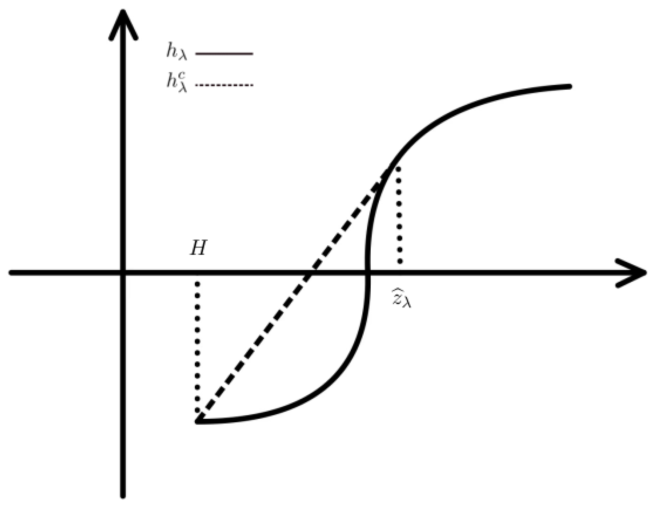
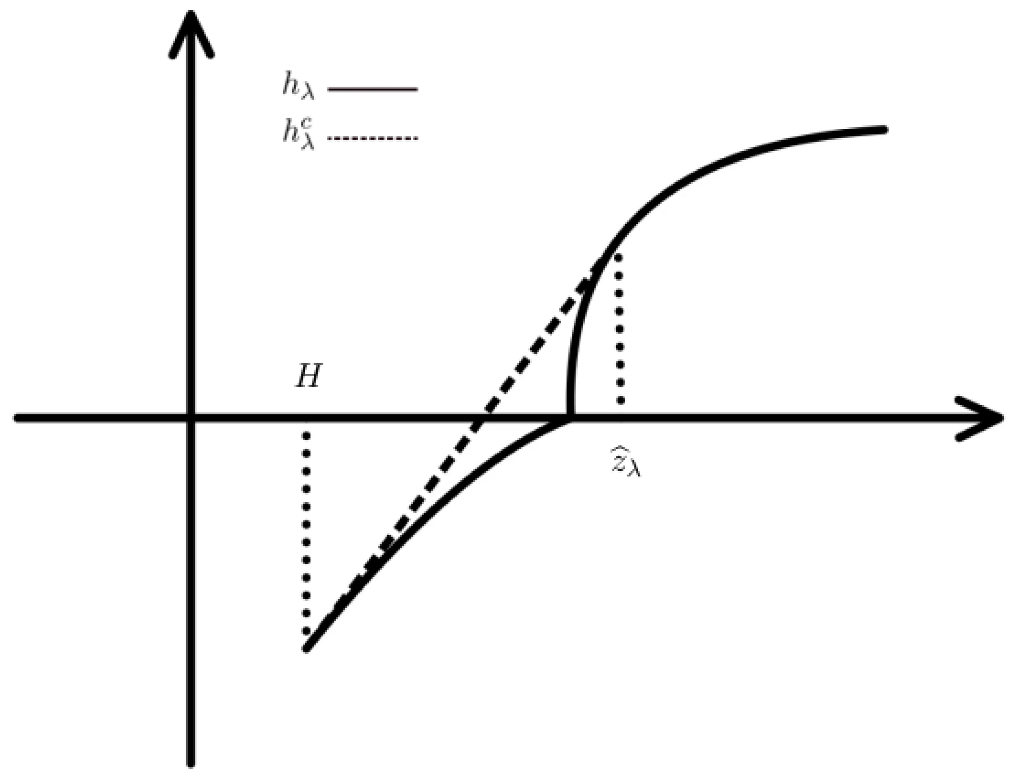
The following two results are useful in deriving the concave envelope of $h_{\lambda }$.

Lemma 3.

For $0<{\gamma }_1<1$, ${\gamma }_2>0$, there exists a unique root ${\hat{z}}_{\lambda }\in ({\displaystyle \frac{{\overline{\theta }}^{*}}{1-\alpha }},\infty )$ to the following equation:

$${((1-\alpha )x-{\overline{\theta }}^{*})}^{{\gamma }_1}-\lambda (1-\alpha ){\gamma }_1{((1-\alpha )x-{\overline{\theta }}^{*})}^{{\gamma }_1-1}(x-H)+\lambda {({\overline{\theta }}^{*}-(1-\alpha )H)}^{{\gamma }_2}=0.$$

(21)

Proof. 

See Appendix A. □

Lemma 4.

We let ${\hat{z}}_{\lambda }$ be given by (21). For $0<{\gamma }_1<1$, ${\gamma }_2>1$, if ${\tilde{k}}_H\left(\lambda \right)>k_{{\hat{z}}_{\lambda }}$, then there exists a unique pair $({\tilde{z}}_{1\lambda },{\tilde{z}}_{2\lambda })$ with $H<{\tilde{z}}_{1\lambda }<{\displaystyle \frac{{\overline{\theta }}^{*}}{1-\alpha }}<{\tilde{z}}_{2\lambda }$ satisfying

$$\begin{array}{ccc}\hfill {\displaystyle \frac{{((1-\alpha ){\tilde{z}}_{2\lambda }-{\overline{\theta }}^{*})}^{{\gamma }_1}-\lambda {({\overline{\theta }}^{*}-(1-\alpha ){\tilde{z}}_{1\lambda })}^{{\gamma }_2}}{{\tilde{z}}_{2\lambda }-{\tilde{z}}_{1\lambda }}}& =& (1-\alpha ){\gamma }_1{((1-\alpha ){\tilde{z}}_{2\lambda }-{\overline{\theta }}^{*})}^{{\gamma }_1-1}\hfill \\ & =& \lambda (1-\alpha ){\gamma }_2{({\overline{\theta }}^{*}-(1-\alpha ){\tilde{z}}_{1\lambda })}^{{\gamma }_2-1}.\hfill \end{array}$$

(22)

Proof. 

See Appendix A. □

Proposition 3.

We let ${\hat{z}}_{\lambda }$ be determined by Equation (21). Then, the concave envelope of $h_{\lambda }$ and the optimal solution to Problem (19) are given as follows:

(a) 

For $0<{\gamma }_1<1,0<{\gamma }_2\le 1$,

$$h_{\lambda }^c\left(x\right)=\left\{\begin{array}{cc}{k}_{{\hat{z}}_{\lambda }}x-\lambda {({\overline{\theta }}^{*}-(1-\alpha )H)}^{{\gamma }_2}-k_{{\hat{z}}_{\lambda }}H,\hfill & H\le x<{\hat{z}}_{\lambda },\hfill \\ h_{\lambda }\left(x\right),\hfill & x\ge {\hat{z}}_{\lambda },\hfill \end{array}\right.$$

(23)

and

$$x_{\lambda }^{*}\left(y\right)=\left\{\begin{array}{cc}{\left({\displaystyle \frac{y}{(1-\alpha ){\gamma }_1}}\right)}^{{\displaystyle \frac{1}{{\gamma }_1-1}}}·{\displaystyle \frac{1}{(1-\alpha )}}+{\displaystyle \frac{{\overline{\theta }}^{*}}{1-\alpha }},\hfill & 0<y\le k_{{\hat{z}}_{\lambda }},\hfill \\ H,\hfill & y>k_{{\hat{z}}_{\lambda }}.\hfill \end{array}\right.$$

(24)

(b) 

For $0<{\gamma }_1<1,{\gamma }_2>1$,

(b1) 

if ${\tilde{k}}_H\left(\lambda \right)\le k_{{\hat{z}}_{\lambda }}$, then the concave envelope of $h_{\lambda }$ and the optimal solution to Problem (19) are given by (23) and (24), respectively;

(b2) 

if ${\tilde{k}}_H\left(\lambda \right)>k_{{\hat{z}}_{\lambda }}$, then the concave envelope of $h_{\lambda }$ is given by

$$h_{\lambda }^c\left(x\right)=\left\{\begin{array}{cc}{h}_{\lambda }\left(x\right),\hfill & H\le x\le {\tilde{z}}_{1\lambda },\hfill \\ k_{{\tilde{z}}_{2\lambda }}(x-{\tilde{z}}_{2\lambda })+h_{\lambda }\left({\tilde{z}}_{2\lambda }\right),\hfill & {\tilde{z}}_{1\lambda }<x<{\tilde{z}}_{2\lambda },\hfill \\ h_{\lambda }\left(x\right),\hfill & x\ge {\tilde{z}}_{2\lambda },\hfill \end{array}\right.$$

(25)

and

$$x_{\lambda }^{*}\left(y\right)=\left\{\begin{array}{cc}{\left({\displaystyle \frac{y}{(1-\alpha ){\gamma }_1}}\right)}^{{\displaystyle \frac{1}{{\gamma }_1-1}}}·{\displaystyle \frac{1}{(1-\alpha )}}+{\displaystyle \frac{{\overline{\theta }}^{*}}{1-\alpha }},\hfill & 0<y\le k_{{\tilde{z}}_{2\lambda }}\hfill \\ {\displaystyle \frac{{\overline{\theta }}^{*}}{1-\alpha }}-{\left({\displaystyle \frac{y}{(1-\alpha )\lambda {\gamma }_2}}\right)}^{{\displaystyle \frac{1}{{\gamma }_2-1}}}·{\displaystyle \frac{1}{(1-\alpha )}},\hfill & k_{{\tilde{z}}_{2\lambda }}<y\le {\tilde{k}}_H\left(\lambda \right)\hfill \\ H,\hfill & y>{\tilde{k}}_H\left(\lambda \right),\hfill \end{array}\right.$$

(26)

where the pair $({\tilde{z}}_{1\lambda },{\tilde{z}}_{2\lambda })$ is determined by (22).

Proof. 

See Appendix A. □

It remains to prove that there exists a positive constant ${\beta }^{*}$ satisfying the budget constraint $\mathbb{E}\left[H^{\hat{\nu }}\left(T\right)x_{\lambda }^{*}\left({\beta }^{*}{H}^{\hat{\nu }}\left(T\right)\right)\right]=x_0.$

Proposition 4.

We suppose that $H{e}^{-rT}\le x_0<{\displaystyle \frac{e^{-rT}{\overline{\theta }}^{*}}{1-\alpha }}$. For each $\lambda \ge 0$, there exists a unique constant ${\beta }^{*}\left(\lambda \right)>0$ such that $Z_{\lambda }^{*}:=Z_{\lambda ,{\beta }^{*}\left(\lambda \right)}^{*}\equiv x_{\lambda }^{*}\left({\beta }^{*}\left(\lambda \right)H^{\hat{\nu }}\left(T\right)\right)$ satisfies $\mathbb{E}\left[H^{\hat{\nu }}\left(T\right)Z_{\lambda ,{\beta }^{*}\left(\lambda \right)}^{*}\right]=x_0$, where $x_{\lambda }^{*}$ is given in (24) and (26).

Proof. 

See Appendix A. □

As such, based on Theorems 1 and 2, Proposition 2, Lemma 2, and Proposition 4, we can obtain the optimal solution to the original optimization Problem (7) by the following procedures:

Algorithm for finding the optimal terminal wealth to Problem (7) and Lagrange multipliers.

• Step 1. Use Proposition 3 to obtain the optimal solution $x_{\lambda }^{*}$ to the non-random Problem (19);
• Step 2. For each $\lambda \ge 0$, find the corresponding ${\beta }^{*}\left(\lambda \right)$ by solving $\mathbb{E}[H^{\hat{\nu }}\left(T\right)x_{\lambda }^{*}({\beta }^{*}\left(\lambda \right)$$H^{\hat{\nu }}\left(T\right)\left)\right]=x_0$ and set $Z_{\lambda }^{*}=x_{\lambda }^{*}\left({\beta }^{*}\left(\lambda \right)H^{\hat{\nu }}\left(T\right)\right)$;
• Step 3. Solve (14) to obtain the optimal ${\lambda }^{*}$ and obtain the corresponding optimal solution $Z_{{\lambda }^{*}}^{*}$ to Problem (7).

In what follows, we follow the above steps to derive the optimal solution. For each $\lambda \ge 0$, set

$$Z_{\lambda }^{*}:=Z_{\lambda ,{\beta }^{*}\left(\lambda \right)}^{*}\equiv x_{\lambda }^{*}\left({\beta }^{*}\left(\lambda \right)H^{\hat{\nu }}\left(T\right)\right),$$

(27)

where $x_{\lambda }^{*}(.)$ is given by (24) and (26), ${\beta }^{*}\left(\lambda \right)$ is determined by Eq. $\mathbb{E}\left[H^{\hat{\nu }}\left(T\right)Z_{\lambda ,{\beta }^{*}\left(\lambda \right)}^{*}\right]=x_0.$

To derive ${\lambda }^{*}$ from (14), we define

$$f_1\left(\lambda \right):=\mathbb{E}\left\{U\left[{((1-\alpha )Z_{\lambda }^{*}-{\overline{\theta }}^{*})}_{+}\right]\right\},$$

(28)

and

$$f_2\left(\lambda \right):=\mathbb{E}\left\{D\left[{({\overline{\theta }}^{*}-(1-\alpha )Z_{\lambda }^{*})}_{+}\right]\right]\}.$$

(29)

Based on Proposition 3, we can obtain the explicit expressions for $f_1$ and $f_2$ as follows:

To simplify notations and avoid repetitions, for any $\beta >0,\gamma >0,$ we define

$$\left\{\begin{array}{c}{d}_{1,t}\left(\beta \right):={\displaystyle \frac{ln\beta -ln{H}^{\hat{\nu }}\left(t\right)+\left(r-\frac{1}{2}{\parallel \hat{\xi }\parallel }^2\right)(T-t)}{\parallel \hat{\xi }\parallel \sqrt{T-t}}},\hfill \\ \\ d_{2,t}(\beta ;\gamma ):=d_{1,t}\left(\beta \right)+{\displaystyle \frac{\parallel \hat{\xi }\parallel \sqrt{T-t}}{1-\gamma }},\hfill \\ \\ K(\beta ;\gamma ):=\varphi \left[d_{1,t}\left(\beta \right)\right]\left(1+{\displaystyle \frac{\parallel \hat{\xi }\parallel \sqrt{T-t}}{1-\gamma }}{\displaystyle \frac{\Phi \left[d_{2,t}(\beta ;\gamma )\right]}{\varphi \left[d_{2,t}(\beta ;\gamma )\right]}}\right),\hfill \end{array}\right.$$

(30)

where $\Phi$ and $\varphi$ denote the standard normal distribution function and its density function, respectively.

Proposition 5.

For $0<{\gamma }_1<1,0<{\gamma }_2\le 1$,

$$\left\{\begin{array}{c}{f}_1\left(\lambda \right)={\left({\displaystyle \frac{1}{1-\alpha }}\right)}^{{\displaystyle \frac{{\gamma }_1}{{\gamma }_1-1}}}·e^{-rT}·{\beta }^{*}\left(\lambda \right)·{\gamma }_1^{{\displaystyle \frac{{\gamma }_1}{1-{\gamma }_1}}}{\displaystyle \frac{\varphi \left[d_{1,0}\left(\frac{1}{{\beta }^{*}\left(\lambda \right)}\right)\right]}{\varphi \left[d_{2,0}\left(\frac{1}{{\beta }^{*}\left(\lambda \right)};{\gamma }_1\right)\right]}}\Phi \left[d_{2,0}\left({\displaystyle \frac{k_{{\hat{z}}_{\lambda }}}{{\beta }^{*}\left(\lambda \right)}};{\gamma }_1\right)\right],\hfill \\ f_2\left(\lambda \right)={({\overline{\theta }}^{*}-(1-\alpha )H)}^{{\gamma }_2}\left\{1-\Phi \left[d_{1,0}\left({\displaystyle \frac{k_{{\hat{z}}_{\lambda }}}{{\beta }^{*}\left(\lambda \right)}}\right)+\parallel \hat{\xi }\parallel \sqrt{T}\right]\right\}.\hfill \end{array}\right.$$

(31)

Proof. 

See Appendix A. □

Proposition 6.

For $0<{\gamma }_1<1,{\gamma }_2>1$, we have

(b1) 

if ${\tilde{k}}_H\left(\lambda \right)\le k_{{\hat{z}}_{\lambda }}$, then $f_1\left(\lambda \right)$ and $f_2\left(\lambda \right)$ are given by (31);

(b2) 

if ${\tilde{k}}_H\left(\lambda \right)>k_{{\hat{z}}_{\lambda }}$, then

$$\left\{\begin{array}{cc}{f}_1\left(\lambda \right)\hfill & ={\left({\displaystyle \frac{1}{1-\alpha }}\right)}^{{\displaystyle \frac{{\gamma }_1}{{\gamma }_1-1}}}·e^{-rT}·{\beta }^{*}\left(\lambda \right)·{\gamma }_1^{{\displaystyle \frac{{\gamma }_1}{1-{\gamma }_1}}}{\displaystyle \frac{\varphi \left[d_{1,0}\left(\frac{1}{{\beta }^{*}\left(\lambda \right)}\right)\right]}{\varphi \left[d_{2,0}\left(\frac{1}{{\beta }^{*}\left(\lambda \right)};{\gamma }_1\right)\right]}}\Phi \left[d_{2,0}\left({\displaystyle \frac{k_{{\tilde{z}}_{2\lambda }}}{{\beta }^{*}\left(\lambda \right)}};{\gamma }_1\right)\right],\hfill \\ f_2\left(\lambda \right)\hfill & ={\left({\displaystyle \frac{1}{1-\alpha }}\right)}^{{\displaystyle \frac{{\gamma }_2}{{\gamma }_2-1}}}·e^{-rT}·{\beta }^{*}\left(\lambda \right)·{\left(\lambda {\gamma }_2\right)}^{{\displaystyle \frac{{\gamma }_2}{1-{\gamma }_2}}}{\displaystyle \frac{\varphi \left[d_{1,0}\left(\frac{1}{{\beta }^{*}\left(\lambda \right)}\right)\right]}{\varphi \left[d_{2,0}\left(\frac{1}{{\beta }^{*}\left(\lambda \right)};{\gamma }_2\right)\right]}}\hfill \\ \hfill & \times \left\{\Phi \left[d_{2,0}\left({\displaystyle \frac{\lambda (1-\alpha ){\gamma }_2·{({\overline{\theta }}^{*}-(1-\alpha )H)}^{{\gamma }_2-1}}{{\beta }^{*}\left(\lambda \right)}};{\gamma }_2\right)\right]-\Phi \left[d_{2,0}\left({\displaystyle \frac{k_{{\tilde{z}}_{2\lambda }}}{{\beta }^{*}\left(\lambda \right)}};{\gamma }_2\right)\right]\right\}\hfill \\ \hfill & +{({\overline{\theta }}^{*}-(1-\alpha )H)}^{*{\gamma }_2}\left\{1-\Phi \left[d_{1,0}\left({\displaystyle \frac{\lambda (1-\alpha ){\gamma }_2·{({\overline{\theta }}^{*}-(1-\alpha )H)}^{{\gamma }_2-1}}{{\beta }^{*}\left(\lambda \right)}}\right)+\parallel \hat{\xi }\parallel \sqrt{T}\right]\right\}.\hfill \end{array}\right.$$

(32)

Proof. 

See Appendix A. □

Once the closed-form expressions for $f_1$ and $f_2$ are derived, we can determine the optimal Lagrange multiplier ${\lambda }^{*}>0$ satisfying

$$f_1\left({\lambda }^{*}\right)-{\lambda }^{*}{f}_2\left({\lambda }^{*}\right)=0.$$

(33)

Given ${\lambda }^{*}>0$, we present the optimal solution for the portfolio optimization Problem (8) in the following results.

Proposition 7.

We assume that $H{e}^{-rT}\le x_0<{\displaystyle \frac{e^{-rT}{\overline{\theta }}^{*}}{1-\alpha }}$. Then, for $0<{\gamma }_1<1,0<{\gamma }_2\le 1$, the optimal terminal wealth, the optimal portfolio value at time $t(0\le t<T)$, and the optimal trading strategy are given as follows:

The optimal terminal wealth is

$$X^{*}\left(T\right)=\left[{({\displaystyle \frac{{\beta }^{*}\left({\lambda }^{*}\right)H^{\hat{\nu }}\left(T\right)}{(1-\alpha ){\gamma }_1}})}^{{\displaystyle \frac{1}{{\gamma }_1-1}}}·{\displaystyle \frac{1}{(1-\alpha )}}+{\displaystyle \frac{{\overline{\theta }}^{*}}{1-\alpha }}\right]{\mathbf{1}}_{\{H^{\hat{\nu }}\left(T\right)\le {\displaystyle \frac{k_{{\hat{z}}_{{\lambda }^{*}}}}{{\beta }^{*}\left({\lambda }^{*}\right)}}\}}+H{\mathbf{1}}_{\{H^{\hat{\nu }}\left(T\right)>{\displaystyle \frac{k_{{\hat{z}}_{{\lambda }^{*}}}}{{\beta }^{*}\left({\lambda }^{*}\right)}}\}},$$

(34)

where ${\lambda }^{*}>0$ is determined by (33) with $f_1$ and $f_2$ given by (31), $k_{{\hat{z}}_{{\lambda }^{*}}}$ is defined by (20), ${\hat{z}}_{{\lambda }^{*}}$ is the solution to Equation (21) with $\lambda ={\lambda }^{*}$.

The optimal portfolio value at time $t(0\le t<T)$ is given by

$$\left\{\begin{array}{c}{X}^{*}\left(t\right)={\mathrm{e}}^{-r(T-t)}(A_1+A_2+A_3),\hfill \\ A_1={\left({\displaystyle \frac{1}{1-\alpha }}\right)}^{{\displaystyle \frac{{\gamma }_1}{{\gamma }_1-1}}}{\left({\displaystyle \frac{k_{{\hat{z}}_{{\lambda }^{*}}}}{{\gamma }_1}}\right)}^{{\displaystyle \frac{1}{{\gamma }_1-1}}}{\displaystyle \frac{\varphi \left[d_{1,t}\left(\frac{k_{{\hat{z}}_{{\lambda }^{*}}}}{{\beta }^{*}\left({\lambda }^{*}\right)}\right)\right]}{\varphi \left[d_{2,t}(\frac{k_{{\hat{z}}_{{\lambda }^{*}}}}{{\beta }^{*}\left({\lambda }^{*}\right)};{\gamma }_1)\right]}}\Phi \left[d_{2,t}({\displaystyle \frac{k_{{\hat{z}}_{{\lambda }^{*}}}}{{\beta }^{*}\left({\lambda }^{*}\right)}};{\gamma }_1)\right],\hfill \\ A_2={\displaystyle \frac{{\overline{\theta }}^{*}}{1-\alpha }}\Phi \left[d_{1,t}\left({\displaystyle \frac{k_{{\hat{z}}_{{\lambda }^{*}}}}{{\beta }^{*}\left({\lambda }^{*}\right)}}\right)\right]\hfill \\ A_3=H(1-\Phi \left[d_{1,t}\left({\displaystyle \frac{k_{{\hat{z}}_{{\lambda }^{*}}}}{{\beta }^{*}\left({\lambda }^{*}\right)}}\right)\right]).\hfill \end{array}\right.$$

(35)

The optimal portfolio invested in the risky asset at time $t(0\le t<T)$ is as follows:

$$\left\{\begin{array}{c}{{\pi }^{*}}^{\top }\left(t\right)={\displaystyle \frac{e^{-r(T-t)}}{\parallel \hat{\xi }\parallel X_t^{*}\sqrt{T-t}}}{\hat{\xi }}^{\top }{\sigma }^{-1}(a_1+a_2-a_3),\hfill \\ a_1={\left({\displaystyle \frac{1}{1-\alpha }}\right)}^{{\displaystyle \frac{{\gamma }_1}{{\gamma }_1-1}}}·{\left({\displaystyle \frac{k_{{\hat{z}}_{{\lambda }^{*}}}}{{\gamma }_1}}\right)}^{{\displaystyle \frac{1}{{\gamma }_1-1}}}K\left({\displaystyle \frac{k_{{\hat{z}}_{{\lambda }^{*}}}}{{\beta }^{*}\left({\lambda }^{*}\right)}};{\gamma }_1\right),\hfill \\ a_2={\displaystyle \frac{{\overline{\theta }}^{*}}{1-\alpha }}\varphi \left[d_{1,t}\left({\displaystyle \frac{k_{{\hat{z}}_{{\lambda }^{*}}}}{{\beta }^{*}\left({\lambda }^{*}\right)}}\right)\right]\hfill \\ a_3=H\varphi \left[d_{1,t}\left({\displaystyle \frac{k_{{\hat{z}}_{{\lambda }^{*}}}}{{\beta }^{*}\left({\lambda }^{*}\right)}}\right)\right].\hfill \end{array}\right.$$

(36)

Proof. 

See Appendix A. □

Proposition 8.

We assume that $H{e}^{-rT}\le x_0<{\displaystyle \frac{e^{-rT}{\overline{\theta }}^{*}}{1-\alpha }}$. For $0<{\gamma }_1<1,{\gamma }_2>1$,

(b1)

if ${\tilde{k}}_H\left({\lambda }^{*}\right)\le k_{{\hat{z}}_{{\lambda }^{*}}},$ then the optimal terminal wealth, the optimal portfolio value at time $t(0\le t<T)$, and the optimal trading strategy are given by (34), (35) and (36), respectively;

(b2)

if ${\tilde{k}}_H\left({\lambda }^{*}\right)>k_{{\hat{z}}_{{\lambda }^{*}}},$ then the optimal terminal wealth, the optimal portfolio value at time $t(0\le t<T)$, and the optimal trading strategy are as follows:

The optimal terminal wealth is given by

$$\begin{array}{cc}\hfill X^{*}\left(T\right)=& \left[{\left({\displaystyle \frac{1}{1-\alpha }}\right)}^{{\displaystyle \frac{{\gamma }_1}{{\gamma }_1-1}}}·{\left({\displaystyle \frac{{\beta }^{*}\left({\lambda }^{*}\right)H^{\hat{\nu }}\left(T\right)}{{\gamma }_1}}\right)}^{{\displaystyle \frac{1}{{\gamma }_1-1}}}+{\displaystyle \frac{{\overline{\theta }}^{*}}{1-\alpha }}\right]{\mathbf{1}}_{\{H^{\hat{\nu }}\left(T\right)\le {\displaystyle \frac{k_{{\tilde{z}}_{2{\lambda }^{*}}}}{{\beta }^{*}\left({\lambda }^{*}\right)}}\}}\hfill \\ \hfill & +\left[{\displaystyle \frac{{\overline{\theta }}^{*}}{1-\alpha }}-{\left({\displaystyle \frac{1}{1-\alpha }}\right)}^{{\displaystyle \frac{{\gamma }_2}{{\gamma }_2-1}}}·{\left({\displaystyle \frac{{\beta }^{*}\left({\lambda }^{*}\right)H^{\hat{\nu }}\left(T\right)}{{\lambda }^{*}{\gamma }_2}}\right)}^{{\displaystyle \frac{1}{{\gamma }_2-1}}}\right]{\mathbf{1}}_{\{{\displaystyle \frac{k_{{\tilde{z}}_{2{\lambda }^{*}}}}{{\beta }^{*}\left({\lambda }^{*}\right)}}<H^{\hat{\nu }}\left(T\right)\le {\displaystyle \frac{{\tilde{k}}_H\left({\lambda }^{*}\right)}{{\beta }^{*}\left({\lambda }^{*}\right)}}\}}\hfill \\ \hfill & +H{\mathbf{1}}_{\{H^{\hat{\nu }}\left(T\right)>{\displaystyle \frac{{\tilde{k}}_H\left({\lambda }^{*}\right)}{{\beta }^{*}\left({\lambda }^{*}\right)}}\}},\hfill \end{array}$$

(37)

where ${\lambda }^{*}>0$ is determined by (33) with $f_1$ and $f_2$ given by (32), ${\tilde{k}}_H\left({\lambda }^{*}\right)$ is defined in (20).

The optimal portfolio value at time $t(0\le t<T)$ is as follows:

$$\left\{\begin{array}{c}{X}^{*}\left(t\right)=e^{-r(T-t)}(B_1+B_2-B_3+B_4),\hfill \\ B_1={\left({\displaystyle \frac{1}{1-\alpha }}\right)}^{{\displaystyle \frac{{\gamma }_1}{{\gamma }_1-1}}}·{\left({\displaystyle \frac{k_{{\tilde{z}}_{2{\lambda }^{*}}}}{{\gamma }_1}}\right)}^{{\displaystyle \frac{1}{{\gamma }_1-1}}}{\displaystyle \frac{\varphi \left[d_{1,t}\left(\frac{k_{{\tilde{z}}_{2{\lambda }^{*}}}}{{\beta }^{*}\left({\lambda }^{*}\right)}\right)\right]}{\varphi \left[d_{2,t}\left(\frac{k_{{\tilde{z}}_{2{\lambda }^{*}}}}{{\beta }^{*}\left({\lambda }^{*}\right)};{\gamma }_1\right)\right]}}·\Phi \left[d_{2,t}\left({\displaystyle \frac{k_{{\tilde{z}}_{2{\lambda }^{*}}}}{{\beta }^{*}\left({\lambda }^{*}\right)}};{\gamma }_1\right)\right],\hfill \\ B_2={\displaystyle \frac{{\overline{\theta }}^{*}}{1-\alpha }}\Phi \left[d_{1,t}\left({\displaystyle \frac{{\tilde{k}}_H\left({\lambda }^{*}\right)}{{\beta }^{*}\left({\lambda }^{*}\right)}}\right)\right],\hfill \\ B_3={\left({\displaystyle \frac{1}{1-\alpha }}\right)}^{{\displaystyle \frac{{\gamma }_2}{{\gamma }_2-1}}}·{\left({\lambda }^{*}{\gamma }_2\right)}^{{\displaystyle \frac{1}{1-{\gamma }_2}}}{\displaystyle \frac{\varphi \left[d_{1,t}\left(\frac{1}{{\beta }^{*}\left({\lambda }^{*}\right)}\right)\right]}{\varphi \left[d_{2,t}\left(\frac{1}{{\beta }^{*}\left({\lambda }^{*}\right)};{\gamma }_2\right)\right]}}\hfill \\ \times \left\{\Phi \left[d_{2,t}\left({\displaystyle \frac{{\tilde{k}}_H\left({\lambda }^{*}\right)}{{\beta }^{*}\left({\lambda }^{*}\right)}};{\gamma }_2\right)\right]-\Phi \left[d_{2,t}\left({\displaystyle \frac{k_{{\tilde{z}}_{2\lambda }}}{{\beta }^{*}\left({\lambda }^{*}\right)}};{\gamma }_2\right)\right]\right\}\hfill \\ B_4=H(1-\Phi \left[d_{1,t}\left({\displaystyle \frac{{\tilde{k}}_H\left({\lambda }^{*}\right)}{{\beta }^{*}\left({\lambda }^{*}\right)}}\right)\right]).\hfill \end{array}\right.$$

(38)

The optimal portfolio invested in the risky asset at time $t(0\le t<T)$ is given by

$$\left\{\begin{array}{c}{{\pi }^{*}}^{\top }\left(t\right)={\displaystyle \frac{e^{-r(T-t)}}{\parallel \hat{\xi }\parallel X_t^{*}\sqrt{T-t}}}{\hat{\xi }}^{\top }{\sigma }^{-1}(b_1+b_2+b_3-b_4),\hfill \\ b_1={\left({\displaystyle \frac{1}{1-\alpha }}\right)}^{{\displaystyle \frac{{\gamma }_1}{{\gamma }_1-1}}}·{\left({\displaystyle \frac{k_{{\tilde{z}}_{2{\lambda }^{*}}}}{{\gamma }_1}}\right)}^{{\displaystyle \frac{1}{{\gamma }_{1-1}}}}K\left({\displaystyle \frac{k_{{\tilde{z}}_{2{\lambda }^{*}}}}{{\beta }^{*}\left({\lambda }^{*}\right)}};{\gamma }_1\right),\hfill \\ b_2={\displaystyle \frac{{\overline{\theta }}^{*}}{1-\alpha }}\varphi \left[d_{1,t}\left({\displaystyle \frac{{\tilde{k}}_H\left({\lambda }^{*}\right)}{{\beta }^{*}\left({\lambda }^{*}\right)}}\right)\right],\hfill \\ b_3=({\displaystyle \frac{{\overline{\theta }}^{*}}{1-\alpha }}-H)\times K\left({\displaystyle \frac{{\tilde{k}}_H\left({\lambda }^{*}\right)}{{\beta }^{*}\left({\lambda }^{*}\right)}};{\gamma }_2\right)-{\left({\displaystyle \frac{1}{1-\alpha }}\right)}^{{\displaystyle \frac{{\gamma }_2}{{\gamma }_2-1}}}·{\left({\displaystyle \frac{k_{{\tilde{z}}_{2{\lambda }^{*}}}}{{\lambda }^{*}{\gamma }_2}}\right)}^{{\displaystyle \frac{1}{{\gamma }_2-1}}}K\left({\displaystyle \frac{k_{{\tilde{z}}_{2{\lambda }^{*}}}}{{\beta }^{*}\left({\lambda }^{*}\right)}};{\gamma }_2\right)\hfill \\ b_4=H\varphi \left[d_{1,t}\left({\displaystyle \frac{{\tilde{k}}_H\left({\lambda }^{*}\right)}{{\beta }^{*}\left({\lambda }^{*}\right)}}\right)\right].\hfill \end{array}\right.$$

(39)

Proof. 

Since the proof is similar to that of Proposition 7, we omit the proof here. □

Remark 4.

From Proposition 7, we can see that for $0<{\gamma }_2\le 1,$ the manager is loss averse towards losses and the optimal terminal wealth $X^{*}\left(T\right)$ takes a two-region form. When the state price density $H^{\hat{\nu }}\left(T\right)$ is relatively low, $X^{*}\left(T\right)$ is similar to the smooth utility; when $H^{\hat{\nu }}\left(T\right)$ increases above a critical value of the price density, $X^{*}\left(T\right)$ drops to H since the loss aversion states a risk-seeking preference in the loss domain.

From Proposition 8, we can observe that for ${\gamma }_2>1,$ the manager is risk-averse towards losses and the optimal terminal wealth $X^{*}\left(T\right)$ takes a two- or three-region form. Comparing with the case that $0<{\gamma }_2\le 1,$ risk aversion towards losses may lead to an increase in the optimal terminal wealth for ${\gamma }_2>1,$ by letting $X^{*}\left(T\right)={\displaystyle \frac{{\overline{\theta }}^{*}}{1-\alpha }}-{\left({\displaystyle \frac{1}{1-\alpha }}\right)}^{{\displaystyle \frac{{\gamma }_2}{{\gamma }_2-1}}}·{\left({\displaystyle \frac{{\beta }^{*}\left({\lambda }^{*}\right)H^{\hat{\nu }}\left(T\right)}{{\lambda }^{*}{\gamma }_2}}\right)}^{{\displaystyle \frac{1}{{\gamma }_2-1}}}$ in the region ${\displaystyle \frac{k_{{\tilde{z}}_{2{\lambda }^{*}}}}{{\beta }^{*}\left({\lambda }^{*}\right)}}<H^{\hat{\nu }}\left(T\right)\le {\displaystyle \frac{{\tilde{k}}_H\left({\lambda }^{*}\right)}{{\beta }^{*}\left({\lambda }^{*}\right)}}$ if ${\tilde{k}}_H\left({\lambda }^{*}\right)>k_{{\hat{z}}_{{\lambda }^{*}}}.$

For each case, the the optimal terminal wealth $X^{*}\left(T\right)$ ends with the protection level $H,$ which implies the PI constraint can protect the investor’s benefits by keeping $X^{*}\left(T\right)$ above the protection level H.

4. Numerical Analysis

In this section, we aim to carry out some numerical calculations to investigate the impacts of the model parameters on the optimal solution. Furthermore, we compare the optimal investment behavior under our model with that under the model in [17].

4.1. Sensitivity Analysis

We assume that the financial market consists of three tradable assets, whose price processes are modelled by (1)–(2) with $n=2$. We let

$$\sigma =\left(\begin{array}{cc}{\sigma }_1& 0\\ \rho {\sigma }_2& \sqrt{1-{\rho }^2}{\sigma }_2\end{array}\right)$$

Then $\xi ={({\vartheta }_1,{\displaystyle \frac{{\vartheta }_2-\rho {\vartheta }_1}{\sqrt{1-{\rho }^2}}})}^{\top },$ where ${\vartheta }_1={\displaystyle \frac{{\mu }_1-r}{{\sigma }_1}}>0,{\vartheta }_2={\displaystyle \frac{{\mu }_2-r}{{\sigma }_2}}>0$ are the Sharpe ratios of the two risky assets, respectively. We let $K={[0,\infty )}^2,$ which means short-selling is not allowed. The positive polar cone of K is given by $\tilde{K}={[0,\infty )}^2.$ From Proposition 3.14 in [19], we have

$$\begin{array}{c}\hfill \hat{\xi }=\left\{\begin{array}{cc}{\left({\vartheta }_1,{\displaystyle \frac{{\vartheta }_2-\rho {\vartheta }_1}{\sqrt{1-{\rho }^2}}}\right)}^{\top },\hfill & {\vartheta }_2>\rho {\vartheta }_1,{\vartheta }_1>\rho {\vartheta }_2,\hfill \\ {({\vartheta }_1,0)}^{\top },\hfill & \rho {\vartheta }_1\ge {\vartheta }_2,\hfill \\ {(\rho {\vartheta }_2,\sqrt{1-{\rho }^2}{\vartheta }_2)}^{\top },\hfill & \rho {\vartheta }_2\ge {\vartheta }_1.\hfill \end{array}\right.\end{array}$$

Note that when $K={(-\infty ,\infty )}^2,$ we have $\tilde{K}=\left\{{(0,0)}^{\top }\right\}$ and $\hat{\xi }={\left({\vartheta }_1,{\displaystyle \frac{{\vartheta }_2-\rho {\vartheta }_1}{\sqrt{1-{\rho }^2}}}\right)}^{\top }.$

For all numerical computations, the benchmark data used are listed in Table 1.

Table 1. Benchmark data.

${\mathit{x}}_0$	T	r	${\mathit{\mu }}_1$	${\mathit{\mu }}_2$	${\mathit{\sigma }}_1$	${\mathit{\sigma }}_2$	$\mathit{\theta }\left(0\right)$	H	${\mathit{\gamma }}_1$	${\mathit{\gamma }}_2$	$\mathit{\alpha }$	$\mathit{\rho }$
35	40	$0.02$	$0.06$	$0.065$	$0.3$	$0.4$	45	20	$0.4$	$0.2\left(\mathrm{or}1.3\right)$	$0.5$	$0.8$

Figure 1 and Figure 2 show the optimal terminal wealth $X^{*}\left(T\right)$ versus $H^{\hat{\nu }}\left(T\right)$ for different H with ${\gamma }_2=0.2$ and ${\gamma }_2=1.3$, respectively. We see that the optimal terminal wealth $X^{*}\left(T\right)$ with ${\gamma }_2=0.2$ takes a two-region form, while $X^{*}\left(T\right)$ with ${\gamma }_2=1.3$ takes a three-region form, which is consistent with the results in Propositions 3.8 and 3.9. Comparing these two figures, we can observe that in the loss domain for those states with optimal terminal wealth below the benchmark, the manager with ${\gamma }_2=1.3$ may take a conservative allocation strategy to lead to an increase in the optimal terminal wealth of bad economic states, as ${\gamma }_2>1$ implies that the manager is risk-averse towards losses. It is seen from Figure 1 and Figure 2 that the PI constraint requires the manager to keep the optimal terminal wealth above a minimum guarantee H. We can also observe that a higher protection level H is at the expense of the optimal terminal wealth in the good-states region. Furthermore, as H decreases, the bad-states region enlarges while the good-states region shrinks. This is because in order to achieve a higher protection level H, more states are insured against.

Figure 1. $X^{*}\left(T\right)$ versus $H^{\hat{\nu }}\left(T\right)$ for different H with ${\gamma }_2=0.2$.

Figure 2. $X^{*}\left(T\right)$ versus $H^{\hat{\nu }}\left(T\right)$ for different H with ${\gamma }_2=1.3$.

Figure 3 and Figure 4 plot the optimal terminal wealth $X^{*}\left(T\right)$ versus $H^{\hat{\nu }}\left(T\right)$ for different $\alpha$ with ${\gamma }_2=0.2$ and ${\gamma }_2=1.3$, respectively. We can observe that the optimal terminal wealth in the good-states region corresponding to a higher value of $\alpha$ is higher than that corresponding to a lower value of a. When the manager attaches more importance to the optimal wealth in the benchmark, the manager invests more money in the risky assets so that they are more likely to achieve the reference point, leading to a higher optimal terminal wealth in good economic states.

Figure 3. $X^{*}\left(T\right)$ versus $H^{\hat{\nu }}\left(T\right)$ for different $\alpha$ with ${\gamma }_2=0.2$.

Figure 4. $X^{*}\left(T\right)$ versus $H^{\hat{\nu }}\left(T\right)$ for different $\alpha$ with ${\gamma }_2=1.3$.

Figure 5 and Figure 6 present the optimal terminal wealth $X^{*}\left(T\right)$ versus $H^{\hat{\nu }}\left(T\right)$ for different $\theta \left(0\right)$ with ${\gamma }_2=0.2$ and ${\gamma }_2=1.3$, respectively. We can see that the optimal terminal wealth in the good states region corresponding to a higher value of $\theta \left(0\right)$ is higher than that corresponding to a lower value of $\theta \left(0\right)$. From Figure 5 and Figure 6, we can observe that the optimal terminal wealth in good states region increases with $\theta \left(0\right)$. This is due to the fact that as $\theta \left(0\right)$ increases, the manager invests more money in the risky assets to maximize their opportunity to beat the benchmark $\theta \left(T\right)$, which leads to a better optimal terminal performance in the good states region.

Figure 5. $X^{*}\left(T\right)$ versus $H^{\hat{\nu }}\left(T\right)$ for different $\theta \left(0\right)$ with ${\gamma }_2=0.2$.

Figure 6. $X^{*}\left(T\right)$ versus $H^{\hat{\nu }}\left(T\right)$ for different $\theta \left(0\right)$ with ${\gamma }_2=1.3$.

Figure 7 graphs the optimal portfolio at time 0 versus $\theta \left(0\right)$ for different $\rho$ with ${\gamma }_2=1.3$. We can observe that the wealth invested in the first risky asset with $\rho =0.9$ is 0. Note that the parameters for the case $\rho =0.9$ satisfy the condition $\rho {\vartheta }_2\ge {\vartheta }_1$. Therefore, the short-selling constraint leads to $\hat{\xi }={(\rho {\vartheta }_2,\sqrt{1-{\rho }^2}{\vartheta }_2)}^{\top }$ and subsequently ${\pi }_1^{*}\left(t\right)=0.$ However, the parameters for case $\rho =0.8$ satisfy ${\vartheta }_2>\rho {\vartheta }_1,{\vartheta }_1>\rho {\vartheta }_2,$ implying that the optimal control naturally meets the short-selling constraints, i.e., the short-selling constraints are not binding.

Figure 7. ${\pi }^{*}\left(0\right)$ versus $x_0$ for different $\rho$ with ${\gamma }_2=1.3$.

Figure 8 shows the optimal portfolio at time 0 versus H for different ${\gamma }_1$. As shown in Figure 8, the proportions invested in the two risky assets both increase with ${\gamma }_1$. This is due to the fact that ${\gamma }_1$ characterizes the manager’s risk attitude towards gains, and a greater ${\gamma }_1$ means less risk aversion, leading to more investment in risky assets.

Figure 8. ${\pi }^{*}\left(0\right)$ versus H for different ${\gamma }_1$.

Figure 9 plots the optimal portfolio at time 0 versus H for different ${\gamma }_2>1$. We observe from Figure 9 that the proportions invested in the two risky assets both decrease with ${\gamma }_2$. The manager is risk-averse towards losses for ${\gamma }_2>1$. Meanwhile, the manager becomes more risk-averse towards losses for a larger ${\gamma }_2$, Therefore, they decreas investment in risky assets.

Figure 9. ${\pi }^{*}\left(0\right)$ versus H for different ${\gamma }_2$.

Figure 10 graphs the optimal portfolio at time 0 versus H with ${\gamma }_2=0.2$ and ${\gamma }_2=1.3,$ respectively. It is seen from Figure 10 that the proportions invested in the risky assets corresponding to ${\gamma }_2=0.2$ are higher than those corresponding to ${\gamma }_2=1.3.$ The reason is that the manager is risk-averse towards losses for ${\gamma }_2>1$ while they are risk-seeking in the loss domain for $0<{\gamma }_2<1$. Therefore, the manager with $0<{\gamma }_2<1$ invests more in risky assets.

Figure 10. ${\pi }^{*}\left(0\right)$ versus H with ${\gamma }_2=0.2,1.3$.

4.2. Model Comparison

In this subsection, we make some comparisons in the optimal investment behaviors between our model and the model in [17]. Hereafter, we refer to our model and the model in [17] as Model I and Model II, respectively. Since the aim is to compare the impacts of two different stochastic benchmarks on the optimal investment behaviors, we follow [17] to assume that the financial market consists of two tradable securities: A risk-free security and a risky asset and there are no position and PI constraints. The parameters are all borrowed from [17].

We let CSI 500 index be the risky asset and the parameter values are as follows: $r=0.03$, $\mu =0.07,\sigma =0.3$ according to the empirical data on the financial market. We assume ${\gamma }_1={\gamma }_2=\gamma =0.88$ as estimated in [25]. We let $T=5$, $x_0=100$, ${\theta }_0=150$. The weight $\alpha$ is set to be 0.5. Accordingly, under the model in [17], the fixed proportion of wealth invested in risky asset is $\eta =\alpha =0.5.$

Figure 11 and Figure 12 represent the impacts of the stochastic benchmark on ${\pi }^{*}\left(0\right)$ for Models I, II. We can see from them that the optimal portfolio at time 0 corresponding to Model I is much lower than that corresponding to Model II. This observation numerically illustrates that comparing with an updated benchmark according to the wealth process, the manager may take a more aggressive investment strategy when the benchmark is set to be a value-weighted portfolio with a fixed proportion invested in the risky asset.

Figure 11. ${\pi }^{*}\left(0\right)$ versus $\alpha$ for Models I, II.

Figure 12. ${\pi }^{*}\left(0\right)$ versus ${\theta }_0$ for Models I, II.

Figure 11 plots the optimal portfolio at time 0 versus $\alpha$($\eta$ in Model II) for Models I, II. We can observe from Figure 11 that for the updated benchmark according to the wealth process, ${\pi }^{*}\left(0\right)$ is an increasing function of $\alpha$. A higher $\alpha$ implies that the adjustment of the benchmark more relies on the wealth process. In fact, Equation (9) implies that the optimization problem with an updating benchmark can be transformed into an optimization problem with a static benchmark ${\displaystyle \frac{{\overline{\theta }}^{*}}{1-\alpha }}.$ With $\alpha$ increasing, the benchmark ${\displaystyle \frac{{\overline{\theta }}^{*}}{1-\alpha }}$ increases accordingly, leading to a higher proportion of wealth invested in the risky asset. It is seen from Figure 11 that for a value-weighted portfolio benchmark in [17], ${\pi }^{*}\left(0\right)$ also increases with $\alpha$. As explained in [17], the benchmark becomes more aggressive with the proportion of wealth invested in the risky asset increasing, and therefore the manager decreases the tracking error and invests more in the risky asset to attain the benchmark.

Figure 12 graphs the optimal portfolio at time 0 versus ${\theta }_0$ for Models I, II. We can see that for the two Models I, II, ${\pi }^{*}\left(0\right)$ both increase with the initial benchmark ${\theta }_0$ since an increase in the initial benchmark leads the manager to invests more in the risky asset to beat the benchmark.

5. Conclusions

In this paper, we investigate the optimal portfolio selection problem of a fund manager when they base decisions on the performance measure comparison to a stochastic benchmark under a PI and position constraints. By using the linearization method, the Lagrangian method and the concavification technique, we derive the optimal wealth process and the optimal investment strategies. The form for the optimal terminal wealth can take a two- or three-region form. In all cases, the optimal terminal wealth ends up with the minimum guarantee from a certain value of the price density. Numerical results show that if the manager attaches more importance to the change in terminal wealth in the benchmark distinguishing the gains and losses, they allocate more money in the risky asset, resulting in higher optimal terminal wealth of good economic states.