Global Dynamics of a Predator–Prey System with Variation Multiple Pulse Intervention Effects

Abstract

A continuous point of a trajectory for an ordinary differential equation can be viewed as a special impulsive point; i.e., the pulsed proportional change rate and the instantaneous increment for the prey and predator populations can be taken as 0. By considering the variation multiple pulse intervention effects (i.e., several indefinite continuous points are regarded as impulsive points), an impulsive predator–prey model for characterizing chemical and biological control processes at different fixed times is first proposed. Our modeling approach can describe all possible realistic situations, and all of the traditional models are some special cases of our model. Due to the complexity of our modeling approach, it is essential to examine the dynamical properties of the periodic solutions using new methods. For example, we investigate the permanence of the system by constructing two uniform lower impulsive comparison systems, indicating the mathematical (or biological) essence of the permanence of our system; furthermore, the existence and global attractiveness of the pest-present periodic solution is analyzed by constructing an impulsive comparison system for a norm $V\left(t\right)$, which has not been addressed to date. Based on the implicit function theorem, the bifurcation of the pest-present periodic solution of the system is investigated under certain conditions, which is more rigorous than the corresponding traditional proving method. In addition, by employing the variational method, the eigenvalues of the Jacobian matrix at the fixed point corresponding to the pest-free periodic solution are determined, resulting in a sufficient condition for its local stability, and the threshold condition for the global attractiveness of the pest-free periodic solution is provided in terms of an indicator $R_a$. Finally, the sensitivity of indicator $R_a$ and bifurcations with respect to several key parameters are determined through numerical simulations, and then the switch-like transitions among two coexisting attractors show that varying dosages of insecticide applications and the numbers of natural enemies released are crucial.

1. Introduction

Pest control has become an increasingly complex issue over the past two decades. Pests in the natural environment not only negatively impact human well-being but also disrupt food production and spread diseases; in the worst scenarios, they even cause death and serious disasters for plants and other living things on Earth [1]. Experimental evidence has demonstrated that these pests reduce the annual production of some agricultural commodities, e.g., $25\%$ shrinkage in rice, $30\%$ shrinkage in pulses, 5–10% shrinkage in wheat, $20\%$ shrinkage in sugarcane, $35\%$ shrinkage in oil seeds, and $50\%$ shrinkage in cotton [2]. This alarming issue has motivated an urgent demand for controlling the negative impact of pests. The traditional pest control method involves the application of a large variety of single pesticides to crops, which is not favorable for controlling the progress of pest resistance and preserving the quality of the environment. Chemical control by spraying pesticides and the simultaneous deployment of biological control by using natural enemies have been commonly applied in integrated pest management (IPM) systems [3,4].

Various mathematical models have been studied for pest control, including chemical and biological control tactics [5,6,7,8]. Researchers have proposed several state-dependent impulsive predator–prey models with integrated pest management to control crop pests and subsequently explored the properties of the Poincaré map and the existence, uniqueness, and local or global stability of the order-k ($k\ge 1$) periodic solutions of the systems by means of the successor function method and the analog of the Poincaré criterion, respectively [9,10,11,12,13,14,15]. For example, Cheng et al. proposed a state-dependent impulsive predator–prey model with Holling type I and II responses and then investigated the properties of the Poincaré map and the existence, uniqueness, and sufficient conditions for the global stability of the order-1 periodic solutions of the system [16]. Al Basir et al. formulated an impulsive integrated pest management model for characterizing the application processes of biopesticides and chemical pesticides at fixed times, and the stability of the pest-free periodic solution was investigated using the small amplitude perturbation method, which established a threshold time limit for the impulsive release of various controls as well as some valid theoretical conclusions for effective pest management [17].

The classes of predator–prey systems can be generalized as follows [18,19]:

$$\left\{\begin{array}{ccc}\hfill {\displaystyle \frac{dx\left(t\right)}{dt}}& =& ax\left(t\right)\left(1-{\displaystyle \frac{x\left(t\right)}{K}}\right)-\alpha \phi \left(x\left(t\right)\right)y\left(t\right),\hfill \\ \hfill {\displaystyle \frac{dy\left(t\right)}{dt}}& =& -Dy\left(t\right)+\beta \phi \left(x\right(t\left)\right)y\left(t\right),\hfill \end{array}\right.$$

where $x\left(t\right)$ and $y\left(t\right)$ are the densities of the prey and predator populations, respectively, at time t. $a>0$ denotes the intrinsic growth rate of the prey population, $K>0$ represents the carrying capacity of the environment, and $\alpha >0$ is the search efficiency of a predator for prey. $D>0$ is the mortality rate of the predator population, and $\beta >0$ is the biomass conversion. $\phi \left(x\right)$ is the generalized functional response.

Since pesticides are harmful to pests and natural enemies, we can introduce the periodic spraying of pesticides and release predators at different instances [20]; thus, Liu et al. proposed an impulsive system as follows [21]:

$$\left\{\begin{array}{c}\left.\begin{array}{ccc}\hfill {\displaystyle \frac{dx\left(t\right)}{dt}}& =& ax\left(t\right)\left(1-{\displaystyle \frac{x\left(t\right)}{K}}\right)-\alpha \phi \left(x\left(t\right)\right)y\left(t\right),\hfill \\ \hfill {\displaystyle \frac{dy\left(t\right)}{dt}}& =& -Dy\left(t\right)+\beta \phi \left(x\right(t\left)\right)y\left(t\right),\hfill \end{array}\right\}t\ne (n-1)T+lT,t\ne nT,\hfill \\ \left.\begin{array}{ccc}\hfill x\left(t^{+}\right)& =& (1-p_P)x\left(t\right),\hfill \\ \hfill y\left(t^{+}\right)& =& (1-p_N)y\left(t\right),\hfill \end{array}\right\}t=(n-1)T+lT,\hfill \\ \left.\begin{array}{ccc}\hfill x\left(t^{+}\right)& =& x\left(t\right),\hfill \\ \hfill y\left(t^{+}\right)& =& y\left(t\right)+q,\hfill \end{array}\right\}t=nT,\hfill \end{array}\right.$$

(1)

where $0<p_N<p_P<1$ represent the constant fractions of the predator and prey populations that die due to pesticides at time $t=(n-1)T+lT$($l\in (0,1)$), respectively. $q\ge 0$ represents the amount of natural enemies released at time $t=nT$.

For system (1), the frequencies of pesticide spraying and predator release are the same, which is not realistic. Similar to the modeling approach in [22], system (1) can be modified into the following system:

$$\left\{\begin{array}{c}\left.\begin{array}{ccc}\hfill {\displaystyle \frac{dx\left(t\right)}{dt}}& =& ax\left(t\right)\left(1-{\displaystyle \frac{x\left(t\right)}{K}}\right)-\alpha \phi \left(x\left(t\right)\right)y\left(t\right),\hfill \\ \hfill {\displaystyle \frac{dy\left(t\right)}{dt}}& =& -Dy\left(t\right)+\beta \phi \left(x\right(t\left)\right)y\left(t\right),\hfill \end{array}\right\}t\ne {\tau }_n,t\ne {\lambda }_m,\hfill \\ \left.\begin{array}{ccc}\hfill x\left(t^{+}\right)& =& (1-p_P)x\left(t\right),\hfill \\ \hfill y\left(t^{+}\right)& =& (1-p_N)y\left(t\right),\hfill \end{array}\right\}t={\tau }_n,\hfill \\ \left.\begin{array}{ccc}\hfill x\left(t^{+}\right)& =& x\left(t\right),\hfill \\ \hfill y\left(t^{+}\right)& =& y\left(t\right)+q,\hfill \end{array}\right\}t={\lambda }_m,\hfill \end{array}\right.$$

(2)

where ${\tau }_n(n=1,2,\cdots )$ and ${\lambda }_m(m=1,2,\cdots )$ are impulsive point series at which the chemical and biological control strategies are applied, respectively. Zhao et al. investigated the global attractiveness of the trivial periodic solution only for the following two cases [22]:

Case I: $0={\lambda }_0<{\tau }_1<{\tau }_2<\cdots <{\tau }_{k_p}<{\lambda }_1=T_N(>0)$, where $k_p>0$;

Case II: $0={\tau }_0<{\lambda }_1<{\lambda }_2<\cdots <{\lambda }_{k_N}<{\tau }_1=T_P(>0)$, where $k_N>0$.

The above two cases are two special cases of real-world implementations of biological and chemical tactics. Thus, a problem arises naturally: is there a more general approach to characterize this kind of impulsive control strategy?

To solve this problem, it should be noted that a continuous point can be viewed as a special impulsive point. Taking system (2) as an example, if $y\left(t\right)$ is continuous at $t=t_0$, then it follows that $y\left(t_0^{+}\right)=(1-p_N)y\left(t_0\right)$, where $p_N=0$; or $y\left(t_0^{+}\right)=y\left(t_0\right)+q$, where $q=0$. Since the Holling type II functional response is common for most of the functional responses mentioned in [18,19], we can take

$$\phi \left(x\left(t\right)\right)={\displaystyle \frac{x\left(t\right)}{b+x\left(t\right)}},$$

where $b>0$ is the half-saturation constant. Then, a novel impulsive system can be formulated as follows [23]:

$$\left\{\begin{array}{c}\left.\begin{array}{ccc}\hfill {\displaystyle \frac{dy\left(t\right)}{dt}}& =& -Dy\left(t\right)+{\displaystyle \frac{\beta x\left(t\right)y\left(t\right)}{b+x\left(t\right)}},\hfill \\ \hfill {\displaystyle \frac{dx\left(t\right)}{dt}}& =& ax\left(t\right)(1-{\displaystyle \frac{x\left(t\right)}{K}})-{\displaystyle \frac{\alpha x\left(t\right)y\left(t\right)}{b+x\left(t\right)}},\hfill \end{array}\right\}\begin{array}{c}t\notin nT+\left\{0,{\lambda }_1,{\lambda }_2,\dots ,{\lambda }_m\right\}\hfill \\ t\notin nT+\left\{{\tau }_1^{\left(j\right)},{\tau }_2^{\left(j\right)},\dots ,{\tau }_{m_j}^{\left(j\right)}\right\},1\le j\le m+1,\hfill \end{array}\hfill \\ \left.\begin{array}{ccc}\hfill y\left(t^{+}\right)& =& \left(1-p_N^{\left(i\right)}\right)y\left(t\right),\hfill \\ \hfill x\left(t^{+}\right)& =& \left(1-p_P^{\left(i\right)}\right)x\left(t\right),\hfill \end{array}\right\}t=nT+{\lambda }_i,1\le i\le m+1,\hfill \\ \left.\begin{array}{ccc}\hfill y\left(t^{+}\right)& =& \left(1+p_k^{\left(j\right)}\right)y\left(t\right)+q_k^{\left(j\right)},\hfill \\ \hfill x\left(t^{+}\right)& =& x\left(t\right),\hfill \end{array}\right\}t=nT+{\tau }_k^{\left(j\right)},1\le k\le m_j,1\le j\le m+1,\hfill \end{array}\right.$$

(3)

where $\left(p_N^{\left(i\right)},p_P^{\left(i\right)}\right)\in \left\{(0,0),(p_N,p_P)\right\}$, $q_k^{\left(j\right)}\in \left\{0,q\right\}$ and $p_k^{\left(j\right)}\in \left\{0,p_M\right\}$. $p_M\ge 0$ represents the immigration rate of natural enemies [24,25,26]. In addition, $m\in {\mathrm{Z}}_{+}$, and

$$\left\{\begin{array}{c}0={\lambda }_0<{\lambda }_1<{\lambda }_2<\cdots <{\lambda }_m<{\lambda }_{m+1}=T,\hfill \\ {\lambda }_{j-1}<{\tau }_1^{\left(j\right)}<{\tau }_2^{\left(j\right)}<\cdots <{\tau }_{m_j}^{\left(j\right)}<{\lambda }_j,1\le j\le m+1,\hfill \end{array}\right.$$

and

$$\left\{\begin{array}{cc}\left.\begin{array}{ccc}\hfill p_N^{(i+n(m+1\left)\right)}& =& p_N^{\left(i\right)},\hfill \\ \hfill p_P^{(i+n(m+1\left)\right)}& =& p_P^{\left(i\right)},\hfill \end{array}\right\}\hfill & 1\le i\le m+1,\hfill \\ \left.\begin{array}{ccc}\hfill p_k^{(j+n(m+1\left)\right)}& =& p_k^{\left(j\right)},\hfill \\ \hfill q_k^{(j+n(m+1\left)\right)}& =& q_k^{\left(j\right)},\hfill \end{array}\right\}& 1\le k\le m_j,1\le j\le m+1.\end{array}\right.$$

It should be noted that $\left(p_N^{\left(i\right)},p_P^{\left(i\right)}\right)=(0,0)$ indicates that pesticides are not sprayed at time $t=nT+{\lambda }_i$. Similarly, $q_k^{\left(j\right)}=0$ (or $p_k^{\left(j\right)}=0$) means that there are no natural enemy releases (or immigration) at time $t=nT+{\tau }_k^{\left(j\right)}$. Thus, the modeling approach for system (3) can characterize all of the possible practical cases for the implementation of biological and chemical control tactics.

The goal of our study is mainly to investigate the existence and global stability of pest-present periodic solutions. Unlike the techniques used in [21], the permanence of system (3) can be analyzed by constructing two uniform lower impulsive comparison systems, indicating the mathematical (or biological) essence of the permanence of system (3). To date, the global stability of the pest-present periodic solution of system (1) has not been addressed. Based on the permanence of system (3), we can define a norm with respect to the solution of system (3) and then construct an impulsive comparison system for this norm. Similar to the proof of the contraction mapping principle, we can prove the global stability of the pest-present periodic solution. Due to the complexity of the modeling approach of the system (3), the local bifurcation of a pest-present periodic solution cannot be solved by traditional methods [27]. We address this issue by using an implicit function theorem and Taylor’s series of two-variable functions. In addition, the local stability of the pest-free periodic solution is investigated by using the variational method, and the global attractiveness of the pest-free periodic solution is also discussed.

The rest of this article is organized as follows. In Section 2, for convenience, we present some definitions and lemmas. In Section 3, the local stability of the pest-free periodic solution is studied using the variational method; and the bifurcation of a pest-present periodic solution of system (3) is studied by using the implicit function theorem and Taylor’s series of a two-variable function. Several additional technical computations that were used to establish the results presented in Section 3 are discussed in Appendix A, Appendix B, Appendix C and Appendix D. Additionally, the global attractiveness of the pest-free periodic solution is discussed in this section. In Section 4, once the threshold condition is satisfied together with a certain other condition, system (3) is permanent; furthermore, the existence and global attractiveness of the pest-present periodic solution are investigated. Numerical simulations that confirm our theoretical findings are discussed in Section 5. Finally, a discussion of the theoretical and numerical results is provided.

2. Preliminaries

In this section, we introduce some definitions and state some preliminary lemmas that will be useful for establishing our results.

Definition  1

([21]). The system (3) is said to be permanent if there are constants $m,M>0$ (independent of the initial values) and a finite time $T_0$ such that for all solutions $\left(y\right(t),x(t\left)\right)$ with all initial values $(y\left(0^{+}\right),x\left(0^{+}\right))>0$, $m\le y\left(t\right),x\left(t\right)\le M$ holds for all $T\ge T_0$. Here, $T_0$ may depend on the initial values $(y\left(0^{+}\right),x\left(0^{+}\right))$.

Note that $x^{\ast }=K$ is a globally stable equilibrium of the system ${\displaystyle \frac{dx}{dt}}=rx(1-{\displaystyle \frac{x}{K}})$. Then, we have the following lemma:

Lemma 1.

The positive orthant ${\mathbb{R}}_{+}^2$ is an invariant region for the system (3), and for a sufficiently large $t>0$, $x\left(t\right)<K$.

In the following, we assume that $0<x\left(t\right)<K$ for $t\ge 0$.

Consider the following subsystem:

$$\left\{\begin{array}{cccc}\hfill {\displaystyle \frac{dy\left(t\right)}{dt}}& =& \mu y\left(t\right),\hfill & t\notin nT+\left\{0,{\lambda }_1,{\lambda }_2,\cdots ,{\lambda }_m\right\},\hfill \\ \hfill & & & t\notin nT+\left\{{\tau }_1^{\left(j\right)},{\tau }_2^{\left(j\right)},\cdots ,{\tau }_{m_j}^{\left(j\right)}\right\},1\le j\le m+1,\hfill \\ \hfill y\left(t^{+}\right)& =& (1-p_N^{\left(i\right)})y\left(t\right),\hfill & t=nT+{\lambda }_i,1\le i\le m+1,\hfill \\ \hfill y\left(t^{+}\right)& =& (1+p_k^{\left(j\right)})y\left(t\right)+q_k^{\left(j\right)},\hfill & t\in nT+{\tau }_k^{\left(j\right)},1\le k\le m_j,1\le j\le m+1,\hfill \end{array}\right.$$

(4)

where $\mu \ne 0$. Then, we have

$$y(t;\mu )=\left\{\begin{array}{cc}y({\lambda }_{j-1}^{+};\mu )e^{\mu (t-{\lambda }_{j-1})},\hfill & t\in ({\lambda }_{j-1},{\tau }_1^{\left(j\right)}],\hfill \\ y\left({\left({\tau }_{k-1}^{\left(j\right)}\right)}^{+};\mu \right)e^{\mu (t-{\tau }_{k-1}^{\left(j\right)})},\hfill & t\in \left({\tau }_{k-1}^{\left(j\right)},{\tau }_k^{\left(j\right)}\right],\hfill \\ \hfill & k=2,3,\cdots ,m_j,\hfill \\ y\left({\left({\tau }_{m_j}^{\left(j\right)}\right)}^{+};\mu \right)e^{\mu (t-{\tau }_{m_j}^{\left(j\right)})},\hfill & t\in \left({\tau }_{m_j}^{\left(j\right)},{\lambda }_j\right],\hfill \end{array}\right.$$

(5)

for $j=1,2,\cdots ,m+1$, where $y(t;\mu )$ is a solution of (4).

It follows from (4) and (5) that

$$\left\{\begin{array}{ccc}\hfill y\left({\left({\tau }_1^{\left(j\right)}\right)}^{+};\mu \right)& =& (1+p_1^{\left(j\right)})e^{\mu ({\tau }_1^{\left(j\right)}-{\lambda }_{j-1})}y({\lambda }_{j-1}^{+};\mu )+q_1^{\left(j\right)},\hfill \\ \hfill y\left({\left({\tau }_k^{\left(j\right)}\right)}^{+};\mu \right)& =& (1+p_k^{\left(j\right)})e^{\mu ({\tau }_k^{\left(j\right)}-{\tau }_{k-1}^{\left(j\right)})}y\left({\left({\tau }_{k-1}^{\left(j\right)}\right)}^{+};\mu \right)+q_k^{\left(j\right)},\hfill \\ \hfill & & k=2,3,\cdots ,m_j.\hfill \end{array}\right.$$

(6)

Then, it can be obtained by mathematical induction that

$$\begin{array}{ccc}\hfill y({\lambda }_j^{+};\mu )& =& \left((1-p_N^{\left(j\right)}){\displaystyle \prod _{l=1}^{m_j}}(1+p_l^{\left(j\right)})\right)e^{\mu ({\lambda }_j-{\lambda }_{j-1})}y({\lambda }_{j-1}^{+};\mu )+C_j,\hfill \\ \hfill & & j=1,2,\cdots ,m,m+1,\hfill \end{array}$$

(7)

where ${\displaystyle \prod _{k+1}^k}=1$ and

$$\begin{array}{ccc}\hfill C_j& =& {\displaystyle \sum _{k=1}^{m_j}}\left((1-p_N^{\left(j\right)}){\displaystyle \prod _{l=k+1}^{m_j}}(1+p_l^{\left(j\right)})\right)e^{\mu ({\lambda }_j-{\tau }_k^{\left(j\right)})}{q}_k^{\left(j\right)},\hfill \end{array}$$

(8)

and, furthermore,

$$\begin{array}{ccc}\hfill y(T^{+};\mu )& =& {\displaystyle \prod _{h=1}^{m+1}}\left((1-p_N^{\left(h\right)}){\displaystyle \prod _{l=1}^{m_h}}(1+p_l^{\left(h\right)})\right)e^{\mu T}y(0^{+};\mu )\hfill \\ \hfill & & +{\displaystyle \sum _{s=1}^{m+1}}\left[{\displaystyle \prod _{h=s+1}^{m+1}}\left((1-p_N^{\left(h\right)}){\displaystyle \prod _{l=1}^{m_h}}(1+p_l^{\left(h\right)})\right)e^{\mu (T-{\lambda }_s)}{C}_s\right].\hfill \end{array}$$

(9)

Letting $y(T^{+};\mu )=y(0^{+};\mu )$ yields

$$\begin{array}{ccc}\hfill y^{\ast }(T^{+};\mu )& =& y^{\ast }(0^{+};\mu )\hfill \\ \hfill & =& {\displaystyle \frac{{\displaystyle \sum _{s=1}^{m+1}}\left[{\displaystyle \prod _{h=s+1}^{m+1}}\left((1-p_N^{\left(h\right)}){\displaystyle \prod _{l=1}^{m_h}}(1+p_l^{\left(h\right)})\right)e^{\mu (T-{\lambda }_s)}{C}_s\right]}{1-{\displaystyle \prod _{h=1}^{m+1}}\left((1-p_N^{\left(h\right)}){\displaystyle \prod _{l=1}^{m_h}}(1+p_l^{\left(h\right)})\right)e^{\mu T}}}.\hfill \end{array}$$

Then, if (10) is valid, system (4) has a unique positive periodic solution as follows:

$$y^{\ast }(t;\mu )=\left\{\begin{array}{cc}{y}^{\ast }({\lambda }_{j-1}^{+};\mu )e^{\mu (t-{\lambda }_{j-1})},\hfill & t\in ({\lambda }_{j-1},{\tau }_1^{\left(j\right)}],\hfill \\ y^{\ast }\left({\left({\tau }_{k-1}^{\left(j\right)}\right)}^{+};\mu \right)e^{\mu (t-{\tau }_{k-1}^{\left(j\right)})},\hfill & t\in \left({\tau }_{k-1}^{\left(j\right)},{\tau }_k^{\left(j\right)}\right],\hfill \\ \hfill & k=2,3,\cdots ,m_j,\hfill \\ y^{\ast }\left({\left({\tau }_{m_j}^{\left(j\right)}\right)}^{+};\mu \right)e^{\mu (t-{\tau }_{m_j}^{\left(j\right)})},\hfill & t\in \left({\tau }_{m_j}^{\left(j\right)},{\lambda }_j\right],\hfill \end{array}\right.$$

where $j=1,2,\cdots ,m,m+1$.

Hence, we reach the following conclusions:

Lemma 2.

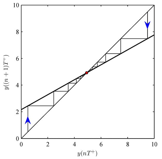
System (4) has a unique positive solution $y^{\ast }(t;\mu )$ if and only if

$${\displaystyle \prod _{h=1}^{m+1}}\left((1-p_N^{\left(h\right)}){\displaystyle \prod _{l=1}^{m_h}}(1+p_l^{\left(h\right)})\right)e^{\mu T}<1,$$

(10)

and for every solution $y(t;\mu )$ of (4), it follows that $\underset{t\to +\infty }{lim}(y(t;\mu )-y^{\ast }(t;\mu ))=0$ (see Figure 1).

Figure 1. Dynamic cobweb method to show the relationship of $y\left(n{T}^{+}\right)$ and $y\left((n+1)T^{+}\right)$ corresponding to the special case demonstrated in system (52). The baseline parameter values are fixed as follows: $D=0.08$, $p_N=0.45$, $p_M=0.05$, $q=2$, $T=1$, and $m=2$.

Proof. 

From (4), we have

$$\left\{\begin{array}{cccc}\hfill {\displaystyle \frac{dz\left(t\right)}{dt}}& =& \mu z\left(t\right),\hfill & t\notin nT+\left\{0,{\lambda }_1,{\lambda }_2,\cdots ,{\lambda }_m\right\},\hfill \\ \hfill & & & t\notin nT+\left\{{\tau }_1^{\left(j\right)},{\tau }_2^{\left(j\right)},\cdots ,{\tau }_{m_j}^{\left(j\right)}\right\},1\le j\le m+1,\hfill \\ \hfill z\left(t^{+}\right)& =& (1-p_N^{\left(i\right)})z\left(t\right),\hfill & t=nT+{\lambda }_i,1\le i\le m+1,\hfill \\ \hfill z\left(t^{+}\right)& =& (1+p_k^{\left(j\right)})z\left(t\right),\hfill & t\in nT+{\tau }_k^{\left(j\right)},1\le k\le m_j,1\le j\le m+1,\hfill \end{array}\right.$$

where $z\left(t\right)=y(t;\mu )-y^{\ast }(t;\mu )$. Similar to (9) and (8), it follows that

$$z\left(n{T}^{+}\right)={\displaystyle \prod _{h=1}^{m+1}}\left((1-p_N^{\left(h\right)}){\displaystyle \prod _{l=1}^{m_h}}(1+p_l^{\left(h\right)})\right)e^{\mu T}z\left((n-1)T^{+}\right).$$

(11)

Equations (5)–(8), (10), and (11) indicate that $\underset{t\to +\infty }{lim}z\left(t\right)=0$.

This completes the proof. □

In the following, we always assume that

$${\displaystyle \prod _{h=1}^{m+1}}\left((1-p_N^{\left(h\right)}){\displaystyle \prod _{l=1}^{m_h}}(1+p_l^{\left(h\right)})\right)e^{-DT}<1,$$

(12)

and denote

$$y^{\ast }\left(t\right)=y^{\ast }(t;-D).$$

3. Bifurcation of the Pest-Present Periodic Solution

Denote by $\Phi (t;t_0,X^0)$ the solution of the first two equations of (3) for the initial data $t=t_0$ and $X^0=(y^0,x^0)$; also,

$$\Phi (t;t_0,X^0)=(y(t;t_0,X^0),x(t;t_0,X^0)).$$

Additionally, we define some relevant mappings by

$$\left\{\begin{array}{ccc}\hfill P^{\left(i\right)}(y,x)& =& \left(\begin{array}{cc}1-p_N^{\left(i\right)}& 0\\ 0& 1-p_P^{\left(i\right)}\end{array}\right)\left(\begin{array}{c}y\\ x\end{array}\right),\hfill \\ \hfill & & i=1,\cdots ,m,m+1,\hfill \\ \hfill N_k^{\left(j\right)}(y,x)& =& \left(\begin{array}{cc}1+p_k^{\left(j\right)}& 0\\ 0& 1\end{array}\right)\left(\begin{array}{c}y\\ x\end{array}\right)+\left(\begin{array}{c}{q}_k^{\left(j\right)}\\ 0\end{array}\right),\hfill \\ \hfill & & 1\le k\le m_j,1\le j\le m+1,\hfill \end{array}\right.$$

(13)

and

$$\left\{\begin{array}{ccc}\hfill I_1^{\left(1\right)}\left(X^0\right)& =& N_1^{\left(1\right)}(\Phi ({\tau }_1^{\left(1\right)};X^0))\hfill \\ \hfill & \triangleq & {(I_{1_1}^{\left(1\right)}\left(X^0\right),I_{1_2}^{\left(1\right)}\left(X^0\right))}^T,\hfill \\ \hfill I_k^{\left(1\right)}\left(X^0\right)& =& N_k^{\left(1\right)}(\Phi ({\tau }_k^{\left(1\right)}-{\tau }_{k-1}^{\left(1\right)};I_{k-1}^{\left(1\right)}\left(X^0\right)))\hfill \\ \hfill & \triangleq & {(I_{k_1}^{\left(1\right)}\left(X^0\right),I_{k_2}^{\left(1\right)}\left(X^0\right))}^T,\hfill \\ \hfill & & 2\le k\le m_1,\hfill \\ \hfill {\Psi }^{\left(1\right)}\left(X^0\right)& =& P^{\left(1\right)}(\Phi ({\lambda }_1-{\tau }_{m_1}^{\left(1\right)};I_{m_1}^{\left(1\right)}\left(X^0\right)))\hfill \\ \hfill & \triangleq & ({\Psi }_1^{\left(1\right)}\left(X^0\right),{\Psi }_2^{\left(1\right)}\left(X^0\right)),\hfill \\ \hfill I_1^{\left(j\right)}\left(X^0\right)& =& N_1^{\left(j\right)}(\Phi ({\tau }_1^{\left(j\right)}-{\lambda }_{j-1};{\Psi }^{(j-1)}\left(X^0\right)))\hfill \\ \hfill & \triangleq & {(I_{1_1}^{\left(j\right)}\left(X^0\right),I_{1_2}^{\left(j\right)}\left(X^0\right))}^T,\hfill \\ \hfill I_k^{\left(j\right)}\left(X^0\right)& =& N_k^{\left(j\right)}(\Phi ({\tau }_k^{\left(j\right)}-{\tau }_{k-1}^{\left(j\right)};I_{k-1}^{\left(j\right)}\left(X^0\right)))\hfill \\ \hfill & \triangleq & {(I_{k_1}^{\left(j\right)}\left(X^0\right),I_{k_2}^{\left(j\right)}\left(X^0\right))}^T,\hfill \\ \hfill & & 2\le k\le m_j,\hfill \\ \hfill {\Psi }^{\left(j\right)}\left(X^0\right)& =& P^{\left(j\right)}(\Phi ({\lambda }_j-{\tau }_{m_j}^{\left(j\right)};I_{m_j}^{\left(j\right)}\left(X^0\right)))\hfill \\ \hfill & \triangleq & ({\Psi }_1^{\left(j\right)}\left(X^0\right),{\Psi }_2^{\left(j\right)}\left(X^0\right)),\hfill \\ \hfill & & 2\le j\le m+1.\hfill \end{array}\right.$$

(14)

Clearly, it follows that

$$\left\{\begin{array}{ccc}\hfill \left(\begin{array}{c}{I}_{1_1}^{\left(1\right)}\left(X^0\right)\\ I_{1_2}^{\left(1\right)}\left(X^0\right)\end{array}\right)& =& \left(\begin{array}{c}(1+p_1^{\left(1\right)})y({\tau }_1^{\left(1\right)};X^0)+q_1^{\left(1\right)}\\ x({\tau }_1^{\left(1\right)};X^0)\end{array}\right),\hfill \\ \hfill \left(\begin{array}{c}{I}_{k_1}^{\left(1\right)}\left(X^0\right)\\ I_{k_2}^{\left(1\right)}\left(X^0\right)\end{array}\right)& =& \left(\begin{array}{c}(1+p_k^{\left(1\right)})y({\tau }_k^{\left(1\right)}-{\tau }_{k-1}^{\left(1\right)};(I_{{(k-1)}_1}^{\left(1\right)}\left(X^0\right),I_{{(k-1)}_2}^{\left(1\right)}\left(X^0\right)))+q_k^{\left(1\right)}\\ x({\tau }_k^{\left(1\right)}-{\tau }_{k-1}^{\left(1\right)};(I_{{(k-1)}_1}^{\left(1\right)}\left(X^0\right),I_{{(k-1)}_2}^{\left(1\right)}\left(X^0\right)))\end{array}\right),\hfill \\ \hfill & & k=2,3,\cdots ,m_1,\hfill \\ \hfill \left(\begin{array}{c}{\Psi }_1^{\left(1\right)}\left(X^0\right)\\ {\Psi }_2^{\left(1\right)}\left(X^0\right)\end{array}\right)& =& \left(\begin{array}{c}(1-p_N^{\left(1\right)})y({\lambda }_1-{\tau }_{m_1}^{\left(1\right)};(I_{{\left(m_1\right)}_1}^{\left(1\right)}\left(X^0\right),I_{{\left(m_1\right)}_2}^{\left(1\right)}\left(X^0\right)))\\ (1-p_P^{\left(1\right)})x({\lambda }_1-{\tau }_{m_1}^{\left(1\right)};(I_{{\left(m_1\right)}_1}^{\left(1\right)}\left(X^0\right),I_{{\left(m_1\right)}_2}^{\left(1\right)}\left(X^0\right)))\end{array}\right),\hfill \\ \hfill \left(\begin{array}{c}{I}_{1_1}^{\left(j\right)}\left(X^0\right)\\ I_{1_2}^{\left(j\right)}\left(X^0\right)\end{array}\right)& =& \left(\begin{array}{c}(1+p_1^{\left(j\right)})y({\tau }_1^{\left(j\right)}-{\lambda }_{j-1};({\Psi }_1^{(j-1)}\left(X^0\right),{\Psi }_2^{(j-1)}\left(X^0\right)))+q_1^{\left(j\right)}\\ x({\tau }_1^{\left(j\right)}-{\lambda }_{j-1};({\Psi }_1^{(j-1)}\left(X^0\right),{\Psi }_2^{(j-1)}\left(X^0\right)))\end{array}\right),\hfill \\ \hfill \left(\begin{array}{c}{I}_{k_1}^{\left(j\right)}\left(X^0\right)\\ I_{k_2}^{\left(j\right)}\left(X^0\right)\end{array}\right)& =& \left(\begin{array}{c}(1+p_k^{\left(j\right)})y({\tau }_k^{\left(j\right)}-{\tau }_{k-1}^{\left(j\right)};(I_{{(k-1)}_1}^{\left(j\right)}\left(X^0\right),I_{{(k-1)}_2}^{\left(j\right)}\left(X^0\right)))+q_k^{\left(j\right)}\\ x({\tau }_k^{\left(j\right)}-{\tau }_{k-1}^{\left(j\right)};(I_{{(k-1)}_1}^{\left(j\right)}\left(X^0\right),I_{{(k-1)}_2}^{j)}\left(X^0\right)))\end{array}\right),\hfill \\ \hfill & & k=2,3,\cdots ,m_j,\hfill \\ \hfill \left(\begin{array}{c}{\Psi }_1^{\left(j\right)}\left(X^0\right)\\ {\Psi }_2^{\left(j\right)}\left(X^0\right)\end{array}\right)& =& \left(\begin{array}{c}(1-p_N^{\left(j\right)})y({\lambda }_j-{\tau }_{m_j}^{\left(j\right)};(I_{{\left(m_j\right)}_1}^{\left(j\right)}\left(X^0\right),I_{{\left(m_j\right)}_2}^{\left(j\right)}\left(X^0\right)))\\ (1-p_P^{\left(j\right)})x({\lambda }_j-{\tau }_{m_j}^{\left(j\right)};(I_{{\left(m_j\right)}_1}^{\left(j\right)}\left(X^0\right),I_{{\left(m_j\right)}_2}^{\left(j\right)}\left(X^0\right)))\end{array}\right),\hfill \\ \hfill & & j=2,3,\cdots ,m,m+1.\hfill \end{array}\right.$$

(15)

For $j=1,2,\cdots ,m,m+1$, it follows from (A7) that

$$\begin{array}{ccc}\hfill c^{\left(j\right)}\left(X_0^{\ast }\right)& =& (1-p_P^{\left(j\right)})e^{{\displaystyle {\int }_{{\lambda }_{j-1}^{+}}^{{\lambda }_j}(a-\frac{\alpha y^{\ast }\left(t\right)}{b})dt}},\hfill \end{array}$$

(16)

where $X_0^{\ast }={(y^{\ast }\left(0^{+}\right),0)}^T$. Then, from (A8), (12) and (16), we see that the two eigenvalues of the Jacobian matrix of the map $\Psi \left(X^0\right)$ at the point $X_0^{\ast }$ are

$$\left\{\begin{array}{ccc}\hfill {\mu }_1& =& {\displaystyle \prod _{h=1}^{m+1}}\left((1-p_N^{\left(h\right)}){\displaystyle \prod _{l=1}^{m_h}}(1+p_l^{\left(h\right)})\right)e^{-DT}<1,\hfill \\ \hfill {\mu }_2& =& \left({\displaystyle \prod _{j=1}^{m+1}}(1-p_P^{\left(j\right)})\right)e^{{\displaystyle {\int }_{0^{+}}^T(a-\frac{\alpha y^{\ast }\left(t\right)}{b})dt}},\hfill \end{array}\right.$$

(17)

which results in the following theorem [28]:

Theorem 1.

The pest-free periodic solution $(y^{\ast }\left(t\right),0)$ of system (3) is locally asymptotically stable provided that

$$R_s\triangleq \left({\displaystyle \prod _{j=1}^{m+1}}(1-p_P^{\left(j\right)})\right)e^{{\displaystyle {\int }_{0^{+}}^T(a-\frac{\alpha y^{\ast }\left(t\right)}{b})dt}}<1.$$

Using the comparison theorem, we find that [29,30].

Theorem 2.

The pest-free periodic solution $(y^{\ast }\left(t\right),0)$ of system (3) is globally attractive provided that

$$R_a\triangleq \left({\displaystyle \prod _{i=1}^{m+1}}(1-p_P^{\left(i\right)})\right)e^{{\displaystyle {\int }_{0^{+}}^T\left(a-\frac{\alpha y^{\ast }\left(t\right)}{b+K}\right)dt}}<1.$$

(18)

In fact, we can prove that a necessary condition for the bifurcation of a pest-present periodic solution is [31]

$$\begin{array}{c}\hfill {\mu }_2=\left({\displaystyle \prod _{j=1}^{m+1}}(1-p_P^{\left(j\right)})\right)e^{{\displaystyle {\int }_{0^{+}}^T(a-\frac{\alpha y^{\ast }\left(t\right)}{b})dt}}=1.\end{array}$$

(19)

According to Theorem 3, under a certain condition, (19) is sufficient as well.

To investigate the bifurcation of the pest-present periodic solution of system (3), we can consider the system as follows:

$$\left\{\begin{array}{c}\left.\begin{array}{ccc}\hfill {\displaystyle \frac{dy\left(t\right)}{dt}}& =& -Dy\left(t\right)+{\displaystyle \frac{\beta x\left(t\right)y\left(t\right)}{b+x\left(t\right)}},\hfill \\ \hfill {\displaystyle \frac{dx\left(t\right)}{dt}}& =& ax\left(t\right)(1-{\displaystyle \frac{x\left(t\right)}{K}})-{\displaystyle \frac{\alpha x\left(t\right)y\left(t\right)}{b+x\left(t\right)}},\hfill \end{array}\right\}\begin{array}{c}t\notin nT+\left\{0,L_{1}T,L_{2}T,\cdots ,L_{m}T\right\}\hfill \\ t\notin nT+\left\{l_1^{\left(j\right)}T,l_2^{\left(j\right)}T,\cdots ,l_{m_j}^{\left(j\right)}T\right\},1\le j\le m+1,\hfill \end{array}\hfill \\ \left.\begin{array}{ccc}\hfill y\left(t^{+}\right)& =& \left(1-p_N^{\left(i\right)}\right)y\left(t\right),\hfill \\ \hfill x\left(t^{+}\right)& =& \left(1-p_P^{\left(i\right)}\right)x\left(t\right),\hfill \end{array}\right\}t=nT+L_{i}T,1\le i\le m+1,\hfill \\ \left.\begin{array}{ccc}\hfill y\left(t^{+}\right)& =& \left(1+p_k^{\left(j\right)}\right)y\left(t\right)+q_k^{\left(j\right)},\hfill \\ \hfill x\left(t^{+}\right)& =& x\left(t\right),\hfill \end{array}\right\}t=nT+l_k^{\left(j\right)}T,1\le k\le m_j,1\le j\le m+1,\hfill \end{array}\right.$$

(20)

where

$$\left\{\begin{array}{c}0=L_0<L_1<L_2<\cdots <L_m<L_{m+1}=1,\hfill \\ L_{j-1}=l_0^{\left(j\right)}<l_1^{\left(j\right)}<l_2^{\left(j\right)}<\cdots <l_{m_j}^{\left(j\right)}<l_{m_j+1}^{\left(j\right)}=L_j,1\le j\le m+1.\hfill \end{array}\right.$$

Theorem 3.

Suppose that

$$\left\{\begin{array}{ccc}\hfill \left({\displaystyle \prod _{j=1}^{m+1}}(1-p_P^{\left(j\right)})\right)e^{{\displaystyle {\int }_{0^{+}}^T(a-\frac{\alpha y^{\ast }\left(t\right)}{b})dt}}& =& 1,\hfill \\ \hfill {\displaystyle \frac{ab}{K\alpha }}& \ge & {\displaystyle \frac{\underset{1\le j\le m+1}{max}\underset{1\le k\le m_j}{max}{y}^{\ast }\left(l_k^{\left(j\right)}{T}^{+}\right)}{b}},\hfill \end{array}\right.$$

(21)

holds, then the pest-free periodic solution $(y^{\ast }\left(t\right),0)$ of system (20) bifurcates into a pest-present periodic solution.

Proof. 

Assume that the period T involved in (21) is rewritten as $T_b$, i.e.,

$$\left\{\begin{array}{ccc}\hfill \left({\displaystyle \prod _{j=1}^{m+1}}(1-p_P^{\left(j\right)})\right)e^{{\displaystyle {\int }_{0^{+}}^{T_b}(a-\frac{\alpha y^{\ast }\left(t\right)}{b})dt}}& =& 1,\hfill \\ \hfill {\displaystyle \frac{ab}{K\alpha }}& \ge & {\displaystyle \frac{\underset{1\le j\le m+1}{max}\underset{1\le k\le m_j}{max}{y}^{\ast }\left(l_k^{\left(j\right)}{T}_b^{+}\right)}{b}}.\hfill \end{array}\right.$$

(22)

Denote

$$\begin{array}{ccc}\hfill G(T,X^0)& =& {\Psi }^{(m+1)}\left(X^0\right)-X^0\hfill \\ \hfill & \triangleq & {(g_1(T,X^0),g_2(T,X^0))}^T.\hfill \end{array}$$

(23)

Then, it follows from (A2), (A4), (17), and (22) that

$$\begin{array}{ccc}\hfill D_{X^0}G\left(X_0^{\ast }\right)& =& D_{X^0}{\Psi }^{(m+1)}\left(X_0^{\ast }\right)-E_2\hfill \\ \hfill & =& \left(\begin{array}{cc}{a}_0^{\ast }& b_0^{\ast }\\ 0& 0\end{array}\right),\hfill \end{array}$$

(24)

where

$$\left\{\begin{array}{ccc}\hfill a_0^{\ast }& =& {\displaystyle \prod _{h=1}^{m+1}}\left((1-p_N^{\left(h\right)}){\displaystyle \prod _{l=1}^{m_h}}(1+p_l^{\left(h\right)})\right)e^{-D{T}_b}-1<0,\hfill \\ \hfill b_0^{\ast }& >& 0.\hfill \end{array}\right.$$

On the linear space ${\mathbb{R}}^2$ defined in the field $\mathbb{R}$, we can define a linear transformation $\mathcal{A}$ as follows:

$$\mathcal{A}(y,x)=D_{X^0}G\left(X_0^{\ast }\right)\left(\begin{array}{c}y\\ x\end{array}\right),$$

(25)

where $X={(y,x)}^T\in {\mathbb{R}}^2$. Then, for ${({\alpha }_0,{\beta }_0)}^T\in {\mathcal{A}}^{-1}\left(0\right)$, it follows that $\mathcal{A}({\alpha }_0,{\beta }_0)=0$; i.e.,

$$\left(\begin{array}{cc}{a}_0^{\ast }& b_0^{\ast }\\ 0& 0\end{array}\right)\left(\begin{array}{c}{\alpha }_0\\ {\beta }_0\end{array}\right)=0,$$

which implies that

$$\left\{\begin{array}{ccc}\hfill dim\left(\mathcal{A}\left({\mathbb{R}}^2\right)\right)& =& \mathrm{rank}\left(D_{X^0}G\left(X_0^{\ast }\right)\right)=1,\hfill \\ \hfill dim\left({\mathcal{A}}^{-1}\left(0\right)\right)& =& 2-dim\left(\mathcal{A}\left({\mathbb{R}}^2\right)\right)=1,\hfill \end{array}\right.$$

and a basis in ${\mathcal{A}}^{-1}\left(0\right)$ is $V_p={({\displaystyle \frac{b_0^{\ast }}{-a_0^{\ast }}},1)}^T$.

On the other hand, it follows from (24) and (25) that $\mathcal{A}\left({\mathbb{R}}^2\right)=\left\{\left.{(y,0)}^T\right|y\in \mathbb{R}\right\}$, which possesses a basis $V_f^{\prime }={(a_0^{\ast },0)}^T$. Let $\mathcal{A}({\alpha }_1,{\beta }_1)=V_f^{\prime }$, i.e.,

$$\left(\begin{array}{cc}{a}_0^{\ast }& b_0^{\ast }\\ 0& 0\end{array}\right)\left(\begin{array}{c}{\alpha }_1\\ {\beta }_1\end{array}\right)=\left(\begin{array}{c}{a}_0^{\ast }\\ 0\end{array}\right).$$

Then, we can take ${({\alpha }_1,{\beta }_1)}^T={(1,0)}^T\triangleq V_f$. Then, a group of bases of the linear space ${\mathbb{R}}^2$ can be taken as

$$\left\{\begin{array}{ccc}\hfill V_p& =& {({\displaystyle \frac{b_0^{\ast }}{-a_0^{\ast }}},1)}^T,\hfill \\ \hfill V_f& =& {(1,0)}^T.\hfill \end{array}\right.$$

Let $X^0=c_p{V}_p+c_f{V}_f$, where $c_p,c_f\in \mathbb{R}$, and

$$\left\{\begin{array}{ccc}\hfill f_1(T,c_p,c_f)& =& g_1(T,c_p{V}_p+c_f{V}_f),\hfill \\ \hfill f_2(T,c_p,c_f)& =& g_2(T,c_p{V}_p+c_f{V}_f).\hfill \end{array}\right.$$

(26)

It follows from (23), (24), and (26) that

$$\left\{\begin{array}{ccc}\hfill f_1(T_b,0,y^{\ast }\left(0^{+}\right))& =& 0,\hfill \\ \hfill {\displaystyle \frac{\partial f_1}{\partial c_f}}(T_b,0,y^{\ast }\left(0^{+}\right))& =& {\displaystyle \frac{\partial g_1}{\partial y^0}}(T_b,(y^{\ast }\left(0^{+}\right),0))\hfill \\ \hfill & =& a_0^{\ast }<0.\hfill \end{array}\right.$$

According to the implicit function theorem, there exists a unique function $c_f=c_f(T,c_p)$ in some neighborhood of $(T_b,0,y^{\ast }\left(0^{+}\right))$ such that

$$\left\{\begin{array}{ccc}\hfill c_f(T_b,0)& =& y^{\ast }\left(0^{+}\right),\hfill \\ \hfill f_1(T,c_p,c_f(T,c_p))& =& 0.\hfill \end{array}\right.$$

(27)

Let us denote

$$f(T,c_p)=f_2(T,c_p,c_f(T,c_p)).$$

(28)

Thus, from (20), (23), (24) and (26)–(28), we see that

$$\left\{\begin{array}{ccc}\hfill f(T_b,0)& =& g_2(T_b,X_0^{\ast })\hfill \\ \hfill & =& 0,\hfill \\ \hfill {\displaystyle \frac{\partial f}{\partial c_p}}(T_b,0)& =& {\left.{\displaystyle \frac{\partial g_2}{\partial y^0}}(T,c_p{V}_p+c_f(T,c_p)V_f)\right|}_{(T,c_p)=(T_b,0)}\left({\displaystyle \frac{b_0^{\ast }}{-a_0^{\ast }}}+{\displaystyle \frac{\partial c_f(T_b,0)}{\partial c_p}}\right)\hfill \\ \hfill & & +{\left.{\displaystyle \frac{\partial g_2}{\partial x^0}}(T,c_p{V}_p+c_f{V}_f)\right|}_{(T,c_p)=(T_b,0)}\hfill \\ \hfill & =& 0,\hfill \\ \hfill {\displaystyle \frac{{\partial }^{n}f}{\partial T^n}}(T,0)& =& {\displaystyle \frac{{\partial }^n}{\partial T^n}}\left(g_2(T,c_f(T,0)V_f)\right)\hfill \\ \hfill & =& 0,n=1,2,\cdots .\hfill \end{array}\right.$$

(29)

From (29), we can determine the Taylor series of f at point $(T_b,0)$ as follows:

$$f(T,c_p)=c_p\widehat{f}(T,c_p),$$

where

$$\begin{array}{ccc}\hfill \widehat{f}(T,c_p)& =& {\displaystyle \frac{1}{2!}}\left(2(T-T_b){\displaystyle \frac{{\partial }^{2}f}{\partial T\partial c_p}}(T_b,0)+c_p{\displaystyle \frac{{\partial }^{2}f}{\partial c_p^2}}(T_b,0)\right)\hfill \\ \hfill & & +\cdots \hfill \\ \hfill & & +{\displaystyle \frac{1}{n!}}\left(C_n^1{(T-T_b)}^{n-1}{\displaystyle \frac{{\partial }^{n}f}{\partial T^{n-1}\partial c_p}}(T_b,0)\right.+C_n^2{(T-T_b)}^{n-2}{c}_p{\displaystyle \frac{{\partial }^{n}f}{\partial T^{n-2}\partial c_p^2}}(T_b,0)\hfill \\ \hfill & & \left.+\cdots +c_p^{n-1}{\displaystyle \frac{{\partial }^{n}f}{\partial c_p^n}}(T_b,0)\right)\hfill \\ \hfill & & +\cdots .\hfill \end{array}$$

From (14), (23), (26), and (28), we see that

$$f(T,c_p)={\Psi }_2^{(m+1)}(c_p{V}_p+c_f(T,c_p)V_f)-c_p,$$

(30)

and, thus, it follows from (30), (A27), and (A33) that

$$\left\{\begin{array}{ccc}\hfill {\displaystyle \frac{{\partial }^{2}f(T_b,0)}{\partial c_p^2}}& =& {\left.{\displaystyle \frac{{\partial }^2}{\partial c_p^2}}\left({\Psi }_2^{(m+1)}(c_p{V}_p+c_f(T,c_p)V_f)\right)\right|}_{(T,c_p)=(T_b,0)}\hfill \\ \hfill & <& 0,\hfill \\ \hfill {\displaystyle \frac{{\partial }^{2}f(T_b,0)}{\partial c_p\partial T}}& =& {\left.{\displaystyle \frac{{\partial }^2}{\partial c_p\partial T}}\left({\Psi }_2^{(m+1)}(c_p{V}_p+c_f(T,c_p)V_f)\right)\right|}_{(T,c_p)=(T_b,0)}\hfill \\ \hfill & >& 0.\hfill \end{array}\right.$$

(31)

Note that

$$\begin{array}{ccc}\hfill {\displaystyle \frac{\partial \widehat{f}}{\partial c_p}}(T,c_p)& =& {\displaystyle \frac{1}{2!}}{\displaystyle \frac{{\partial }^{2}f}{\partial c_p^2}}(T_b,0)\hfill \\ \hfill & & +\cdots \hfill \\ \hfill & & +{\displaystyle \frac{1}{n!}}\left(C_n^2{(T-T_b)}^{n-2}{\displaystyle \frac{{\partial }^{n}f}{\partial T^{n-2}\partial c_p^2}}(T_b,0)+\cdots +(n-1)c_p^{n-2}{\displaystyle \frac{{\partial }^{n}f}{\partial c_p^n}}(T_b,0)\right)\hfill \\ \hfill & & +\cdots ,\hfill \end{array}$$

and furthermore,

$${\displaystyle \frac{\partial \widehat{f}}{\partial c_p}}(T_b,0)={\displaystyle \frac{1}{2!}}{\displaystyle \frac{{\partial }^{2}f}{\partial c_p^2}}(T_b,0)<0$$

(32)

based on (31). In addition, $\widehat{f}(T_b,0)=0$. Then, there exists a unique function $c_p=c_p\left(T\right)$ in some neighborhood of $(T_b,0)$ such that

$$\left\{\begin{array}{ccc}\hfill c_p\left(T_b\right)& =& 0,\hfill \\ \hfill \widehat{f}(T,c_p\left(T\right))& =& 0.\hfill \end{array}\right.$$

(33)

It follows from (33) that

$${\displaystyle \frac{\partial \widehat{f}}{\partial T}}(T_b,0)+{\displaystyle \frac{\partial \widehat{f}}{\partial c_p}}(T_b,0){\displaystyle \frac{d{c}_p\left(T_b\right)}{dT}}=0.$$

(34)

Then, from (31)–(34), we have

$$\begin{array}{ccc}\hfill \underset{T\to T_b^{+}}{lim}{\displaystyle \frac{c_p\left(T\right)}{T-T_b}}& =& \underset{T\to T_b^{+}}{lim}{\displaystyle \frac{c_p\left(T\right)-c_p\left(T_b\right)}{T-T_b}}\hfill \\ \hfill & =& {\displaystyle \frac{\frac{\partial \widehat{f}}{\partial T}(T_b,0)}{-\frac{\partial \widehat{f}}{\partial c_p}(T_b,0)}}\hfill \\ \hfill & =& {\displaystyle \frac{\frac{{\partial }^{2}f}{\partial c_p\partial T}(T_b,0)}{-\frac{\partial \widehat{f}}{\partial c_p}(T_b,0)}}\hfill \\ \hfill & >& 0.\hfill \end{array}$$

Thus, there exists a $\Delta T>0$ such that when $T\in (T_b,T_b+\Delta T)$, it follows that $c_p\left(T\right)>0$. Then, a pest-present periodic solution emerges.

This completes the proof. □

4. Existence and Global Attractiveness of the Pest-Present Periodic Solution of System (3)

In this section, we provide some sufficient conditions ensuring the permanence and the existence and global attractiveness of the pest-present periodic solution of system (3).

Theorem 4.

Assume that

$$\left\{\begin{array}{ccc}{\displaystyle \prod _{h=1}^{m+1}}\left((1-p_N^{\left(h\right)}){\displaystyle \prod _{l=1}^{m_h}}(1+p_l^{\left(h\right)})\right)e^{(-D+{\displaystyle \frac{\beta K}{b+K}})T}\hfill & <& 1,\hfill \\ R_s=\left({\displaystyle \prod _{j=1}^{m+1}}(1-p_P^{\left(j\right)})\right)e^{{\displaystyle {\int }_{0^{+}}^T(a-\frac{\alpha y^{\ast }\left(t\right)}{b})dt}}\hfill & >& 1,\hfill \end{array}\right.$$

(35)

we draw the following conclusions:

(i)

The system (3) is permanent;

(ii)

If

$${\displaystyle \prod _{h=1}^{m+1}}\left({\displaystyle \prod _{l=1}^{m_h}}(1+p_l^{\left(h\right)})\right)e^{{\widehat{C}}_{1}T}<1$$

(36)

holds, where

$${\widehat{C}}_1\triangleq max\left\{-D+{\displaystyle \frac{\beta K}{b+K}}+{\displaystyle \frac{\alpha }{b+m_P}},m_P\left({\displaystyle \frac{(b\beta +\alpha )M_N}{{(b+m_P)}^2}}-{\displaystyle \frac{a}{K}}\right)\right\},$$

then there exists a globally attractive pest-present periodic solution for system (3).

Proof. 

$\left(i\right)$ According to Lemmas 2, (3), and (35), we may assume that $m_N\le y\left(t\right)\le M_N$ for $t\ge 0$, where

$$\left\{\begin{array}{ccc}\hfill m_N& =& \underset{1\le j\le m+1}{min}\underset{1\le k\le m_j}{min}{y}^{\ast }\left(l_k^{\left(j\right)}T\right)-{\epsilon }_1,\hfill \\ \hfill M_N& =& \underset{1\le j\le m+1}{max}\underset{t\in [{\lambda }_{j-1}^{+},{\tau }_1^{\left(j\right)}]\cup \cdots \cup [{\left({\tau }_{m_j}^{\left(j\right)}\right)}^{+},{\lambda }_j]}{max}{y}^{\ast }\left(t;-D+{\displaystyle \frac{\beta K}{b+K}}\right)+{\epsilon }_2,\hfill \end{array}\right.$$

with ${\epsilon }_2>0$ and ${\epsilon }_1\in \left(0,\underset{1\le j\le m+1}{min}\underset{1\le k\le m_j}{min}{y}^{\ast }\left(l_k^{\left(j\right)}T\right)\right)$. According to the definition of the permanence of system (3), we only need to find $m_P>0$ such that $x\left(t\right)\ge m_P$ for a sufficiently large t.

In view of (12) and (35), we can choose $m_0>0$ and ${\epsilon }_3>0$ such that

$$\left\{\begin{array}{ccc}\hfill {\displaystyle \prod _{h=1}^{m+1}}\left((1-p_N^{\left(h\right)}){\displaystyle \prod _{l=1}^{m_h}}(1+p_l^{\left(h\right)})\right)e^{(-D+{\displaystyle \frac{\beta m_0}{b+m_0}})T}& <& 1,\hfill \\ \hfill \zeta & >& 1,\hfill \end{array}\right.$$

where

$$\zeta \triangleq \left({\displaystyle \prod _{i=1}^{m+1}}(1-p_P^{\left(i\right)})\right)e^{{\displaystyle {\int }_{0^{+}}^T\left[a-\frac{a{m}_0}{K}-\frac{\alpha }{b}\left(y^{\ast }\left(t;-D+\frac{\beta m_0}{b+m_0}\right)+{\epsilon }_3\right)\right]dt}}.$$

Consider the following system:

$$\left\{\begin{array}{c}\begin{array}{ccc}\hfill {\displaystyle \frac{dy\left(t\right)}{dt}}& =& (-D+{\displaystyle \frac{\beta m_0}{b+m_0}})y\left(t\right),\hfill \\ \hfill & & \\ \hfill & & \\ \hfill y\left(t^{+}\right)& =& (1-p_N^{\left(i\right)})y\left(t\right),\hfill \\ \hfill y\left(t^{+}\right)& =& (1+p_k^{\left(j\right)})y\left(t\right)+q_k^{\left(j\right)},\hfill \end{array}\begin{array}{c}t\notin nT+\left\{0,{\lambda }_1,{\lambda }_1,\cdots ,{\lambda }_m\right\},\hfill \\ t\notin nT+\left\{{\tau }_1^{\left(j\right)},{\tau }_2^{\left(j\right)},\cdots ,{\tau }_{m_j}^{\left(j\right)}\right\},\hfill \\ 1\le j\le m+1,\hfill \\ t=nT+{\lambda }_i,1\le i\le m+1,\hfill \\ t=nT+{\tau }_k^{\left(j\right)},1\le k\le m_j,1\le j\le m+1.\hfill \end{array}\hfill \end{array}\right.$$

According to Lemma 2, we see that $\underset{t\to +\infty }{lim}(y(t;-D+{\displaystyle \frac{\beta m_0}{b+m_0}})-y^{\ast }(t;-D+{\displaystyle \frac{\beta m_0}{b+m_0}}))=0$. Then, there exists a $t_3>0$ such that

$$y(t;-D+{\displaystyle \frac{\beta m_0}{b+m_0}})<y^{\ast }(t;-D+{\displaystyle \frac{\beta m_0}{b+m_0}})+{\epsilon }_3,\mathrm{for}t>t_3.$$

(37)

Similar to (44), we can prove that there exists a $t_4>t_3$ such that $x\left(t_4\right)\ge m_0$. Without loss of generality, assume that there exists some $t>t_4$ such that $x\left(t\right)<m_0$. Set $t^{\ast }=inf\left\{\left.t\right|t>t_4,x\left(t\right)<m_0\right\}$; then, $t^{\ast }\ge t_4>t_3$. Then, $x\left(t\right)\ge m_0$ holds for $t\in (t_4,t^{\ast }]$, and assume that $t^{\ast }\in (n_{1}T,(n_1+1)T]$, where $n_1\in {\mathrm{Z}}_{+}$.

Consider the following system:

$$\left\{\begin{array}{c}\begin{array}{ccc}\hfill {\displaystyle \frac{dx\left(t\right)}{dt}}& =& x\left(t\right)\left(\underset{\triangleq \eta }{\underbrace{a-{\displaystyle \frac{a{m}_0}{K}}-max\left\{{\displaystyle \frac{\alpha M_N}{b}},a\right\}}}\right)\hfill \\ \hfill & \triangleq & x\left(t\right)\eta ,\hfill \\ \hfill & & \\ \hfill & & \\ \hfill x\left(t^{+}\right)& =& (1-p_P^{\left(i\right)}))x\left(t\right),\hfill \\ \hfill x\left(t^{+}\right)& =& x\left(t\right),\hfill \\ \hfill x\left(n_1{T}^{+}\right)& =& {\displaystyle \frac{m_0}{2}},\hfill \end{array}\begin{array}{c}\\ \\ t\notin nT+\left\{0,{\lambda }_1,{\lambda }_1,\cdots ,{\lambda }_m\right\},\hfill \\ t\notin nT+\left\{{\tau }_1^{\left(j\right)},{\tau }_2^{\left(j\right)},\cdots ,{\tau }_{m_j}^{\left(j\right)}\right\},\hfill \\ 1\le j\le m+1,\hfill \\ t=nT+{\lambda }_i,1\le i\le m+1,\hfill \\ t=nT+{\tau }_k^{\left(j\right)},1\le k\le m_j,1\le j\le m+1,\hfill \end{array}\hfill \end{array}\right.$$

(38)

where $\eta =a-{\displaystyle \frac{a{m}_0}{K}}-max\left\{{\displaystyle \frac{\alpha M_N}{b}},a\right\}<0$. Then, it follows that

$$\begin{array}{ccc}\hfill \widehat{x}\left(t^{\ast }\right)& <& \widehat{x}\left(n_1{T}^{+}\right)\hfill \\ \hfill & =& {\displaystyle \frac{m_0}{2}}\hfill \\ \hfill & <& x\left(t^{\ast }\right),\hfill \end{array}$$

(39)

where $\widehat{x}\left(t\right)$ is a solution of system (38).

We claim that $x\left(t\right)\ge \widehat{x}\left(t\right)$ holds within the interval $(t^{\ast },+\infty )$. By contrast, assume that there exists a $t_5>t^{\ast }$ such that $x\left(t_5\right)<\widehat{x}\left(t_5\right)$. Set

$$t^{\ast \ast }=inf\left\{\left.t\right|t>t^{\ast },x\left(t\right)<\widehat{x}\left(t\right)\right\}.$$

From (39), $x\left({t^{\ast }}^{+}\right)>\widehat{x}\left({t^{\ast }}^{+}\right)$. Then, $t^{\ast \ast }>t^{\ast }$, and it follows for the interval $(t^{\ast },t^{\ast \ast }]$ that $x\left(t\right)\ge \widehat{x}\left(t\right)$. Obviously, it is impossible that $x\left(t^{\ast \ast }\right)>\widehat{x}\left(t^{\ast \ast }\right)$. Therefore, assume that $x\left(t^{\ast \ast }\right)=\widehat{x}\left(t^{\ast \ast }\right)<\widehat{x}\left(n_1{T}^{+}\right)={\displaystyle \frac{m_0}{2}}$. Then, $x\left({t^{\ast \ast }}^{+}\right)=\widehat{x}\left({t^{\ast \ast }}^{+}\right)<m_0$, and furthermore, there exists a $\delta >0$ such that when $t\in (t^{\ast \ast },t^{\ast \ast }+\delta )$, it follows that $x\left(t\right)<m_0$. Moreover, it follows for the interval $(t^{\ast \ast },t^{\ast \ast }+\delta )$ that

$$\left\{\begin{array}{c}\begin{array}{ccc}\hfill {\displaystyle \frac{dx\left(t\right)}{dt}}& \ge & x\left(t\right)\left(\underset{\triangleq \eta }{\underbrace{a-{\displaystyle \frac{a{m}_0}{K}}-max\left\{{\displaystyle \frac{\alpha M_N}{b}},a\right\}}}\right)\hfill \\ \hfill & \triangleq & x\left(t\right)\eta ,\hfill \\ \hfill & & \\ \hfill & & \\ \hfill x\left(t^{+}\right)& =& (1-p_P^{\left(i\right)})x\left(t\right),\hfill \\ \hfill x\left(t^{+}\right)& =& x\left(t\right),\hfill \end{array}\begin{array}{c}\\ \\ \\ t\notin nT+\left\{0,{\lambda }_1,{\lambda }_1,\cdots ,{\lambda }_m\right\},\hfill \\ t\notin nT+\left\{{\tau }_1^{\left(j\right)},{\tau }_2^{\left(j\right)},\cdots ,{\tau }_{m_j}^{\left(j\right)}\right\},\hfill \\ 1\le j\le m+1,\hfill \\ t=nT+{\lambda }_i,1\le i\le m+1,\hfill \\ t=nT+{\tau }_k^{\left(j\right)},1\le k\le m_j,1\le j\le m+1.\hfill \end{array}\hfill \end{array}\right.$$

(40)

Thus, $x\left(t\right)\ge \widehat{x}\left(t\right)$ is valid in the interval $(t^{\ast \ast },t^{\ast \ast }+\delta )$, contradicting the definition of $t^{\ast \ast }=inf\left\{\left.t\right|t>t^{\ast },x\left(t\right)<\widehat{x}\left(t\right)\right\}$.

Consider the following system:

$$\left\{\begin{array}{c}\begin{array}{ccc}\hfill {\displaystyle \frac{dx\left(t\right)}{dt}}& =& x\left(t\right)\left[a-{\displaystyle \frac{a{m}_0}{K}}-{\displaystyle \frac{\alpha }{b}}\left(y^{\ast }\left(t;-D+{\displaystyle \frac{\beta m_0}{b+m_0}}\right)+{\epsilon }_3\right)\right],\hfill \\ \hfill & & \\ \hfill & & \\ \hfill x\left(t^{+}\right)& =& (1-p_P^{\left(i\right)}))x\left(t\right),\hfill \\ \hfill x\left(t^{+}\right)& =& x\left(t\right),\hfill \\ \hfill x\left((n_1+1)T\right)& =& \widehat{x}\left((n_1+1)T\right).\hfill \end{array}\begin{array}{c}t\notin nT+\left\{0,{\lambda }_1,{\lambda }_1,\cdots ,{\lambda }_m\right\},\hfill \\ t\notin nT+\left\{{\tau }_1^{\left(j\right)},{\tau }_2^{\left(j\right)},\cdots ,{\tau }_{m_j}^{\left(j\right)}\right\},\hfill \\ 1\le j\le m+1,\hfill \\ t=nT+{\lambda }_i,1\le i\le m+1,\hfill \\ t=nT+{\tau }_k^{\left(j\right)},1\le k\le m_j,1\le j\le m+1,\hfill \end{array}\hfill \end{array}\right.$$

(41)

We have

$$\tilde{x}\left((n+1)T\right)=\tilde{x}\left(nT\right)\zeta ,$$

where $\tilde{x}\left(t\right)$ is a solution of system (41). Thus, it follows that

$$\begin{array}{ccc}\hfill \tilde{x}((n_1+1)T+n_{2}T)& =& \tilde{x}\left((n_1+1)T\right){\zeta }^{n_2}\hfill \\ \hfill & =& \widehat{x}\left((n_1+1)T\right){\zeta }^{n_2}\hfill \\ \hfill & >& m_0,\hfill \end{array}$$

(42)

where

$$n_2=\left[{\displaystyle \frac{ln\frac{m_0}{\widehat{x}\left((n_1+1)T\right)}}{ln\zeta }}\right]+1.$$

Without loss of generality, assume that for all $t\in (t^{\ast },(n_1+1)T]$, $x\left(t\right)<m_0$. We claim that there exists a $t_6\in ((n_1+1)T,(n_1+1)T+n_{2}T)$ such that $x\left(t_6\right)>m_0$. By contrast, assume that $x\left(t\right)\le m_0$ for all $t\in ((n_1+1)T,(n_1+1)T+n_{2}T]$. Then, when $t\in ((n_1+1)T,(n_1+1)T+n_{2}T]$, it follows from (3) and (37) that

$$\left\{\begin{array}{c}\begin{array}{ccc}\hfill {\displaystyle \frac{dx\left(t\right)}{dt}}& \ge & x\left(t\right)\left[a-{\displaystyle \frac{a{m}_0}{K}}-{\displaystyle \frac{\alpha }{b}}\left(y^{\ast }\left(t;-D+{\displaystyle \frac{\beta m_0}{b+m_0}}\right)+{\epsilon }_3\right)\right],\hfill \\ \hfill & & \\ \hfill & & \\ \hfill x\left(t^{+}\right)& =& (1-p_P^{\left(i\right)}))x\left(t\right),\hfill \\ \hfill x\left(t^{+}\right)& =& x\left(t\right),\hfill \end{array}\begin{array}{c}t\notin nT+\left\{0,{\lambda }_1,{\lambda }_1,\cdots ,{\lambda }_m\right\},\hfill \\ t\notin nT+\left\{{\tau }_1^{\left(j\right)},{\tau }_2^{\left(j\right)},\cdots ,{\tau }_{m_j}^{\left(j\right)}\right\},\hfill \\ 1\le j\le m+1,\hfill \\ t=nT+{\lambda }_i,1\le i\le m+1,\hfill \\ t=nT+{\tau }_k^{\left(j\right)},1\le k\le m_j,1\le j\le m+1.\hfill \end{array}\hfill \end{array}\right.$$

(43)

Note that $x((n_1+1)T^{+};t^{\ast },x\left(t^{\ast }\right))\ge \widehat{x}\left((n_1+1)T^{+}\right)$. It follows from (41)–(43) that

$$\begin{array}{ccc}\hfill x((n_1+1)T+n_{2}T)& \ge & \tilde{x}((n_1+1)T+n_{2}T)\hfill \\ \hfill & >& m_0,\hfill \end{array}$$

(44)

which is a contradiction.

For the interval $(t^{\ast },t_6)$,

$$\begin{array}{ccc}\hfill x\left(t\right)& \ge & \widehat{x}\left(t\right)\hfill \\ \hfill & >& \widehat{x}\left(t_6\right)\hfill \\ \hfill & >& \widehat{x}((n_1+1)T+n_{2}T)\triangleq m_P.\hfill \end{array}$$

For $t>t_6$, the same arguments can be continued because $x\left(t_6\right)>m_0$. $\left(ii\right)$ To investigate the existence and global attractiveness of the pest-present periodic solution of system (3), we only need to carry it out in the set S, where

$$S\triangleq \left\{\left.{(y\left(t\right),x\left(t\right))}^T\in {\mathbb{R}}_{+}^2\right|m_N\le y\left(t\right)\le M_N,m_P\le x\left(t\right)\le K\right\}.$$

(3) shows that when $t\notin nT+\left\{0,{\lambda }_1,{\lambda }_2,\cdots ,{\lambda }_m\right\}$ and $t\notin nT+\left\{{\tau }_1^{\left(j\right)},{\tau }_2^{\left(j\right)},\cdots ,{\tau }_{m_j}^{\left(j\right)}\right\}$, where $1\le j\le m+1$, we have the following:

$$\left\{\begin{array}{ccc}\hfill {\displaystyle \frac{dy\left(t\right)}{dt}}& =& -Dy\left(t\right)+{\displaystyle \frac{\beta x\left(t\right)y\left(t\right)}{b+x\left(t\right)}},\hfill \\ \hfill {\displaystyle \frac{dlnx\left(t\right)}{dt}}& =& a(1-{\displaystyle \frac{x\left(t\right)}{K}})-{\displaystyle \frac{\alpha y\left(t\right)}{b+x\left(t\right)}}.\hfill \end{array}\right.$$

(45)

Let us assume that $(y_i\left(t\right),x_i\left(t\right))\in S$, $i=1,2$ are two solutions of system (3). Then, when

$$\left\{\begin{array}{cc}t\notin nT+\left\{0,{\lambda }_1,{\lambda }_2,\cdots ,{\lambda }_m\right\},\hfill & \\ t\notin nT+\left\{{\tau }_1^{\left(j\right)},{\tau }_2^{\left(j\right)},\cdots ,{\tau }_{m_j}^{\left(j\right)}\right\},\hfill & 1\le j\le m+1,\hfill \\ (y_2\left(t\right)-y_1\left(t\right))(x_2\left(t\right),x_1\left(t\right))\ne 0,\hfill \end{array}\right.$$

it follows from (45) that

$$\begin{array}{ccc}\hfill {\displaystyle \frac{d\left|y_2\left(t\right)-y_1\left(t\right)\right|}{dt}}& =& \mathrm{sgn}(y_2\left(t\right)-y_1\left(t\right))\left({\displaystyle \frac{d{y}_2\left(t\right)}{dt}}-{\displaystyle \frac{d{y}_1\left(t\right)}{dt}}\right)\hfill \\ \hfill & =& -D\left|y_2\left(t\right)-y_1\left(t\right)\right|+\mathrm{sgn}(y_2\left(t\right)-y_1\left(t\right))\left[{\displaystyle \frac{\beta x_2\left(t\right)y_2\left(t\right)}{b+x_2\left(t\right)}}-{\displaystyle \frac{\beta x_1\left(t\right)y_1\left(t\right)}{b+x_1\left(t\right)}}\right]\hfill \\ \hfill & =& -D\left|y_2\left(t\right)-y_1\left(t\right)\right|\hfill \\ \hfill & & +\mathrm{sgn}(y_2\left(t\right)-y_1\left(t\right))\left[{\displaystyle \frac{\beta {\eta }_1}{b+{\eta }_1}}(y_2\left(t\right)-y_1\left(t\right))+{\displaystyle \frac{b\beta {\xi }_1}{{(b+{\eta }_1)}^2}}(x_2\left(t\right)-x_1\left(t\right))\right]\hfill \\ \hfill & \le & (-D+{\displaystyle \frac{\beta {\eta }_1}{b+{\eta }_1}})\left|y_2\left(t\right)-y_1\left(t\right)\right|+{\displaystyle \frac{b\beta {\xi }_1}{{(b+{\eta }_1)}^2}}\left|x_2\left(t\right)-x_1\left(t\right)\right|,\hfill \end{array}$$

(46)

where $({\xi }_1,{\eta }_1)=(y_1\left(t\right),x_1\left(t\right))+{\theta }_1((y_2\left(t\right),x_2\left(t\right))-(y_1\left(t\right),x_1\left(t\right)))$, ${\theta }_1\in (0,1)$, and

$$\begin{array}{ccc}\hfill {\displaystyle \frac{d\left|ln{x}_2\left(t\right)-ln{x}_1\left(t\right)\right|}{dt}}& =& \mathrm{sgn}(x_2\left(t\right)-x_1\left(t\right))\left({\displaystyle \frac{dln{x}_2\left(t\right)}{dt}}-{\displaystyle \frac{dln{x}_1\left(t\right)}{dt}}\right)\hfill \\ \hfill & =& -{\displaystyle \frac{a}{K}}\left|x_2\left(t\right)-x_1\left(t\right)\right|\hfill \\ \hfill & & -\mathrm{sgn}(x_2\left(t\right)-x_1\left(t\right))\left[{\displaystyle \frac{\alpha y_2\left(t\right)}{b+x_2\left(t\right)}}-{\displaystyle \frac{\alpha y_1\left(t\right)}{b+x_1\left(t\right)}}\right]\hfill \\ \hfill & =& -{\displaystyle \frac{a}{K}}\left|x_2\left(t\right)-x_1\left(t\right)\right|\hfill \\ \hfill & & -\mathrm{sgn}(x_2\left(t\right)-x_1\left(t\right)){\displaystyle \frac{\alpha }{(b+x_2\left(t\right))(b+x_1\left(t\right))}}\hfill \\ \hfill & & \times \left[(b+x_1\left(t\right))(y_2\left(t\right)-y_1\left(t\right))-y_1\left(t\right)(x_2\left(t\right)-x_1\left(t\right))\right]\hfill \\ \hfill & \le & {\displaystyle \frac{\alpha }{b+x_2\left(t\right)}}\left|y_2\left(t\right)-y_1\left(t\right)\right|\hfill \\ \hfill & & +\left({\displaystyle \frac{\alpha y_1\left(t\right)}{(b+x_2\left(t\right))(b+x_1\left(t\right))}}-{\displaystyle \frac{a}{K}}\right)\left|x_2\left(t\right)-x_1\left(t\right)\right|.\hfill \end{array}$$

(47)

Note that

$$\left|ln{x}_2\left(t\right)-ln{x}_1\left(t\right)\right|\le {\displaystyle \frac{1}{m_P}}\left|x_2\left(t\right)-x_1\left(t\right)\right|.$$

(48)

Define

$$V\left(t\right)\triangleq \left|y_2\left(t\right)-y_1\left(t\right)\right|+\left|ln{x}_2\left(t\right)-ln{x}_1\left(t\right)\right|.$$

Then, it follows from (36) and (46)–(48) that

$$\begin{array}{ccc}\hfill {\displaystyle \frac{dV\left(t\right)}{dt}}& \le & (-D+{\displaystyle \frac{\beta {\eta }_1}{b+{\eta }_1}}+{\displaystyle \frac{\alpha }{b+x_2\left(t\right)}})\left|y_2\left(t\right)-y_1\left(t\right)\right|\hfill \\ \hfill & & +\left({\displaystyle \frac{b\beta {\xi }_1}{{(b+{\eta }_1)}^2}}+{\displaystyle \frac{\alpha y_1\left(t\right)}{(b+x_2\left(t\right))(b+x_1\left(t\right))}}-{\displaystyle \frac{a}{K}}\right)\left|x_2\left(t\right)-x_1\left(t\right)\right|\hfill \\ \hfill & \le & (-D+{\displaystyle \frac{\beta K}{b+K}}+{\displaystyle \frac{\alpha }{b+m_P}})\left|y_2\left(t\right)-y_1\left(t\right)\right|\hfill \\ \hfill & & +m_P\left({\displaystyle \frac{b\beta M_N}{{(b+m_P)}^2}}+{\displaystyle \frac{\alpha M_N}{{(b+m_P)}^2}}-{\displaystyle \frac{a}{K}}\right){\displaystyle \frac{1}{m_P}}\left|x_2\left(t\right)-x_1\left(t\right)\right|\hfill \\ \hfill & \le & (-D+{\displaystyle \frac{\beta K}{b+K}}+{\displaystyle \frac{\alpha }{b+m_P}})\left|y_2\left(t\right)-y_1\left(t\right)\right|\hfill \\ \hfill & & +m_P\left({\displaystyle \frac{(b\beta +\alpha )M_N}{{(b+m_P)}^2}}-{\displaystyle \frac{a}{K}}\right)\left|ln{x}_2\left(t\right)-ln{x}_1\left(t\right)\right|\hfill \\ \hfill & \le & {\widehat{C}}_{1}V\left(t\right).\hfill \end{array}$$

However, it is easy to verify that

$$\left\{\begin{array}{ccc}\hfill V\left(t^{+}\right)& =& \left|y_2\left(t^{+}\right)-y_1\left(t^{+}\right)\right|+\left|ln{x}_2\left(t^{+}\right)-ln{x}_1\left(t^{+}\right)\right|\hfill \\ \hfill & =& (1-p_N^{\left(i\right)})\left|y_2\left(t\right)-y_1\left(t\right)\right|+\left|ln{x}_2\left(t\right)-ln{x}_1\left(t\right)\right|\hfill \\ \hfill & \le & V\left(t\right),\hfill & t=nT+{\lambda }_i,1\le i\le m+1,\hfill \\ \hfill V\left(t^{+}\right)& =& \left|y_2\left(t^{+}\right)-y_1\left(t^{+}\right)\right|+\left|ln{x}_2\left(t^{+}\right)-ln{x}_1\left(t^{+}\right)\right|\hfill \\ \hfill & =& (1+p_k^{\left(j\right)})\left|y_2\left(t\right)-y_1\left(t\right)\right|+\left|ln{x}_2\left(t\right)-ln{x}_1\left(t\right)\right|\hfill \\ \hfill & \le & (1+p_k^{\left(j\right)})V\left(t\right),\hfill & t=nT+{\tau }_k^{\left(j\right)},1\le k\le m_j,1\le j\le m+1.\hfill \end{array}\right.$$

Similar to (11), we obtain

$$\begin{array}{ccc}\hfill V\left((n+1)T^{+}\right)& \le & {\displaystyle \prod _{h=1}^{m+1}}\left({\displaystyle \prod _{l=1}^{m_h}}(1+p_l^{\left(h\right)})\right)e^{{\widehat{C}}_{1}T}V\left(n{T}^{+}\right).\hfill \end{array}$$

(49)

For any solution ${(y\left(t\right),x\left(t\right))}^T\in S$ of system (3), it follows from (49) and (36) that

$$\begin{array}{ccc}\hfill {\rho }_n& \triangleq & \left|y\left((n+1)T^{+}\right)-y\left(n{T}^{+}\right)\right|+\left|lnx\left((n+1)T^{+}\right)-lnx\left(n{T}^{+}\right)\right|\hfill \\ \hfill & =& \left|y(n{T}^{+};(y\left(T^{+}\right),x\left(T^{+}\right)))-y\left(n{T}^{+}\right)\right|\hfill \\ \hfill & & +\left|lnx(n{T}^{+};(y\left(T^{+}\right),x\left(T^{+}\right)))-lnx\left(n{T}^{+}\right)\right|\hfill \\ \hfill & \le & {\displaystyle \prod _{h=1}^{m+1}}\left({\displaystyle \prod _{l=1}^{m_h}}(1+p_l^{\left(h\right)})\right)e^{{\widehat{C}}_{1}T}\hfill \\ \hfill & & \times \left(\left|y((n-1)T^{+};(y\left(T^{+}\right),x\left(T^{+}\right)))-y\left((n-1)T^{+}\right)\right|\right.\hfill \\ \hfill & & \left.+\left|lnx((n-1)T^{+};(y\left(T^{+}\right),x\left(T^{+}\right)))-lnx\left((n-1)T^{+}\right)\right|\right)\hfill \\ \hfill & =& {\displaystyle \prod _{h=1}^{m+1}}\left({\displaystyle \prod _{l=1}^{m_h}}(1+p_l^{\left(h\right)})\right)e^{{\widehat{C}}_{1}T}\hfill \\ \hfill & & \times \left(\left|y\left(n{T}^{+}\right)-y\left((n-1)T^{+}\right)\right|+\left|lnx\left(n{T}^{+}\right)-lnx\left((n-1)T^{+}\right)\right|\right)\hfill \\ \hfill & =& {\displaystyle \prod _{h=1}^{m+1}}\left({\displaystyle \prod _{l=1}^{m_h}}(1+p_l^{\left(h\right)})\right)e^{{\widehat{C}}_{1}T}{\rho }_{n-1}\hfill \\ \hfill & \triangleq & {\widehat{C}}_2{\rho }_{n-1},\hfill \end{array}$$

and furthermore,

$${\rho }_n\le {\widehat{C}}_2{\rho }_{n-1}\le \cdots \le {\widehat{C}}_2^n{\rho }_0,$$

(50)

where

$$\left\{\begin{array}{ccc}\hfill {\rho }_n& =& \left|y\left((n+1)T^{+}\right)-y\left(n{T}^{+}\right)\right|+\left|lnx\left((n+1)T^{+}\right)-lnx\left(n{T}^{+}\right)\right|,\hfill \\ \hfill {\widehat{C}}_2& =& {\displaystyle \prod _{h=1}^{m+1}}\left({\displaystyle \prod _{l=1}^{m_h}}(1+p_l^{\left(h\right)})\right)e^{{\widehat{C}}_{1}T}.\hfill \end{array}\right.$$

Then, for arbitrary $p>0$, it follows from (50) that

$$\begin{array}{cc}\hfill & \left|y\left((n+p)T^{+}\right)-y\left(n{T}^{+}\right)\right|+\left|lnx\left((n+p)T^{+}\right)-lnx\left(n{T}^{+}\right)\right|\hfill \\ \hfill \le & \left|y\left((n+p)T^{+}\right)-y\left((n+p-1)T^{+}\right)\right|\hfill \\ \hfill & +\left|lnx\left((n+p)T^{+}\right)-lnx\left((n+p-1)T^{+}\right)\right|\hfill \\ \hfill & +\left|y\left((n+p-1)T^{+}\right)-y\left((n+p-2)T^{+}\right)\right|\hfill \\ \hfill & +\left|lnx\left((n+p-1)T^{+}\right)-lnx\left((n+p-2)T^{+}\right)\right|\hfill \\ \hfill & +\cdots \hfill \\ \hfill & +\left|y\left((n+1)T^{+}\right)-y\left(n{T}^{+}\right)\right|+\left|lnx\left((n+1)T^{+}\right)-lnx\left(n{T}^{+}\right)\right|\hfill \\ \hfill =& {\rho }_{n+p-1}+{\rho }_{n+p-2}+\cdots +{\rho }_n\hfill \\ \hfill \le & ({\widehat{C}}_2^{n+p-1}+{\widehat{C}}_2^{n+p-2}+\cdots +{\widehat{C}}_2^n){\rho }_0\hfill \\ \hfill =& {\displaystyle \frac{{\widehat{C}}_2^n(1-{\widehat{C}}_2^p)}{1-{\widehat{C}}_2}}{\rho }_0\hfill \\ \hfill <& {\displaystyle \frac{{\widehat{C}}_2^n}{1-{\widehat{C}}_2}}{\rho }_0,\hfill \end{array}$$

which implies that $\left\{y\left(n{T}^{+}\right)\right\}$ and $\left\{lnx\left(n{T}^{+}\right)\right\}$ are both Cauchy sequences. Thus, both $\underset{n\to \infty }{lim}y\left(n{T}^{+}\right)$ and $\underset{n\to \infty }{lim}lnx\left(n{T}^{+}\right)$ exist.

Denote

$$\left\{\begin{array}{ccc}\hfill \underset{n\to \infty }{lim}y\left(n{T}^{+}\right)& =& y^{\prime },\hfill \\ \hfill \underset{n\to \infty }{lim}lnx\left(n{T}^{+}\right)& =& ln{x}^{\prime },\hfill \end{array}\right.$$

where $y^{\prime }\in [m_N,M_N]$, and

$$x^{\prime }=\underset{n\to \infty }{lim}x\left(n{T}^{+}\right)\in [m_P,K].$$

Then, it follows that

$$\left\{\begin{array}{ccc}\hfill & & \underset{n\to \infty }{lim}y\left(n{T}^{+}\right)\hfill \\ \hfill & =& \underset{n\to \infty }{lim}y(T^{+};(y\left((n-1)T^{+}\right),x\left((n-1)T^{+}\right)))\hfill \\ \hfill & =& y(T^{+};(\underset{n\to \infty }{lim}y\left((n-1)T^{+}\right),\underset{n\to \infty }{lim}x\left((n-1)T^{+}\right)))\hfill \\ \hfill & =& y(T^{+};(y^{\prime },x^{\prime })),\hfill \\ \hfill & & \underset{n\to \infty }{lim}lnx\left(n{T}^{+}\right)\hfill \\ \hfill & =& ln\underset{n\to \infty }{lim}x(T^{+};(y\left((n-1)T^{+}\right),x\left((n-1)T^{+}\right)))\hfill \\ \hfill & =& lnx(T^{+};(\underset{n\to \infty }{lim}y\left((n-1)T^{+}\right),\underset{n\to \infty }{lim}x\left((n-1)T^{+}\right)))\hfill \\ \hfill & =& lnx(T^{+};(y^{\prime },x^{\prime })).\hfill \end{array}\right.$$

Thus, we have

$$\left\{\begin{array}{ccc}\hfill y(T^{+};(y^{\prime },x^{\prime }))& =& y^{\prime },\hfill \\ \hfill x(T^{+};(y^{\prime },x^{\prime }))& =& x^{\prime }.\hfill \end{array}\right.$$

That is, ${(y^{\prime },x^{\prime })}^T\in S$ is a fixed point of the Poincaré map of system (3).

If ${(y^{″},x^{″})}^T\in S$ is a fixed point of the Poincaré map of system (3), then

$$\left\{\begin{array}{ccc}\hfill y(T^{+};(y^{″},x^{″}))& =& y^{″},\hfill \\ \hfill x(T^{+};(y^{″},x^{″}))& =& x^{″}.\hfill \end{array}\right.$$

Since

$$\begin{array}{ccc}\hfill & & \left|y^{″}-y^{\prime }\right|+\left|ln{x}^{″}-ln{x}^{\prime }\right|\hfill \\ \hfill & =& \left|y(T^{+};(y^{″},x^{″}))-y(T^{+};(y^{\prime },x^{\prime }))\right|\hfill \\ \hfill & & +\left|lnx(T^{+};(y^{″},x^{″}))-lnx(T^{+};(y^{\prime },x^{\prime }))\right|\hfill \\ \hfill & \le & {\widehat{C}}_2\left(\left|y(0^{+};(y^{″},x^{″}))-y(0^{+};(y^{\prime },x^{\prime }))\right|\right.\hfill \\ \hfill & & \left.+\left|lnx(0^{+};(y^{″},x^{″}))-lnx(0^{+};(y^{\prime },x^{\prime }))\right|\right)\hfill \\ \hfill & =& {\widehat{C}}_2(\left|y^{″}-y^{\prime }\right|+\left|ln{x}^{″}-ln{x}^{\prime }\right|),\hfill \end{array}$$

we have $y^{″}=y^{\prime }$ and $x^{″}=x^{\prime }$ because ${\widehat{C}}_2\in (0,1)$. Therefore, ${(y^{\prime },x^{\prime })}^T\in S$ is a unique fixed point of the Poincaré map of system (3).

Therefore, ${(y^{\prime },x^{\prime })}^T\in S$ is a globally attractive fixed point of the Poincaré map of system (3).

This completes the proof. □

Remark 1.

In fact, system (38) can be replaced by the following system:

$$\left\{\begin{array}{c}\begin{array}{ccc}\hfill {\displaystyle \frac{dx\left(t\right)}{dt}}& =& x\left(t\right)\left(\underset{\triangleq a_{-}}{\underbrace{min\left\{\underset{(y,x)\in [m_N,M_N]\times [0,K]}{min}\left\{a-{\displaystyle \frac{ax}{K}}-{\displaystyle \frac{\alpha y}{b+x}}\right\},0\right\}-ϵ}}\right)\hfill \\ \hfill & \triangleq & x\left(t\right)a_{-},\hfill \\ \hfill & & \\ \hfill & & \\ \hfill x\left(t^{+}\right)& =& (1-p_P^{\left(i\right)}))x\left(t\right),\hfill \\ \hfill x\left(t^{+}\right)& =& x\left(t\right),\hfill \\ \hfill x\left(n_1{T}^{+}\right)& =& {\displaystyle \frac{m_0}{2}},\hfill \end{array}\begin{array}{c}\\ \\ t\notin nT+\left\{0,{\lambda }_1,{\lambda }_1,\cdots ,{\lambda }_m\right\},\hfill \\ t\notin nT+\left\{{\tau }_1^{\left(j\right)},{\tau }_2^{\left(j\right)},\cdots ,{\tau }_{m_j}^{\left(j\right)}\right\},\hfill \\ 1\le j\le m+1,\hfill \\ t=nT+{\lambda }_i,1\le i\le m+1,\hfill \\ t=nT+{\tau }_k^{\left(j\right)},1\le k\le m_j,1\le j\le m+1,\hfill \end{array}\hfill \end{array}\right.$$

(51)

where $ϵ>0$ and $a_{-}=min\left\{\underset{(y,x)\in [m_N,M_N]\times [0,K]}{min}\left\{a-{\displaystyle \frac{ax}{K}}-{\displaystyle \frac{\alpha y}{b+x}}\right\},0\right\}-ϵ<0$. Similarly, we can also prove that $x\left(t\right)>\widehat{x}\left(t\right)$ holds in the interval $(t^{\ast },+\infty )$, where $\widehat{x}\left(t\right)$ is a solution of system (51).

We note that the first inequality of (35) can be inferred from (36), and

$$\left\{\begin{array}{ccc}\hfill \underset{m_0\to 0^{+}}{lim}\left(-D+{\displaystyle \frac{\beta K}{b+K}}+{\displaystyle \frac{\alpha }{b+m_P}}\right)& =& -D+{\displaystyle \frac{\beta K}{b+K}}+{\displaystyle \frac{\alpha }{b}},\hfill \\ \hfill \underset{(m_0,{\epsilon }_2)\to (0^{+},0^{+})}{lim}\left({\displaystyle \frac{(b\beta +\alpha )M_N}{{(b+m_P)}^2}}-{\displaystyle \frac{a}{K}}\right)& =& {\displaystyle \frac{b\beta +\alpha }{b^2}}\underset{1\le j\le m+1}{max}\underset{t\in [{\lambda }_{j-1}^{+},{\tau }_1^{\left(j\right)}]\cup \cdots \cup [{\left({\tau }_{m_j}^{\left(j\right)}\right)}^{+},{\lambda }_j]}{max}{y}^{\ast }(t;-D+{\displaystyle \frac{\beta K}{b+K}})-{\displaystyle \frac{a}{K}}.\hfill \end{array}\right.$$

Then, the following claim is valid:

Corollary 1.

Let us assume that $p_M=0$, and that the second inequality of (35) and

$$\left\{\begin{array}{ccc}\hfill -D+{\displaystyle \frac{\beta K}{b+K}}+{\displaystyle \frac{\alpha }{b}}& <& 0,\hfill \\ \hfill {\displaystyle \frac{b\beta +\alpha }{b^2}}\underset{1\le j\le m+1}{max}\underset{1\le k\le m_j}{max}{y}^{\ast }\left({\left({\tau }_k^{\left(j\right)}\right)}^{+};-D+{\displaystyle \frac{\beta K}{b+K}}\right)-{\displaystyle \frac{a}{K}}& <& 0,\hfill \end{array}\right.$$

hold; then, there exists a globally attractive pest-present periodic solution for the system (3).

5. Numerical Analysis

In the following, we perform numerical simulations for the special case of system (3) as follows:

$$\left\{\begin{array}{c}\left.\begin{array}{ccc}\hfill {\displaystyle \frac{dy\left(t\right)}{dt}}& =& -Dy\left(t\right)+{\displaystyle \frac{\beta x\left(t\right)y\left(t\right)}{b+x\left(t\right)}},\hfill \\ \hfill {\displaystyle \frac{dx\left(t\right)}{dt}}& =& ax\left(t\right)\left(1-{\displaystyle \frac{x\left(t\right)}{K}}\right)-{\displaystyle \frac{\alpha x\left(t\right)y\left(t\right)}{b+x\left(t\right)}},\hfill \end{array}\right\}t\ne nT,t\notin nT+\left\{{\tau }_1,{\tau }_2,\cdots ,{\tau }_m\right\},\hfill \\ \left.\begin{array}{ccc}\hfill y\left(t^{+}\right)& =& (1-p_N)y\left(t\right),\hfill \\ \hfill x\left(t^{+}\right)& =& (1-p_P)x\left(t\right),\hfill \end{array}\right\}t=nT,\hfill \\ \left.\begin{array}{ccc}\hfill y\left(t^{+}\right)& =& (1+p_M)y\left(t\right)+q,\hfill \\ \hfill x\left(t^{+}\right)& =& x\left(t\right),\hfill \end{array}\right\}t\in nT+\left\{{\tau }_1,{\tau }_2,\cdots ,{\tau }_m\right\},\hfill \end{array}\right.$$

(52)

where $0<{\tau }_1<{\tau }_2<\cdots <{\tau }_m<T$.

We are interested in how the key factors affect the threshold value $R_a$ defined in (18). Figure 2A–C show that when $p_N$ decreases to 0 or $p_M$ and q increase (to the threshold value $p_M^{\ast }=0.1064$), $R_a$ monotonically decreases, revealing that fewer natural enemies should be killed, or more natural enemies should migrate or be released. Then, the optimal control strategy is achieved when $p_N$ is sufficiently small or $p_M$ and q are appropriately large. Similarly, Figure 2D,E show that $R_a$ monotonically decreases to 0 as T decreases to the threshold value $T^{\ast }=1.7324$ or m increases. Thus, more frequent integrated pest management and release of natural enemies are beneficial for pest control.

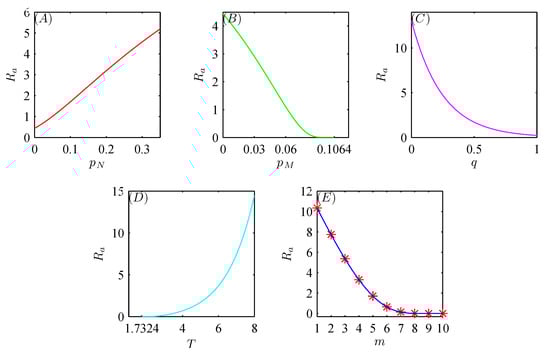
Figure 2. Simulations of the effects of $p_N$, $p_M$, q, T, and m on $R_a$. The baseline parameter values are fixed as follows: $D=0.08$, $b=1.5$, $a=0.6$, $K=10$, $\alpha =0.5$, $p_N=0.1$, $p_P=0.35$, $p_M=0.05$, $q=0.5$, $T=5$, and $m=5$.

According to Theorems 1 and 2, when $R_s<1$, $R_a<1$, and $R_s>1$, the pest-free periodic solution $(y^{\ast }\left(t\right),0)$ is locally asymptotically stable, globally attractive, and unstable, respectively (see Figure 3A).

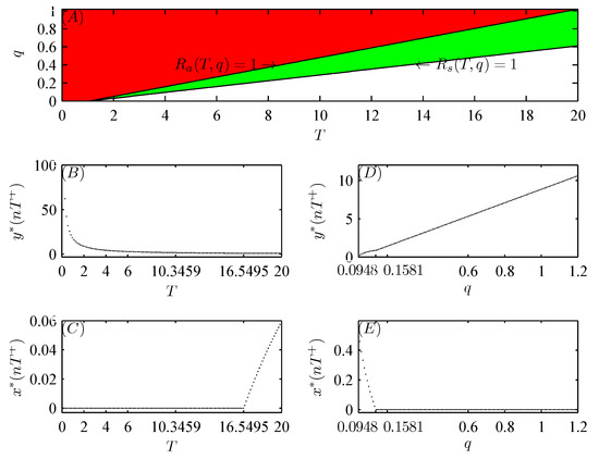
Figure 3. Bifurcation diagrams of system (52) with respect to T and q, where the other parameter values are fixed as follows: $D=0.08$, $\beta =0.19$, $b=1.5$, $a=0.4$, $K=1$, $\alpha =0.5$, $p_N=0.08$, $p_P=0.35$, $p_M=0.028$, and $m=3$. (A): Two-dimensional bifurcation diagram with respect to T and q, where the green, red, and white regions denotes the locally stable, globally stable, and unstable regions of the pest-free periodic solution $(y^{\ast }\left(t\right),0)$, respectively; (B,C): one-dimensional diagrams with respect to T, where $q=0.5$ and the initial values are $(0,{10}^6)$ and $(1.0277,{10}^{-10})$; (D,E): one-dimensional diagrams with respect to q, where $T=4$ and the initial values are $(0,{10}^6)$ and $(0.8369,{10}^{-10})$.

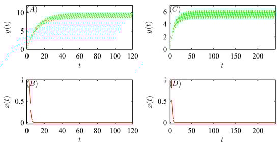
Figure 3B,C show that when $T<T_a=10.3459$, the global attractiveness of the pest-free periodic solution $(y^{\ast }\left(t\right),0)$ can be validated (see Figure 4A,B); however, when $T>T_b=16.5495$, the emergence of a pest-present solution leads to the loss of the local stability of the pest-free periodic solution, i.e., system (52) is permanent (see Figure 5A–C). Similar numerical analysis is suitable for the bifurcation of a pest-present periodic solution with respect to q (see Figure 3D,E and Figure 4C,D). In addition, Figure 5D–F confirm that when Corollary 1 holds, the global attractive pest-present periodic solution emerges.

Figure 4. Dynamic behaviors of system (52) with integrated pest management. (A,B): $q=0.5$, $T=2$; (C,D): $q=0.6$, $T=4$. The other parameters are identical to those in Figure 3, and the initial values are $(0,{10}^6)$.

Figure 5. Dynamic behaviors of system (52) with integrated pest management. (A–C): $q=0.5$, $T=17$, and the other parameters are identical to those in Figure 3; (D–F): the parameter values are fixed as follows: $D=0.4$, $\beta =0.16$, $b=1.5$, $a=1$, $K=1$, $\alpha =0.5$, $p_N=0.05$, $p_P=0.35$, $p_M=0$, $q=0.5$, $T=2$ and $m=3$. The initial values are (A–C) $(1.0277,{10}^{-10})$; (D–F) $({10}^{-12},{10}^{-12})$.

Furthermore, Figure 6 and Figure 7 show that model (52) exhibits more complex and interesting dynamic behaviors, including periodic doubling bifurcation, chaotic solutions, periodic adding\reducing, periodic windows, periodic halving bifurcation, and chaos crisis with increasing implementation period T and amount of released natural enemies q, respectively [32].

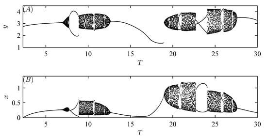
Figure 6. Bifurcation diagrams of system (52) with respect to parameter T. The other parameter values are fixed as follows: $D=0.2$, $\beta =0.91$, $b=2.04$, $a=1.5$, $K=3.5$, $\alpha =1$, $p_N=0.06$, $p_P=0.2$, $p_M=0.1$, $q=0.5$, $m=2$, and the initial value is $(2,1)$.

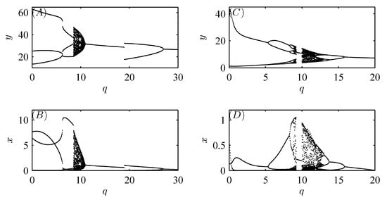
Figure 7. Bifurcation diagrams of system (52) with respect to parameter q. (A,B). $D=0.2$, $\beta =1.17$, $b=27.5$, $a=1.5$, $K=55$, $\alpha =1.3$, $p_N=0.06$, $p_P=0.3$, $p_M=0.1$, $T=12$, $m=2$, and the initial value is $(2,1)$; (C,D): $D=0.34$, $\beta =1.17$, $b=10$, $a=1.5$, $K=44$, $\alpha =1.3$, $p_N=0.06$, $p_P=0.7$, $p_M=0.1$, $T=11.25$, $m=2$, and the initial values is $(5,5)$.

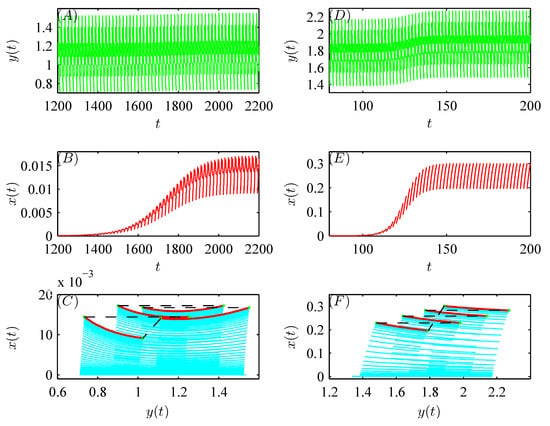
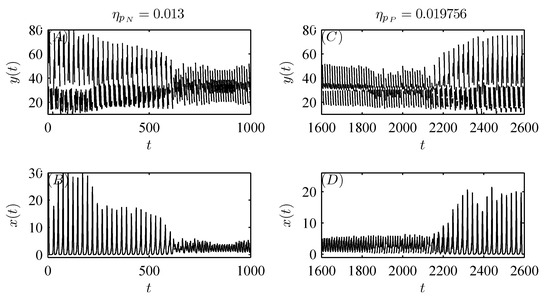
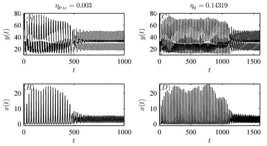
Moreover, random perturbations due to variations in the dosages applied or releases (migration) of natural enemies can also be taken into account with parameters $p_N$, $p_P$, $p_M$, and q. For example, when small random perturbations are introduced in one of the parameters $p_N$, $p_M$, and q, as shown in Figure 8, Figure 9A,B and Figure 10, the stable attractor with initial value $(9,6)$ can switch to another attractor with a smaller amplitude at a random time. Conversely, if a small random perturbation is introduced in parameter $p_P$, Figure 9C,D show that the stable attractor with initial value $(2,1)$ can switch to another attractor with a larger amplitude at a random time. Thus, different doses of pesticide application and natural enemy release (or migration) can influence the dynamics of the system (3).

Figure 8. Two coexisting attractors of system (52) with $q=16$ and the other parameters identical to those in Figure 7A,B. The initial values are (A,B) $(2,1)$; (C,D) $(9,6)$.

Figure 9. Attractors’ switch-like behaviors of system (52) with small random perturbations on parameters $p_N$ and $p_P$, i.e., ${\eta }_{p_N}=0.013$ and ${\eta }_{p_P}=0.019756$. The baseline parameters are identical to those in Figure 8, and the initial values are (A,B) $(9,6)$; (C,D) $(2,1)$.

Figure 10. Attractors’ switch-like behaviors of system (52) with small random perturbations on parameters $p_M$ and q, i.e., ${\eta }_{p_M}=0.003$ and ${\eta }_q=0.14319$. The baseline parameters are identical to those in Figure 8, and the initial values are $(9,6)$.

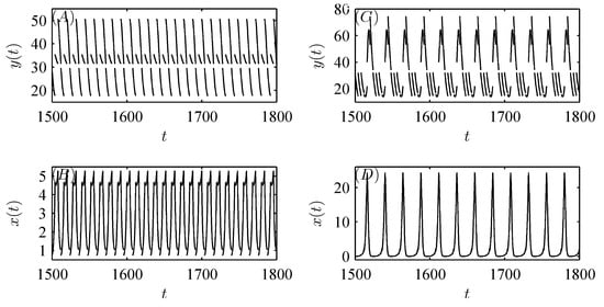
Moreover, Figure 11A shows that the pest population behaves in a “positive” fashion with pesticide spraying alone. As natural enemy release (or migration) is introduced to control pests, the pest population also oscillates in a periodic cycle but with a much smaller amplitude, revealing that the tendency of pests to become extinct becomes increasingly significant as m increases gradually (see Figure 11B,C). In particular, when m is sufficiently large, the pest population is eventually eradicated with integrated pest management (see Figure 11D). Thus, we demonstrate that integrated pest management is more effective than pesticide spraying alone.

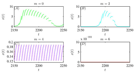
Figure 11. Dynamic behaviors of system (52) with integrated pest management. (A): $m=0$, $p_M=0$, $q=0$; (B): $m=2$; (C): $m=4$; (D): $m=6$. The other parameter values are fixed as follows: $D=0.08$, $\beta =0.16$, $b=1.5$, $a=0.6$, $K=10$, $\alpha =0.5$, $p_N=0.1$, $p_P=0.35$, $p_M=0.05$, $q=0.1$, $T=5$, and the initial value is $(2,1)$.

6. Discussion

In this study, we develop a predator–prey model with variation multiple pulse intervention effects to determine how chemical and biological control tactics affect pest control dynamics.

By employing the variational method, we determine the eigenvalues of the Jacobian matrix at the fixed point corresponding to the pest-free periodic solution. This fact is used to obtain the local stability threshold condition. A sufficient condition for the global attractiveness of the pest-free periodic solution is given as in (18). Moreover, the loss of local stability of the pest-free periodic solution results in the emergence of a pest-present periodic solution in the local neighborhood of the bifurcation point; furthermore, the permanence of system (3) is valid under certain conditions. Based on the techniques used in [33,34,35,36,37,38,39,40,41,42], the existence and global attractiveness of the pest-present periodic solution are analyzed by using Cauchy’s convergence principle under certain conditions, and a special case is obtained.

Our results demonstrate that the effectiveness of integrated pest management is crucial for pest prevention and resurgence. The numerical results presented in Section 5 indicate that $R_a$ is sensitive to small changes in several key parameters, such as $p_N$, $p_M$, q, T, and m. Furthermore, we perform two-parameter bifurcation analyses on the threshold values $R_s$ and $R_a$, which involve the local stability and global attractiveness of the pest-free periodic solution. Figure 3 shows the impacts of the period T and the amount q of natural enemies released on the behaviors of system (52).

Figure 6 and Figure 7 show that model (52) has several interesting dynamic behaviors, such as periodic doubling bifurcations, chaos, periodic adding\reducing, periodic windows, and periodic halving bifurcation. Moreover, the switch-like transitions between the two attractors reveal that both varying dosages of insecticide and the numbers of natural enemies released (or migrated) are crucial for pest control. In addition, further numerical simulations indicate that integrated pest management is more effective than pesticide spraying alone.

Compared with other relevant studies, the highlights of our study are as follows:

$\left(i\right)$ A continuous point can be viewed as a special impulsive point, i.e., the corresponding pulsed killing rate for the prey and predator populations, and the pulsed increment or migration rate of the natural enemies can be regarded as 0. Then, we propose model (3) to characterize all the possible situations of the implementation of the IPM strategy in reality. The traditional modeling approaches illustrated in [21,22,43,44] are special cases of our model.

$\left(ii\right)$ Due to the complexity of our modeling approach, it is difficult for us to prove the permanence of system (3) by using the traditional proof method demonstrated in [21,45]. Therefore, we prove the permanence of system (3) by constructing two uniform lower impulsive comparison systems on the interval $(t_3,+\infty )$, where (37) holds. If $\widehat{x}\left(t\right)$ is viewed as the second prey population, (39) and (40) indicate that the change rate of $x\left(t\right)$ is greater than that of $\widehat{x}\left(t\right)$; thus, $x\left(t\right)\ge \widehat{x}\left(t\right)$ holds within the interval $[{t^{\ast }}^{+},+\infty )$.

However, if we view $\tilde{x}\left(t\right)$ as the third prey population, (43) indicates that the change rate of $x\left(t\right)$ is greater than that of $\tilde{x}\left(t\right)$. Thus, when $\tilde{x}\left(t\right)$ jumps above the threshold line $x=m_0$ at time $t=(n_1+1)T+n_{2}T$, $x\left(t\right)$ also jumps above the threshold line $x=m_0$ at some $t_6\in ((n_1+1)T,(n_1+1)T+n_{2}T)$. Since the change rate of $\widehat{x}\left(t\right)$ is negative or the density of $\widehat{x}\left(t\right)$ decreases as $t\to +\infty$, it follows on the interval $(t^{\ast },t_6)$ that $x\left(t\right)>\widehat{x}((n_1+1)T+n_{2}T)$, which only depends on $m_0$.

In addition, the fact that $t=t^{\ast }$ and $t=t^{\ast \ast }$ are always viewed as impulsive times facilitates our proof. $\forall t\in ((n_1+1)T,t_6)$, it may hold that $x\left(t\right)<m_0$, $x\left(t\right)=m_0$ or $x\left(t\right)>m_0$.

$\left(iii\right)$ To date, the global attractiveness of the pest-present periodic solution of system (3) has not been addressed. Then, based on the permanence of system (3), we define a norm $V\left(t\right)$ with respect to the solution of system (3) and then construct an impulsive comparison system for $V\left(t\right)$. Similar to the proof of the contraction mapping principle, we prove the existence and global attractiveness of the pest-present periodic solution of system (3).

$\left(iv\right)$ According to the conclusion in [27], the bifurcation of the nontrivial periodic solution in [45,46,47,48,49] can be determined under certain conditions. However, the bifurcation of the pest-present periodic solution of system (3) cannot be handled in the same manner. Based on the implicit function theorem, we address this problem successfully. Compared to the following equation mentioned in [46,47]

$$2B\tilde{\tau }+Ca+{\displaystyle \frac{1}{a}}o(\tilde{\tau },a)({\tilde{\tau }}^2+a^2)=0,$$

the existence of the pest-present periodic solution is inferred from $\widehat{f}(T,c_p)=0$ more rigorously.

As T gradually increases in interval $[T_b,T_b+\overline{\delta })$, the IPM strategy is implemented less frequently so as not to control the pests. Then, a pest-present periodic solution emerges. Biologically speaking, during the evolution of T, the pest-free periodic solution becomes unstable; intuitively, to maintain the ecological/systematic balance, both the prey and predator populations should eventually stabilize around a pest-present periodic solution. Given the numerical results in Figure 3, we hypothesize that the pest-present periodic solution obtained above is locally stable. We plan to investigate the stability of the pest-free solution in our future research.

References

- Li, Z. A disease-specific screening-level modeling approach for assessing the cancer risks of pesticide mixtures. Chemosphere 2022, 286, 131811. [Google Scholar] [CrossRef] [PubMed]
- Josea, S.A.; Raja, R.; Zhu, Q.; Alzabut, J.; Niezabitowski, M.; Balas, V.E. An integrated eco-epidemiological plant pest natural enemy differential equation model with various impulsive strategies. Math. Probl. Eng. 2022, 2022, 4780680. [Google Scholar] [CrossRef]
- Chowdhury, J.; Al Basir, F.; Cao, X.; Kumar Roy, P. Integrated pest management for Jatropha Carcus plant: An impulsive control approach. Math. Methods Appl. Sci. 2021, 1–16. [Google Scholar] [CrossRef]
- Hou, X.; Fu, J.; Cheng, H. Sensitivity analysis of pesticide dose on predator-prey system with a prey refuge. J. Appl. Anal. Comput. 2022, 12, 270–293. [Google Scholar] [CrossRef]
- Al Basir, F.; Chowdhury, J.; Das, S.; Ray, S. Combined impact of predatory insects and bio-pesticide over pest population: Impulsive model-based study. Energy Ecol. Environ. 2022, 7, 173–185. [Google Scholar] [CrossRef]
- Hu, J.; Liu, J.; Yuen, P.W.; Li, F.; Deng, L. Modelling of a seasonally perturbed competitive three species impulsive system. Math. Biosci. Eng. 2022, 19, 3223–3241. [Google Scholar] [CrossRef]
- Joseb, S.A.; Ramachandran, R.; Cao, J.; Alzabut, J.; Niezabitowski, M.; Balas, V.E. Stability analysis and comparative study on different eco-epidemiological models: Stage structure for prey and predator concerning impulsive control. Optim. Contr. Appl. Methods 2022, 43, 842–866. [Google Scholar] [CrossRef]
- Liu, J.; Hu, J.; Yuen, P.; Li, F. A seasonally competitive M-prey and N-predator impulsive system modeled by general functional response for integrated pest management. Mathematics 2022, 10, 2687. [Google Scholar] [CrossRef]
- Dai, C. Dynamic complexity in a prey-predator model with state-dependent impulsive control strategy. Complexity 2020, 2020, 1614894. [Google Scholar] [CrossRef]
- Tian, Y.; Tang, S. Dynamics of a density-dependent predator-prey biological system with nonlinear impulsive control. Math. Biosci. Eng. 2021, 18, 7318–7343. [Google Scholar] [CrossRef]
- Su, Y.; Zhang, T. Global dynamics of a predator-prey model with fear effect and impulsive state feedback control. Mathematics 2022, 10, 1229. [Google Scholar] [CrossRef]
- Zhu, X.; Wang, H.; Ouyang, Z. The state-dependent impulsive control for a general predator-prey model. J. Biol. Dynam. 2022, 16, 354–372. [Google Scholar] [CrossRef]
- Li, Y.F.; Zhu, C.Z.; Liu, Y.W. Dynamic analysis of a predator-prey model with state-dependent impulsive effects. Chin. Q. J. Math. 2023, 38, 1–19. [Google Scholar]
- Yu, X.; Huang, M. Dynamics of a Gilpin-Ayala predator-prey system with state feedback weighted harvest strategy. AIMS Math. 2023, 8, 26968–26990. [Google Scholar] [CrossRef]
- Wu, L.; Xiang, Z. Dynamic analysis of a predator-prey impulse model with action threshold depending on the density of the predator and its rate of change. AIMS Math. 2024, 9, 10659–10678. [Google Scholar] [CrossRef]
- Cheng, H.; Zhang, X.; Zhang, T.; Fu, J. Dynamics analysis of a nonlinear controlled predator-prey model with complex Poincaré map. Nonlinear Anal. Model. Control 2024, 29, 466–487. [Google Scholar] [CrossRef]
- Al Basir, F.; Chowdhury, J.; Torres, D.F. Dynamics of a double-impulsive control model of integrated pest management using perturbation methods and Floquet theory. Axioms 2023, 12, 391. [Google Scholar] [CrossRef]
- Diz-Pita, É.; Otero-Espinar, M.V. Predator-prey models: A review of some recent advances. Mathematics 2021, 9, 1783. [Google Scholar] [CrossRef]
- Wang, S.; Yu, H. Stability and bifurcation analysis of the Bazykins predator-prey ecosystem with Holling type II functional response. Math. Biosci. Eng. 2021, 18, 7877–7918. [Google Scholar] [CrossRef]
- Feketa, P.; Klinshov, V.; Lücken, L. A survey on the modeling of hybrid behaviors: How to account for impulsive jumps properly. Commun. Nonlinear Sci. 2021, 103, 105955. [Google Scholar] [CrossRef]
- Liu, J.; Hu, J.; Yuen, P. Extinction and permanence of the predator-prey system with general functional response and impulsive control. Appl. Math. Model. 2020, 88, 55–67. [Google Scholar] [CrossRef]
- Zhao, Z.; Pang, L.; Li, Q. Analysis of a hybrid impulsive tumor-immune model with immunotherapy and chemotherapy. Chaos Solitons Fract. 2021, 144, 110617. [Google Scholar] [CrossRef]
- Liu, X.; Chen, L. Global dynamics of the periodic logistic system with periodic impulsive perturbations. J. Math. Anal. Appl. 2004, 289, 279–291. [Google Scholar] [CrossRef]
- Jiao, J.; Quan, Q.; Dai, X. Dynamics of a new impulsive predator-prey model with predator population seasonally large-scale migration. Appl. Math. Lett. 2022, 132, 108096. [Google Scholar] [CrossRef]
- Dai, X.; Jiao, H.; Jiao, J.; Quan, Q. Survival analysis of a predator-prey model with seasonal migration of prey populations between breeding and non-breeding regions. Mathematics 2023, 11, 3838. [Google Scholar] [CrossRef]
- Quan, Q.; Dai, X.; Jiao, J. Dynamics of a predator-prey model with impulsive diffusion and transient/nontransient impulsive harvesting. Mathematics 2023, 11, 3254. [Google Scholar] [CrossRef]
- Lakmeche, A. Birfurcation of non-trivial periodic solutions of impulsive differential equations arising chemotherapeutic treatment. Dynam. Contin. Discret. Impuls. 2000, 7, 265–287. [Google Scholar]
- Bainov, D.; Simeonov, P. Impulsive Differential Equations: Periodic Solutions and Applications; Longman Scientific & Technical Press: New York, NY, USA, 1993. [Google Scholar]
- Wang, G.; Yi, M.; Tang, S. Dynamics of an antitumour model with pulsed radioimmunotherapy. Comput. Math. Methods Med. 2022, 2022, 4692772. [Google Scholar] [CrossRef]
- Wang, L.; She, A.; Xie, Y. The dynamics analysis of Gompertz virus disease model under impulsive control. Sci. Rep. 2023, 13, 10180. [Google Scholar] [CrossRef]
- Wang, G.; Zou, X. Qualitative analysis of critical transitions in complex disease propagation from a dynamical systems perspective. Int. J. Bifurcat. Chaos 2016, 26, 1650239. [Google Scholar] [CrossRef]
- Guo, J.; Liu, X.; Yan, P. Dynamic analysis of impulsive differential chaotic system and its application in image encryption. Mathematics 2023, 11, 4835. [Google Scholar] [CrossRef]
- Tan, R.; Liu, Z.; Cheke, R.A. Periodicity and stability in a single-species model governed by impulsive differential equation. Appl. Math. Model. 2012, 36, 1085–1094. [Google Scholar] [CrossRef]
- Li, X.; Bohner, M.; Wang, C.K. Impulsive differential equations: Periodic solutions and applications. Automatica 2015, 52, 173–178. [Google Scholar] [CrossRef]
- Tamen, A.T.; Dumont, Y.; Tewa, J.J.; Bowong, S.; Couteron, P. A minimalistic model of tree-grass interactions using impulsive differential equations and non-linear feedback functions of grass biomass onto fire-induced tree mortality. Math. Comput. Simul. 2017, 133, 265–297. [Google Scholar] [CrossRef]
- Lin, Q.; Xie, X.; Chen, F.; Lin, Q. Dynamical analysis of a logistic model with impulsive Holling type-II harvesting. Adv. Differ. Equ. 2018, 2018, 112. [Google Scholar] [CrossRef]
- Sun, L.; Zhu, H.; Ding, Y. Impulsive control for persistence and periodicity of logistic systems. Math. Comput. Simul. 2020, 171, 294–305. [Google Scholar] [CrossRef]
- Boudaoui, A.; Mebarki, K.; Shatanawi, W.; Abodayeh, K. Solution of some impulsive differential equations via coupled fixed point. Symmetry 2021, 13, 501. [Google Scholar] [CrossRef]
- Duque, C.; Uzcátegui, J.; Ruiz, B.; Pérez, M. Attractive periodic solutions of a discrete Holling-Tanner predator-prey model with impulsive effect. Bull. Comput. Appl. Math. 2021, 8, 49–63. [Google Scholar]
- Yan, Y.; Wang, K.; Gui, Z. Periodic solution of impulsive predator-prey model with stage structure for the prey undercrowding effect. J. Phys. Conf. Ser. 2021, 1903, 012032. [Google Scholar] [CrossRef]
- Duque, C.; Diestra, J.L.H. Positive periodic solutions of a discrete ratio-dependent predator-prey model with impulsive effects. Rev. Union Math. Argent. 2022, 63, 137–151. [Google Scholar] [CrossRef]
- Shukla, A.; Vijayakumar, V.; Nisar, K.S.; Singh, A.K.; Udhayakumar, R.; Botmart, T.; Albalawi, W.; Mahmoud, M. An analysis on approximate controllability of semilinear control systems with impulsive effects. Alex. Eng. J. 2022, 61, 12293–12299. [Google Scholar] [CrossRef]
- Li, C.; Feng, X.; Wang, Y.; Wang, X. Complex dynamics of Beddington-DeAngelis-Type predator-prey model with nonlinear impulsive control. Complexity 2020, 2020, 8829235. [Google Scholar] [CrossRef]
- Sirisubtawee, S.; Khansai, N.; Charoenloedmongkhon, A. Investigation on dynamics of an impulsive predator-prey system with generalized Holling type IV functional response and anti-predator behavior. Adv. Differ. Equ. 2021, 2021, 160. [Google Scholar] [CrossRef]
- Wang, L.J.; Xie, Y.X.; Deng, Q.C. The dynamic behaviors of a new impulsive predator prey model with impulsive control at different fixed moments. Kybernetika 2018, 54, 522–541. [Google Scholar] [CrossRef]
- Li, C.; Tang, S. Analyzing a generalized pest-natural enemy model with nonlinear impulsive control. Open Math. 2018, 16, 1390–1411. [Google Scholar] [CrossRef]
- Li, C.; Tang, S.; Cheke, R.A. Complex dynamics and coexistence of period-doubling and period-halving bifurcations in an integrated pest management model with nonlinear impulsive control. Adv. Differ. Equ. 2020, 2020, 514. [Google Scholar] [CrossRef]
- Li, Z.; Yang, X.; Fu, S. Dynamical behavior of a predator-prey system incorporating a prey refuge with impulse effect. Complexity 2022, 2022, 2422923. [Google Scholar] [CrossRef]
- Prathumwan, D.; Trachoo, K.; Maiaugree, W.; Chaiya, I. Preventing extinction in Rastrelliger brachysoma using an impulsive mathematical model. AIMS Math. 2022, 7, 1–24. [Google Scholar] [CrossRef]
Disclaimer/Publisher’s Note: The statements, opinions and data contained in all publications are solely those of the individual author(s) and contributor(s) and not of MDPI and/or the editor(s). MDPI and/or the editor(s) disclaim responsibility for any injury to people or property resulting from any ideas, methods, instructions or products referred to in the content. |
© 2025 by the authors. Licensee MDPI, Basel, Switzerland. This article is an open access article distributed under the terms and conditions of the Creative Commons Attribution (CC BY) license (https://creativecommons.org/licenses/by/4.0/).