Article

Tackling Blind Spot Challenges in Metaheuristics Algorithms Through Exploration and Exploitation

1
Faculty of Electrical Engineering and Computer Science, University of Maribor, Koroška cesta 46, 2000 Maribor, Slovenia
2
Department of Applied Mathematics, Florida Polytechnic University, 4700 Research Way, Lakeland, FL 33805, USA
*
Author to whom correspondence should be addressed.
Mathematics 2025, 13(10), 1580; https://doi.org/10.3390/math13101580
Submission received: 10 April 2025 / Revised: 8 May 2025 / Accepted: 9 May 2025 / Published: 11 May 2025
(This article belongs to the Section E1: Mathematics and Computer Science)

Abstract

:
This paper defines blind spots in continuous optimization problems as global optima that are inherently difficult to locate due to deceptive, misleading, or barren regions in the fitness landscape. Such regions can mislead the search process, trap metaheuristic algorithms (MAs) in local optima, or hide global optima in isolated regions, making effective exploration particularly challenging. To address the issue of premature convergence caused by blind spots, we propose LTMA+ (Long-Term Memory Assistance Plus), a novel meta-approach that enhances the search capabilities of MAs. LTMA+ extends the original Long-Term Memory Assistance (LTMA) by introducing strategies for handling duplicate evaluations, shifting the search away from over-exploited regions and dynamically toward unexplored areas and thereby improving global search efficiency and robustness. We introduce the Blind Spot benchmark, a specialized test suite designed to expose weaknesses in exploration by embedding global optima within deceptive fitness landscapes. To validate LTMA+, we benchmark it against a diverse set of MAs selected from the EARS framework, chosen for their different exploration mechanisms and relevance to continuous optimization problems. The tested MAs include ABC, LSHADE, jDElscop, and the more recent GAOA and MRFO. The experimental results show that LTMA+ improves the success rates for all the tested MAs on the Blind Spot benchmark statistically significantly, enhances solution accuracy, and accelerates convergence to the global optima compared to standard MAs with and without LTMA. Furthermore, evaluations on standard benchmarks without blind spots, such as CEC’15 and the soil model problem, confirm that LTMA+ maintains strong optimization performance without introducing significant computational overhead.

1. Introduction

Computer optimization is a key area of computational science that focuses on finding optimal solutions in complex problem spaces. Its applications span disciplines such as computer science, engineering, economics, and biology, supporting advancements in system design, resource allocation, and predictive modeling. Metaheuristic algorithms (MAs), a class of techniques inspired by natural processes, are central to this field due to their stochastic nature, which enables the exploration of diverse solutions to find near-optimal outcomes [1]. The comparison of different MAs is verified through experiments on different benchmarks and problems [2]. Although the benchmarks are adapted to measure the efficiency and robustness of the algorithms and are updated regularly, this can lead to the overfitting of the MAs’ development to the problems used for the comparison of the algorithms [3]. The unpredictability of various computational models and the human inclination toward certainty, as described by Nassim Nicholas Taleb in his books The Black Swan: The Impact of the Highly Improbable [4] and Antifragile [5], highlight the limitations of traditional predictive approaches. From stock market crashes and the collapse of empires to smaller anomalies—such as the triple flooding of a stream within 20 years, despite its bed being designed for 400-year flood events—these events underscore the antifragility of systems [6]. This perspective motivated us to explore the robustness of MAs, particularly for optimization problems with deceptive regions in their fitness landscapes. The bare minimum baseline for any optimization algorithm’s average performance on most problems (excluding highly stochastic or noisy problems) should surpass that of the random search (RS) algorithm. If it does not, the algorithm is either ineffective or fundamentally flawed. What we truly seek is the algorithm’s ability to thrive under stress, uncertainty, and challenges, improving its performance over time. A prime example in optimization is the use of self-adaptive control parameters, which enable the algorithm to adjust and enhance its behavior dynamically in response to the problem’s complexity [7,8,9]. By applying the LTMA meta-level approach to detect duplicate solutions and quantify population diversity [10], we introduce a novel diversity-guided adaptation mechanism with a memory-based archive of unique non-revisited solutions, enabling dynamic adjustment of MAs’ exploration mechanisms based on the frequency of duplicates and enhancing robustness against premature convergence in local optima.
The main contributions of this paper are as follows:
  • The development of Blind Spot, a novel benchmark problem crafted to expose vulnerabilities in existing algorithms.
  • The introduction of LTMA+, a meta-approach integrating diverse strategies to improve the robustness of MAs.
  • An empirical evaluation validating LTMA+’s effectiveness in enhancing algorithmic robustness across optimization tasks.
Section 2 provides a brief overview of the concepts of exploration and exploitation. In Section 3, we introduce a benchmark problem called blind spot, and we present unexpected cases where RS outperformed MAs. This outcome serves as a clear indication that the selected algorithms lacked robustness on the Blind Spot benchmark. In Section 4, we propose a novel meta-approach, LTMA+, designed to enhance the robustness of optimization algorithms. In Section 5, we present the experimental results, while, in Section 6 and Section 7, we provide a detailed discussion and conclude the paper, respectively. The paper includes an Appendix composed of seven sections, providing additional results, experiments, and analyses to support the study.

2. Related Work

MAs are a class of optimization algorithms inspired by the process of natural evolution, whose primary goal is the survival of the fittest [11,12,13]. They typically incorporate elements such as randomness, a population of candidate solutions, and mechanisms to search around promising solution candidates. The optimization process is generally iterative and continues until a stopping criterion is met, such as a time limit, a maximum number of evaluations, or another predefined condition [14,15]. The main objective of MAs is to find the optimal solution to a given problem by evolving a population of candidate solutions iteratively. This process relies on two fundamental components: exploration and exploitation of the search space [16]. Exploration refers to the search for new solutions across the unexplored regions, while exploitation focuses on refining and improving the previously visited solutions. Striking the right balance between exploration and exploitation is critical to the success of MAs [17,18,19]. Within the broader category, MAs represent high-level strategies that guide the search process [20]. Recent studies have highlighted their effectiveness in areas like real-world engineering design [21], unrelated-parallel-machine scheduling [22], multi-objective-optimization problems [23], and emerging fields such as swarm intelligence and bio-inspired computing [16,24]. More recently, MAs have advanced through hybridization techniques and applications in dynamic and uncertain environments [25,26]. Modern MAs are designed to be flexible and adaptable, making them suitable for a wide range of optimization problems. However, most MAs require the tuning of control parameters, which can influence their efficiency and effectiveness significantly.
To evaluate the general performance of MAs, researchers use benchmark problems designed to assess algorithm capabilities across diverse optimization challenges. These benchmarks include unimodal, multimodal, and composite functions, each presenting unique difficulties such as deceptive optima and high dimensionality [2]. The most popular benchmarks are the CEC Benchmark Suites [27], Black-Box Optimization Benchmarking (BBOB) [28], International Student Competition in Structural Optimization (ISCSO) [29], and a collection of Classical Benchmark Functions, including Sphere, Ackley, and Schwefel, which are often integrated into the aforementioned suites. These benchmarks are used widely in the research community to compare the performance of different MAs and to identify their strengths and weaknesses. However, it is important to note that the choice of benchmark problems can influence the perceived performance of an algorithm significantly. This has led to concerns about overfitting, where the algorithms are tailored to perform well on specific benchmarks but may not generalize effectively to other problem types [3].
The term “blind spot problem” in the optimization community often describes specific challenges, such as positioning radar antennas or cameras to maximize coverage [30,31,32]. In the paper “Breeding Machine Translations”, blind spots refer to weaknesses in automated evaluation metrics [33]. Similarly, in “Evolutionary-Algorithm-Based Strategy for Computer-Assisted Structure Elucidation”, blind spots are regions in the solution space where the correct structure might be overlooked [34]. With an approach closer to our usage, some authors define blind spots as regions in the search space that an algorithm may skip due to linear steps during exploitation [35]. In reinforcement learning, the term describes mismatches between a simulator’s state representation and real-world conditions, leading to blind spots [36]. In this paper, for continuous optimization problems, we define blind spots as optima that are inherently difficult to locate. The challenge stems from the problem’s fitness landscape, which can influence the search process directly by creating local optima that trap algorithms or guide them toward the global optimum through gradually changing local optima, as seen in the Ackley function. Certain landscapes can also be misleading or deceptive, directing search processes toward suboptimal regions [37,38]. Another difficulty arises in barren plateaus, where gradients vanish exponentially with the problem size, hindering progress [39,40,41]. It becomes particularly challenging when the global optimum lies in a region independent of its surroundings. Such a region represents a blind spot, a part of the search space where the objective function contains an optimum that is especially hard to identify. Defining the blind spot problem is crucial for understanding exploration challenges in algorithm optimization. One might ask the following: why not use established problems like Easom or Foxholes? These problems are insufficiently deceptive for our purposes (Appendix A) [14].
As computational power has advanced rapidly, we have observed an underutilization of memory during optimization processes. This issue has often been overlooked, from the early days of 640 KB memory to today’s 64 GB systems. In 2019, we introduced a meta-approach titled “Long-Term Memory Assistance for Evolutionary Algorithms” [10], which leverages memory during optimization to avoid redundant evaluations of previously explored solutions, known as duplicates. This is particularly significant, as solution evaluation is often the most computationally expensive part of optimization. The study [10] revealed a prevalence of duplicate solutions generated around the best-known solutions—a phenomenon often referred to as stagnation. Duplicates are identified when the genotypes x 1 and x 2 satisfy x 1 i = x 2 i for all i { 1 , , n } , where n is the problem dimension. In Java-based experiments, double-value precision (Pr) was limited to three, six, or nine decimal places for real-world optimization problems. LTMA achieved a ≥10% speedup on low computational cost problems, and a ≥59% speedup in a soil model optimization problem where the Artificial Bee Colony (ABC) algorithm generated 35% duplicates, mitigating stagnation around the known optima [10].
Our experiments aimed to explore blind spots, such as underexplored regions, in the optimization process of MAs, rather than compare their superiority. Selecting appropriate metaheuristic algorithms is crucial, as over 500 distinct algorithms had been documented by 2023 [42]. State-of-the-art metaheuristic algorithms are typically adaptive or self-adaptive, making them versatile for diverse optimization challenges. We chose metaheuristic algorithms for our experiments based on their adaptability, implementation within the EARS framework (which includes over 60 algorithms) [43], and recent advancements in the field. To ensure a focused study, we limited our selection to five algorithms. These algorithms or their variants have consistently demonstrated strong performance across diverse benchmark problems [44,45,46].
For the experiments, we selected adaptive, self-adaptive, and more recent MAs from the EARS framework [43], including Artificial Bee Colony (ABC), self-adaptive Differential Evolution (jDElscop) with dynamically encoded parameters and strategies [47], Linear Population Size Reduction Success-History Based Adaptive Differential Evolution (LSHADE) for balanced exploration and exploitation [48], the Gazelle Optimization Algorithm (GAOA) [49], and the Manta Ray Foraging Optimization (MRFO) [50]. A simple RS was included as a separate algorithm that samples solutions randomly in the search space without any specific optimization strategy. It serves as a reference point to evaluate the performance of the other algorithms.

3. The Blind Spot Benchmark

To analyze blind spots’ impact systematically, we define the blind spot problem for three classical optimization problems of increasing difficulty, serving as benchmarks to illustrate their effect on the selected MAs. For each problem, we will define the size of the blind spot.
The blind spot size we define as the percentage of the search space in a single dimension occupied by the blind spot. For example, if the search space is [ 100 , 100 ] and the blind spot spans [ 95 , 85 ] , it covers p = 0.05 % of the search space.
This definition seems intuitive for any number of dimensions. However, the blind spot’s size relative to the entire search space decreases exponentially as the dimensionality increases. To illustrate this, consider a search space where the blind spot’s probability remains constant across all dimensions (see Figure 1). Humans often struggle to visualize how small the blind spot becomes in higher dimensions.
The probability of finding the blind spot is p n , where n is the problem’s dimension. Since its location is independent of the fitness landscape, the likelihood of an MA discovering it is extremely low. In our experiments, we used a blind spot size of 0.05 % per dimension, with n ranging from 2 to 5. To assess algorithm robustness in higher dimensions, we recommend increasing the blind spot size or the number of blind spots.

3.1. Sphere Blind Spot Problem (Easy)

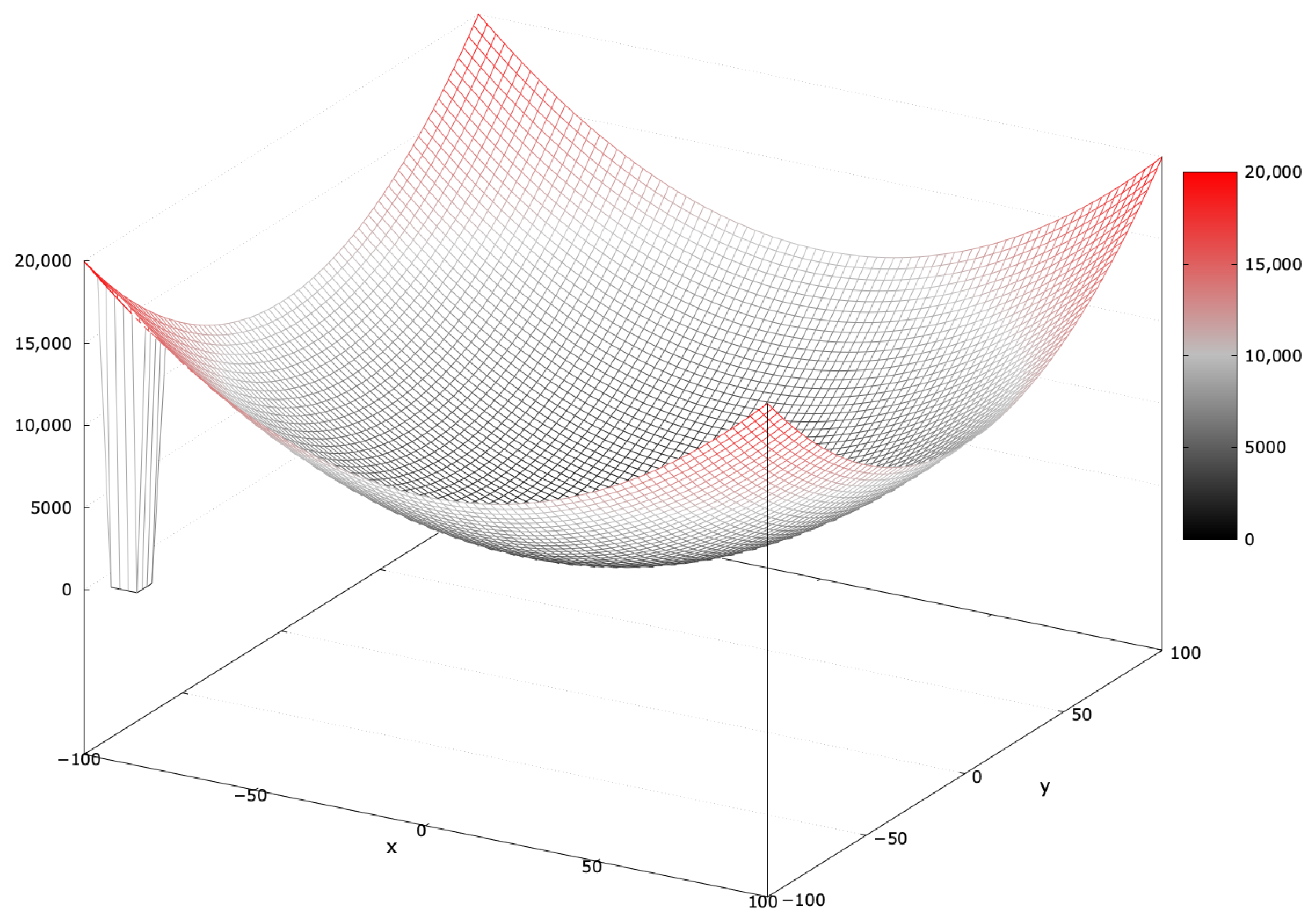
The basic Sphere function is unimodal with a single basin of attraction, making it a simple global optimization problem without local optima [51]. Introducing a blind spot covering 0.05 % of the search interval (denoted as SphereBS) transforms the global optimum into a local one, misleading the search process (see Figure 2).
Equation (1) defines the SphereBS minimization problem:
f ( x ) = i = 1 n x i 2 , if x i [ 100 , 100 ] for all i = 1 , , n and at least one x i [ 95 , 85 ] , 1 , if x i [ 95 , 85 ] for all i = 1 , , n .
The global optimum has a fitness value of 1 . The SphereBS function provides insight into an algorithm’s basic exploitation behavior.
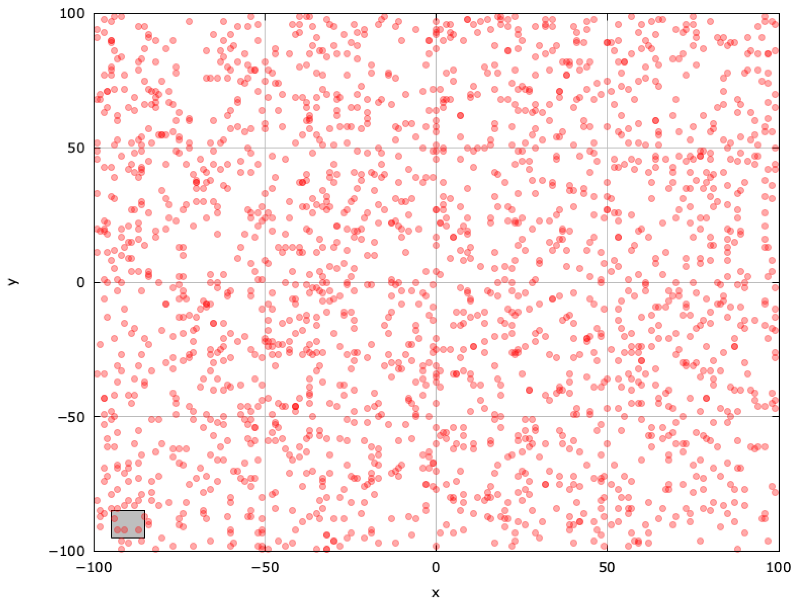
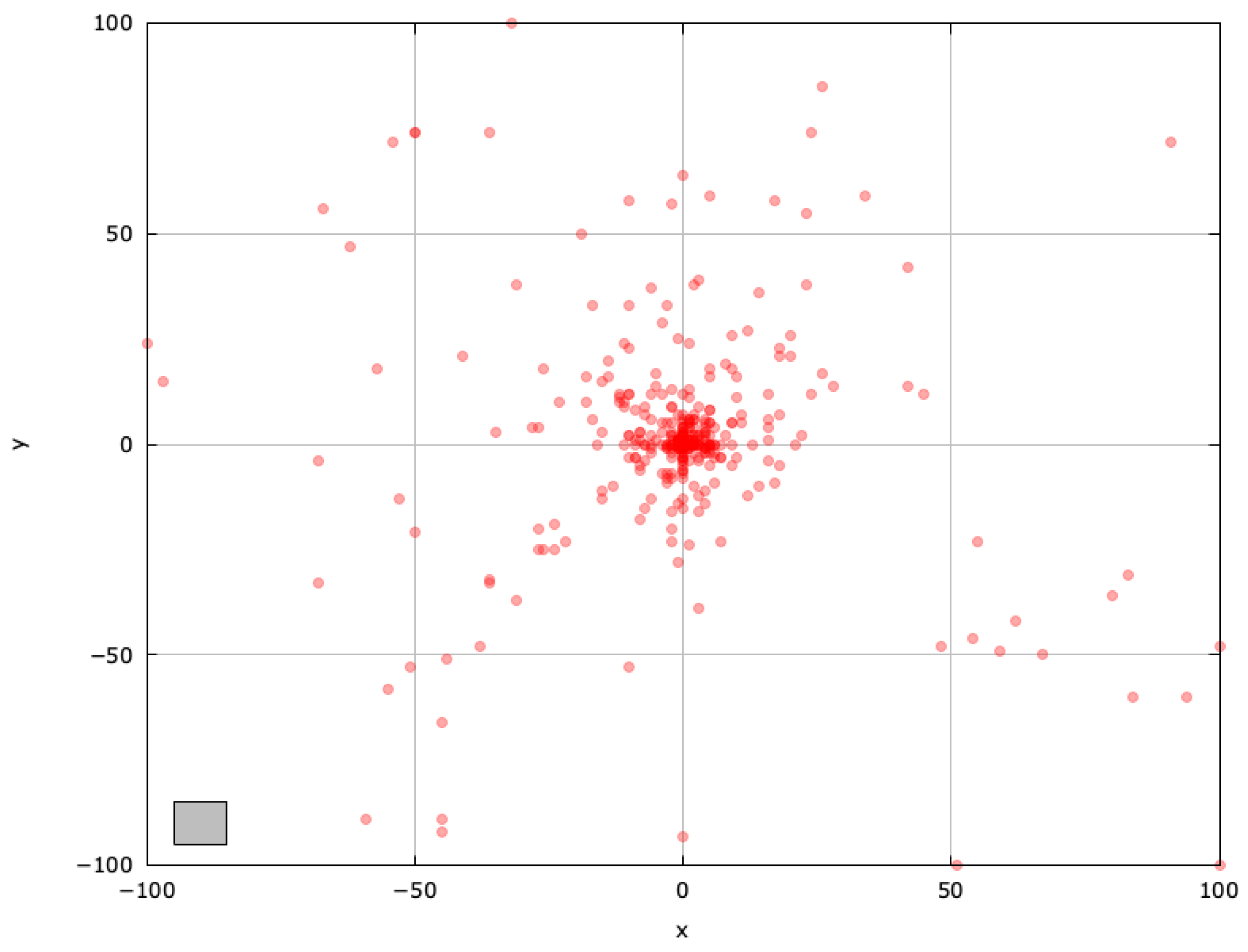
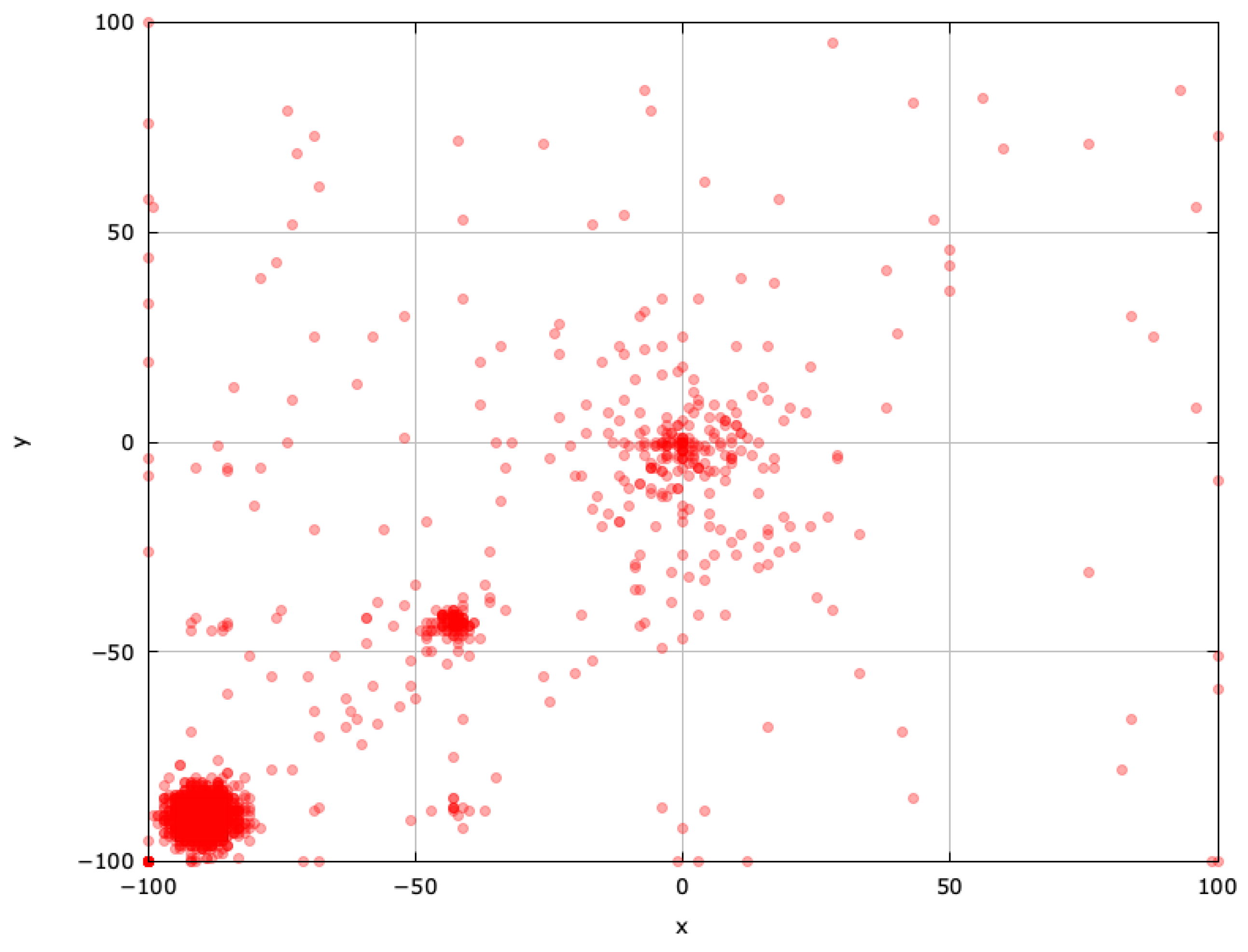
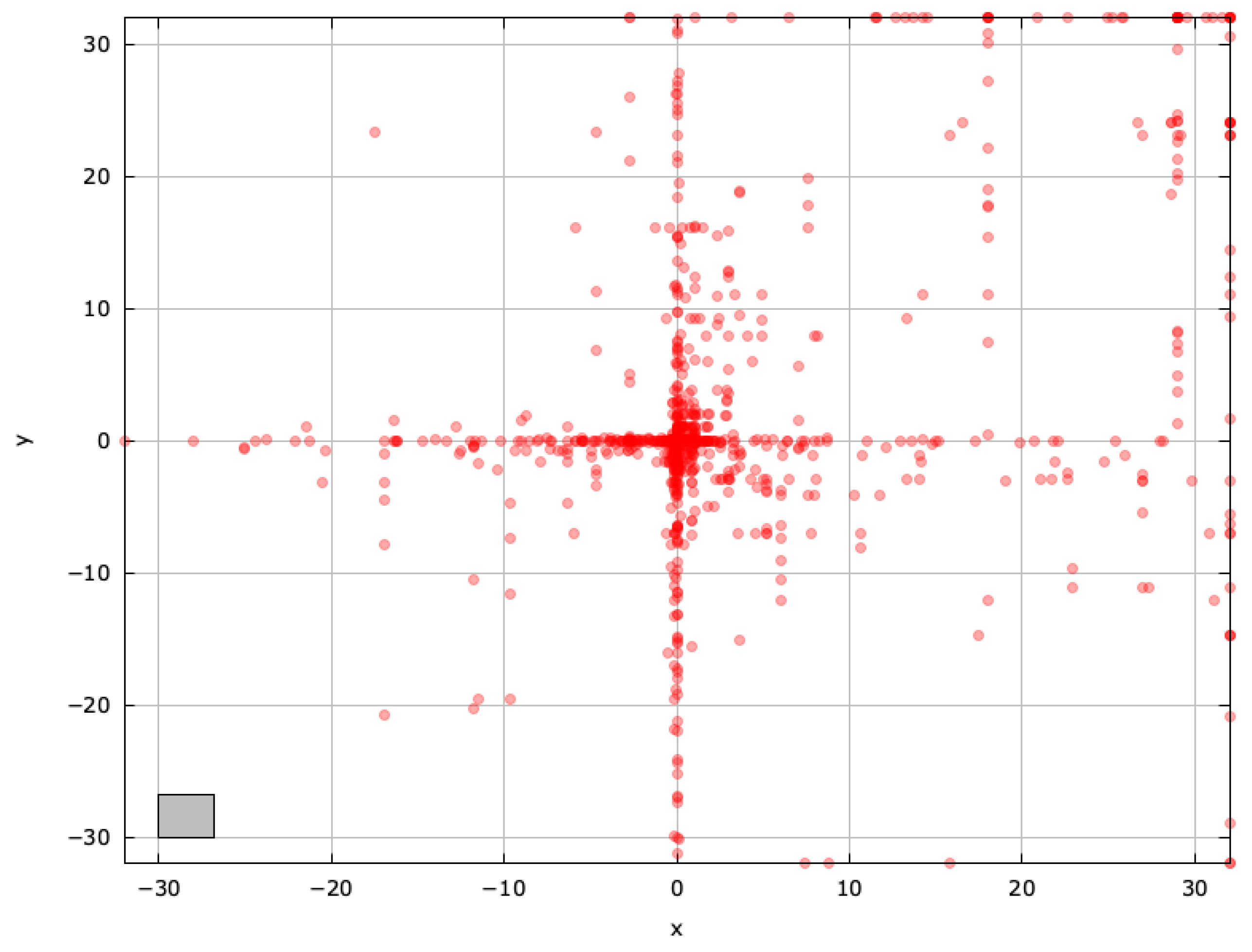
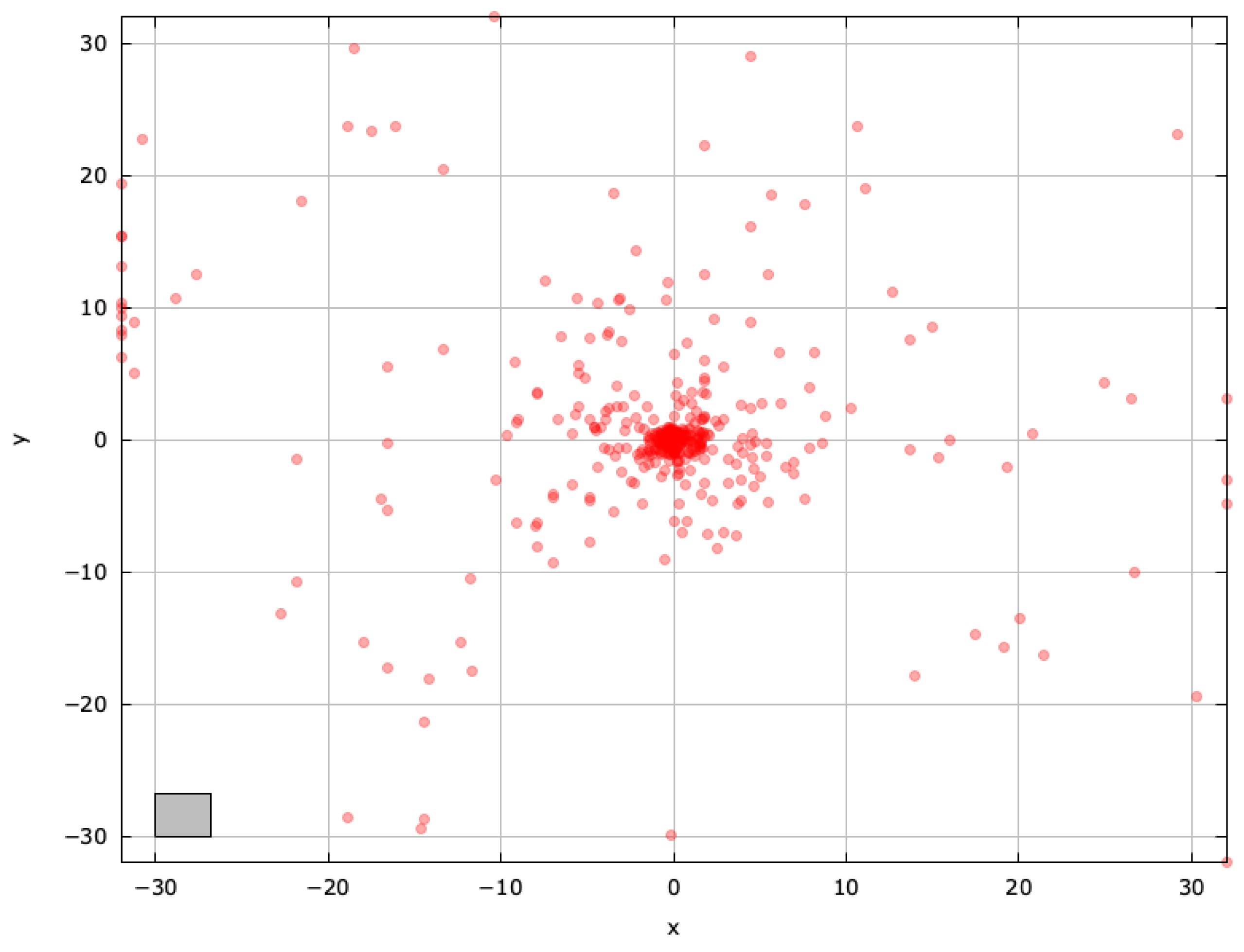
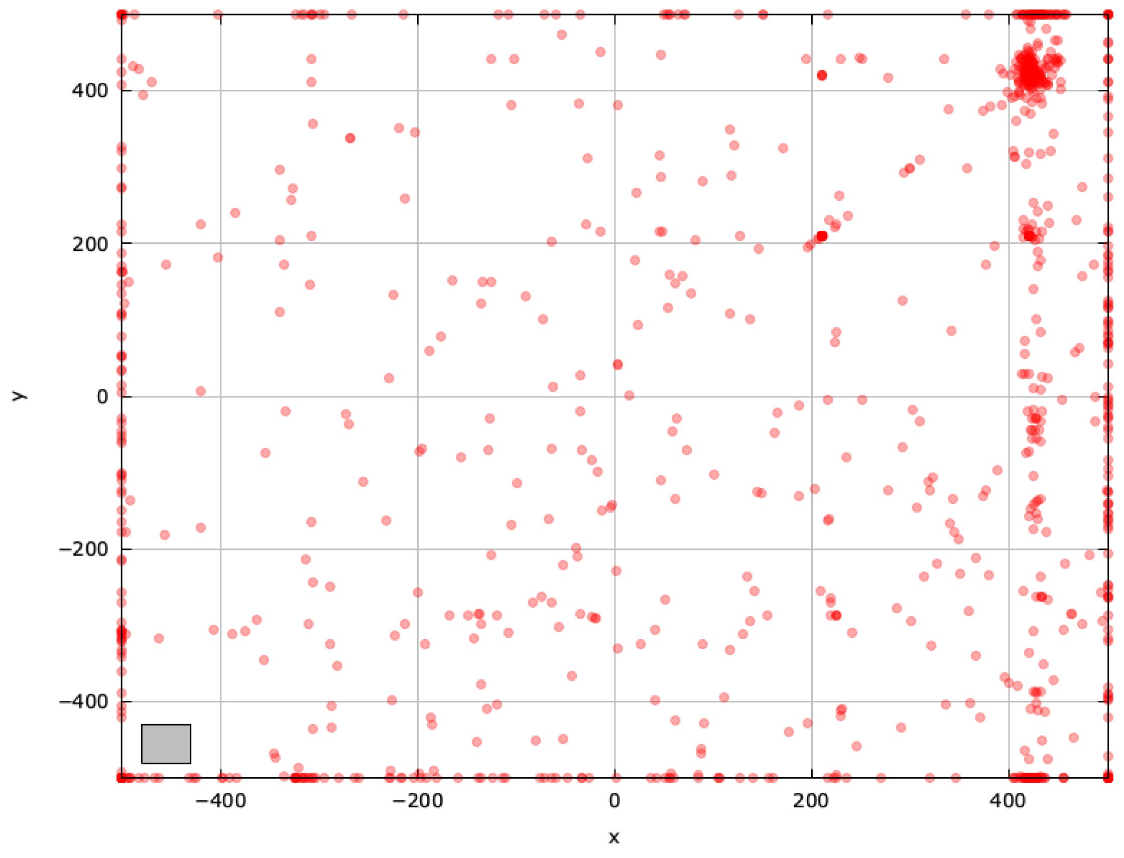
Every MA navigates the search space differently, with success hinging on balancing exploration and exploitation. Visualizing the 2D search space—representing each evaluated solution as a point—helps clarify these mechanics. Greater coverage typically indicates more diverse exploration.
To understand blind spots better and identify regions for improvement, we analyzed the search space explored with the MAs. For a single run of each selected algorithm, we used a population size of pop_size = 20 , n = 2 and a stopping criterion of M a x F E s = 2000 (maximum function evaluations). The results are shown in Figure 3, Figure 4, Figure 5, Figure 6, Figure 7, Figure 8 and Figure 9, with the blind spot highlighted with a gray rectangle.
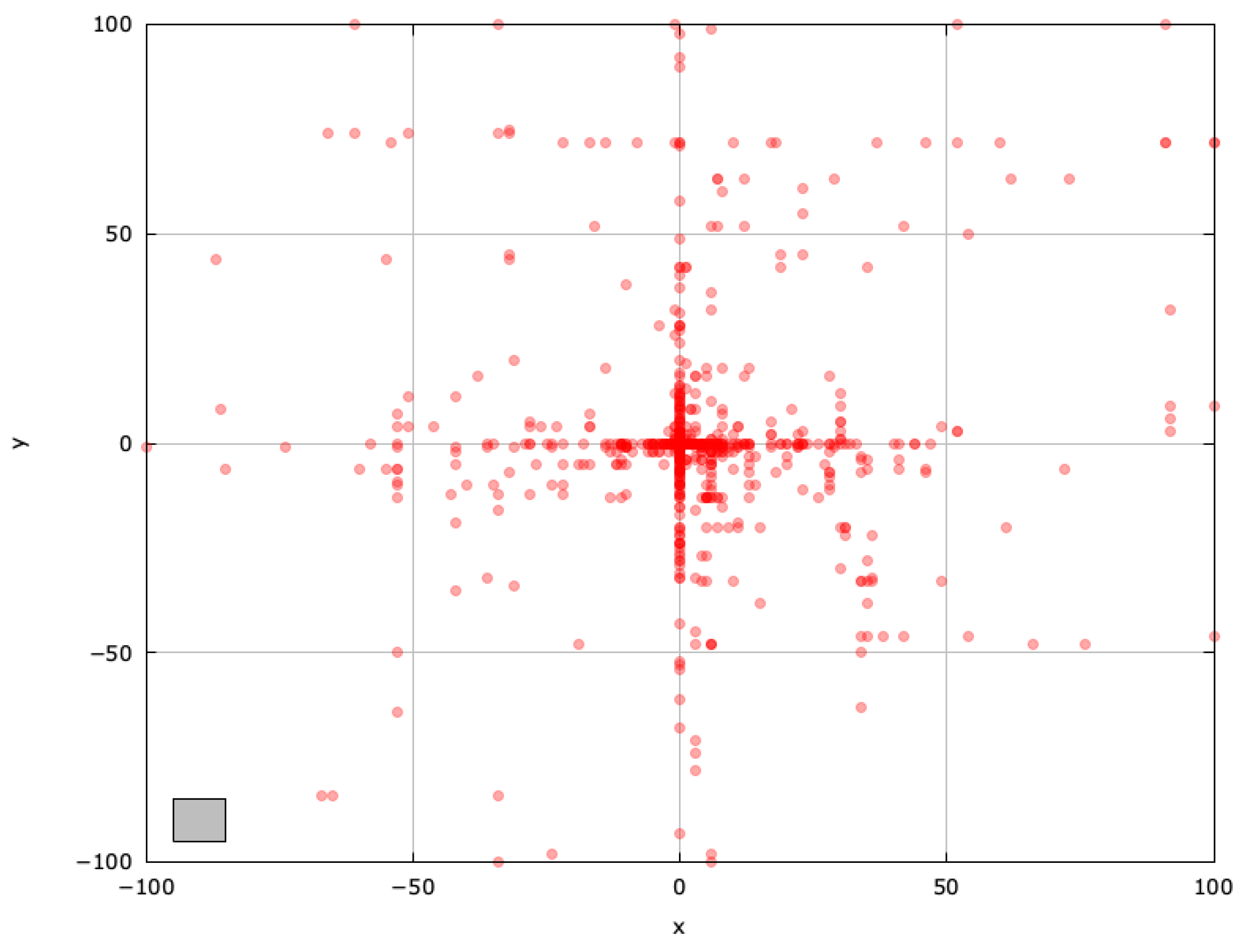
The ABC algorithm employs probability-based selection and a limit parameter to balance exploration and exploitation. Its search-space exploration shows vertical and horizontal patterns around influential solutions, attributable to scout bees sharing genotypic information probabilistically (Figure 4).
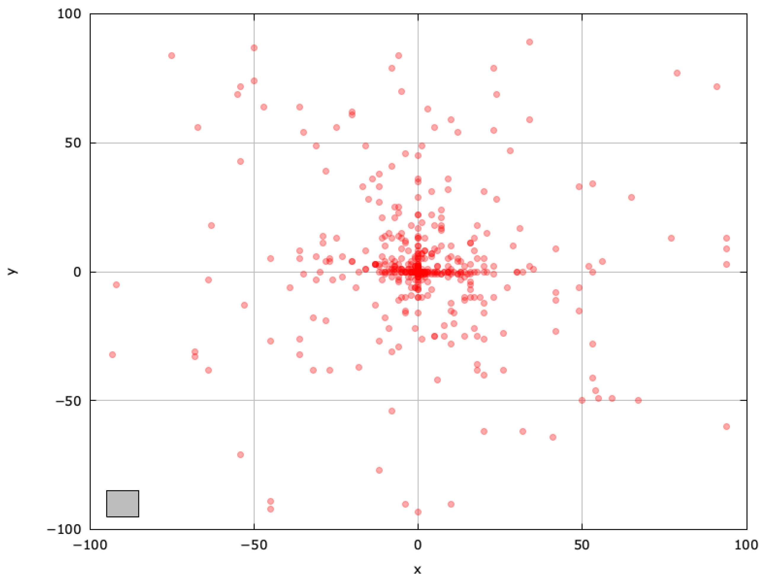
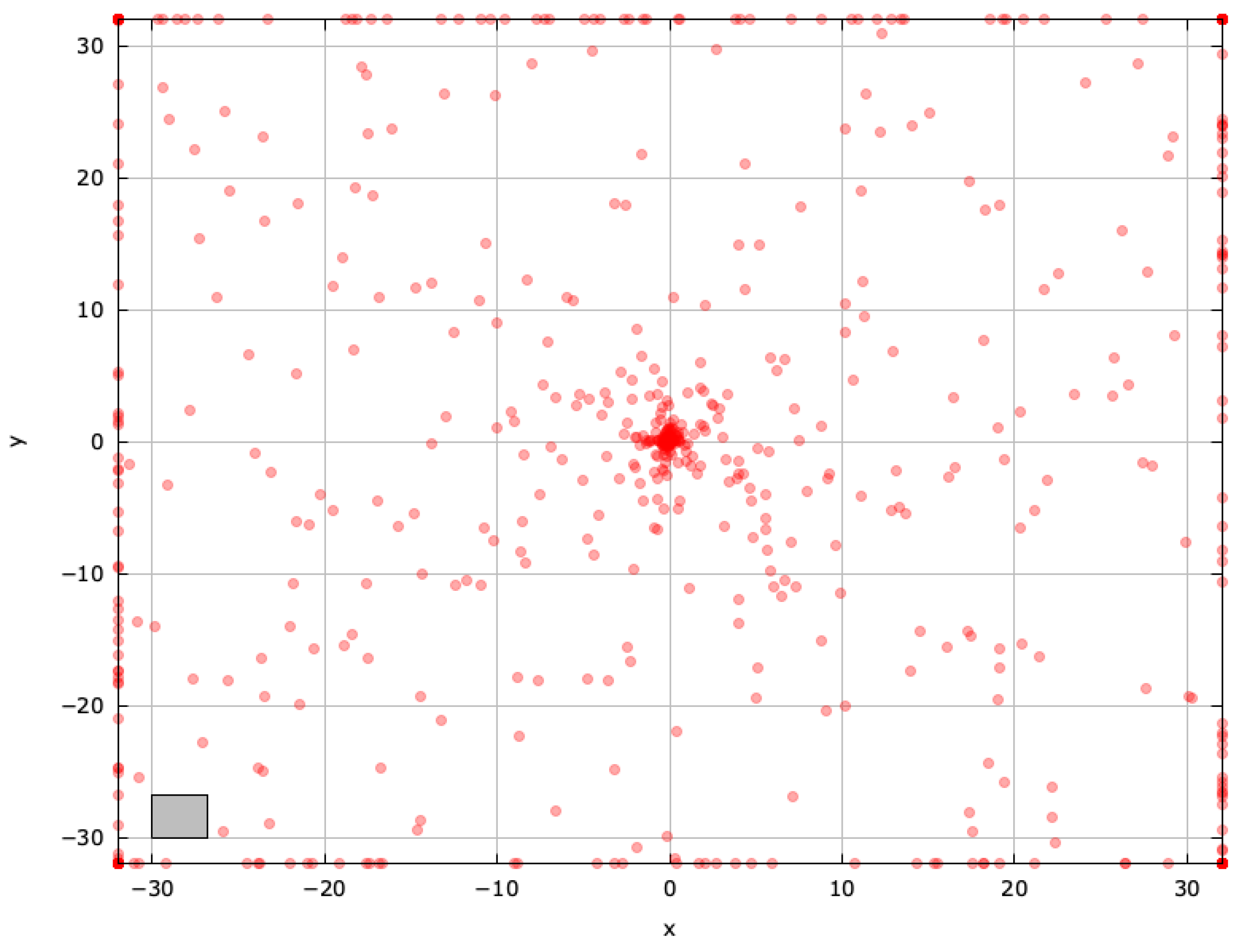
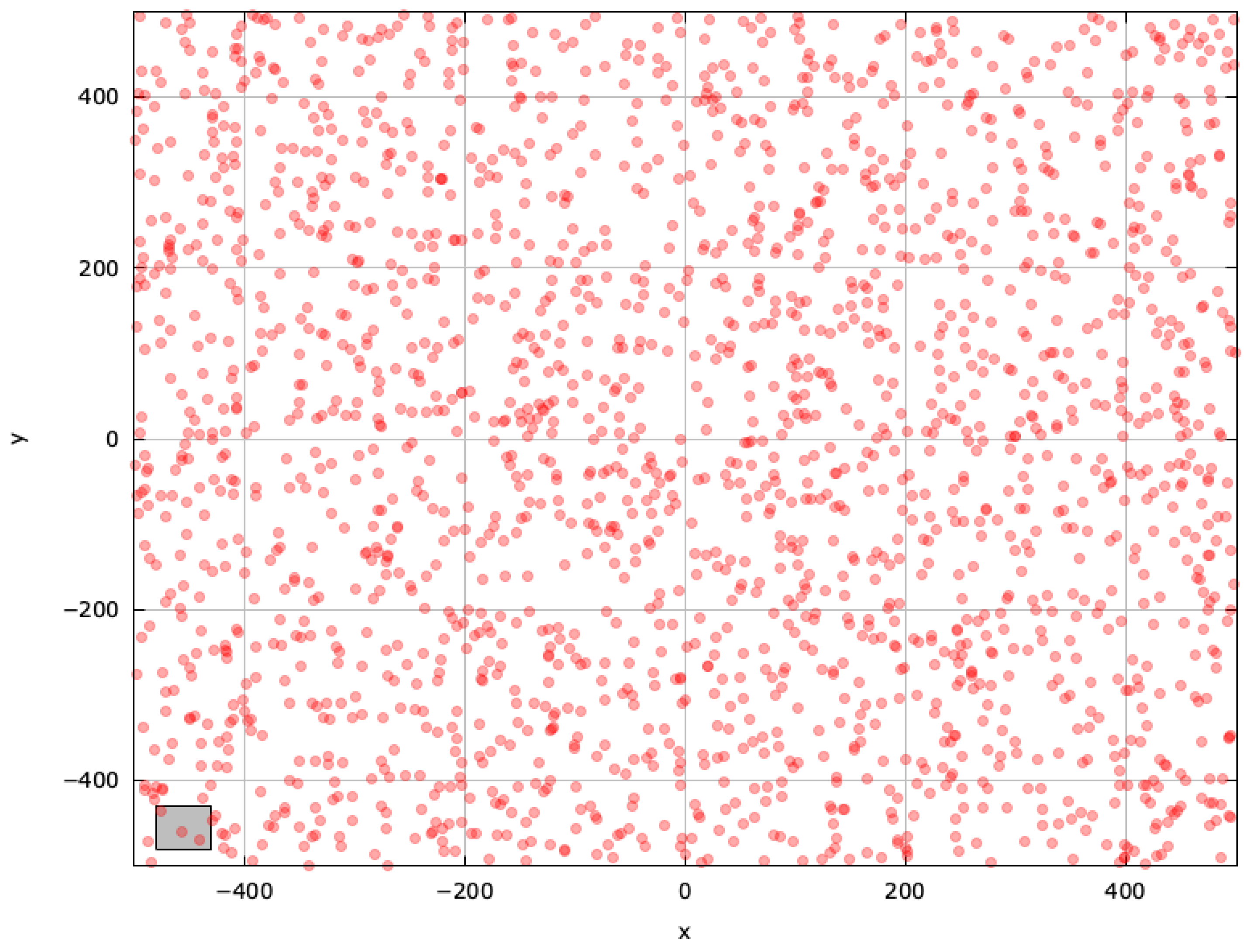
LSHADE’s success-history-based adaptation and population size reduction enable more diverse exploration, outperforming ABC (Figure 5).
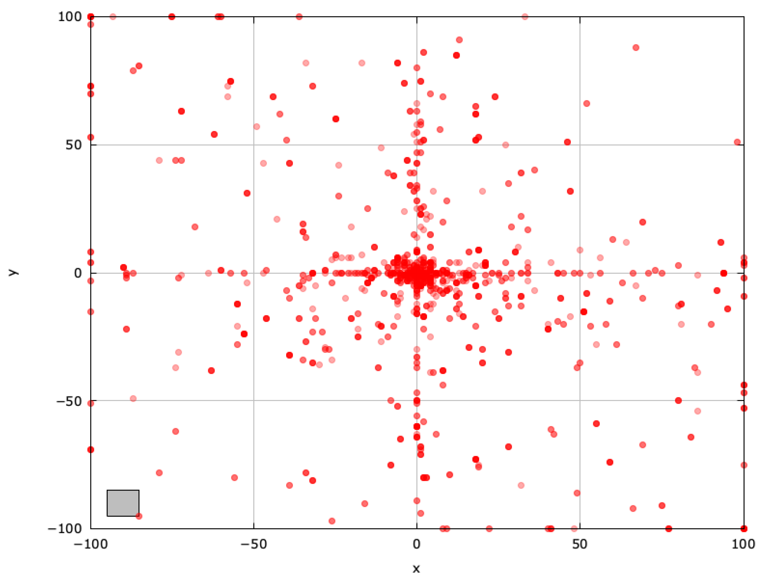
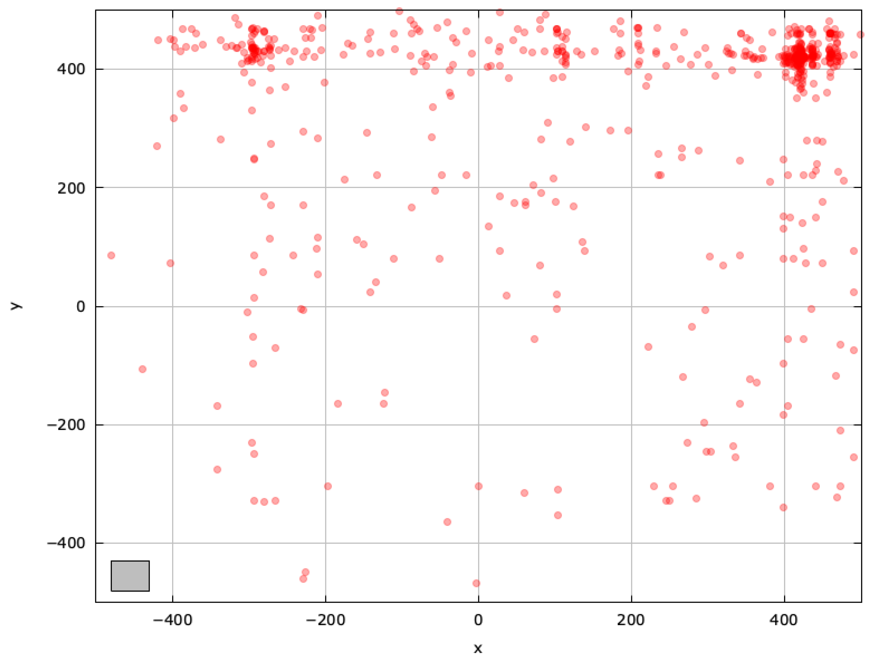
GAOA’s big, unpredictable movements enhance exploration, nearly locating the blind spot (Figure 6).
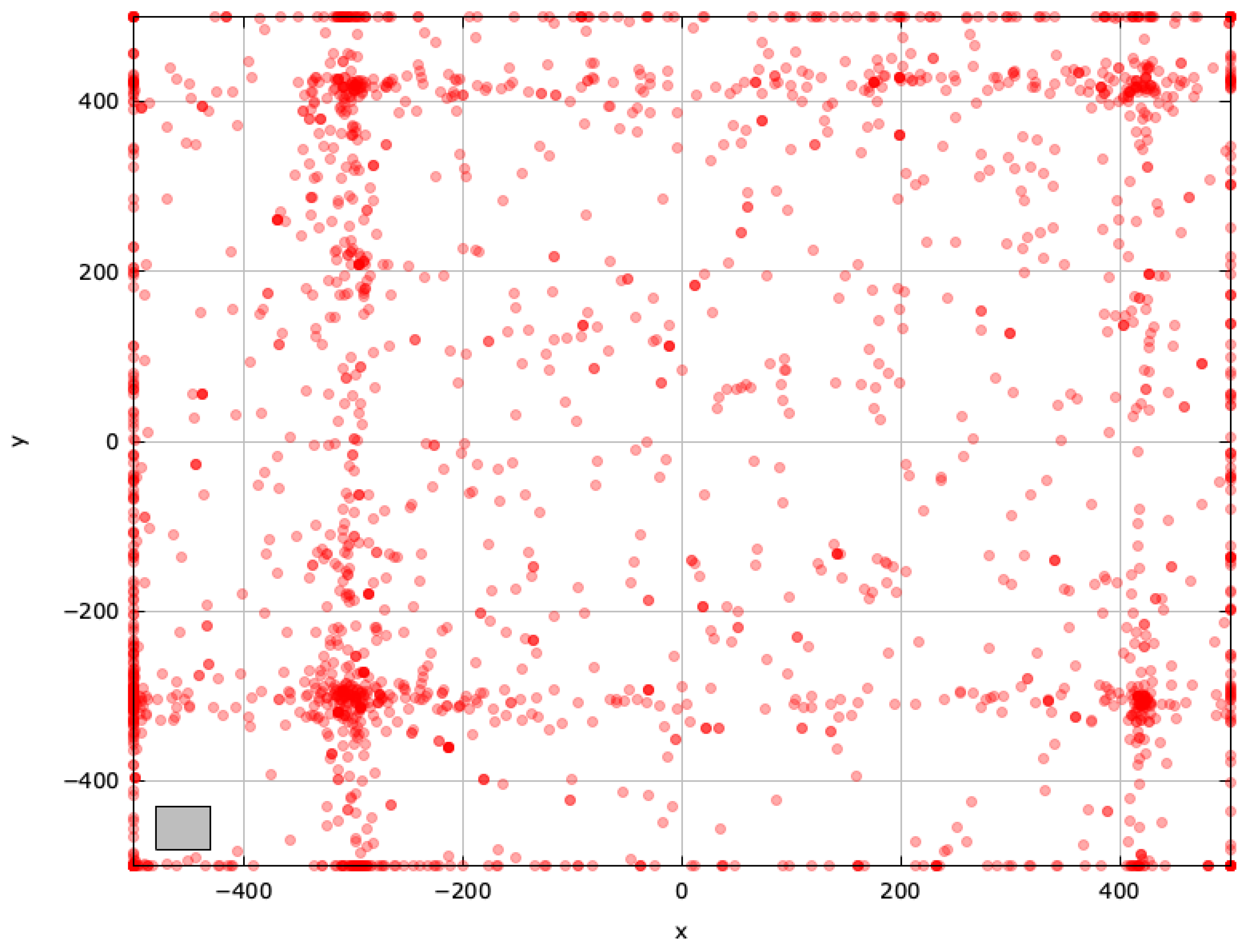
MRFO’s chain foraging promotes highly effective exploration with diverse solutions (Figure 7). Note that a good balance between exploration and exploitation is needed for an efficient search.
The self-adaptive jDElscop excels in exploration, but it can be hindered by intense pressure toward the local optima (Figure 8). A successful run, however, shows it searching around both optima thoroughly, highlighting strong exploitation (Figure 9).

LTMA Experiment Results for the SphereBS Problem

For each problem, we applied the original LTMA approach [10] with n [ 2 , 3 , 4 , 5 ] and memory precisions (Pr) of 3 and 6 (decimals in the solution space) and the stopping criterion M a x F E s . Since duplicates do not count as evaluations, we added a secondary stopping criterion, D A l l = 2 × M a x F E s , to prevent infinite loops. The results are averaged over 100 runs.
Table 1, Table 2 and Table 3 report the fitness evaluations used ( E V A L S P r ), total duplicates ( D A l l P r ), the fitness value ( F i t P r ), and the success rate ( S R ) for detecting blind spots. The best S R results for every n are formatted in bold. For n = 2 and n = 3 , RS outperformed the others on SphereBS (Table 1). Some algorithms underutilized the fitness evaluations (e.g., MRFO used 2086 of 8000 for n = 4 , or 26%, while generating 16,000 duplicates), suggesting premature convergence or success.

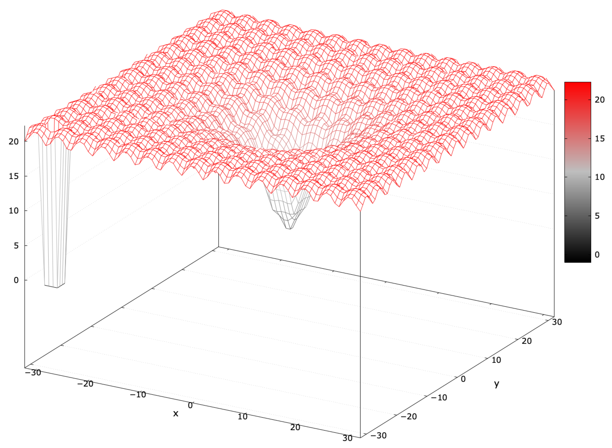
3.2. Ackley Blind Spot Problem (Medium)

The Ackley function features many local optima with small basins and a global optimum with a large basin [52]. MAs typically find the global optimum easily due to its gradual gradient. Adding a blind spot covering 0.05 % of the search interval (AckleyBS) increases the difficulty (Figure 10). The global optimum fitness is 1 .
Equation (2) defines the minimization problem:
f ( x ) = 20 exp 0.2 1 n i = 1 n x i 2 exp 1 n i = 1 n cos 2 π x i + 20 + e , if x i [ 32 , 32 ] for all i = 1 , , n and at least one x i [ 30 , 26.8 ] , 1 , if x i [ 30 , 26.8 ] for all i = 1 , , n .
where e is Euler’s number (≈2.7182818284).

LTMA Experiment Results for the AckleyBS Problem

Classified as medium difficulty, AckleyBS produced fewer duplicates than SphereBS, as confirmed by the results (Table 2). RS’s success rate in detecting blind spots remained consistent.
Figures presenting the search space exploration via MAs for the AckleyBS problem are provided in Appendix B.1.

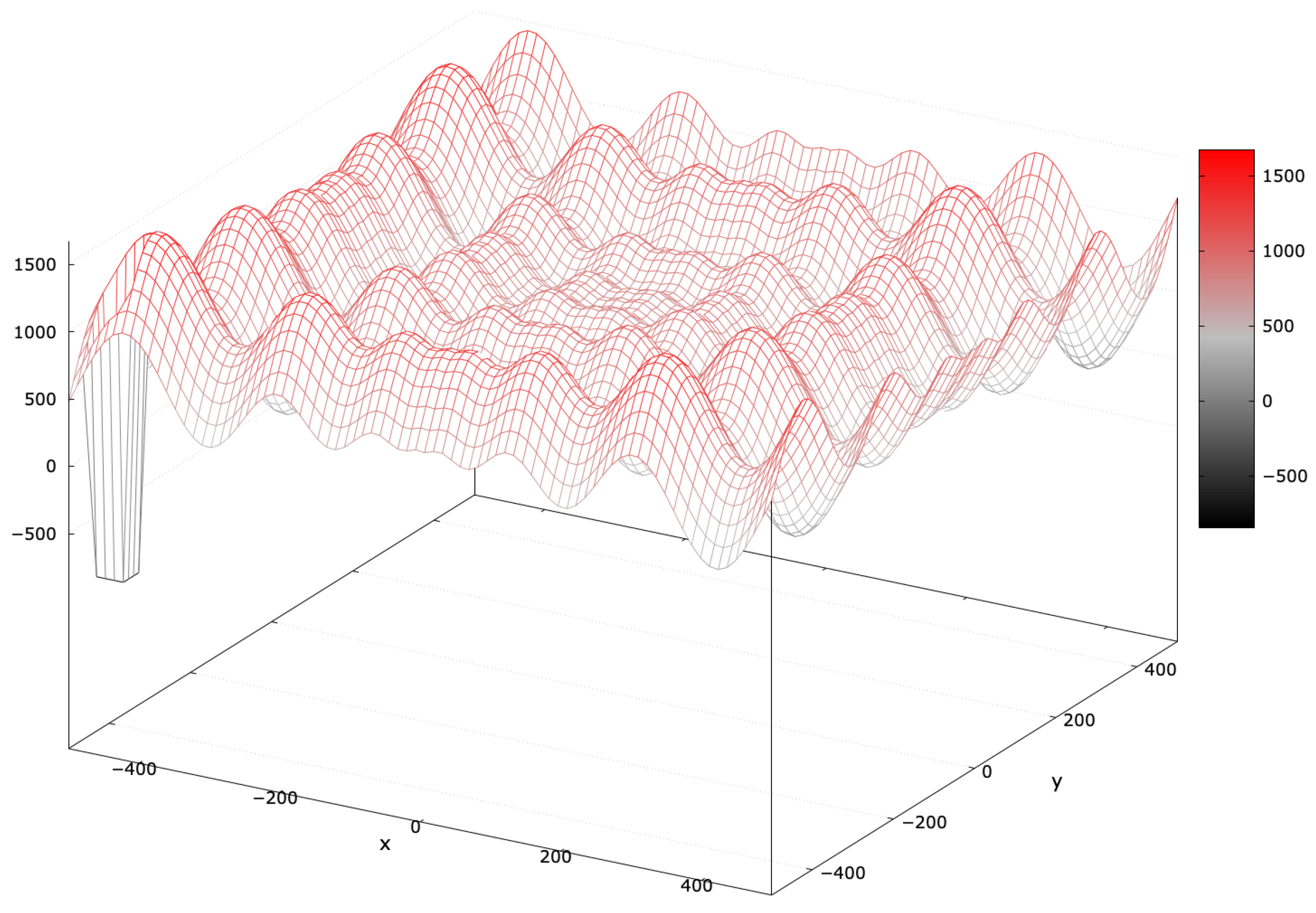
3.3. Schwefel 2.26 Blind Spot Problem (Hard)

The Schwefel 2.26 function includes a complex landscape with numerous local optima, and its global optimum is distant [53]. MAs often struggle due to its deceptive nature. Adding a blind spot covering 0.05 % of the search interval (SchwefelBS 2.26) heightens the challenge (Figure 11).
Equation (3) defines the minimization problem:
f ( x ) = i = 1 n x i sin | x i | , if x i [ 500 , 500 ] for all i = 1 , , n and at least one x i [ 480 , 430 ] , 418.9828872724337998079 · n 1 , if x i [ 480 , 430 ] for all i = 1 , , n .

LTMA Experiment Results for the SchwefelBS 2.26 Problem

The SchwefelBS 2.26 problem proved challenging, with RS achieving a 100% success rate for n = 2 and n = 3 (Table 3). Most MAs used all the fitness evaluations, except LSHADE, which used 2733 of 8000 for n = 4 with S R = 0 , indicating entrapment in the local optima.
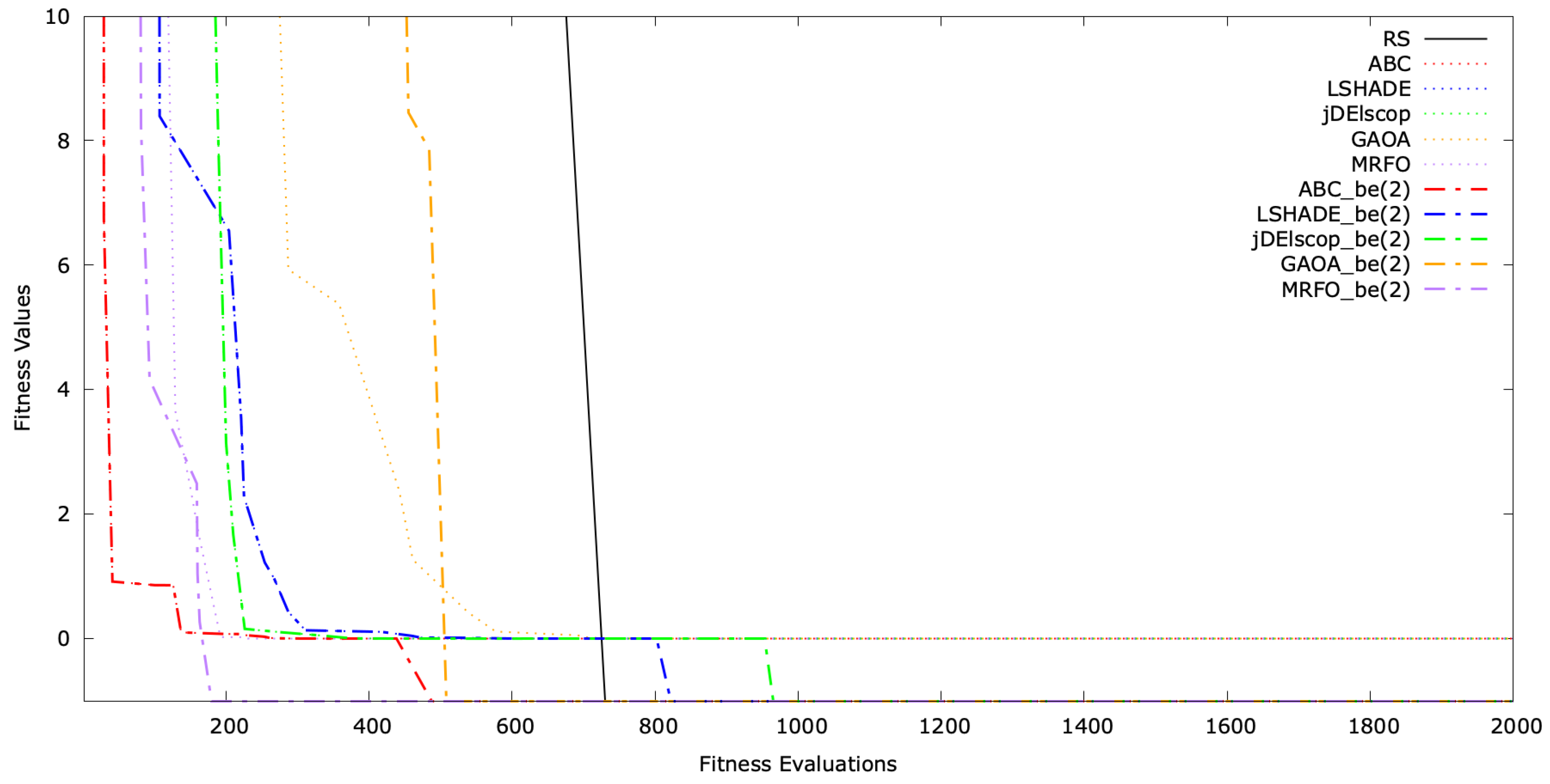
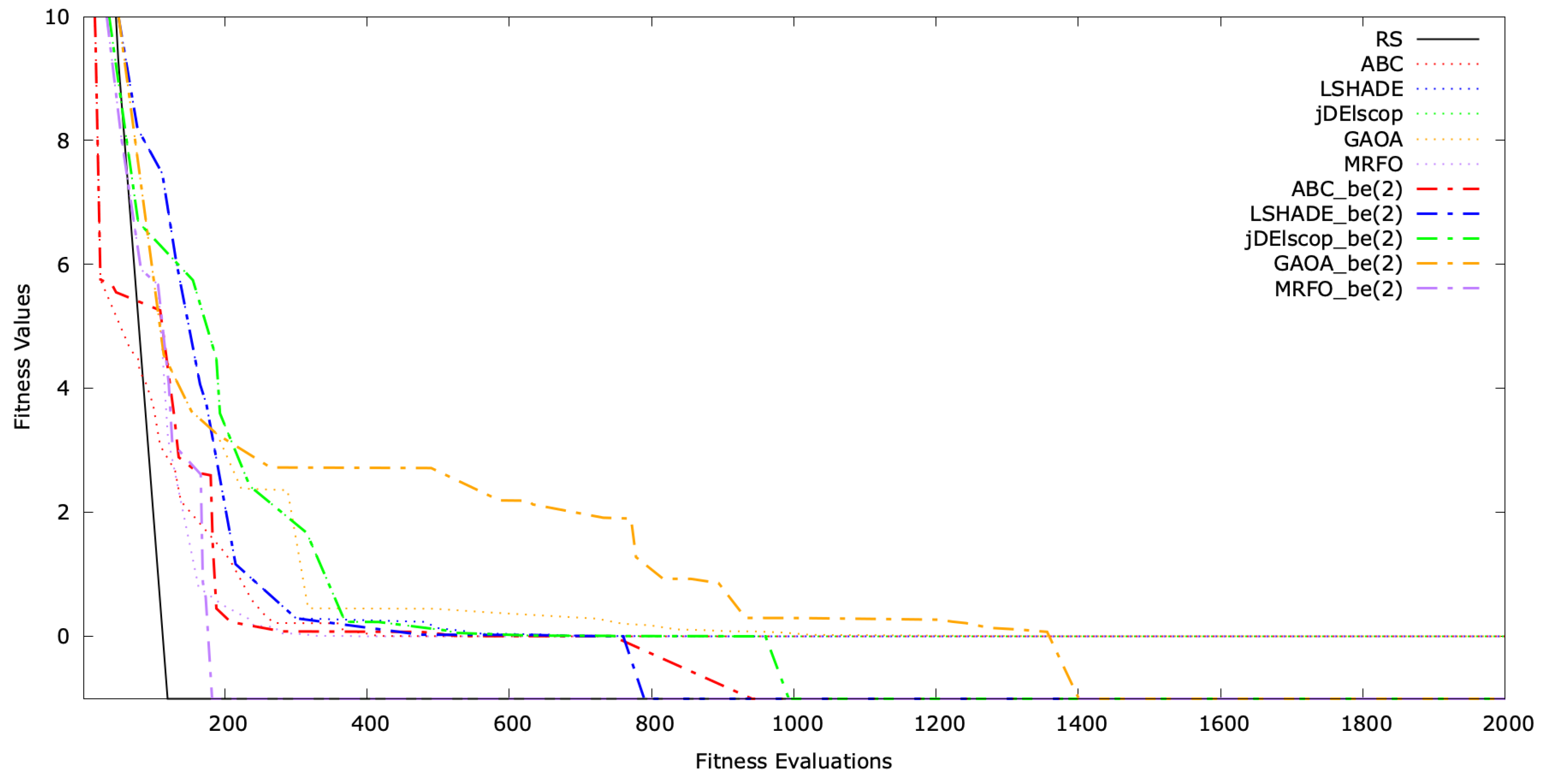
Figures presenting the search space exploration with MAs for the SchwefelBS 2.26 problem are provided in Appendix B.2. A further convergence analysis of the selected MAs’ runs with benchmark problems is detailed in Appendix C.

3.4. Blind Spot Problem Benchmark

We created a benchmark including SphereBS, AckleyBS, and SchwefelBS 2.26 for n [ 2 , 3 , 4 , 5 ] , totaling 12 problems with M a x F E s set to 2000, 6000, 8000, and 10,000. For LTMA, the precision was set to 3.
For statistical analysis, we employed the EARS framework with the Chess Rating System for Evolutionary Algorithms (CRS4EAs), based on the Glicko-2 system [54,55]. CRS4EAs assigns ratings via pairwise comparisons (win, draw, or loss), defining a draw when the fitness values differ by less than 0.001, mitigating bias from the averaging fitness values affected by blind spots. Each MA, initially assigned a rating of 1500 and a rating deviation of 250, undergoes 30 independent optimization runs per benchmark problem in a tournament [43]. Pairwise comparisons, based on fitness values, update ratings using the Glicko-2 system, with the process repeated across 30 tournaments to assess performance robustness [
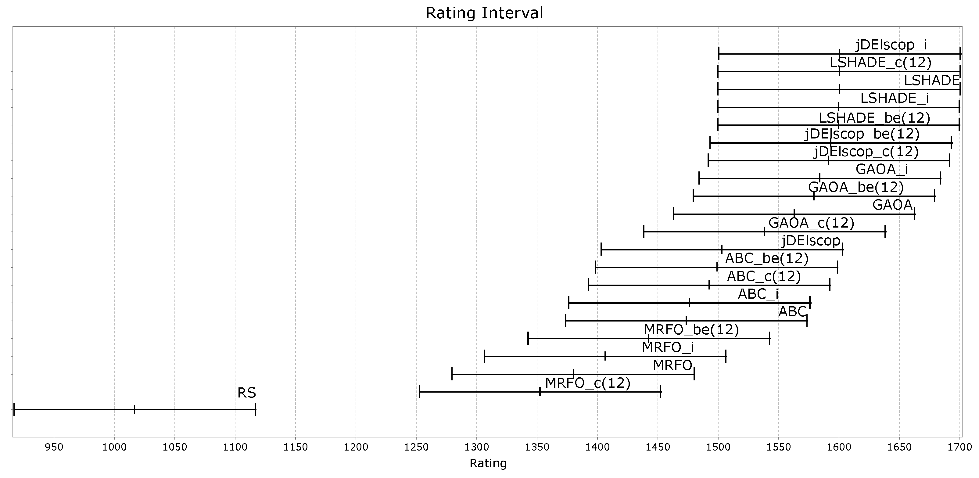
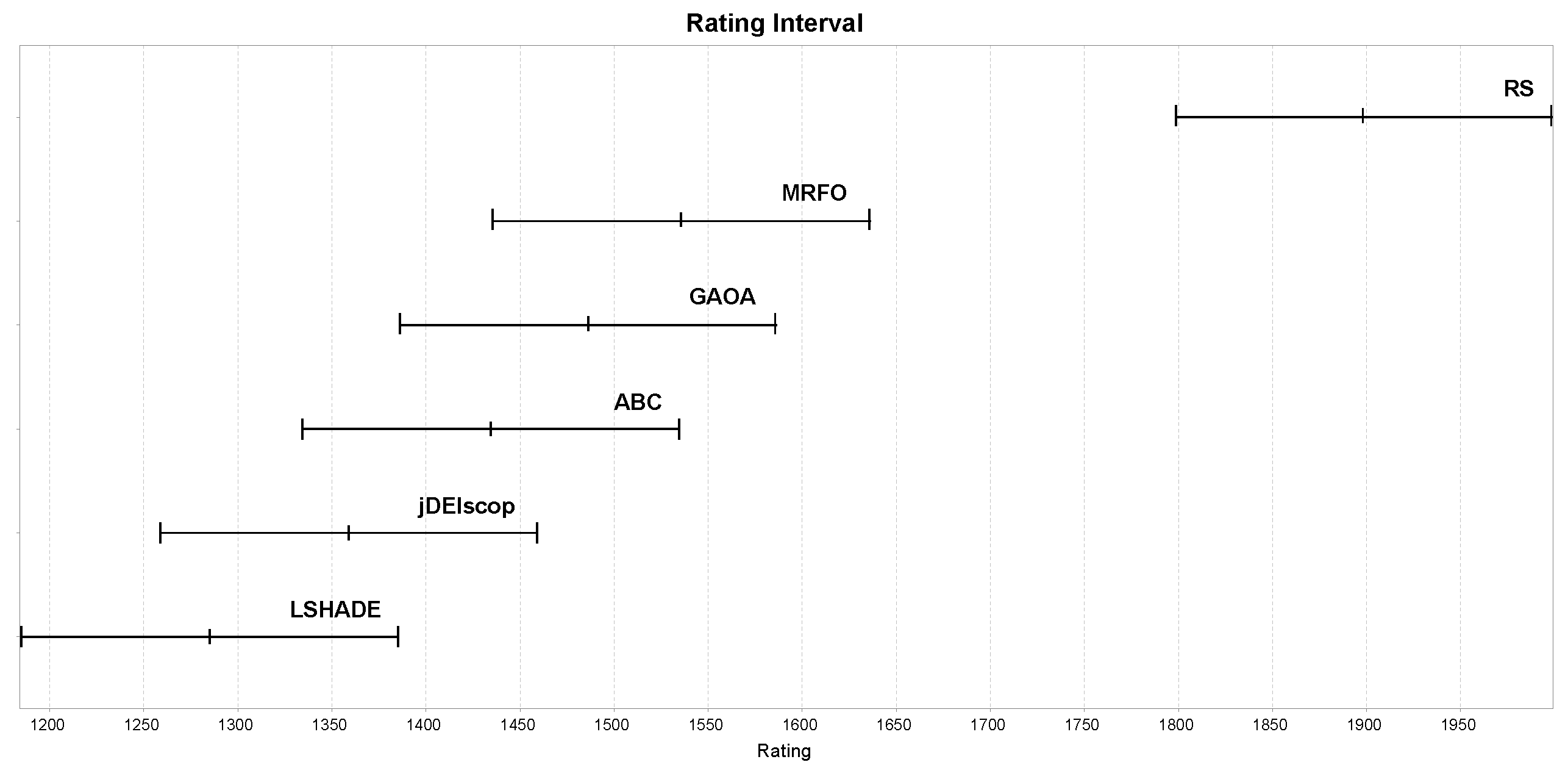
10]. For the calculated ratings and confidence intervals, overlapping intervals indicate no significant difference. For n = 2 , RS outperformed MAs statistically significantly in detecting blind spots, as shown in Figure 12, suggesting limitations in MAs’ exploration of complex landscapes. The RS excelled at detecting blind spots (Figure 12), raising concerns about MAs.
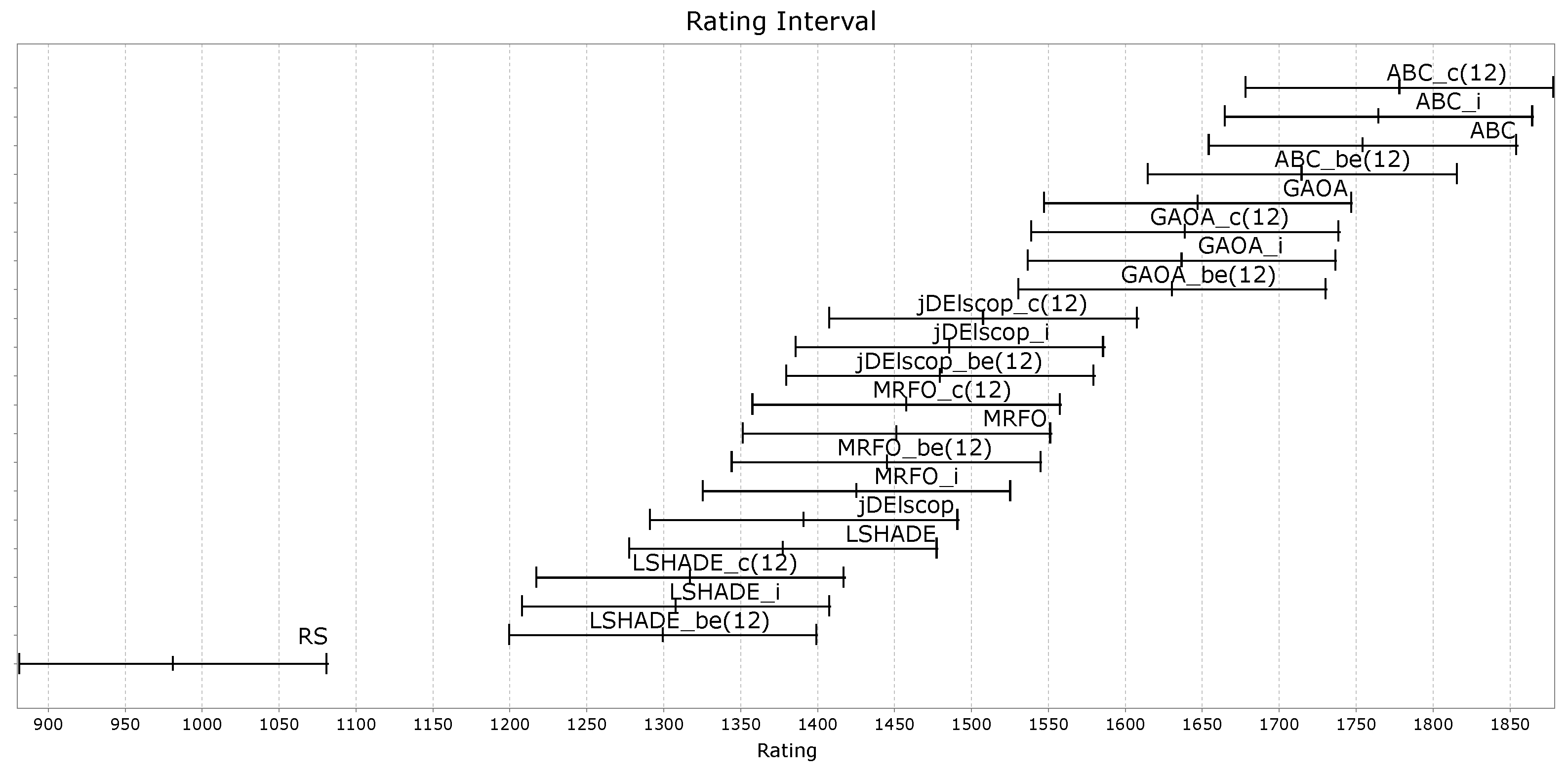
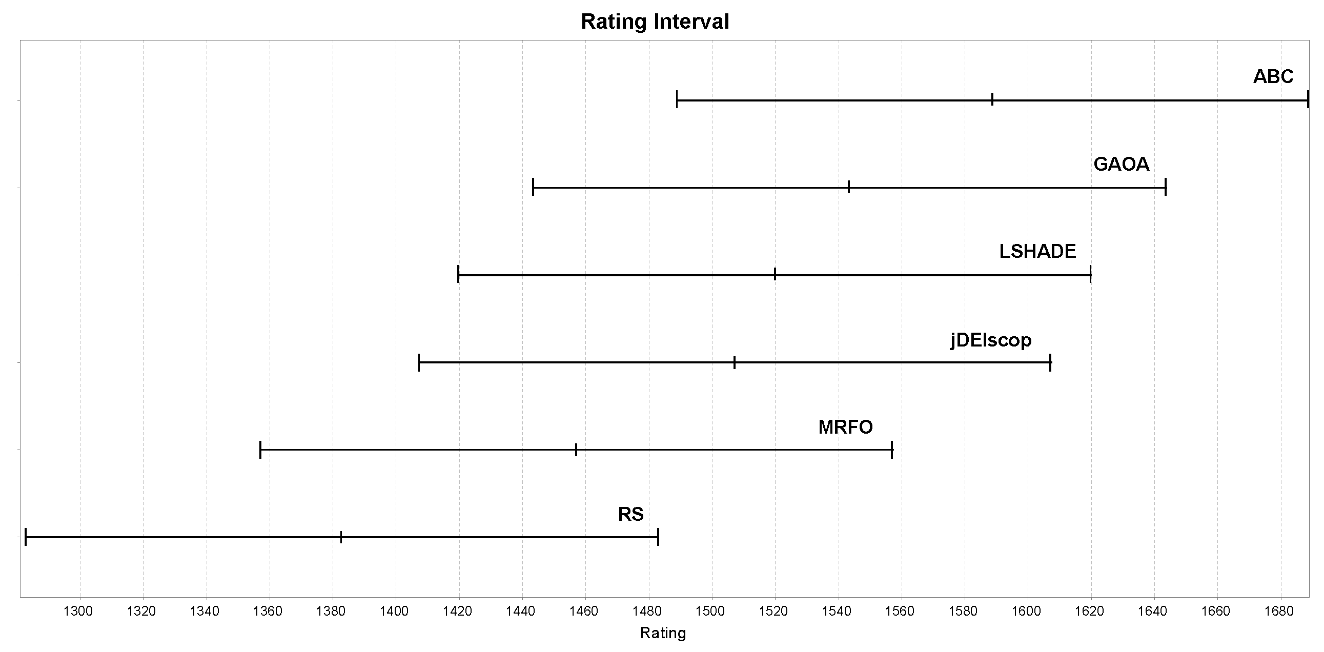
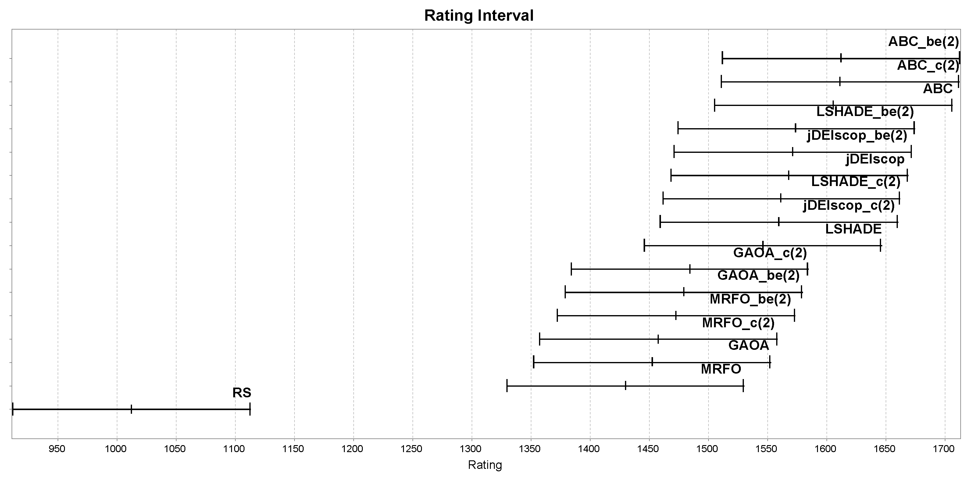
Benchmark results with blind spots revealed that only the ABC algorithm outperformed the RS baseline statistically significantly in terms of ratings, as shown in Figure 13, indicating that the selected MAs struggled to explore complex landscapes effectively [
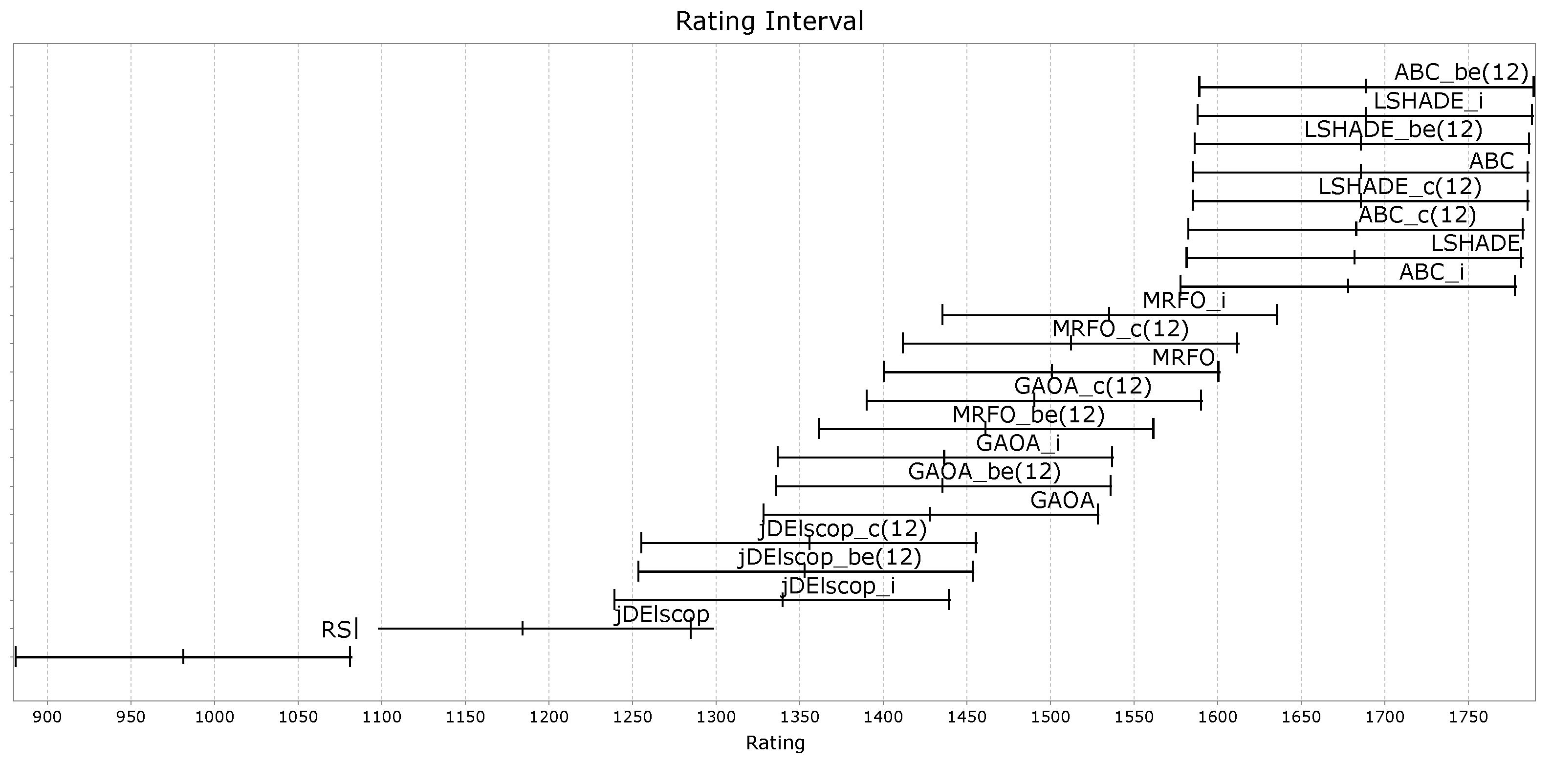
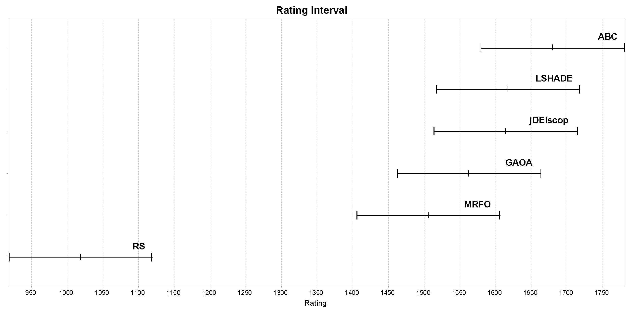
43]. To provide context, we repeated the experiments with identical settings on standard benchmark problems without blind spots. These results confirmed the expected superiority of MAs, with higher ratings across all the algorithms, as illustrated in Figure 14 [10].

4. LTMA+

LTMA+ is a novel approach based on LTMA [10] that enhances the exploration mechanics of MAs by leveraging duplicate detection. This mechanism operates independently of the MAs, ensuring a fair algorithm comparison. LTMA+ functions as a meta-operator applicable to any metaheuristic, improving success rates without altering the algorithms themselves.
LTMA [10] is extended with a duplicate replacement strategy: when a duplicate solution is detected, the solution, x, is replaced with a newly generated solution, x , (Figure 15). This approach aims to avoid local optima and enhance search-space exploration. However, it raises concerns about its impact on the core mechanics of optimization algorithms, as it may alter exploration procedures and disrupt the exploitation phase significantly. We conducted a detailed analysis in which duplicate solutions were created to address these concerns (Appendix E).
The frequency of duplicates, D A l l , is observable in Table 1, Table 2 and Table 3. The percentage of duplicates varies by problem, dimension, population size, and algorithm. However, these data alone do not reveal how often a solution is duplicated or the frequency of such duplicates (LTMA access hits). For instance, if a solution, x 1 , is duplicated 1000 times ( H i t ( x i ) = 1000 ), it might indicate a local optimum trap. The key distinction is whether a single solution generates many duplicates or multiple solutions are duplicated. This information can be used to trigger a forced exploration of new search-space regions.
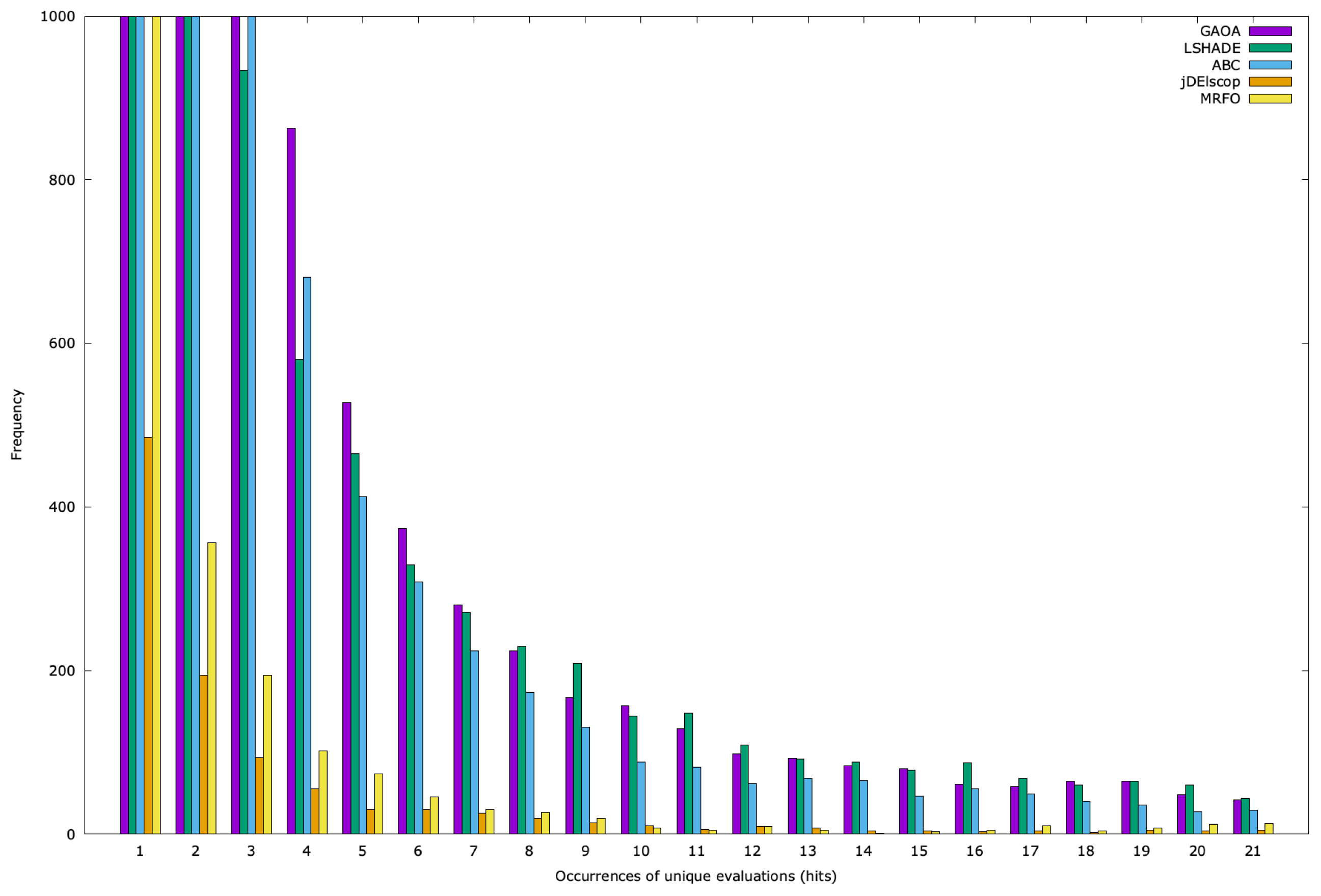
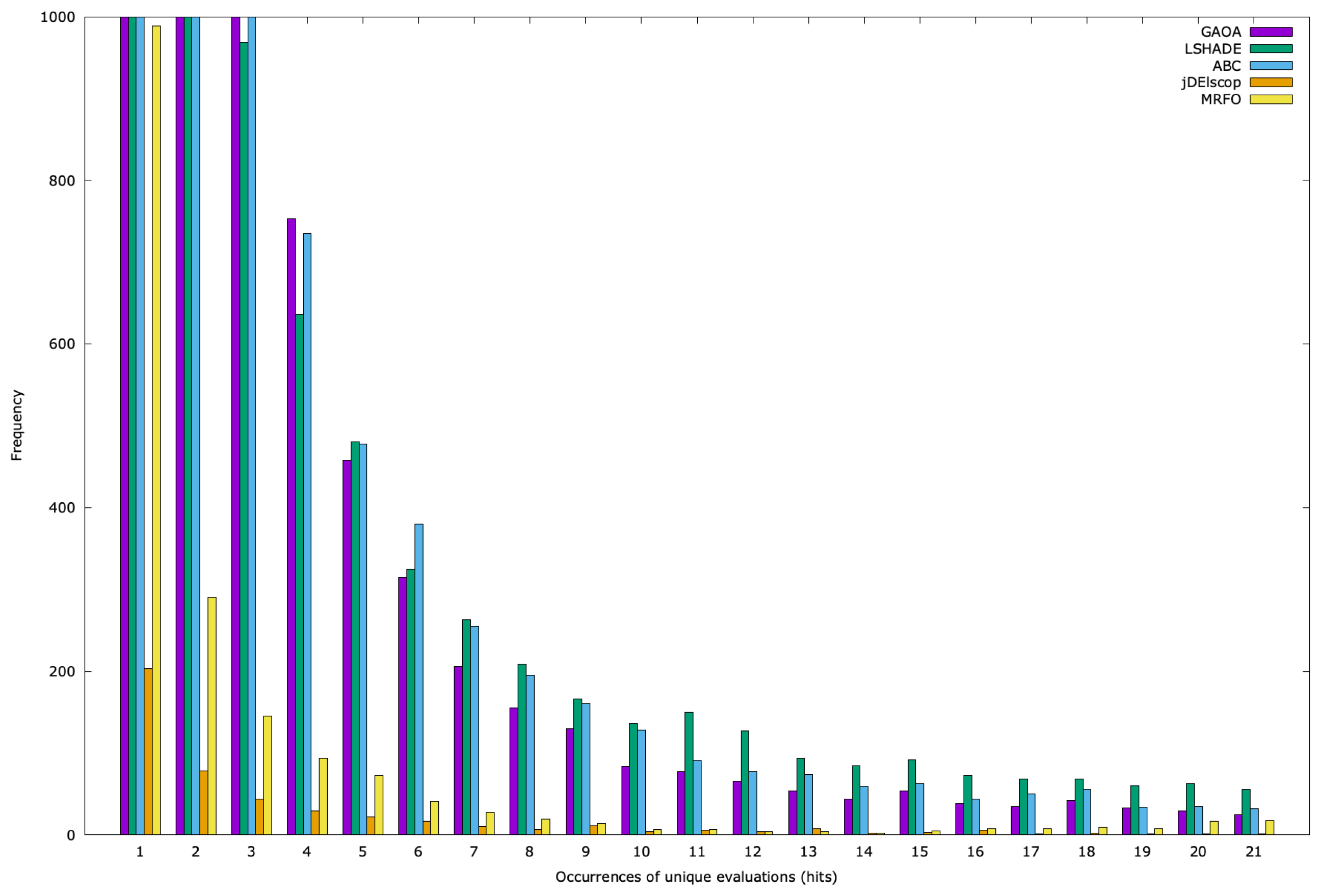
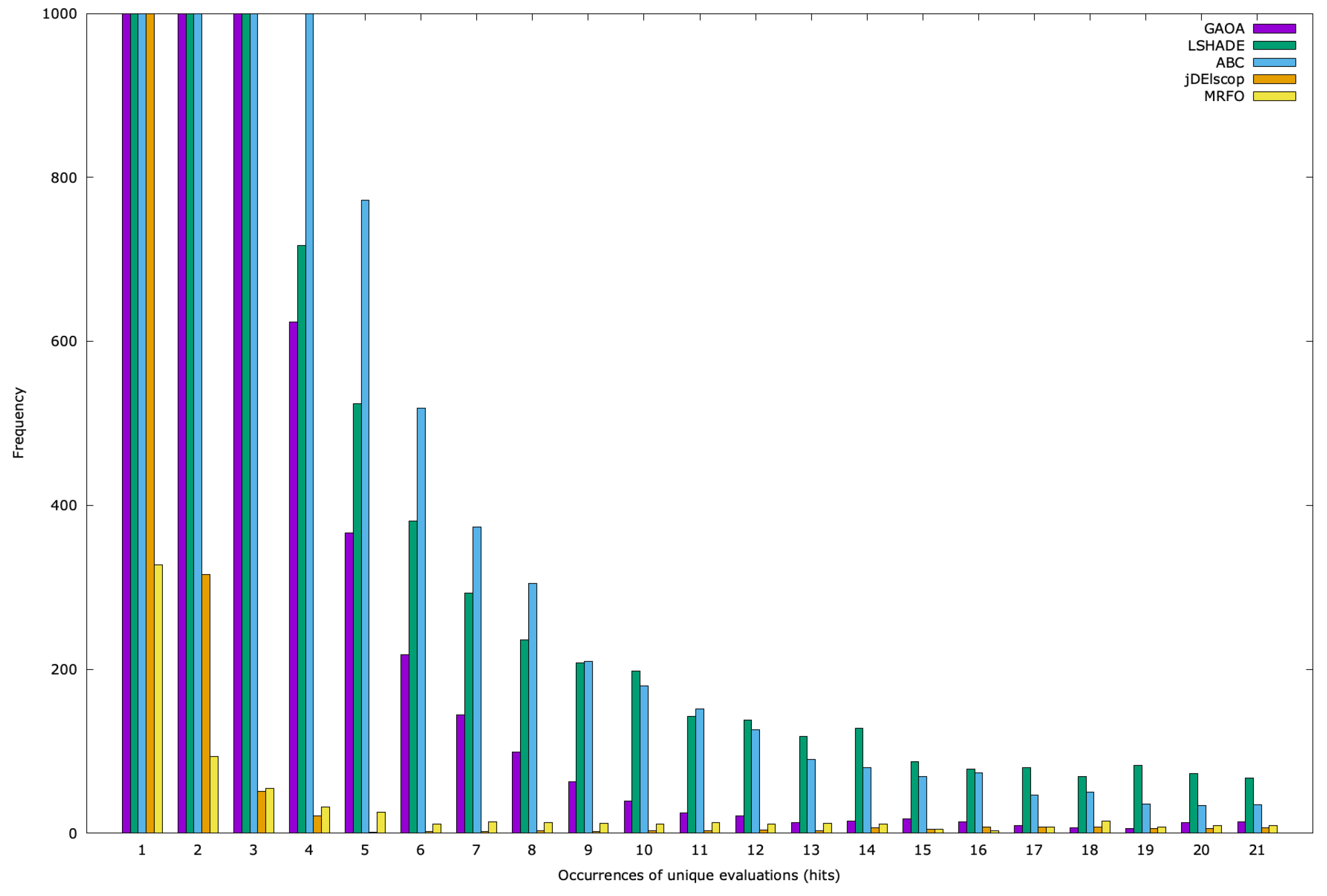
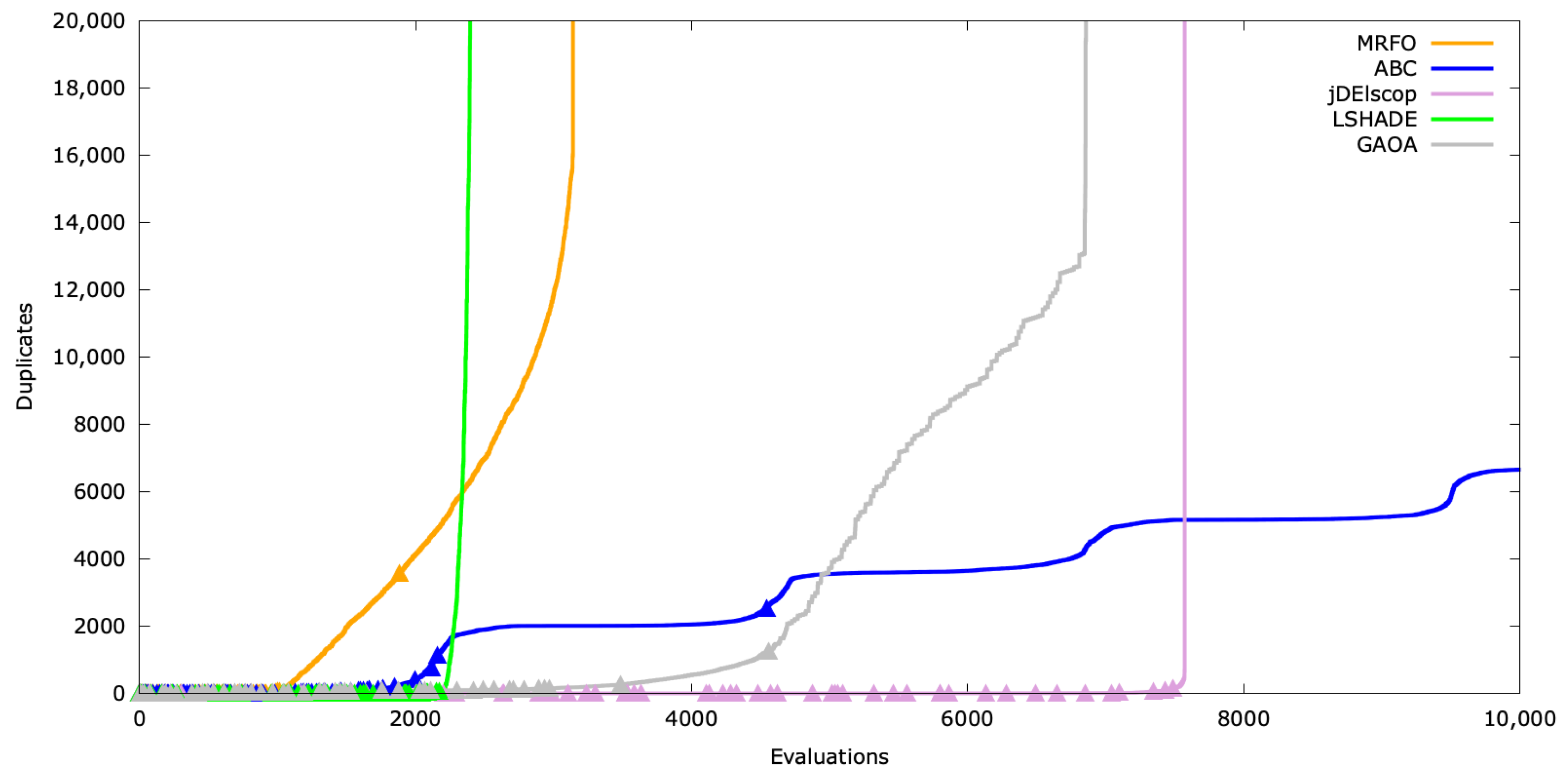
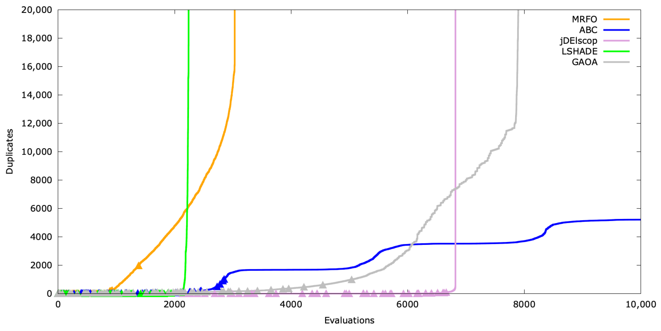
A detailed analysis of the LTMA access hits showed that most solutions had low hit counts, while a few had high ones (Figure A19, Figure A20 and 
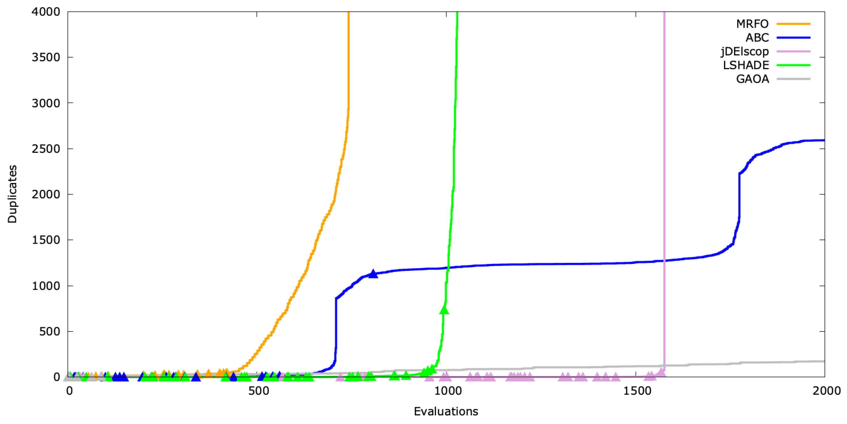
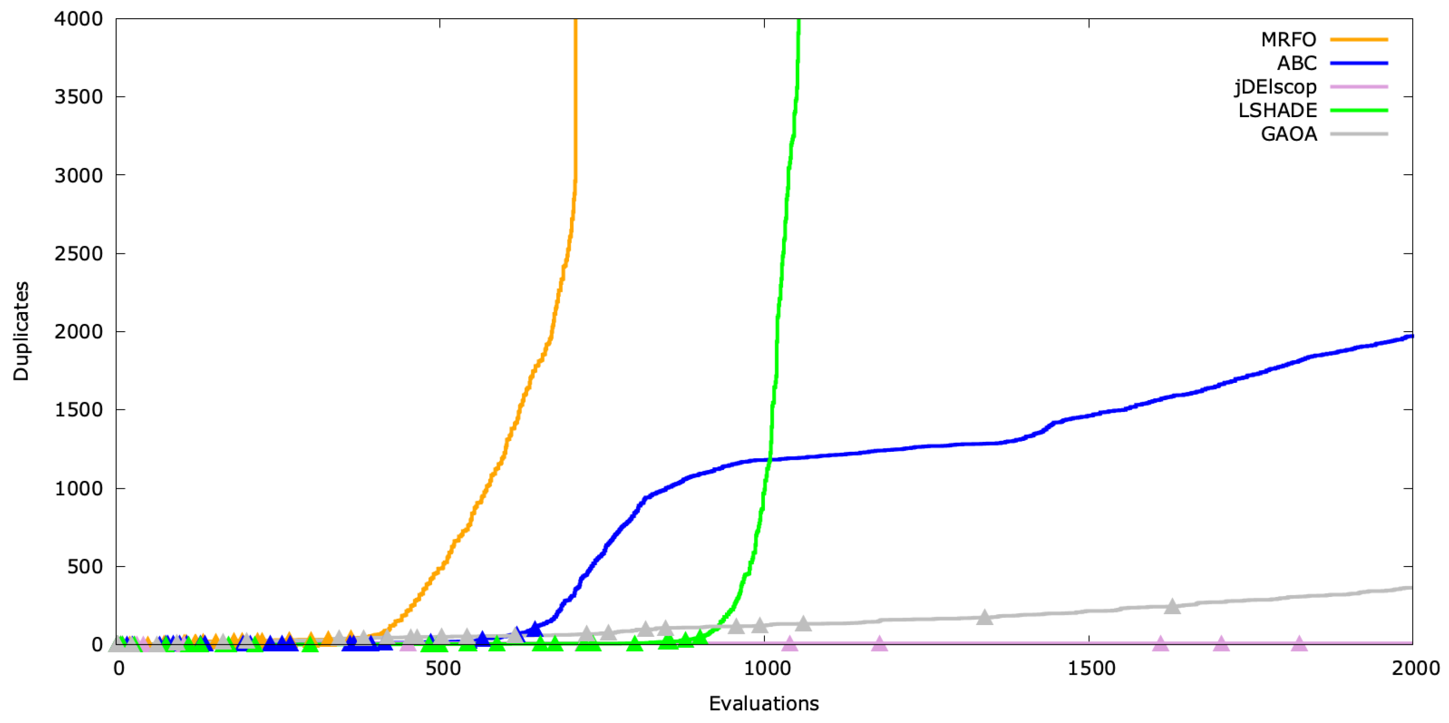
Figure A21). This suggests effective search-space exploration. However, the graph’s tail (rare high-hit individuals) indicates a few solutions with very high hit counts, where the total sum of hits is concentrated, potentially signaling entrapment in the local optima. To clarify this, we generated a running sum of hits graph for duplicate creation (Appendix D). The analysis of duplicate creation timing is also crucial for understanding the behavior of LTMA+ and its impact on optimization algorithms. By examining the timing of duplicate creation, we can identify when the algorithm is likely to become trapped in local optima (Appendix E).
Our analysis identified two key parameters to guide the exploration:
  • Number of hits (Hit): if a solution is generated x times, a new, non-revised solution replaces it.
  • Timing of duplicates: new solutions are created after x sum of memory hits ( D A l l ).
These parameters defined the LTMA+ strategies that preserve MAs’ internal exploration and exploitation dynamics, avoiding premature convergence.

4.1. Generating New Candidate Solutions

Mimicking RS, we could generate random solutions for additional exploration, but this would ignore the prior search information. From Figure 4, Figure 5, Figure 6, Figure 7 and Figure 8, we observed that blind spots near the current solutions are more likely to be found during exploitation. Thus, we propose generating solutions using three random generation variants: basic random, random farther from the duplicate, and random farther from the current best.
We use a triangular probability distribution to generate a solution randomly, likely far from a selected position (Appendix F). For each dimension x i , we generate a random position from the current position to the search space boundary, deciding to move left or right randomly:
x i = x i + upperLimit i x i · triangularRandom ( 0 , 0.9 , 1 ) , if random ( 0 , 1 ) < 0.5 , x i lowerLimit i x i · triangularRandom ( 0 , 0.9 , 1 ) , otherwise ,
where upperLimit i and lowerLimit i are search-space bounds, and triangularRandom ( a , c , b ) generates a number with a = 0 , b = 1 , and mode c = 0.9 .

4.2. Strategies

Using exploration triggers and random generation methods, we define the following strategies:
  • Ignore duplicates (i): ignores duplicates, simulating LTMA.
  • Random (r): generates a basic random solution for duplicates, simulating RS.
  • Random from current (c): generates a random solution farther from the duplicate.
  • Random from best (b): generates a random solution farther from the current best solution.
  • Random from best extended (be): generates random solutions farther from the current best for the next 100 evaluations.
Strategies may include a H i t parameter, replacing duplicates only after a specified hit count, or a parameter for the number of prior duplicate evaluations to initiate replacement.

5. Experiments

Having defined various LTMA+ strategies, we now evaluate them empirically through experiments. We compared LTMA+ strategies with the original LTMA and MAs from Section 2 on the Blind Spot benchmark from Section 3.4.
In our experiments, we reported the success rate ( S R P ) and fitness value ( F i t P ) for LTMA+ with precision Pr = 3, averaged over 100 runs. We also analyzed the influence of the Hit parameter as a trigger, testing values 1, 2, and 5. We include results for basic LTMA and RS for comparison.

5.1. L T M A + r

The r strategy generates a random individual when the LTMA+ duplicate hit trigger (Hit) is reached, tested for H i t = 1 , 2 , 5 ( L T M A + r ( 1 ) , L T M A + r ( 2 ) , L T M A + r ( 5 ) ). The results show a significantly higher number of discovered blind spots with the r strategy (Table 4). The success rates for H i t = 1 and H i t = 2 were similar, but they were lower for H i t = 5 . Notably, GAOA for n = 4 and n = 5 performed better without LTMA+ ( S R = 20 ), an issue addressed in the next section.
Similar results were observed for SphereBS and SchwefelBS 2.26 (Table A1 and Table A2).

5.2. L T M A + c

The c strategy generates a random individual farther from the current one when the Hit trigger is reached, tested for H i t = 1 , 2 , 5 ( L T M A + c ( 1 ) , L T M A + c ( 2 ) , L T M A + c ( 5 ) ). We expected c to outperform r due to its generation of solutions farther from the current one. The results in Table 5 confirm this, with the best performance at H i t = 1 .
Similar outcomes were seen for SphereBS and SchwefelBS 2.26 (Table A3 and Table A4).

5.3. L T M A + b

The b strategy generates a random individual farther from the current best solution when the Hit trigger is reached, tested for H i t = 1 , 2 , 5 ( L T M A + b ( 1 ) , L T M A + b ( 2 ) , L T M A + b ( 5 ) ). Since duplicates often cluster around the current best, we that anticipated b would perform similarly to c. Table 6 confirms this expectation.
Comparable results were obtained for SphereBS and SchwefelBS 2.26 (Table A5 and Table A6).

5.4. L T M A + b e

The b e strategy includes an e x t e n d parameter, defining how many evaluations generate random individuals from the best solution after the Hit trigger. With e x t e n d = 1 , it mirrors b. We set e x t e n d to 0.1% of M a x F E s (e.g., 8 for M a x F E s = 8000 ), generating random individuals for the next eight evaluations. The results are presented in Table 7.
No significant success rate improvement was observed, though we expect b e to be more effective in runs with fewer duplicates. We suggest lower e x t e n d values.
Similar results were seen for SphereBS and SchwefelBS 2.26 (Table A7 and Table A8).

5.5. Evaluating of LTMA+ Strategies on the Blind Spot Benchmark

Similar experiments to those described in Section 3.4 were conducted, but with selected MAs wrapped with various LTMA+ strategies to enhance the exploration of blind spots in benchmark problems. We compared standard MAs against those wrapped with LTMA+ strategies, such as L T M A + b e ( 2 ) ( H i t = 2 ), on the Blind Spot benchmark problems, with the Glicko-2 rating results presented in Figure 16. The MAs wrapped with LTMA+ strategies outperformed the MAs on the Blind Spot benchmark problems statistically significantly, with L T M A + b e ( 2 ) , employing solution-based randomization from the best solution, achieving the highest Glicko-2 ratings, followed by L T M A + c ( 2 ) , as shown in Figure 16.
Injecting random individuals helps escape the local optima, but it may degrade performance on problems without blind spots. Testing on a no-blind-spot benchmark (Figure 17) showed that LTMA+ strategies still outperformed baselines, with no significant difference between the problem types.

5.6. Evaluation of LTMA+ Strategies on Benchmarks Without Blind Spots

With the modifications introduced in LTMA+, it is essential to evaluate their impact compared to the original LTMA approach on problems without blind spots. Since these strategies primarily manage generated duplicates, we expect minimal performance differences between LTMA+ and LTMA on such problems. However, replacing duplicates with randomly generated individuals might disrupt the exploitation phase, potentially leading to solutions with reduced precision.
For a thorough comparison with the original LTMA method, we selected two test cases from the original LTMA paper: the CEC’15 benchmark problem (Experiment 2) and the real-world soil problem (Experiment 3) [10]. We set the Hit parameter to 12, using benchmark problems with n = 10 and MaxFEs = 10,000.
As anticipated, the results for the CEC’15 benchmark problem revealed no significant performance differences between LTMA+ and LTMA. For LSHADE, ABC, and MRFO, LTMA+ outperformed the original LTMA slightly (Figure A29). For the soil problem, we optimized three instances (TE1, TE2, and TE3), yielding similar outcomes with no notable differences between LTMA+ and LTMA (Figure A32). Interestingly, the rating rankings varied by instance: jDElscop excelled in TE1, while ABC led in TE2 and TE3 (Figure A30, Figure A31 and Figure A32).
More information on the experiments is available in Appendix G.5.

6. Discussion

The proposed LTMA+ approach offers advantages, disadvantages, and considerations. To begin the discussion, we first highlight its positive aspects.

6.1. The Good

LTMA+ enhances the robustness of MAs by facilitating a transition from duplicate creation to exploration, often preventing algorithm stagnation. This is particularly effective when the total number of evaluations is unknown. Even RS can outperform MAs when an algorithm is trapped in a local optimum. By leveraging prior evaluations, such as the current duplicate or best solution, LTMA+ generates smarter random individuals positioned farther from the current search space, promoting exploration.
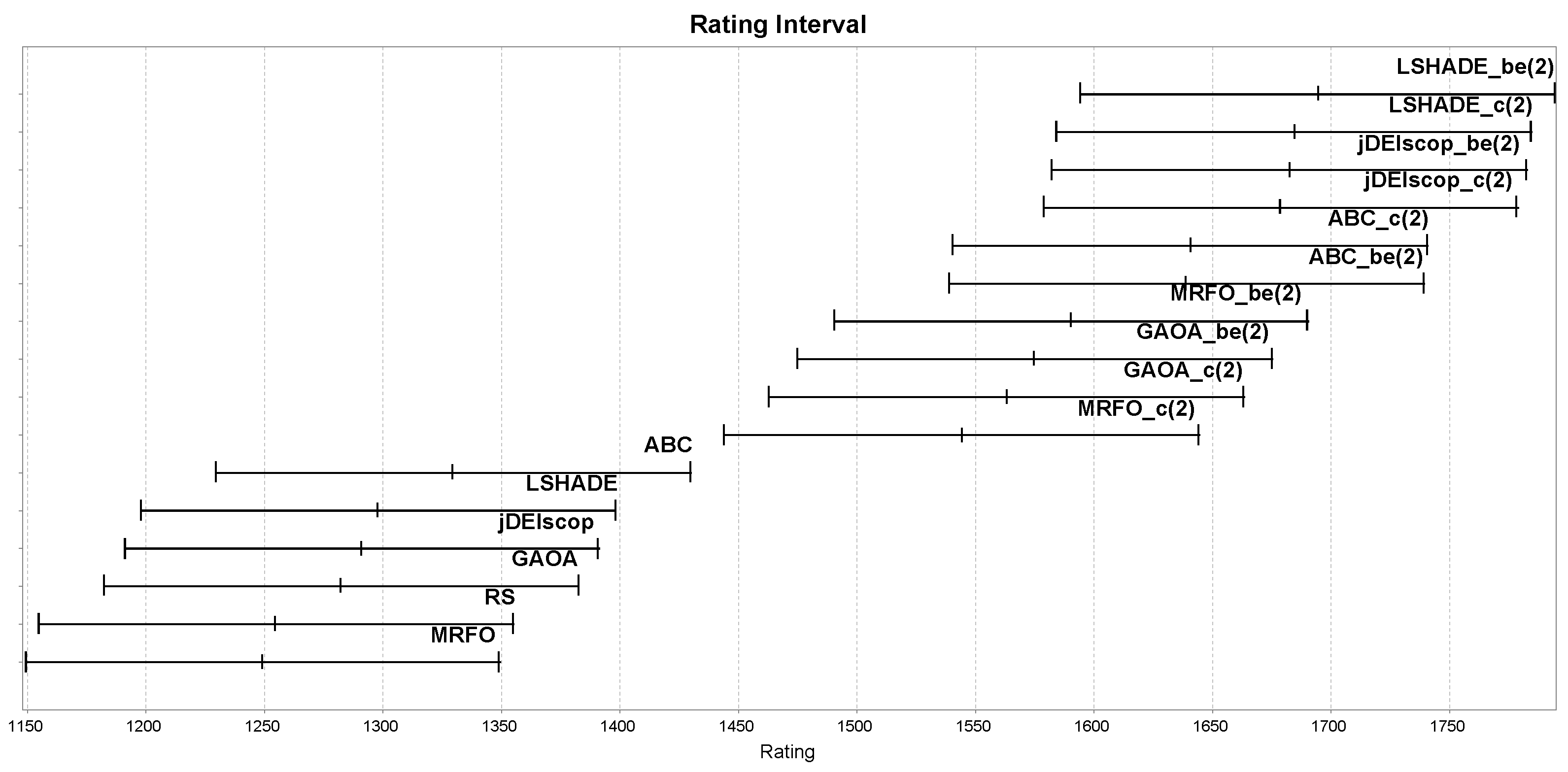
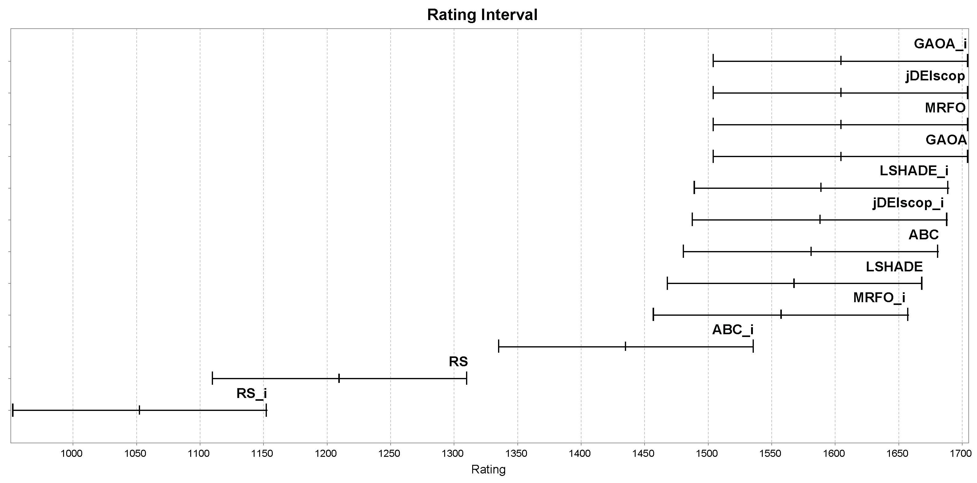
Experiments on the Blind Spot benchmark demonstrated LTMA+’s benefits, with its strategies outperforming LTMA [10] and RS statistically significantly. The top performer, L T M A + b e ( 2 ) , generated random individuals farther from the current best solution and extended the number of such evaluations. The second-best, L T M A + c ( 2 ) , targeted individuals farther from the current duplicate. These results underscore LTMA+’s ability to escape the local optima and enhance search diversity.
Designed as a meta-approach, LTMA+ applies to diverse optimization problems—discrete, continuous, and multi-objective within the EARS framework, where over 60 MAs can be adopted seamlessly. This versatility ensures broad applicability, limited only by inherent search-space constraints, including those that do not sort solutions at the end of the optimization process. Although state-of-the-art MAs are often self-adaptive, dynamically adjusting their control parameters during optimization, our results demonstrate that they can be further enhanced with LTMA+. However, if an MA already incorporates mechanisms similar to LTMA+, significant improvements are not expected.
Moreover, LTMA+ reduces reliance on the algorithm control parameters by enabling self-adaptation to the problem. This is advantageous when the optimal parameters are unknown, minimizing manual tuning and boosting robustness. For instance, if the population size is too small, causing duplicates, LTMA+ generates additional random solutions. While not eliminating parameter tuning entirely, this enhances algorithm robustness.

6.2. The Bad

LTMA+ is an adaptive solution for optimization challenges, including blind spot detection, but its effectiveness diminishes for smaller blind spots or higher problem dimensions. While LTMA+ enhanced MAs’ performance significantly on the Blind Spot benchmark problems, its ability to detect blind spots weakened as the dimensionality increased. At n = 5 , LTMA+-wrapped MAs identified blind spots inconsistently across the runs.
A second concern, especially for experienced users, is the additional computational cost and resources required. LTMA+ demands extra memory to store and manage long-term optimization data, a burden that grows in large-scale problems with many evaluations. While duplicate evaluations do not count toward stopping criteria, searching memory incurs computational time. Solution comparisons are discretized by decimal places, introducing a parameter (Pr) that is primarily problem-dependent (i.e., how much precision makes sense for a solution), but can also be used to tune the optimization process. Edge-case problems are those that require a very high level of precision. In such cases, the LTMA+ approach may be less effective, as the generation of duplicate solutions is less likely, and more memory is required to store potential duplicates.
An efficient LTMA+ implementation achieves near-linear time complexity for duplicate detection and memory operations, enabling optimization speedups for MAs on benchmark problems with blind spots, such as the blind spot suite. The time complexity and resulting speedups of LTMA-wrapped MAs were discussed in detail in the original LTMA study [10], where we showed that the LTMA computation cost was marginal and non-significant. An edge case for computational efficiency includes methods that rarely generate duplicate solutions; an extreme example of this is the RS algorithm. Another partial edge case involves problems where fitness evaluation is very computationally efficient—comparable to a memory lookup in LTMA+. In such cases, the LTMA+ optimization process is slower than running without LTMA+, but it can offer greater robustness, as the detection of duplicate solutions triggers additional exploration.
Furthermore, LTMA+ introduces the parameters Hit and strategy selection, which require careful tuning. Small values yielded improvements in our experiments, but their effectiveness varied with the MAs, control parameters, and problem nature, emphasizing the need for parameter sensitivity and adaptability.

6.3. The Ugly

LTMA+ requires integration with a metaheuristic, achieved here via the EARS framework, which relies on object-oriented programming. Many EA researchers, not being software development experts, may struggle to implement or use such meta-approaches. However, these implementations standardize the structure, easing comparison and evolution.
From a results perspective, long runs with many duplicates risk over-exploration, potentially reducing effectiveness.

7. Conclusions

This paper has introduced LTMA+, a novel approach to addressing the blind spot problem in MAs, where the optimization process becomes trapped in the local optima, failing to locate specific global optima. This challenge impairs MAs’ effectiveness in optimization tasks significantly. By leveraging LTMA+ strategies, MAs mitigate stagnation by dynamically enhancing exploration when duplicate solutions indicate optimization stagnation. LTMA+ redirects its focus to underexplored search-space regions, promoting continuous improvement and robustness in problems with blind spots, such as the Blind Spot benchmark problems.
Despite LTMA+’s universal applicability across optimization challenges, its effectiveness diminishes for smaller blind spots or higher-dimensional problems. To advance LTMA+ research, several key directions warrant exploration. First, evaluating LTMA+ on comprehensive benchmarks, with diverse blind spot configurations and dimensions beyond n = 5 , will assess its scalability and robustness. Specifically, testing adaptive LTMA+ strategies, such as L T M A + b e ( 2 ) , on multimodal and constrained problems could optimize blind spot detection. Second, integrating LTMA+ with hybrid MAs or deep learning techniques may enhance exploration in discrete, continuous, and multi-objective domains, addressing real-world applications like scheduling or neural architecture search. Third, investigating LTMA+’s performance under varying evaluation budgets, from real-time constraints (e.g., autonomous navigation) to extended periods (e.g., structural optimization), will clarify its efficacy in time-sensitive scenarios. Finally, developing new adaptive LTMA+ strategies to guide exploration toward underexplored regions would enhance blind spot detection robustness in high-dimensional benchmark problems. These directions, deferred for brevity, highlight LTMA+’s significant promise. We believe LTMA+ holds substantial potential to enhance the robustness of MA in optimization tasks.

Author Contributions

Conceptualization, M.Č., M.M. and M.R.; investigation, M.Č., M.M. and M.R.; methodology, M.Č.; software, M.Č. and L.M.; validation, M.Č., M.M., L.M. and M.R.; writing, original draft, M.Č., M.M. and M.R.; writing, review and editing, M.Č., M.M., L.M. and M.R. All authors have read and agreed to the published version of the manuscript.

Funding

This research was funded by the Slovenian Research Agency Grant Number P2-0041 (B) and P2-0114.

Data Availability Statement

Publicly available datasets were analyzed in this study. This data can be found here: https://github.com/UM-LPM/EARS, accessed on 8 May 2025.

Acknowledgments

AI-assisted tools were used to improve the English language in this paper.

Conflicts of Interest

The authors declare no conflicts of interest.

Appendix A. Easom and Foxholes Experiment

Appendix A.1. Easom Problem

The Equation (A1) defines the E a s o m minimization problem:
f ( x ) = cos ( x 1 ) cos ( x 2 ) exp ( x 1 π ) 2 + ( x 2 π ) 2 where x [ 100 , 100 ]
Figure A1. Fitness landscape of an Easom problem for n = 2 .
Mathematics 13 01580 g0a1

Appendix A.2. Foxholes Problem (Shekel’s Foxholes Function)

The Equation (A2) defines the F o x h o l e s P r o b l e m minimization problem:
a = 32 16 0 16 32 32 16 0 16 32 32 16 0 16 32 32 16 0 16 32 32 16 0 16 32
b = 32 32 32 32 32 16 16 16 16 16 0 0 0 0 0 16 16 16 16 16 32 32 32 32 32
f ( x , y ) = 1 0.002 + i = 1 25 1 i + ( x a i ) 6 + ( y b i ) 6 where x , y [ 65.536 , 65.536 ]
Figure A2. Fitness landscape of a foxholes problem for n = 2 .
Mathematics 13 01580 g0a2

Appendix A.3. Experiment on Easom and Foxholes

We ran a tournament of selected MAs from Section 2, both with and without LTMA (denoted with the suffix _i, e.g., ABC_i for LTMA+-enhanced ABC), on the Easom and Foxholes problems with n = 2 , using a stopping criterion of M a x F E s = 2000 .
The ratings are shown in Figure A3. Further details on this experiment and the interpretation of its results are provided in Section 3.4.
Figure A3. MAs’ ratings on the Easom and Foxholes benchmark with and without LTMA.
Mathematics 13 01580 g0a3
The results demonstrate that classical optimization problems, such as Easom and Foxholes for n = 2 , are relatively easy to solve using the selected MAs (Figure A3). However, these problems cannot be compared directly to the blind spot problems, for which random search outperformed the selected MAs for n = 2 .

Appendix B. Search-Space Exploration Problem

Appendix B.1. AckleyBS Problem

To gain deeper insights into blind spots and pinpoint regions for improvement, we examined the search space explored by the selected MAs on the AckleyBS problem ( n = 2 ) (Figure A4, Figure A5, Figure A6, Figure A7, Figure A8 and Figure A9).
Figure A4. Search space explored with RS for the AckleyBS problem (gray box represents the blind spot).
Mathematics 13 01580 g0a4
Figure A5. Search space explored with ABC for the AckleyBS problem (gray box represents the blind spot).
Mathematics 13 01580 g0a5
Figure A6. Search space explored with LSHADE for the AckleyBS problem (gray box represents the blind spot).
Mathematics 13 01580 g0a6
Figure A7. Search space explored with GAOA for the AckleyBS problem (gray box represents the blind spot).
Mathematics 13 01580 g0a7
Figure A8. Search space explored with MRFO for the AckleyBS problem (gray box represents the blind spot).
Mathematics 13 01580 g0a8
Figure A9. Search space explored with jDElscop for the AckleyBS problem (gray box represents the blind spot).
Mathematics 13 01580 g0a9

Appendix B.2. SchwefelBS 2.26 Problem

To gain deeper insights into blind spots and pinpoint regions for improvement, we examined the search space explored with the selected MAs on the SchwefelBS 2.26 problem ( n = 2 ) (Figure A10, Figure A11, Figure A12, Figure A13, Figure A14 and Figure A15).
Figure A10. Search space explored with RS for the SchwefelBS 2.26 problem (gray box represents the blind spot).
Mathematics 13 01580 g0a10
Figure A11. Search space explored with ABC for the SchwefelBS 2.26 problem (gray box represents the blind spot).
Mathematics 13 01580 g0a11
Figure A12. Search space explored with LSHADE for the SchwefelBS 2.26 problem (gray box represents the blind spot).
Mathematics 13 01580 g0a12
Figure A13. Search space explored with GAOA for the SchwefelBS 2.26 problem (gray box represents the blind spot).
Mathematics 13 01580 g0a13
Figure A14. Search space explored with MRFO for the SchwefelBS 2.26 problem (gray box represents the blind spot).
Mathematics 13 01580 g0a14
Figure A15. Search space explored with jDElscop for the SchwefelBS 2.26 problem (gray box represents the blind spot).
Mathematics 13 01580 g0a15
The search-space exploration patterns of selected MAs with the SphereBS benchmark problem are presented in Section 3.1.

Appendix C. Analysis of Convergence and Exploration on Blind Spot Benchmark Problems

The typical single-run convergence of selected MAs with LTMA+ on the SphereBS, AckleyBS, and SchwefelBS problems for n = 2 is shown in Figure A16, Figure A17 and Figure A18. The convergence graphs illustrate the optimization process over time, with the y-axis representing the fitness values and the x-axis indicating the number of evaluations. These graphs demonstrate that L T M A + b e ( 2 ) extended the convergence and solution quality significantly compared to standard MAs.
Figure A16. Convergence graph for SphereBS n = 2 .
Mathematics 13 01580 g0a16
Figure A17. Convergence graph for AckleyBS n = 2 .
Mathematics 13 01580 g0a17
Figure A18. Convergence graph for SchwefelBS n = 2 .
Mathematics 13 01580 g0a18

Appendix D. Duplicate Hits Analysis

For each problem and algorithm, we generated histograms based on 100 optimization runs, presented as graphs. The y-axis represents frequency (the number of distinct solutions with the same number of memory hits), and the x-axis shows the hit count. For the SphereBS problem with n = 2 and p r = 3 , Figure A19 displays the histogram for the first 21 duplicate hits, with the frequency truncated at 1000 for clarity due to the high number of unique duplicates at hits 1 and 2. For example, GAOA produced 17,028 unique solutions with H i t = 1 , LSHADE had 4287, ABC had 6981, MRFO had 1043, and jDElscop had 485.
The graph reveals that most solutions have low hit counts, while few have high hits (Figure A19). This might suggest effective search space exploration. However, the unshown tail of the graph (rare high-hit individuals) indicates a few solutions with very high hit counts, for which the total sum of hits is concentrated, potentially signaling entrapment in the local optima. To clarify this, we generated a running sum of hits graph for duplicate creation (Figure A22).
Similar patterns emerged for the AckleyBS and S c h w e f e l B S problems (Figure A20 and Figure A21).
Figure A19. SphereBS n = 2 histogram for p r = 3 with hits 1–21.
Mathematics 13 01580 g0a19
Figure A20. Ackley n = 2 histogram pr = 3 for hits 1–21.
Mathematics 13 01580 g0a20
Figure A21. Schwefel 2.26 n = 2 histogram pr = 3 for hits 1–21.
Mathematics 13 01580 g0a21

Appendix E. Time Analysis of Duplicate Creation

Beyond hit frequency (Hit), the timing of duplicate creation—whether early, mid, or late in the optimization process—is critical. We simulated this by calculating the running sum of duplicates ( D A l l ). This timing indicator can trigger a forced exploration phase.
Visualizing this, we added indicators (the triangle symbol ▲) on the graph to mark fitness improvements at corresponding evaluations (Figure A22, Figure A23 and Figure A24). Significant gaps between these markers may indicate stagnation.
Figure A22. Duplicates’ timeline for SphereBS n = 2 .
Mathematics 13 01580 g0a22
In Figure A22, ABC and GAOA consumed all the available evaluations, while MRFO, LSHADE, and jDElscop stagnated, reaching the secondary stopping criterion D A l l = 4000 . ABC exhibited two exploration spikes, likely due to the scout bee limit parameter re-engaging exploration. For MRFO, LSHADE, and jDElscop, the vertical lines mark where duplicates dominated, with no new solutions generated thereafter.
Figure A23. Duplicates’ timeline for AckleyBS n = 2 .
Mathematics 13 01580 g0a23
For AckleyBS, jDElscop generated many duplicates rarely, suggesting an incomplete or unsuccessful exploitation phase (Figure A23).
Figure A24. Duplicates’ timeline for SchwefelBS n = 2 .
Mathematics 13 01580 g0a24
In Figure A24, only LSHADE entered a high-duplicate phase, indicating that it reached exploitation but became trapped in a local optimum.
Duplicate creation varies with problem complexity, such as higher dimensions. Results for n = 5 are shown in Figure A25, Figure A26 and Figure A27.
Figure A25. Duplicates’ timeline for SphereBS n = 5 .
Mathematics 13 01580 g0a25
Figure A26. Duplicates’ timeline for AckleyBS n = 5 .
Mathematics 13 01580 g0a26
Figure A27. Duplicates’ timeline for SchwefelBS n = 5 .
Mathematics 13 01580 g0a27

Appendix F. The Triangular Distribution

Triangular distribution is defined by the probability density function (PDF). Equation (A3) gives the CDF for the triangular distribution.
F ( x ) = 0 if x < a , ( x a ) 2 ( b a ) ( c a ) if a x < c , 1 ( b x ) 2 ( b a ) ( b c ) if c x b .
For example, suppose we search for a random solution within the interval [ 0 , 10 ] . In that case, we define the parameters as follows: the lower bound a = 0 , the upper bound b = 10 , and the mode c = 7 , which shapes the probability distribution (Figure A28).
Figure A28. The triangular distribution generates a random individual farther away from the selected solution.
Mathematics 13 01580 g0a28

Appendix G. Experiment

Appendix G.1. LTMA+r

Table A1. MAs; success using the LTMA+ strategy r for the SphereBS problem.
AlgorithmnMaxFEs LTMA LTMA + r ( 1 ) LTMA + r ( 2 ) LTMA + r ( 5 )
Fit 3 SR 3 Fit 3 SR 3 Fit 3 SR 3 Fit 3 SR 3
RS22000 1.0
± 0.3
99 1.0
± 0.3
99 1.0
± 0.3
99 1.0
± 0.3
99
ABC22000 0.1
± 0.2
6 0.9
± 0.3
91 0.9
± 0.3
92 0.9
± 0.3
88
GAOA22000 0.1
± 0.3
9 0.7
± 0.4
76 0.4
± 0.5
41 0.4
± 0.5
42
MRFO22000 0.2
± 0.4
18 1.0
± 0.1
99 0.9
± 0.2
95 1.0
± 0.2
96
LSHADE22000 0.1
± 0.3
7 0.9
± 0.3
89 0.9
± 0.3
90 0.9
± 0.3
93
jDElscop22000 0.4
± 0.5
37 0.8
± 0.4
78 0.4
± 0.5
45 0.5
± 0.5
48
RS36000 28.8
± 34.7
37 19.8
± 32.0
57 19.6
± 27.6
52 25.1
± 33.3
47
ABC36000 0.0
± 0.0
0 0.3
± 0.5
32 0.2
± 0.4
18 0.2
± 0.4
21
GAOA36000 0.0
± 0.2
5 0.2
± 0.4
24 0.3
± 0.5
29 0.3
± 0.5
32
MRFO36000 0.0
± 0.2
4 0.5
± 0.5
46 0.5
± 0.5
47 0.4
± 0.5
40
LSHADE36000 0.0
± 0.0
0 0.4
± 0.5
39 0.5
± 0.5
46 0.4
± 0.5
44
jDElscop36000 0.0
± 0.1
1 0.2
± 0.4
23 0.2
± 0.4
24 0.2
± 0.4
18
RS48000 177.4
± 94.4
3 161.1
± 104.6
8 169.7
± 101.4
5 173.6
± 103.3
1
ABC48000 0.0
± 0.0
0 0.0
± 0.1
1 0.0
± 0.0
0 0.0
± 0.0
0
GAOA48000 0.1
± 0.3
12 0.0
± 0.0
0 0.0
± 0.2
4 0.0
± 0.1
1
MRFO48000 0.0
± 0.0
0 0.1
± 0.2
6 0.1
± 0.2
6 0.0
± 0.1
2
LSHADE48000 0.0
± 0.0
0 0.0
± 0.2
5 0.0
± 0.2
3 0.0
± 0.2
3
jDElscop48000 0.0
± 0.0
0 0.0
± 0.1
1 0.0
± 0.2
3 0.0
± 0.1
1
RS510,000 449.9
± 193.4
1 442.7
± 210.7
0 438.5
± 200.6
2 494.6
± 208.0
2
ABC510,000 0.0
± 0.0
0 0.0
± 0.0
0 0.0
± 0.1
1 0.0
± 0.0
0
GAOA510,000 0.2
± 0.4
19 0.0
± 0.0
0 0.0
± 0.1
1 0.0
± 0.0
0
MRFO510,000 0.0
± 0.0
0 0.0
± 0.0
0 0.0
± 0.0
0 0.0
± 0.0
0
LSHADE510,000 0.0
± 0.0
0 0.0
± 0.0
0 0.0
± 0.0
0 0.0
± 0.1
2
jDElscop510,000 0.0
± 0.0
0 0.0
± 0.0
0 0.0
± 0.0
0 0.0
± 0.0
0
Table A2. MAs’ success using the LTMA+ strategy r for the SchwefelBS 2.26 problem.
AlgorithmnMaxFEs LTMA LTMA + r ( 1 ) LTMA + r ( 2 ) LTMA + r ( 5 )
Fit 3 SR 3 Fit 3 SR 3 Fit 3 SR 3 Fit 3 SR 3
RS22000 838.8
± 1.8
99 838.8
± 1.8
99 838.8
± 1.8
99 838.8
± 1.8
99
ABC22000 838.0
± 0.3
5 838.8
± 0.4
80 838.7
± 0.4
76 838.6
± 0.5
67
GAOA22000 837.5
± 6.5
60 838.3
± 1.5
71 838.3
± 1.1
62 837.9
± 2.4
64
MRFO22000 812.2
± 49.4
33 831.0
± 28.4
67 834.9
± 20.4
69 830.2
± 30.6
67
LSHADE22000 816.7
± 45.8
9 838.8
± 0.4
79 837.6
± 11.9
79 838.7
± 0.4
78
jDElscop22000 833.6
± 9.6
53 838.5
± 0.5
56 835.5
± 8.7
73 834.8
± 9.7
71
RS36000 1206.5
± 69.6
55 1214.9
± 62.7
58 1201.8
± 72.1
48 1200.7
± 70.2
50
ABC36000 1256.9
± 0.0
0 1257.1
± 0.4
20 1257.2
± 0.4
23 1257.2
± 0.4
23
GAOA36000 1246.1
± 28.1
3 1251.2
± 18.0
11 1247.3
± 24.5
6 1249.5
± 19.7
8
MRFO36000 1147.2
± 96.0
8 1189.3
± 76.3
13 1178.0
± 80.5
13 1184.9
± 76.5
16
LSHADE36000 1214.3
± 66.3
0 1247.9
± 32.4
39 1241.8
± 40.1
23 1245.5
± 35.8
40
jDElscop36000 1252.9
± 5.2
1 1257.1
± 0.4
15 1252.8
± 5.4
2 1252.9
± 4.9
6
RS48000 1384.7
± 83.0
2 1396.4
± 101.4
4 1382.1
± 77.2
0 1425.8
± 120.0
8
ABC48000 1675.9
± 0.0
0 1676.0
± 0.1
2 1675.9
± 0.0
0 1675.5
± 4.2
1
GAOA48000 1620.0
± 52.0
1 1620.9
± 59.8
0 1620.0
± 55.9
2 1614.9
± 52.3
1
MRFO48000 1448.2
± 128.3
0 1463.4
± 123.2
1 1492.1
± 122.2
3 1456.6
± 137.9
0
LSHADE48000 1617.9
± 85.0
0 1621.5
± 68.3
5 1621.5
± 74.2
1 1621.5
± 72.3
5
jDElscop48000 1653.2
± 23.0
0 1675.9
± 0.1
1 1651.9
± 24.7
0 1653.8
± 23.8
0
RS510,000 1582.5
± 106.1
0 1602.8
± 99.0
0 1601.7
± 116.9
1 1596.3
± 103.9
0
ABC510,000 2094.9
± 0.0
0 2094.6
± 3.0
0 2094.9
± 0.1
0 2093.7
± 11.8
0
GAOA510,000 1955.5
± 66.7
0 1963.1
± 78.5
0 1949.7
± 76.4
0 1972.4
± 68.5
0
MRFO510,000 1748.7
± 195.3
0 1755.2
± 163.7
0 1764.0
± 179.8
0 1738.8
± 184.9
0
LSHADE510,000 2039.2
± 72.3
0 2033.3
± 81.6
0 2035.7
± 78.1
0 2029.8
± 83.1
1
jDElscop510,000 2047.4
± 35.4
0 2094.9
± 0.0
0 2039.2
± 44.5
0 2044.7
± 38.8
0

Appendix G.2. LTMA+c

Table A3. MAs’ success using the LTMA+ strategy c for the SphereBS Problem.
AlgorithmnMaxFEs LTMA LTMA + c ( 1 ) LTMA + c ( 2 ) LTMA + r ( 5 )
Fit 3 SR 3 Fit 3 SR 3 Fit 3 SR 3 Fit 3 SR 3
RS22000 1.0
± 0.3
99 1.0
± 0.3
99 1.0
± 0.2
100 1.0
± 0.4
99
ABC22000 0.1
± 0.2
6 1.0
± 0
100 1.0
± 0
100 1.0
± 0
100
GAOA22000 0.1
± 0.3
9 1.0
± 0
100 1.0
± 0.1
98 0.9
± 0.3
90
MRFO22000 0.2
± 0.4
18 1.0
± 0
100 1.0
± 0
100 1.0
± 0
100
LSHADE22000 0.1
± 0.3
7 1.0
± 0
100 1.0
± 0
100 1.0
± 0
100
jDElscop22000 0.4
± 0.5
37 1.0
± 0
100 0.8
± 0.4
77 0.7
± 0.5
69
RS36000 28.8
± 34.7
37 24.1
± 31.6
47 22.2
± 30.3
47 21.7
± 30.0
48
ABC36000 0.0
± 0.0
0 1.0
± 0.1
99 1.0
± 0.1
100 1.0
± 0.1
100
GAOA36000 0.0
± 0.2
5 1.0
± 0
100 1.0
± 0.1
100 1.0
± 0.1
99
MRFO36000 0.0
± 0.2
4 1.0
± 0
100 1.0
± 0
100 1.0
± 0
100
LSHADE36000 0.0
± 0.0
0 1.0
± 0
100 1.0
± 0
100 1.0
± 0
100
jDElscop36000 0.0
± 0.1
1 1.0
± 0
100 0.9
± 0.2
94 0.9
± 0.3
91
RS48000 177.4
± 94.4
3 158.4
± 97.9
8 158.0
± 92.9
7 162.9
± 93.4
6
ABC48000 0.0
± 0.0
0 0.7
± 0.5
67 0.7
± 0.5
67 0.7
± 0.5
66
GAOA48000 0.1
± 0.3
12 0.7
± 0.4
75 0.8
± 0.4
79 0.8
± 0.4
77
MRFO48000 0.0
± 0.0
0 0.9
± 0.3
93 0.9
± 0.3
93 0.9
± 0.3
93
LSHADE48000 0.0
± 0.0
0 0.9
± 0.2
95 0.9
± 0.3
92 0.9
± 0.3
91
jDElscop48000 0.0
± 0.0
0 0.7
± 0.4
73 0.7
± 0.5
66 0.7
± 0.5
65
RS510,000 449.9
± 193.4
1 465.4
± 233.1
1 480.2
± 213.1
1 472.4
± 205.8
1
ABC510,000 0.0
± 0.0
0 0.1
± 0.4
15 0.2
± 0.4
16 0.2
± 0.4
15
GAOA510,000 0.2
± 0.4
19 0.2
± 0.4
20 0.3
± 0.4
26 0.2
± 0.4
23
MRFO510,000 0.0
± 0.0
0 0.3
± 0.5
35 0.4
± 0.5
36 0.4
± 0.5
38
LSHADE510,000 0.0
± 0.0
0 0.3
± 0.5
35 0.4
± 0.5
37 0.4
± 0.5
38
jDElscop510,000 0.0
± 0.0
0 0.2
± 0.4
22 0.2
± 0.4
17 0.2
± 0.4
16
Table A4. MAs’ success using the LTMA+ strategy c for the SchwefelBS 2.26 problem.
AlgorithmnMaxFEs LTMA LTMA + c ( 1 ) LTMA + c ( 2 ) LTMA + r ( 5 )
Fit 3 SR 3 Fit 3 SR 3 Fit 3 SR 3 Fit 3 SR 3
RS22000 838.8
± 1.8
99 838.8
± 1.8
99 838.8
± 1.8
99 838.8
± 1.8
99
ABC22000 838.0
± 0.3
5 839.0
± 0
100 839.0
± 0.1
99 839.0
± 0.1
99
GAOA22000 837.5
± 6.5
60 838.9
± 0.3
96 838.8
± 0.5
90 836.9
± 12.0
61
MRFO22000 812.2
± 49.4
33 820.1
± 43.1
80 819.7
± 43.9
76 817.3
± 46.3
79
LSHADE22000 816.7
± 45.8
9 839.0
± 0
100 839.0
± 0
100 839.0
± 0
100
jDElscop22000 833.6
± 9.6
53 838.8
± 0.4
81 836.8
± 6.0
79 836.8
± 6.7
83
RS36000 1206.5
± 69.6
55 1214.9
± 64.0
59 1219.6
± 61.8
64 1210.8
± 67.3
58
ABC36000 1256.9
± 0.0
0 1257.9
± 0.2
95 1257.9
± 0.2
97 1257.8
± 0.4
84
GAOA36000 1246.1
± 28.1
3 1256.3
± 5.4
53 1252.2
± 17.8
46 1246.7
± 25.5
18
MRFO36000 1147.2
± 96.0
8 1189.0
± 82.2
45 1186.0
± 81.3
31 1192.4
± 76.7
28
LSHADE36000 1214.3
± 66.3
0 1257.9
± 0
100 1257.9
± 0
100 1257.9
± 0
100
jDElscop36000 1252.9
± 5.2
1 1257.8
± 0.3
88 1253.3
± 6.5
8 1252.4
± 11.2
4
RS48000 1384.7
± 83.0
2 1416.2
± 108.9
6 1412.1
± 112.7
7 1413.1
± 105.2
4
ABC48000 1675.9
± 0.0
0 1676.3
± 0.5
34 1676.3
± 0.5
37 1676.2
± 0.5
28
GAOA48000 1620.0
± 52.0
1 1627.5
± 53.3
12 1623.1
± 52.0
10 1628.1
± 52.0
3
MRFO48000 1448.2
± 128.3
0 1463.1
± 130.2
7 1478.4
± 125.9
7 1474.7
± 132.8
3
LSHADE48000 1617.9
± 85.0
0 1661.2
± 40.3
68 1669.5
± 28.4
65 1663.6
± 44.4
68
jDElscop48000 1653.2
± 23.0
0 1675.0
± 11.9
23 1654.7
± 24.0
0 1656.1
± 17.9
0
RS510,000 1582.5
± 106.1
0 1588.1
± 82.7
0 1619.1
± 119.3
1 1584.3
± 91.1
0
ABC510,000 2094.9
± 0.0
0 2095.0
± 0.2
5 2093.4
± 12.7
10 2094.9
± 0.3
3
GAOA510,000 1955.5
± 66.7
0 1984.7
± 78.8
0 1954.0
± 73.2
1 1966.1
± 68.1
0
MRFO510,000 1748.7
± 195.3
0 1805.9
± 183.8
5 1749.8
± 178.2
1 1755.6
± 148.1
0
LSHADE510,000 2039.2
± 72.3
0 2043.0
± 76.0
19 2035.8
± 78.2
14 2032.3
± 85.1
17
jDElscop510,000 2047.4
± 35.4
0 2094.9
± 0.2
3 2043.8
± 44.1
0 2043.0
± 41.0
0

Appendix G.3. LTMA+b

Table A5. MAs’ success using the LTMA+ strategy b for the SphereBS problem.
AlgorithmnMaxFEs LTMA LTMA + b ( 1 ) LTMA + b ( 2 ) LTMA + b ( 5 )
Fit 3 SR 3 Fit 3 SR 3 Fit 3 SR 3 Fit 3 SR 3
RS22000 1.0
± 0.3
99 1.0
± 0.3
99 1.0
± 0.3
99 1.0
± 0.3
99
ABC22000 0.1
± 0.2
6 1.0
± 0
100 1.0
± 0
100 1.0
± 0
100
GAOA22000 0.1
± 0.3
9 1.0
± 0.2
100 0.9
± 0.3
90 0.6
± 0.5
70
MRFO22000 0.2
± 0.4
18 1.0
± 0
100 1.0
± 0
100 1.0
± 0
100
LSHADE22000 0.1
± 0.3
7 1.0
± 0
100 1.0
± 0
100 1.0
± 0
100
jDElscop22000 0.4
± 0.5
37 1.0
± 0
100 0.5
± 0.5
49 0.5
± 0.5
50
RS36000 28.8
± 34.7
37 21.0
± 32.2
51 18.6
± 26.7
56 16.8
± 24.5
54
ABC36000 0.0
± 0.0
0 1.0
± 0
100 1.0
± 0.1
99 1.0
± 0
100
GAOA36000 0.0
± 0.2
5 1.0
± 0
100 1.0
± 0.1
99 1.0
± 0.2
97
MRFO36000 0.0
± 0.2
4 1.0
± 0
100 1.0
± 0
100 1.0
± 0
100
LSHADE36000 0.0
± 0.0
0 1.0
± 0
100 1.0
± 0
100 1.0
± 0
100
jDElscop36000 0.0
± 0.1
1 1.0
± 0
100 0.9
± 0.3
88 0.9
± 0.3
86
RS48000 177.4
± 94.4
3 185.3
± 107.9
6 166.3
± 99.4
5 172.6
± 97.2
6
ABC48000 0.0
± 0.0
0 0.7
± 0.5
72 0.7
± 0.5
68 0.6
± 0.5
61
GAOA48000 0.1
± 0.3
12 0.8
± 0.4
77 0.7
± 0.5
71 0.8
± 0.4
79
MRFO48000 0.0
± 0.0
0 0.9
± 0.2
94 0.9
± 0.2
95 0.9
± 0.3
89
LSHADE48000 0.0
± 0.0
0 1.0
± 0.2
96 0.9
± 0.3
92 0.9
± 0.3
89
jDElscop48000 0.0
± 0.0
0 0.8
± 0.4
82 0.6
± 0.5
61 0.6
± 0.5
58
RS510,000 449.9
± 193.4
1 484.5
± 194.9
1 458.9
± 197.4
0 471.0
± 212.0
0
ABC510,000 0.0
± 0.0
0 0.1
± 0.4
15 0.2
± 0.4
19 0.2
± 0.4
16
GAOA510,000 0.2
± 0.4
19 0.2
± 0.4
25 0.2
± 0.4
25 0.2
± 0.4
20
MRFO510,000 0.0
± 0.0
0 0.4
± 0.5
36 0.3
± 0.5
34 0.3
± 0.5
29
LSHADE510,000 0.0
± 0.0
0 0.3
± 0.5
34 0.3
± 0.5
34 0.4
± 0.5
37
jDElscop510,000 0.0
± 0.0
0 0.2
± 0.4
20 0.2
± 0.4
16 0.2
± 0.4
18
Table A6. MAs’ success using the LTMA+ strategy b for the SchwefelBS 2.26 problem.
AlgorithmnMaxFEs LTMA LTMA + b ( 1 ) LTMA + b ( 2 ) LTMA + b ( 5 )
Fit 3 SR 3 Fit 3 SR 3 Fit 3 SR 3 Fit 3 SR 3
RS22000 838.8
± 1.8
99 838.8
± 1.8
99 838.8
± 1.8
99 838.8
± 1.8
99
ABC22000 838.0
± 0.3
5 839.0
± 0
100 839.0
± 0
100 839.0
± 0.1
99
GAOA22000 837.5
± 6.5
60 838.9
± 0.4
99 838.9
± 0.4
98 838.8
± 0.6
92
MRFO22000 812.2
± 49.4
33 838.9
± 0.1
98 839.0
± 0
100 839.0
± 0
100
LSHADE22000 816.7
± 45.8
9 839.0
± 0
100 839.0
± 0
100 839.0
± 0
100
jDElscop22000 833.6
± 9.6
53 838.9
± 0.3
92 838.5
± 2.0
93 837.6
± 4.8
89
RS36000 1206.5
± 69.6
55 1204.7
± 70.2
49 1209.5
± 60.3
47 1202.3
± 66.9
50
ABC36000 1256.9
± 0.0
0 1257.9
± 0.2
97 1257.8
± 0.3
88 1257.8
± 0.4
84
GAOA36000 1246.1
± 28.1
3 1254.8
± 9.9
65 1251.8
± 13.7
40 1252.3
± 14.8
25
MRFO36000 1147.2
± 96.0
8 1222.5
± 78.0
65 1213.5
± 80.9
62 1236.7
± 55.7
73
LSHADE36000 1214.3
± 66.3
0 1257.9
± 0.1
99 1257.9
± 0
100 1257.9
± 0
100
jDElscop36000 1252.9
± 5.2
1 1257.8
± 0.4
83 1253.5
± 6.1
24 1252.5
± 7.6
21
RS48000 1384.7
± 83.0
2 1394.5
± 105.0
6 1411.4
± 117.3
6 1422.6
± 121.3
10
ABC48000 1675.9
± 0.0
0 1676.3
± 0.5
41 1676.3
± 0.5
32 1676.1
± 0.4
18
GAOA48000 1620.0
± 52.0
1 1636.3
± 53.4
14 1614.4
± 55.5
12 1616.5
± 55.5
1
MRFO48000 1448.2
± 128.3
0 1495.7
± 138.5
18 1478.2
± 140.1
11 1476.5
± 140.3
12
LSHADE48000 1617.9
± 85.0
0 1674.3
± 16.8
71 1667.1
± 32.5
66 1663.5
± 37.5
59
jDElscop48000 1653.2
± 23.0
0 1676.1
± 0.4
20 1652.5
± 25.6
4 1654.2
± 19.4
0
RS510,000 1582.5
± 106.1
0 1594.4
± 112.7
0 1612.7
± 121.6
1 1594.6
± 113.5
0
ABC510,000 2094.9
± 0.0
0 2093.8
± 11.9
5 2093.8
± 11.9
6 2095.0
± 0.3
7
GAOA510,000 1955.5
± 66.7
0 1977.4
± 68.2
1 1957.3
± 77.3
1 1958.8
± 73.0
0
MRFO510,000 1748.7
± 195.3
0 1746.0
± 162.0
1 1765.1
± 168.6
0 1782.5
± 173.0
3
LSHADE510,000 2039.2
± 72.3
0 2038.2
± 83.4
15 2033.5
± 88.4
18 2041.8
± 84.9
14
jDElscop510,000 2047.4
± 35.4
0 2092.5
± 16.7
0 2034.3
± 38.5
0 2044.5
± 40.3
0

Appendix G.4. LTMA+be

Table A7. MAs’ success using the LTMA+ strategy b e for the SphereBS problem.
AlgorithmnMaxFEs LTMA LTMA + be ( 1 ) LTMA + be ( 2 ) LTMA + be ( 5 )
Fit 3 SR 3 Fit 3 SR 3 Fit 3 SR 3 Fit 3 SR 3
RS22000 1.0
± 0.1
99 1.0
± 0.3
99 1.0
± 0.2
100 1.0
± 0.2
100
ABC22000 0.1
± 0.3
10 1.0
± 0
100 1.0
± 0
100 1.0
± 0
100
GWO22000 0.0
± 0.0
3 1.0
± 0
99 1.0
± 0
100 1.0
± 0
99
GAOA22000 0.1
± 0.4
20 1.0
± 0.2
99 0.9
± 0.3
95 0.9
± 0.3
90
MRFO22000 0.3
± 0.5
35 1.0
± 0
100 1.0
± 0
100 1.0
± 0
100
LSHADE22000 0.1
± 0.3
10 1.0
± 0
100 1.0
± 0
100 1.0
± 0
100
jDElscop22000 0.4
± 0.5
38 1.0
± 0
100 0.7
± 0.4
75 0.7
± 0.5
70
RS36000 22.4
± 29.7
42 16.1
± 28.1
57 16.5
± 26.5
55 16.5
± 25.7
54
ABC36000 0.0
± 0.0
0 1.0
± 0
100 1.0
± 0
100 1.0
± 0
100
GWO36000 0.0
± 0.0
0 1.0
± 0
81 1.0
± 0
71 1.0
± 0
67
GAOA36000 0.0
± 0.2
5 1.0
± 0
100 1.0
± 0
100 1.0
± 0
100
MRFO36000 0.0
± 0.1
2 1.0
± 0
100 1.0
± 0
100 1.0
± 0
100
LSHADE36000 0.0
± 0.1
2 1.0
± 0
100 1.0
± 0
100 1.0
± 0
100
jDElscop36000 0.0
± 0.2
3 1.0
± 0
100 1.0
± 0.2
96 0.9
± 0.2
94
RS48000 149.0
± 90.7
9 177.1
± 106.7
5 168.6
± 102.9
7 163.5
± 99.2
6
ABC48000 0.0
± 0.0
0 0.8
± 0.4
84 0.8
± 0.4
84 0.8
± 0.4
80
GWO48000 0.0
± 0.0
0 1.0
± 0
18 1.0
± 0
20 1.0
± 0
18
GAOA48000 0.1
± 0.3
14 0.8
± 0.4
82 0.8
± 0.4
80 0.8
± 0.4
77
MRFO48000 0.0
± 0.0
0 1.0
± 0.1
98 0.9
± 0.2
95 0.9
± 0.2
94
LSHADE48000 0.0
± 0.0
0 0.9
± 0.3
91 0.9
± 0.2
95 1.0
± 0.2
95
jDElscop48000 0.0
± 0.0
0 0.8
± 0.4
76 0.7
± 0.5
69 0.7
± 0.5
67
RS510,000 459.5
± 219.2
2 487.2
± 201.1
0 466.7
± 194.8
0 470.2
± 185.8
0
ABC510,000 0.0
± 0.0
0 0.3
± 0.5
33 0.3
± 0.5
33 0.3
± 0.5
28
GWO510,000 0.0
± 0.0
0 1.0
± 0
5 1.0
± 0
3 1.0
± 0
3
GAOA510,000 0.2
± 0.4
19 0.3
± 0.5
32 0.3
± 0.5
32 0.3
± 0.5
30
MRFO510,000 0.0
± 0.0
0 0.4
± 0.5
40 0.4
± 0.5
43 0.4
± 0.5
45
LSHADE510,000 0.0
± 0.0
0 0.3
± 0.5
34 0.3
± 0.5
34 0.4
± 0.5
37
jDElscop510,000 0.0
± 0.0
0 0.2
± 0.4
19 0.2
± 0.4
20 0.2
± 0.4
18
Table A8. MAs’ success using the LTMA+ strategy b e for the SchwefelBS 2.26 problem.
AlgorithmnMaxFEs LTMA LTMA + be ( 1 ) LTMA + be ( 2 ) LTMA + be ( 5 )
Fit 3 SR 3 Fit 3 SR 3 Fit 3 SR 3 Fit 3 SR 3
RS22000 839.0
± 0
100 838.8
± 1.8
99 838.8
± 1.5
99 838.8
± 2.0
99
ABC22000 838.1
± 0.3
9 839.0
± 0
100 839.0
± 0
100 839.0
± 0.1
99
GWO22000 609.9
± 143.7
21 839.0
± 0
44 1210.0
± 371.9
42 1380.2
± 387.6
41
GAOA22000 837.8
± 2.4
54 838.9
± 0.1
99 838.9
± 0.2
98 838.9
± 0.5
95
MRFO22000 812.1
± 49.4
30 839.0
± 0
100 839.0
± 0.1
100 839.0
± 0.1
100
LSHADE22000 822.6
± 40.1
7 839.0
± 0
100 839.0
± 0
100 839.0
± 0
100
jDElscop22000 836.3
± 5.3
61 838.9
± 0.3
90 838.6
± 1.8
92 838.3
± 3.7
91
RS36000 1186.8
± 68.1
39 1210.2
± 68.8
61 1203.8
± 69.6
54 1202.0
± 69.3
52
ABC36000 1256.9
± 0.0
0 1257.9
± 0
100 1257.9
± 0.1
100 1257.9
± 0.1
99
GWO36000 577.4
± 161.1
2 1249.6
± 43.6
4 1415.2
± 168.9
5 1517.0
± 199.5
5
GAOA36000 1243.4
± 31.8
4 1256.9
± 9.0
93 1257.0
± 6.6
89 1257.0
± 5.5
82
MRFO36000 1138.2
± 97.3
5 1243.6
± 51.8
89 1243.5
± 53.0
89 1245.5
± 49.8
91
LSHADE36000 1209.6
± 65.2
1 1257.9
± 0
100 1257.9
± 0
100 1257.9
± 0.1
99
jDElscop36000 1253.9
± 4.4
7 1257.9
± 0.3
93 1255.8
± 7.2
76 1254.9
± 8.6
69
RS48000 1391.2
± 88.4
2 1408.6
± 97.2
5 1394.5
± 105.3
5 1399.2
± 100.4
4
ABC48000 1675.9
± 0.0
0 1676.6
± 0.5
67 1676.5
± 0.5
59 1676.4
± 0.5
52
GWO48000 568.1
± 166.7
0 1309.1
± 17.9
0 1445.0
± 136.9
0 1536.9
± 171.5
0
GAOA48000 1621.1
± 54.3
0 1636.1
± 55.7
27 1630.5
± 59.5
27 1626.9
± 57.8
21
MRFO48000 1447.3
± 144.1
2 1560.4
± 121.7
30 1544.1
± 128.2
27 1550.6
± 127.0
29
LSHADE48000 1630.9
± 66.9
0 1670.7
± 26.1
73 1670.7
± 26.0
70 1669.5
± 28.4
69
jDElscop48000 1654.8
± 16.7
0 1676.1
± 0.4
18 1662.5
± 27.6
12 1658.7
± 26.3
8
RS510,000 1594.2
± 111.1
1 1582.6
± 117.8
1 1588.9
± 120.2
1 1594.8
± 116.9
1
ABC510,000 2094.9
± 0.0
0 2095.0
± 0.4
13 2094.4
± 8.4
14 2094.6
± 6.9
12
GWO510,000 574.6
± 158.8
0 1542.0
± 69.1
0 1599.9
± 90.4
0 1640.1
± 93.2
0
GAOA510,000 1950.2
± 70.3
0 1949.7
± 90.5
10 1942.3
± 93.9
7 1951.1
± 89.5
7
MRFO510,000 1738.0
± 181.9
0 1826.7
± 158.6
3 1824.3
± 159.9
3 1810.6
± 163.2
3
LSHADE510,000 2020.3
± 99.1
0 2058.4
± 62.4
18 2054.8
± 68.8
17 2055.2
± 67.6
17
jDElscop510,000 2041.0
± 39.0
0 2094.9
± 0.1
2 2059.8
± 50.4
2 2053.3
± 49.9
1

Appendix G.5. Evaluating LTMA+ on Benchmarks Without Blind Spots

For a thorough comparison with the original LTMA method, we selected two test cases from the original LTMA paper: the CEC’15 benchmark problem (Experiment 2) and the real-world soil problem (Experiment 3) [10]. We set the Hit parameter to 12, using benchmark problems with n = 10 and MaxFEs = 10 , 000 . The LTMA memory precision (Pr) was set to 9.
As the LTMA+ strategies are intended to improve performance primarily in scenarios with blind spots, no substantial differences were expected on these benchmark problems. Nonetheless, it was important to verify that the LTMA+ strategies do not impact the performance of the original LTMA method negatively.
We employed the CRS4EAs rating system for statistical analysis, as described in Section 3.4 [54,55]. To simulate LTMA, we used the following strategy variants: LTMA + c ( 12 ) , LTMA + b e ( 12 ) , and LTMA + i .

CEC’15 Benchmark

The CEC’15 benchmark comprises a widely recognized collection of test functions designed to assess optimization algorithm performance [27]. For our evaluation, we used a problem dimensionality of n = 10 and a maximum of MaxFEs = 10 , 000 function evaluations. These benchmark functions include unimodal functions to test convergence speed, multimodal functions with multiple local optima to challenge exploration, rotated functions to assess the handling of non-separable variables, and composite functions combining multiple properties for complex optimization scenarios.
Figure A29. MAs’ algorithm ratings on the CEC’15 benchmark.
Mathematics 13 01580 g0a29
Figure A29 demonstrates that the LTMA+ strategies did not exhibit significant differences in performance compared to the original LTMA.

Appendix G.6. Soil Model Optimization Problems

The real-world optimization task involves estimating the parameters of a three-layer soil model, specifically the thicknesses ( h 1 , h 2 ) and resistivities ( p 1 , p 2 , p 3 ) of the layers [56,57]. These parameters are essential for the accurate dimensioning of grounding systems using the finite element method (FEM), which ensures safety during electrical faults or lightning strikes.
To determine these parameters, resistivity measurements were conducted using the Wenner four-electrode method [58], where the apparent resistivity is computed based on electrode spacing and measured voltage/current. The optimization goal is to minimize the error between the measured and model-computed apparent resistivities. The fitness function is defined as the mean relative error over all the measurement points (Equation (A4)).
F fitness = 1 n i = 1 n p i c p i m p i m · 100 ( % )
Three data sets (TE1, TE2, and TE3) were used as separate problem instances. The analytical solution for apparent resistivity is based on Bessel function integrals, approximated via numerical integration with a cutoff at λ max . More details about the problem and the data sets can be found in [10,57].
Figure A30, Figure A31 and Figure A32 demonstrate that the LTMA+ strategies did not exhibit significant differences in performance compared to the original LTMA on benchmarks without blind spots.
Figure A30. MAs’ ratings on the soil problem—TE1 Data Set.
Mathematics 13 01580 g0a30
Figure A31. MAs’ ratings on the soil problem—TE2 Data Set.
Mathematics 13 01580 g0a31
Figure A32. MAs’ ratings on the soil problem—TE3 Data Set.
Mathematics 13 01580 g0a32

References

  1. Tsai, C.; Chiang, M. Handbook of Metaheuristic Algorithms: From Fundamental Theories to Advanced Applications; Elsevier: Amsterdam, The Netherlands, 2023. [Google Scholar]
  2. Črepinšek, M.; Liu, S.H.; Mernik, M. Replication and comparison of computational experiments in applied evolutionary computing: Common pitfalls and guidelines to avoid them. Appl. Soft Comput. 2014, 19, 161–170. [Google Scholar] [CrossRef]
  3. Deng, L.; Liu, S. Metaheuristics exposed: Unmasking the design pitfalls of arithmetic optimization algorithm in benchmarking. Swarm Evol. Comput. 2024, 86, 101535. [Google Scholar] [CrossRef]
  4. Taleb, N.N. The Black Swan: The Impact of the Highly Improbable; Random House: New York, NY, USA, 2007. [Google Scholar]
  5. Taleb, N. Antifragile: Things That Gain from Disorder; Incerto; Random House Publishing Group: Westminster, MD, USA, 2012. [Google Scholar]
  6. Taleb, N.N. Skin in the Game: Hidden Asymmetries in Daily Life; Random House: New York, NY, USA, 2018. [Google Scholar]
  7. Hansen, N.; Ostermeier, A. Completely derandomized self-adaptation in evolution strategies. Evol. Comput. 2001, 9, 159–195. [Google Scholar] [CrossRef]
  8. Hsieh, F.S. A Self-Adaptive Meta-Heuristic Algorithm Based on Success Rate and Differential Evolution for Improving the Performance of Ridesharing Systems with a Discount Guarantee. Algorithms 2024, 17, 9. [Google Scholar] [CrossRef]
  9. Piotrowski, A.P. Review of Differential Evolution population size. Swarm Evol. Comput. 2017, 32, 1–24. [Google Scholar] [CrossRef]
  10. Črepinšek, M.; Liu, S.H.; Mernik, M.; Ravber, M. Long Term Memory Assistance for Evolutionary Algorithms. Mathematics 2019, 7, 1129. [Google Scholar] [CrossRef]
  11. Holland, J.H. Adaptation in Natural and Artificial Systems; University of Michigan Press: Ann Arbor, MI, USA, 1975; Reprinted by MIT Press: Cambridge, MA, USA, 1992. [Google Scholar]
  12. Eiben, A.E.; Smith, J.E. Introduction to Evolutionary Computing; Natural Computing Series; Springer: Berlin/Heidelberg, Germany, 2003. [Google Scholar]
  13. Zhan, Z.H.; Shi, L.; Tan, K.C.; Zhang, J. A survey on evolutionary computation for complex continuous optimization. Artif. Intell. Rev. 2022, 55, 59–110. [Google Scholar] [CrossRef]
  14. Jerebic, J.; Mernik, M.; Liu, S.H.; Ravber, M.; Baketarić, M.; Mernik, L.; Črepinšek, M. A novel direct measure of exploration and exploitation based on attraction basins. Expert Syst. Appl. 2021, 167, 114353. [Google Scholar] [CrossRef]
  15. Piotrowski, A.P.; Napiorkowski, J.J.; Piotrowska, A.E. To what extent evolutionary algorithms can benefit from a longer search? Inf. Sci. 2024, 654, 119766. [Google Scholar] [CrossRef]
  16. Črepinšek, M.; Liu, S.H.; Mernik, M. Exploration and Exploitation in Evolutionary Algorithms: A Survey. ACM Comput. Surv. 2013, 45, 35. [Google Scholar] [CrossRef]
  17. Li, G.; Zhang, W.; Yue, C.; Wang, Y. Balancing exploration and exploitation in dynamic constrained multimodal multi-objective co-evolutionary algorithm. Swarm Evol. Comput. 2024, 89, 101652. [Google Scholar] [CrossRef]
  18. Yu, J.; Zhang, Y.; Sun, C. Balance of exploration and exploitation: Non-cooperative game-driven evolutionary reinforcement learning. Swarm Evol. Comput. 2024, 91, 101759. [Google Scholar] [CrossRef]
  19. Xia, H.; Li, C.; Tan, Q.; Zeng, S.; Yang, S. Learning to search promising regions by space partitioning for evolutionary methods. Swarm Evol. Comput. 2024, 91, 101726. [Google Scholar] [CrossRef]
  20. Stork, J.; Eiben, A.E.; Bartz-Beielstein, T. A new taxonomy of global optimization algorithms. Nat. Comput. Int. J. 2022, 21, 219–242. [Google Scholar] [CrossRef]
  21. Gupta, A.; Zhou, L.; Ong, Y.S.; Chen, Z.; Hou, Y. Half a Dozen Real-World Applications of Evolutionary Multitasking, and More. arXiv 2021, arXiv:2109.13101. [Google Scholar] [CrossRef]
  22. Jouhari, H.; Lei, D.; A. A. Al-qaness, M.; Abd Elaziz, M.; Ewees, A.A.; Farouk, O. Sine-Cosine Algorithm to Enhance Simulated Annealing for Unrelated Parallel Machine Scheduling with Setup Times. Mathematics 2019, 7, 1120. [Google Scholar] [CrossRef]
  23. Zhao, S.; Jia, H.; Li, Y.; Shi, Q. A Constrained Multi-Objective Optimization Algorithm with a Population State Discrimination Model. Mathematics 2025, 13, 688. [Google Scholar] [CrossRef]
  24. Cervantes, L.; Castillo, O.; Soria, J. Hierarchical aggregation of multiple fuzzy controllers for global complex control problems. Appl. Soft Comput. 2016, 38, 851–859. [Google Scholar] [CrossRef]
  25. Liu, J.; Chen, Y.; Liu, X.; Zuo, F.; Zhou, H. An efficient manta ray foraging optimization algorithm with individual information interaction and fractional derivative mutation for solving complex function extremum and engineering design problems. Appl. Soft Comput. 2024, 150, 111042. [Google Scholar] [CrossRef]
  26. Yao, X.; Feng, Z.; Zhang, L.; Niu, W.; Yang, T.; Xiao, Y.; Tang, H. Multi-objective cooperation search algorithm based on decomposition for complex engineering optimization and reservoir operation problems. Appl. Soft Comput. 2024, 167, 112442. [Google Scholar] [CrossRef]
  27. Qu, B.; Liang, J.; Wang, Z.; Chen, Q.; Suganthan, P. Novel benchmark functions for continuous multimodal optimization with comparative results. Swarm Evol. Comput. 2016, 26, 23–34. [Google Scholar] [CrossRef]
  28. Hansen, N.; Finck, S.; Ros, R.; Auger, A. Real-Parameter Black-Box Optimization Benchmarking 2009: Noiseless Functions Definitions; Technical Report RR-6829; INRIA: Orsay, France, 2009. [Google Scholar]
  29. Azad, S.K.; Hasançebi, O. Structural Optimization Problems of the ISCSO 2011-2015: A Test Set. Iran Univ. Sci. Technol. 2016, 6, 629–638. [Google Scholar]
  30. Saxena, V.; Shukla, R.; Khandelwal, S. Stochastic Optimization of Sensor’s Deployment Location over Terrain to Maximize Viewshed Coverage Area for a Fixed Number of Sensors Scenario. In Proceedings of the 2022 9th International Conference on Computing for Sustainable Global Development (INDIACom), New Delhi, India, 23–25 March 2022; pp. 370–376. [Google Scholar] [CrossRef]
  31. Yao, S.; Zhou, J.; Chieng, D.; Kwong, C.F.; Lee, B.G.; Li, J.; Chen, Y. Investigation of traffic radar coverage efficiency under different placement strategies. In Proceedings of the International Conference on Internet of Things 2024 (ICIoT 2024), Bangkok, Thailand, 16–19 November 2024; Volume 2024, pp. 27–33. [Google Scholar] [CrossRef]
  32. Majd, A.; Troubitsyna, E. Data-driven approach to ensuring fault tolerance and efficiency of swarm systems. In Proceedings of the 2017 IEEE International Conference on Big Data (Big Data), Boston, MA, USA, 11–14 December 2017; pp. 4792–4794. [Google Scholar] [CrossRef]
  33. Jon, J.; Bojar, O. Breeding Machine Translations: Evolutionary approach to survive and thrive in the world of automated evaluation. arXiv 2023, arXiv:2305.19330. [Google Scholar]
  34. Hosea, N.A.; Bolton, E.W.; Gasteiger, W. Evolutionary-Algorithm-Based Strategy for Computer-Assisted Structure Elucidation. J. Chem. Inf. Comput. Sci. 2004, 44, 1713–1721. [Google Scholar] [CrossRef]
  35. Luo, J.; He, F.; Li, H.; Zeng, X.T.; Liang, Y. A novel whale optimisation algorithm with filtering disturbance and nonlinear step. Int. J. Bio-Inspired Comput. 2022, 20, 71–81. [Google Scholar] [CrossRef]
  36. Ramakrishnan, R.; Kamar, E.; Dey, D.; Shah, J.A.; Horvitz, E. Discovering Blind Spots in Reinforcement Learning. arXiv 2018, arXiv:1805.08966. [Google Scholar]
  37. Zou, F.; Chen, D.; Liu, H.; Cao, S.; Ji, X.; Zhang, Y. A survey of fitness landscape analysis for optimization. Neurocomputing 2022, 503, 129–139. [Google Scholar] [CrossRef]
  38. Malan, K.M.; Engelbrecht, A.P. A survey of techniques for characterising fitness landscapes and some possible ways forward. Inf. Sci. 2013, 241, 148–163. [Google Scholar] [CrossRef]
  39. Liu, X.; Liu, G.; Zhang, H.K.; Huang, J.; Wang, X. Mitigating barren plateaus of variational quantum eigensolvers. IEEE Trans. Quantum Eng. 2024, 5, 3103719. [Google Scholar] [CrossRef]
  40. Arrasmith, A.; Cerezo, M.; Czarnik, P.; Cincio, L.; Coles, P.J. Effect of barren plateaus on gradient-free optimization. Quantum 2021, 5, 558. [Google Scholar] [CrossRef]
  41. Cerezo, M.; Sone, A.; Volkoff, T.; Cincio, L.; Coles, P.J. Cost function dependent barren plateaus in shallow parametrized quantum circuits. Nat. Commun. 2021, 12, 1791. [Google Scholar] [CrossRef]
  42. Rajwar, K.; Deep, K.; Das, S. An exhaustive review of the metaheuristic algorithms for search and optimization: Taxonomy, applications, and open challenges. Artif. Intell. Rev. 2023, 56, 13187–13257. [Google Scholar] [CrossRef]
  43. EARS—Evolutionary Algorithms Rating System (Github). 2016. Available online: https://github.com/UM-LPM/EARS (accessed on 8 April 2025).
  44. Chauhan, D.; Trivedi, A.; Shivani. A Multi-operator Ensemble LSHADE with Restart and Local Search Mechanisms for Single-objective Optimization. arXiv 2024, arXiv:2409.15994. [Google Scholar]
  45. Tao, S.; Zhao, R.; Wang, K.; Gao, S. An Efficient Reconstructed Differential Evolution Variant by Some of the Current State-of-the-art Strategies for Solving Single Objective Bound Constrained Problems. arXiv 2024, arXiv:2404.16280. [Google Scholar]
  46. Ravber, M.; Mernik, M.; Liu, S.H.; Šmid, M.; Črepinšek, M. Confidence Bands Based on Rating Demonstrated on the CEC 2021 Competition Results. In Proceedings of the 2024 IEEE Congress on Evolutionary Computation (CEC), Yokohama, Japan, 30 June–5 July 2024; pp. 1–8. [Google Scholar]
  47. Brest, J.; Maučec, M.S. Self-adaptive differential evolution algorithm using population size reduction and three strategies. Soft Comput. 2011, 15, 2157–2174. [Google Scholar] [CrossRef]
  48. Tanabe, R.; Fukunaga, A.S. Improving the search performance of SHADE using linear population size reduction. In Proceedings of the 2014 IEEE Congress on Evolutionary Computation (CEC), Beijing, China, 6–11 July 2014; pp. 1658–1665. [Google Scholar]
  49. Agushaka, J.O.; Ezugwu, A.E.; Abualigah, L. Gazelle optimization algorithm: A novel nature-inspired metaheuristic optimizer. Neural Comput. Appl. 2023, 35, 4099–4131. [Google Scholar] [CrossRef]
  50. Zhao, W.; Zhang, Z.; Wang, L. Manta ray foraging optimization: An effective bio-inspired optimizer for engineering applications. Eng. Appl. Artif. Intell. 2020, 87, 103300. [Google Scholar] [CrossRef]
  51. Dixon, L.; Szegö, G. The global optimization problem: An introduction. Towards Glob. Optim. 1978, 2, 1–15. [Google Scholar]
  52. Ackley, D.H. A Connectionist Machine for Genetic Hillclimbing; The Kluwer International Series in Engineering and Computer Science; Springer: Berlin/Heidelberg, Germany, 1987; Volume 28. [Google Scholar] [CrossRef]
  53. Schwefel, H.P. Numerical Optimization of Computer Models; John Wiley & Sons: Hoboken, NJ, USA, 1981. [Google Scholar]
  54. Veček, N.; Mernik, M.; Črepinšek, M. A chess rating system for evolutionary algorithms: A new method for the comparison and ranking of evolutionary algorithms. Inf. Sci. 2014, 277, 656–679. [Google Scholar] [CrossRef]
  55. Veček, N.; Mernik, M.; Filipič, B.; Črepinšek, M. Parameter tuning with Chess Rating System (CRS-Tuning) for meta-heuristic algorithms. Inf. Sci. 2016, 372, 446–469. [Google Scholar] [CrossRef]
  56. Gonos, I.F.; Stathopulos, I.A. Estimation of multilayer soil parameters using genetic algorithms. IEEE Trans. Power Deliv. 2005, 20, 100–106. [Google Scholar] [CrossRef]
  57. Jesenik, M.; Mernik, M.; Črepinšek, M.; Ravber, M.; Trlep, M. Searching for soil models’ parameters using metaheuristics. Appl. Soft Comput. 2018, 69, 131–148. [Google Scholar] [CrossRef]
  58. Southey, R.D.; Siahrang, M.; Fortin, S.; Dawalibi, F.P. Using fall-of-potential measurements to improve deep soil resistivity estimates. IEEE Trans. Ind. Appl. 2015, 51, 5023–5029. [Google Scholar] [CrossRef]
Figure 1. Search space where the blind spot’s area decreases exponentially for n [ 2 , 5 ] .
Mathematics 13 01580 g001
Figure 2. Fitness landscape of the SphereBS problem for n = 2 .
Mathematics 13 01580 g002
Figure 3. Search space explored with RS for the SphereBS problem (gray box represents the blind spot).
Mathematics 13 01580 g003
Figure 4. Search space explored with ABC for the SphereBS problem (gray box represents the blind spot).
Mathematics 13 01580 g004
Figure 5. Search space explored with LSHADE for the SphereBS problem (gray box represents the blind spot).
Mathematics 13 01580 g005
Figure 6. Search space explored by GAOA for the SphereBS problem (gray box represents the blind spot).
Mathematics 13 01580 g006
Figure 7. Search space explored by MRFO for the SphereBS problem (gray box represents the blind spot).
Mathematics 13 01580 g007
Figure 8. Search space explored with jDElscop for the SphereBS problem (gray box represents the blind spot).
Mathematics 13 01580 g008
Figure 9. Search space explored during a successful run of jDElscop for the SphereBS problem.
Mathematics 13 01580 g009
Figure 10. Fitness landscape of the AckleyBS problem for n = 2 .
Mathematics 13 01580 g010
Figure 11. Fitness landscape of the SchwefelBS 2.26 problem for n = 2 .
Mathematics 13 01580 g011
Figure 12. MAs ratings on the limited Blind Spot benchmark using LTMA for n = 2 .
Mathematics 13 01580 g012
Figure 13. MAs; ratings on the Blind Spot benchmark using LTMA for n [ 2 , 3 , 4 , 5 ] .
Mathematics 13 01580 g013
Figure 14. MAs’ ratings on a benchmark without blind spots using LTMA for n [ 2 , 3 , 4 , 5 ] .
Mathematics 13 01580 g014
Figure 15. Schematic of LTMA+ implementation, with key differences from LTMA highlighted in red.
Mathematics 13 01580 g015
Figure 16. MAs ratings on the Blind Spot benchmark using LTMA+.
Mathematics 13 01580 g016
Figure 17. MAs’ ratings on a benchmark without blind spots using LTMA+.
Mathematics 13 01580 g017
Table 1. LTMA performance statistics for the selected MAs with the SphereBS problem.
AlgorithmnMaxFEs EVALS 3 DAll 3 Fit 3 SR 3 EVALS 6 DAll 6 Fit 6 SR 6
RS22000 2000.0
± 0
0.0
± 0
1.0
± 0.3
99 2000.0
± 0
0.0
± 0
0.9
± 0.8
99
ABC22000 2000.0
± 0
2408.5
± 157.8
0.1
± 0.2
6 2000.0
± 0
1228.3
± 116.2
0.1
± 0.3
10
GAOA22000 1967.2
± 68.7
1684.5
± 1579.9
0.1
± 0.3
9 2000.0
± 0
211.8
± 39.6
0.1
± 0.2
8
MRFO22000 988.3
± 477.3
3574.8
± 987.8
0.2
± 0.4
18 1232.1
± 422.9
3274.8
± 1352.9
0.2
± 0.4
23
LSHADE22000 1130.3
± 252.7
3764.0
± 865.6
0.1
± 0.3
7 1512.9
± 163.6
3766.9
± 854.0
0.1
± 0.3
7
jDElscop22000 1930.9
± 154.5
697.2
± 1502.5
0.4
± 0.5
37 1992.2
± 24.8
452.7
± 1253.6
0.3
± 0.5
32
RS36000 6000.0
± 0
0.0
± 0
28.8
± 34.7
37 6000.0
± 0
0.0
± 0
17.2
± 26.4
49
ABC36000 6000.0
± 0
5430.5
± 394.7
0.0
± 0.0
0 6000.0
± 0
3136.9
± 576.4
0.0
± 0.1
1
GAOA36000 4224.4
± 764.2
11,646.8
± 1625.9
0.0
± 0.2
5 5575.0
± 501.6
8407.5
± 4789.3
0.1
± 0.3
7
MRFO36000 1977.5
± 826.4
11,679.7
± 1652.7
0.0
± 0.2
4 2226.7
± 669.1
11,710.2
± 1661.9
0.0
± 0.2
3
LSHADE36000 1687.7
± 119.4
12,000.0
± 0
0.0
± 0.0
0 2449.6
± 139.8
12,000.0
± 0
0.0
± 0
0
jDElscop36000 3948.4
± 670.5
11,042.4
± 3263.9
0.0
± 0.1
1 4941.9
± 587.7
9241.7
± 5072.4
0.0
± 0.0
0
RS48000 8000.0
± 0
0.0
± 0
177.4
± 94.4
3 8000.0
± 0
0.0
± 0
176.4
± 102.1
3
ABC48000 8000.0
± 0
5880.9
± 482.2
0.0
± 0.0
0 8000.0
± 0
3305.8
± 442.6
0.0
± 0
0
GAOA48000 5877.8
± 1195.7
15,143.4
± 2855.6
0.1
± 0.3
12 7380.3
± 744.5
11,477.6
± 6320.7
0.1
± 0.4
15
MRFO48000 2485.9
± 53.3
16,000.0
± 0
0.0
± 0.0
0 2846.0
± 71.6
16,000.0
± 0
0.0
± 0
0
LSHADE48000 2086.8
± 130.6
16,000.0
± 0
0.0
± 0.0
0 2962.5
± 135.9
16,000.0
± 0
0.0
± 0
0
jDElscop48000 5532.1
± 906.3
14,560.7
± 4599.7
0.0
± 0.0
0 6540.3
± 674.8
13,280.8
± 6038.7
0.0
± 0.0
0
RS510,00010,000.0
± 0
0.0
± 0
449.9
± 193.4
110,000.0
± 0
0.0
± 0
457.1
± 198.1
0
ABC510,00010,000.0
± 0
6504.2
± 565.3
0.0
± 0.0
010,000.0
± 0
3590.2
± 336.8
0.0
± 0
0
GAOA510,000 7662.6
± 1675.5
18,541.6
± 4072.5
0.2
± 0.4
19 9098.2
± 1030.4
15,554.9
± 6991.4
0.2
± 0.4
17
MRFO510,000 3176.6
± 71.7
20,000.0
± 0
0.0
± 0.0
0 3592.4
± 89.3
20,000.0
± 0
0.0
± 0
0
LSHADE510,000 2427.4
± 146.3
20,000.0
± 0
0.0
± 0.0
0 3421.3
± 147.9
20,000.0
± 0
0.0
± 0
0
jDElscop510,000 7075.0
± 1232.5
17,601.5
± 6527.9
0.0
± 0.0
0 8342.7
± 922.0
15,601.5
± 8323.8
0.0
± 0.0
0
Table 2. LTMA performance statistics for the selected MAs with the AckleyBS problem.
AlgorithmnMaxFEs EVALS 3 DAll 3 Fit 3 SR 3 EVALS 6 DAll 6 Fit 6 SR 6
RS22000 2000.0
± 0
0.0
± 0
1.0
± 0
100 2000.0
± 0
0.0
± 0
0.9
± 0.6
99
ABC22000 2000.0
± 0
2264.2
± 376.0
0.1
± 0.3
10 2000.0
± 0
1232.7
± 120.3
0.2
± 0.4
19
GAOA22000 1975.1
± 75.3
1177.3
± 1372.1
0.4
± 0.5
37 2000.0
± 0
228.5
± 37.4
0.3
± 0.5
33
MRFO22000 1131.5
± 585.6
3066.2
± 1456.6
0.3
± 0.5
31 1243.0
± 452.6
3228.5
± 1353.4
0.3
± 0.4
26
LSHADE22000 1083.8
± 282.2
3721.6
± 950.1
0.1
± 0.3
8 1485.7
± 172.8
3728.0
± 928.7
0.1
± 0.3
8
jDElscop22000 1995.7
± 43.5
57.9
± 398.7
0.4
± 0.6
50 1998.8
± 11.6
54.8
± 398.8
0.3
± 0.5
32
RS36000 6000.0
± 0
0.0
± 0
1.7
± 3.2
56 6000.0
± 0
0.0
± 0
1.3
± 3.2
64
ABC36000 6000.0
± 0
4832.7
± 599.0
0.0
± 0.1
2 6000.0
± 0
2868.0
± 335.3
0.0
± 0.0
0
GAOA36000 4599.5
± 962.6
10,034.3
± 4143.7
0.1
± 0.3
13 5746.3
± 414.1
6804.2
± 5077.7
0.2
± 0.4
17
MRFO36000 2027.5
± 1009.9
11,553.3
± 1831.5
0.1
± 0.2
6 2177.2
± 677.7
11,760.5
± 1441.9
0.0
± 0.2
3
LSHADE36000 1628.8
± 459.6
11,905.8
± 941.8
0.0
± 0.1
1 2348.5
± 158.2
12,000.0
± 0
0.0
± 0.0
0
jDElscop36000 5111.2
± 1118.4
5212.2
± 5925.7
0.0
± 0.2
3 5410.9
± 740.1
4813.2
± 5897.7
0.1
± 0.2
6
RS48000 8000.0
± 0
0.0
± 0
7.9
± 2.3
4 8000.0
± 0
0.0
± 0
8.0
± 2.1
3
ABC48000 8000.0
± 0
4893.0
± 631.8
0.0
± 0.0
0 8000.0
± 0
3146.6
± 297.3
0.0
± 0.0
0
GAOA48000 6537.6
± 1350.0
13,149.1
± 5362.4
0.2
± 0.4
20 7481.2
± 734.2
10,243.8
± 6897.4
0.1
± 0.3
11
MRFO48000 2506.0
± 558.0
15,874.0
± 1259.8
0.0
± 0.1
1 2811.6
± 64.1
16,000.0
± 0
0.0
± 0.0
0
LSHADE48000 1954.6
± 146.9
16,000.0
± 0
0.0
± 0.0
0 2859.7
± 163.6
16,000.0
± 0
0.0
± 0.0
0
jDElscop48000 6351.6
± 1472.9
9132.2
± 7947.1
0.0
± 0.1
1 6918.1
± 961.6
9285.4
± 7930.4
0.0
± 0.0
0
RS510,00010,000.0
± 0
0.0
± 0
10.4
± 2.3
210,000.0
± 0
0.0
± 0
10.6
± 1.6
0
ABC510,00010,000.0
± 0
5194.9
± 606.2
0.0
± 0.0
010,000.0
± 0
3570.5
± 337.9
0.0
± 0.0
0
GAOA510,000 7780.8
± 1704.0
17,654.3
± 5508.2
0.2
± 0.4
18 9197.3
± 1023.0
13,400.2
± 8240.3
0.2
± 0.4
17
MRFO510,000 3150.8
± 85.6
20,000.0
± 0
0.0
± 0.0
0 3558.6
± 98.2
20,000.0
± 0
0.0
± 0.0
0
LSHADE510,000 2249.6
± 160.3
20,000.0
± 0
0.0
± 0.0
0 3280.8
± 193.3
20,000.0
± 0
0.0
± 0.0
0
jDElscop510,000 8088.1
± 1689.8
11,608.8
± 9910.5
0.0
± 0.0
0 8497.3
± 1115.8
13,002.6
± 9583.9
0.0
± 0.0
0
Table 3. LTMA performance statistics for the selected MAs with the SchwefelBS 2.26 problem.
AlgorithmnMaxFEs EVALS 3 DAll 3 Fit 3 SR 3 EVALS 6 DAll 6 Fit 6 SR 6
RS22000 2000.0
± 0
0.0
± 0
838.8
± 1.8
99 2000.0
± 0
0.0
± 0
839.0
± 0
100
ABC22000 2000.0
± 0
1358.8
± 292.7
838.0
± 0.3
5 2000.0
± 0
743.4
± 401.4
836.8
± 11.8
4
GAOA22000 2000.0
± 0
337.8
± 48.5
837.5
± 6.5
60 2000.0
± 0
349.1
± 43.6
836.0
± 13.2
51
MRFO22000 2000.0
± 0
404.3
± 76.6
812.2
± 49.4
33 2000.0
± 0
403.8
± 83.2
819.1
± 43.8
36
LSHADE22000 1374.1
± 224.9
3687.3
± 999.9
816.7
± 45.8
9 1732.2
± 143.4
3751.7
± 838.9
822.6
± 40.1
6
jDElscop22000 2000.0
± 0
211.7
± 43.8
833.6
± 9.6
53 2000.0
± 0
209.3
± 42.3
834.7
± 8.5
63
RS36000 6000.0
± 0
0.0
± 0
1206.5
± 69.6
55 6000.0
± 0
0.0
± 0
1201.4
± 71.6
53
ABC36000 6000.0
± 0
3564.8
± 454.0
1256.9
± 0.0
0 6000.0
± 0
2262.9
± 462.1
1256.9
± 0.0
0
GAOA36000 6000.0
± 0
583.1
± 53.8
1246.1
± 28.1
3 6000.0
± 0
588.6
± 54.2
1249.2
± 21.3
6
MRFO36000 6000.0
± 0
1208.1
± 593.7
1147.2
± 96.0
8 6000.0
± 0
695.1
± 306.5
1141.2
± 94.2
7
LSHADE36000 2223.9
± 180.0
12,000.0
± 0
1214.3
± 66.3
0 3294.9
± 521.0
11,894.0
± 1059.5
1236.8
± 53.4
1
jDElscop36000 6000.0
± 0
209.0
± 62.6
1252.9
± 5.2
1 6000.0
± 0
200.6
± 62.8
1252.7
± 7.0
3
RS48000 8000.0
± 0
0.0
± 0
1384.7
± 83.0
2 8000.0
± 0
0.0
± 0
1387.2
± 101.3
4
ABC48000 8000.0
± 0
4017.1
± 521.7
1675.9
± 0.0
0 8000.0
± 0
2533.3
± 485.8
1674.7
± 11.8
0
GAOA48000 8000.0
± 0
531.2
± 39.1
1620.0
± 52.0
1 8000.0
± 0
534.1
± 43.0
1609.3
± 57.9
1
MRFO48000 8000.0
± 0
1146.1
± 720.6
1448.2
± 128.3
0 8000.0
± 0
771.7
± 499.7
1442.1
± 142.4
2
LSHADE48000 2733.2
± 221.0
16,000.0
± 0
1617.9
± 85.0
0 4195.0
± 614.0
16,000.0
± 0
1622.6
± 72.2
0
jDElscop48000 8000.0
± 0
158.0
± 42.9
1653.2
± 23.0
0 8000.0
± 0
150.8
± 46.1
1655.8
± 18.9
0
RS510,00010,000.0
± 0
0.0
± 0
1582.5
± 106.1
010,000.0
± 0
0.0
± 0
1597.4
± 110.5
0
ABC510,00010,000.0
± 0
4478.7
± 529.8
2094.9
± 0.0
010,000.0
± 0
2854.6
± 538.9
2093.7
± 11.8
0
GAOA510,00010,000.0
± 0
488.8
± 29.6
1955.5
± 66.7
010,000.0
± 0
497.2
± 34.1
1944.9
± 77.1
1
MRFO510,00010,000.0
± 0
1292.2
± 1013.1
1748.7
± 195.3
010,000.0
± 0
854.9
± 815.3
1742.3
± 177.3
1
LSHADE510,000 3318.2
± 281.2
20,000.0
± 0
2039.2
± 72.3
0 5813.7
± 1464.8
20,000.0
± 0
2035.7
± 78.1
0
jDElscop510,00010,000.0
± 0
132.4
± 30.6
2047.4
± 35.4
010,000.0
± 0
138.9
± 36.6
2037.3
± 40.8
0
Table 4. MAs’ success using the LTMA+ strategy r for the AckleyBS Problem.
AlgorithmnMaxFEs LTMA LTMA + r ( 1 ) LTMA + r ( 2 ) LTMA + r ( 5 )
Fit 3 SR 3 Fit 3 SR 3 Fit 3 SR 3 Fit 3 SR 3
RS22000 1.0
± 0
100 1.0
± 0
100 1.0
± 0
100 1.0
± 0
100
ABC22000 0.1
± 0.3
10 0.9
± 0.3
90 0.8
± 0.4
85 0.8
± 0.4
85
GAOA22000 0.4
± 0.5
37 0.6
± 0.5
64 0.5
± 0.5
56 0.5
± 0.5
56
MRFO22000 0.3
± 0.5
31 1.0
± 0.2
96 1.0
± 0.2
97 1.0
± 0.1
99
LSHADE22000 0.1
± 0.3
8 0.9
± 0.3
91 0.9
± 0.3
93 0.9
± 0.3
90
jDElscop22000 0.4
± 0.6
50 0.8
± 0.4
80 0.4
± 0.6
50 0.4
± 0.6
50
RS36000 1.7
± 3.2
56 2.4
± 3.5
49 1.6
± 3.3
61 1.8
± 3.4
59
ABC36000 0.0
± 0.1
2 0.2
± 0.4
25 0.2
± 0.4
24 0.2
± 0.4
22
GAOA36000 0.1
± 0.3
13 0.3
± 0.5
34 0.3
± 0.5
30 0.3
± 0.5
30
MRFO36000 0.1
± 0.2
6 0.3
± 0.5
34 0.4
± 0.5
38 0.4
± 0.5
45
LSHADE36000 0.0
± 0.1
1 0.3
± 0.5
32 0.3
± 0.5
34 0.5
± 0.5
50
jDElscop36000 0.0
± 0.2
3 0.4
± 0.5
40 0.1
± 0.3
14 0.1
± 0.3
12
RS48000 7.9
± 2.3
4 7.8
± 2.8
7 7.7
± 2.9
7 8.1
± 2.0
2
ABC48000 0.0
± 0.0
0 0.0
± 0.1
2 0.0
± 0.0
0 0.0
± 0.1
1
GAOA48000 0.2
± 0.4
20 0.0
± 0.1
1 0.0
± 0.1
1 0.0
± 0.2
4
MRFO48000 0.0
± 0.1
1 0.1
± 0.2
6 0.0
± 0.2
5 0.1
± 0.2
6
LSHADE48000 0.0
± 0.0
0 0.1
± 0.2
6 0.1
± 0.3
9 0.0
± 0.1
1
jDElscop48000 0.0
± 0.1
1 0.0
± 0.2
3 0.0
± 0.2
3 0.0
± 0.1
1
RS510,000 10.4
± 2.3
2 10.0
± 1.6
0 10.6
± 1.6
0 10.5
± 1.7
0
ABC510,000 0.0
± 0.0
0 0.0
± 0.0
0 0.0
± 0.1
1 0.0
± 0.0
0
GAOA510,000 0.2
± 0.4
18 0.0
± 0.1
1 0.0
± 0.0
0 0.0
± 0.1
2
MRFO510,000 0.0
± 0.0
0 0.0
± 0.0
0 0.0
± 0.0
0 0.0
± 0.0
0
LSHADE510,000 0.0
± 0.0
0 0.0
± 0.1
1 0.0
± 0.1
1 0.0
± 0.0
0
jDElscop510,000 0.0
± 0.0
0 0.0
± 0.0
0 0.0
± 0.0
0 0.0
± 0.0
0
Table 5. MAs’ success using the LTMA+ strategy c for the AckleyBS Problem.
AlgorithmnMaxFEs LTMA LTMA + c ( 1 ) LTMA + c ( 2 ) LTMA + r ( 5 )
Fit 3 SR 3 Fit 3 SR 3 Fit 3 SR 3 Fit 3 SR 3
RS22000 1.0
± 0
100 1.0
± 0
100 1.0
± 0
100 1.0
± 0
100
ABC22000 0.1
± 0.3
10 1.0
± 0
100 1.0
± 0
100 1.0
± 0
100
GAOA22000 0.4
± 0.5
37 1.0
± 0
100 1.0
± 0.1
99 0.9
± 0.2
95
MRFO22000 0.3
± 0.5
31 1.0
± 0
100 1.0
± 0
100 1.0
± 0
100
LSHADE22000 0.1
± 0.3
8 1.0
± 0
100 1.0
± 0
100 1.0
± 0
100
jDElscop22000 0.4
± 0.6
50 1.0
± 0
100 0.6
± 0.5
67 0.5
± 0.6
59
RS36000 1.7
± 3.2
56 2.1
± 3.5
54 2.1
± 3.5
55 2.0
± 3.5
55
ABC36000 0.0
± 0.1
2 1.0
± 0.1
99 1.0
± 0.1
100 1.0
± 0.1
99
GAOA36000 0.1
± 0.3
13 1.0
± 0.1
98 1.0
± 0.2
98 1.0
± 0.2
97
MRFO36000 0.1
± 0.2
6 1.0
± 0
100 1.0
± 0
100 1.0
± 0
100
LSHADE36000 0.0
± 0.1
1 1.0
± 0
100 1.0
± 0
100 1.0
± 0
100
jDElscop36000 0.0
± 0.2
3 1.0
± 0
100 0.7
± 0.5
69 0.6
± 0.5
61
RS48000 7.9
± 2.3
4 7.8
± 2.8
7 7.8
± 2.8
7 7.8
± 2.8
7
ABC48000 0.0
± 0.0
0 0.5
± 0.5
54 0.5
± 0.5
54 0.5
± 0.5
49
GAOA48000 0.2
± 0.4
20 0.6
± 0.5
64 0.6
± 0.5
62 0.6
± 0.5
62
MRFO48000 0.0
± 0.1
1 0.8
± 0.4
78 0.8
± 0.4
83 0.8
± 0.4
82
LSHADE48000 0.0
± 0.0
0 0.8
± 0.4
78 0.8
± 0.4
84 0.8
± 0.4
85
jDElscop48000 0.0
± 0.1
1 0.6
± 0.5
61 0.5
± 0.5
49 0.4
± 0.5
44
RS510,000 10.4
± 2.3
2 10.5
± 1.5
0 10.4
± 1.7
1 10.5
± 1.6
0
ABC510,000 0.0
± 0.0
0 0.1
± 0.3
14 0.1
± 0.3
11 0.1
± 0.3
11
GAOA510,000 0.2
± 0.4
18 0.2
± 0.4
17 0.1
± 0.3
14 0.2
± 0.4
16
MRFO510,000 0.0
± 0.0
0 0.3
± 0.4
26 0.3
± 0.5
31 0.3
± 0.5
30
LSHADE510,000 0.0
± 0.0
0 0.2
± 0.4
23 0.3
± 0.4
27 0.3
± 0.5
30
jDElscop510,000 0.0
± 0.0
0 0.2
± 0.4
19 0.1
± 0.3
12 0.1
± 0.3
9
Table 6. MAs’ success using the LTMA+ strategy b for the AckleyBS Problem.
AlgorithmnMaxFEs LTMA LTMA + b ( 1 ) LTMA + b ( 2 ) LTMA + b ( 5 )
Fit 3 SR 3 Fit 3 SR 3 Fit 3 SR 3 Fit 3 SR 3
RS22000 1.0
± 0
100 1.0
± 0
100 1.0
± 0
100 1.0
± 0
100
ABC22000 0.1
± 0.3
10 1.0
± 0
100 1.0
± 0
100 1.0
± 0
100
GAOA22000 0.4
± 0.5
37 1.0
± 0.1
100 0.9
± 0.2
97 0.9
± 0.3
89
MRFO22000 0.3
± 0.5
31 1.0
± 0
100 1.0
± 0
100 1.0
± 0
100
LSHADE22000 0.1
± 0.3
8 1.0
± 0
100 1.0
± 0
100 1.0
± 0
100
jDElscop22000 0.4
± 0.6
50 1.0
± 0
100 0.3
± 0.5
34 0.3
± 0.6
40
RS36000 1.7
± 3.2
56 2.0
± 3.3
52 1.8
± 3.4
57 2.0
± 3.4
54
ABC36000 0.0
± 0.1
2 1.0
± 0.1
99 1.0
± 0.1
98 1.0
± 0.2
97
GAOA36000 0.1
± 0.3
13 1.0
± 0.2
97 1.0
± 0.2
96 0.9
± 0.2
94
MRFO36000 0.1
± 0.2
6 1.0
± 0
100 1.0
± 0
100 1.0
± 0
100
LSHADE36000 0.0
± 0.1
1 1.0
± 0
100 1.0
± 0
100 1.0
± 0
100
jDElscop36000 0.0
± 0.2
3 1.0
± 0
100 0.4
± 0.5
36 0.5
± 0.5
49
RS48000 7.9
± 2.3
4 7.8
± 2.5
4 7.5
± 3.0
9 8.0
± 2.2
3
ABC48000 0.0
± 0.0
0 0.5
± 0.5
50 0.4
± 0.5
44 0.5
± 0.5
47
GAOA48000 0.2
± 0.4
20 0.6
± 0.5
61 0.6
± 0.5
61 0.7
± 0.5
68
MRFO48000 0.0
± 0.1
1 0.8
± 0.4
80 0.8
± 0.4
84 0.8
± 0.4
85
LSHADE48000 0.0
± 0.0
0 0.9
± 0.3
87 0.7
± 0.4
74 0.9
± 0.3
87
jDElscop48000 0.0
± 0.1
1 0.6
± 0.5
63 0.4
± 0.5
39 0.3
± 0.5
31
RS510,000 10.4
± 2.3
2 10.5
± 1.7
0 10.3
± 2.1
1 10.7
± 1.5
0
ABC510,000 0.0
± 0.0
0 0.1
± 0.3
14 0.1
± 0.3
11 0.1
± 0.3
9
GAOA510,000 0.2
± 0.4
18 0.2
± 0.4
20 0.2
± 0.4
16 0.1
± 0.4
15
MRFO510,000 0.0
± 0.0
0 0.2
± 0.4
21 0.3
± 0.5
28 0.3
± 0.5
33
LSHADE510,000 0.0
± 0.0
0 0.3
± 0.5
33 0.2
± 0.4
23 0.3
± 0.5
34
jDElscop510,000 0.0
± 0.0
0 0.1
± 0.3
14 0.1
± 0.3
7 0.0
± 0.2
4
Table 7. MAs’ success using the LTMA+ strategy b e for the AckleyBS Problem.
AlgorithmnMaxFEs LTMA LTMA + be ( 1 ) LTMA + be ( 2 ) LTMA + be ( 5 )
Fit 3 SR 3 Fit 3 SR 3 Fit 3 SR 3 Fit 3 SR 3
RS22000 1.0
± 0
100 1.0
± 0
100 1.0
± 0.5
100 1.0
± 0.4
100
ABC22000 0.2
± 0.4
20 1.0
± 0
100 1.0
± 0
100 1.0
± 0
100
GWO22000 0.0
± 0.0
7 1.0
± 0
100 1.0
± 0
100 1.0
± 0
100
GAOA22000 0.4
± 0.5
39 1.0
± 0.1
100 1.0
± 0.1
100 0.9
± 0.2
97
MRFO22000 0.3
± 0.5
32 1.0
± 0
100 1.0
± 0
100 1.0
± 0
100
LSHADE22000 0.1
± 0.3
8 1.0
± 0
100 1.0
± 0
100 1.0
± 0
100
jDElscop22000 0.5
± 0.6
51 1.0
± 0
100 0.7
± 0.5
72 0.6
± 0.5
63
RS36000 1.8
± 3.3
56 2.2
± 3.4
50 2.2
± 3.4
52 2.3
± 3.5
51
ABC36000 0.0
± 0.1
1 1.0
± 0
100 1.0
± 0.1
100 1.0
± 0.1
100
GWO36000 0.0
± 0.0
0 1.0
± 0
76 1.0
± 0
70 1.0
± 0
68
GAOA36000 0.1
± 0.3
12 1.0
± 0
100 1.0
± 0
100 1.0
± 0.1
99
MRFO36000 0.0
± 0.1
2 1.0
± 0
100 1.0
± 0
100 1.0
± 0
100
LSHADE36000 0.0
± 0.0
0 1.0
± 0
100 1.0
± 0
100 1.0
± 0
100
jDElscop36000 0.0
± 0.1
2 1.0
± 0
100 0.7
± 0.5
70 0.6
± 0.5
60
RS48000 7.8
± 2.1
3 7.7
± 2.7
7 7.8
± 2.7
6 7.8
± 2.5
5
ABC48000 0.0
± 0.0
0 0.8
± 0.4
77 0.7
± 0.5
72 0.7
± 0.5
68
GWO48000 0.0
± 0.0
0 1.0
± 0
12 1.0
± 0
10 1.0
± 0
9
GAOA48000 0.3
± 0.4
26 0.7
± 0.4
75 0.7
± 0.5
72 0.7
± 0.5
70
MRFO48000 0.0
± 0.0
0 0.9
± 0.3
88 0.9
± 0.3
91 0.9
± 0.3
89
LSHADE48000 0.0
± 0.0
0 0.8
± 0.4
78 0.8
± 0.4
83 0.8
± 0.4
84
jDElscop48000 0.0
± 0.0
0 0.6
± 0.5
63 0.5
± 0.5
48 0.4
± 0.5
45
RS510,000 10.7
± 1.5
0 10.3
± 1.9
1 10.4
± 1.7
1 10.5
± 1.6
0
ABC510,000 0.0
± 0.0
0 0.2
± 0.4
22 0.2
± 0.4
17 0.2
± 0.4
15
GWO510,000 0.0
± 0.0
0 1.0
± 0
2 1.0
± 0
2 1.0
± 0
1
GAOA510,000 0.2
± 0.4
20 0.1
± 0.3
13 0.2
± 0.4
16 0.2
± 0.4
18
MRFO510,000 0.0
± 0.0
0 0.2
± 0.4
24 0.3
± 0.5
30 0.3
± 0.5
32
LSHADE510,000 0.0
± 0.0
0 0.3
± 0.5
30 0.3
± 0.5
34 0.3
± 0.5
33
jDElscop510,000 0.0
± 0.0
0 0.1
± 0.3
11 0.1
± 0.3
7 0.1
± 0.3
8
Disclaimer/Publisher’s Note: The statements, opinions and data contained in all publications are solely those of the individual author(s) and contributor(s) and not of MDPI and/or the editor(s). MDPI and/or the editor(s) disclaim responsibility for any injury to people or property resulting from any ideas, methods, instructions or products referred to in the content.

