A Novel Model-Free Nonsingular Fixed-Time Sliding Mode Control Method for Robotic Arm Systems

Abstract

This paper introduces a novel model-free nonsingular fixed-time sliding mode control (MF-NFxTSMC) strategy for precise trajectory tracking in robot arm systems. Unlike conventional sliding mode control (SMC) approaches that require accurate dynamic models, the proposed method leverages the time delay estimation (TDE) approach to effectively estimate system dynamics and external disturbances in real-time, enabling a fully model-free control solution. This significantly enhances its practicality in real-world scenarios where obtaining precise models is challenging or infeasible. A significant innovation of this work lies in designing a novel fixed-time control framework that achieves faster convergence than traditional fixed-time methods. Building on this, a novel MF-NFxTSMC law is developed, featuring a novel singularity-free fixed-time sliding surface (SF-FxTSS) and a novel fixed-time reaching law (FxTRL). The proposed SF-FxTSS incorporates a dynamic proportional term and an adaptive exponent, ensuring rapid convergence and robust tracking. Notably, its smooth transition between nonlinear and linear dynamics eliminates the singularities often encountered in terminal and fixed-time sliding mode surfaces. Additionally, the designed FxTRL effectively suppresses chattering while guaranteeing fixed-time convergence, leading to smoother control actions and reduced mechanical stress on the robotic hardware. The fixed-time stability of the proposed method is rigorously proven using the Lyapunov theory. Numerical simulations on the SAMSUNG FARA AT2 robotic platform demonstrate the superior performance of the proposed method in terms of tracking accuracy, convergence speed, and control smoothness compared to existing strategies, including conventional SMC, finite-time SMC, approximate fixed-time SMC, and global fixed-time nonsingular terminal SMC (NTSMC). Overall, this approach offers compelling advantages, i.e., model-free implementation, fixed-time convergence, singularity avoidance, and reduced chattering, making it a practical and scalable solution for high-performance control in uncertain robotic systems.

1. Introduction

Robotic manipulators have advanced significantly, enhancing precision in the manufacturing, aerospace, and automotive industries. In fields such as nanotechnology, biotechnology, and healthcare, they enable ultra-precise tasks like drug delivery and microsurgery. They also excel in hazardous environments, including space exploration and nuclear maintenance, where human presence is risky. In collaborative robotics (cobots), robots assist humans in tasks like assembly and packaging, boosting efficiency. In agriculture and logistics, they automate planting, harvesting, and sorting, improving productivity and reducing waste. Ongoing research in control systems, AI, and sensors continues to enhance robot performance, making them more adaptable, autonomous, and integral across diverse industries. As a result, researchers continue to explore new methods to improve both the performance and practical deployment of robot control systems.

Traditional control approaches, such as computed torque control and model-based SMC, require accurate knowledge of system dynamics. However, obtaining precise models of real-world robotic systems is often impractical due to inherent nonlinearities, unknown dynamics, unmodeled disturbances, external loads, and time-varying uncertainties. This challenge has led to increasing interest in model-free control strategies, which bypass the need for explicit dynamic models by leveraging online estimation and robust control mechanisms. Specifically, TDE combined with SMC has shown promising results by approximating unmodeled dynamics and disturbances using delayed system data [1]. This framework simplifies controller design while preserving high tracking precision, making it attractive for real-time and industrial deployment. Different variants of SMC, including classical SMC [2,3], second-order SMC [4], boundary-layer SMC [5], and adaptive SMC [6], have been successfully combined with TDC to form model-free sliding mode controls (MF-SMCs). These approaches aim to simplify control design while ensuring high-precision tracking.

Recent advancements have further expanded MF-SMCs by incorporating robust control strategies such as terminal SMC (TSMC) [7], disturbance observer (DO)-based SMC [8], and higher-order robust SMC techniques [9,10]. TDE plays a critical role in these schemes by utilizing one-step delayed signals to approximate unmodeled dynamics and external disturbances. The SMC then compensates for residual errors, enhancing control precision and robustness while producing smoother control inputs.

Despite the effectiveness of MF-SMCs, owing to their robustness against disturbances, structural simplicity, and versatility, many existing approaches still employ linear sliding surfaces (LSSs) due to their ease of design and implementation [11,12]. However, LSSs provide reduced corrective action as the tracking error decreases, resulting in slower convergence near the desired trajectory and ensuring only asymptotic stability. Increasing control gains may improve the convergence speed, but this often exceeds hardware limitations and introduces chattering, i.e., undesirable high-frequency oscillations that can lead to mechanical wear and signal noise.

To overcome these limitations, nonlinear sliding mode surfaces (NSSs), particularly those based on the TSMC, have been proposed [13,14]. These approaches, called model-free control with TSMC (MF-TSMC), employ NSSs that offer strong attractivity near the reference trajectory, enabling faster convergence within a finite time. However, TSMC often results in singularities near zero error, causing the control signal to become unbounded [15].

To address this issue, nonsingular TSMC (NTSMC) modifies the NSSs to ensure smooth, singularity-free behavior. As demonstrated in [16], NTSMC enables finite-time convergence on the sliding manifold. Subsequently, nonsingular fast terminal sliding mode control (NFTSMC) techniques [17,18] have been proposed to enhance response speed and robustness further, showing promising results in robotic systems. Enhanced versions such as continuous NTSMC [19], NFTSMC [20,21], and fractional-order NTSMC [22,23] have further improved the robustness and adaptability of this control framework.

Despite these advances, a key drawback of such finite-time control (FTC) schemes remains: their convergence time depends on initial conditions, leading to slower responses for large initial errors [24]. To overcome this, fixed-time control (FxTC) strategies have been introduced, which ensure convergence within a preassigned time bound, regardless of the initial state. This allows system performance to be more accurately predicted and tuned during design [25].

Fixed-time SMC (FxTSMC) combines the benefits of fixed-time convergence with robust control and has been widely studied in the context of nonlinear systems [26,27,28]. Furthermore, adaptive FxTSMC frameworks have been developed to handle parametric uncertainties and external disturbances, particularly in robotic manipulators [29].

In addition to modeling challenges, ensuring both robustness and stability in the presence of uncertainties remains a fundamental issue in SMC. Conventional SMC techniques typically achieve robustness by selecting conservative control gains that exceed the estimated upper bounds of system uncertainties and disturbances. These gains are applied through discontinuous switching laws (DSLs) that drive the system states onto the sliding surface [30]. While effective, such DSLs often induce the chattering phenomenon, i.e., undesirable high-frequency oscillations that can lead to mechanical degradation, increased power consumption, and reduced tracking precision [31].

These limitations motivate the development of smooth, chattering-free, and model-independent control laws that still ensure strong robustness and fixed-time convergence.

Motivation and Objective: The primary objective of this study is to design a robust, high-performance tracking controller for robotic manipulators that (i) does not require accurate dynamic modeling, (ii) guarantees fixed-time convergence irrespective of initial errors, (iii) suppresses chattering, and (iv) operates effectively under uncertainties and disturbances. To meet these goals, we introduce a novel MF-NFxTSMC strategy.

Key Contributions: The main contributions of this paper are summarized as follows:

• A new fixed-time control theorem is proposed, offering faster convergence than conventional fixed-time approaches. Building on this theorem, an SF-FxTSS and an FxTRL are developed. The SF-FxTSS ensures fixed-time convergence of tracking errors without singularity issues, while the FxTRL provides rapid fixed-time convergence of the sliding surface and effectively suppresses chattering. This design enhances smooth control actions, improving practical applicability and reducing mechanical wear.
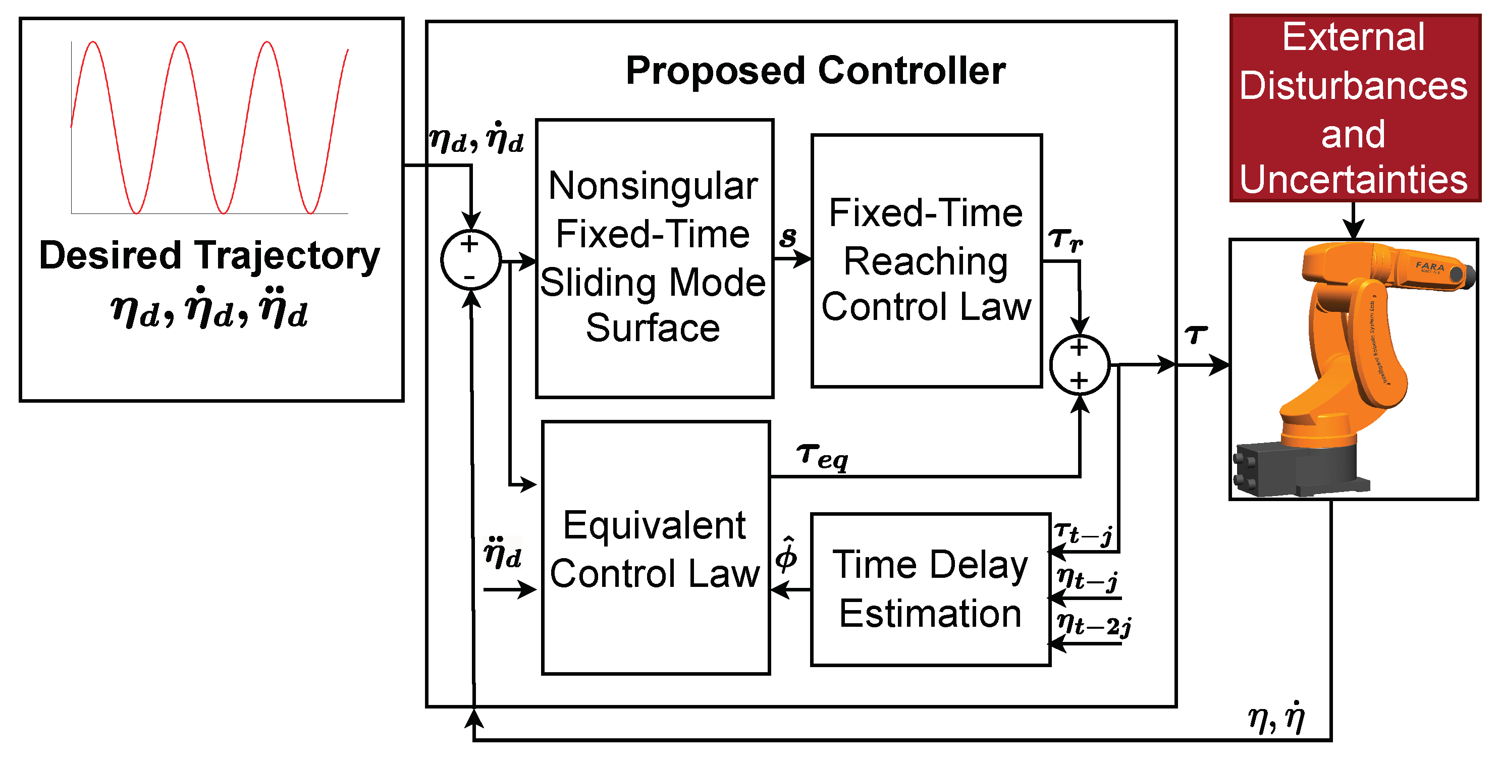
• A MF-NFxTSMC method is introduced, leveraging a TDE mechanism for real-time estimation of unknown dynamics and disturbances. The novelty lies in seamlessly integrating TDE into the nonsingular fixed-time SMC framework with the newly designed SF-FxTSS and FxTRL, enabling robust, model-independent control.
• The fixed-time stability of the closed-loop system is rigorously established using Lyapunov-based analysis, ensuring that convergence time is strictly bounded and independent of initial conditions.
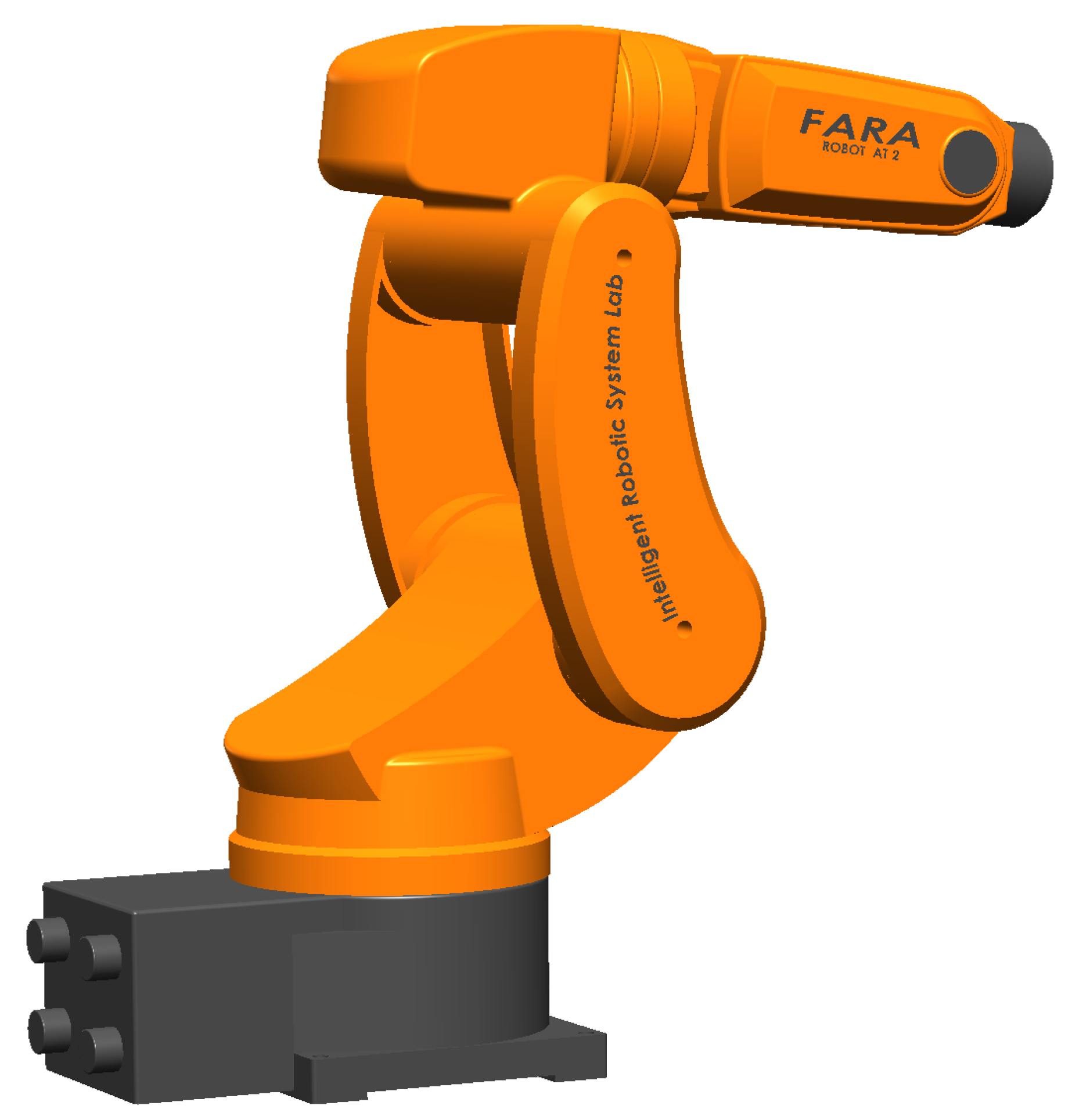
• Extensive simulations on a three-DOF SAMSUNG FARA AT2 robotic manipulator validate the effectiveness of the proposed method. The results demonstrate superior performance in terms of tracking accuracy, convergence speed, and control smoothness compared to conventional SMC, finite-time SMC, approximate fixed-time SMC, and global fixed-time NTSMC methods.

Distinguishing Features: Compared to conventional SMC methods, the proposed MF-NFxTSMC offers the following:

• Model-free operation through real-time estimation, eliminating reliance on physical parameter identification;
• Fixed-time convergence performance, which outperforms finite-time or asymptotic counterparts by ensuring fast convergence even from large initial errors;
• A nonsingular and smooth control structure that avoids singularities and mitigates chattering;
• Practical applicability to real-world manipulators with scalability to higher DOF systems.

The rest of this paper is organized as follows. Section 2 presents the system model, key notations, and relevant preliminaries. Section 3 describes the proposed control design in detail. Section 4 provides simulation results and comparative analysis. Finally, Section 5 concludes the paper and outlines potential future research directions.

2. System Model and Preliminaries

This section introduces the foundational elements necessary for the development of the proposed control methodology, including mathematical notations, the dynamic model of the robotic manipulator, and essential stability concepts. These components collectively establish the analytical groundwork for the subsequent control system design and stability analysis.

2.1. Mathematical Notations

To ensure clarity and consistency in mathematical expressions, we adopt the following notation conventions: scalars are in regular font, vectors are in bold lowercase, and matrices are in bold uppercase. For a vector $\mathit{x}\in {\mathbb{R}}^n$, the i-th element is $x_i$. The sign function and element-wise power are defined as follows:

$$\mathrm{sign}\left(\mathit{x}\right)={[\mathrm{sign}\left(x_1\right),\dots ,\mathrm{sign}\left(x_n\right)]}^T,{\left[x_i\right]}^a={\left|x_i\right|}^a\mathrm{sign}\left(x_i\right),$$

$${\left[\mathit{x}\right]}^a=\left[\right|x_1{|}^a\mathrm{sign}\left(x_1\right),\dots ,|x_n{|}^a\mathrm{sign}\left(x_n\right){]}^T,{\left[\mathit{x}\right]}^{\mathit{a}}=\left[\right|x_1{|}^{a_1}\mathrm{sign}\left(x_1\right),\dots ,|x_n{{|}^{a_n}\mathrm{sign}\left(x_n\right)]}^T,$$

where $\mathit{a}={[a_1,\dots ,a_n]}^T$. The notation $\mathrm{diag}\left\{\mathit{x}\right\}$ represents a diagonal matrix with elements of $\mathit{x}$, and $\parallel \mathit{x}\parallel$ denotes the Euclidean norm.

2.2. Robotic Arm System Description

The dynamic model of an n-joint robotic manipulator can be described by the following nonlinear differential equation:

$$\mathit{H}\left(\mathit{\eta }\right)\ddot{\mathit{\eta }}+\mathit{V}(\mathit{\eta },\dot{\mathit{\eta }})\dot{\mathit{\eta }}+\mathit{g}\left(\mathit{\eta }\right)+\mathit{f}\left(\dot{\mathit{\eta }}\right)=\mathit{\tau }+\mathit{d},$$

(1)

where $\ddot{\mathit{\eta }}\in {\mathbb{R}}^n$ is the vector of joint accelerations, $\dot{\mathit{\eta }}\in {\mathbb{R}}^n$ is the vector of joint velocities, and $\mathit{\eta }\in {\mathbb{R}}^n$ is the vector of joint positions. The matrix $\mathit{H}\left(\mathit{\eta }\right)\in {\mathbb{R}}^{n\times n}$ is the symmetric positive definite inertia matrix, $\mathit{V}(\mathit{\eta },\dot{\mathit{\eta }})\in {\mathbb{R}}^{n\times n}$ denotes the matrix of Coriolis and centrifugal forces, and $\mathit{g}\left(\mathit{\eta }\right)\in {\mathbb{R}}^n$ is the gravity vector. The term $\mathit{f}\left(\dot{\mathit{\eta }}\right)\in {\mathbb{R}}^n$ represents friction forces, $\mathit{\tau }\in {\mathbb{R}}^n$ is the control input (joint torques), and $\mathit{d}\in {\mathbb{R}}^n$ accounts for external disturbances.

For the purpose of control design, Equation (1) is restructured into a more tractable form:

$$\overline{\mathit{H}}\ddot{\mathit{\eta }}+\mathit{\varphi }=\mathit{\tau },$$

(2)

where $\overline{\mathit{H}}$ is a user-defined positive definite diagonal matrix and the lumped term $\mathit{\varphi }\in {\mathbb{R}}^n$ captures all the dynamic components and uncertainties:

$$\mathit{\varphi }=(\mathit{H}\left(\mathit{\eta }\right)-\overline{\mathit{H}})\ddot{\mathit{\eta }}+\mathit{V}(\mathit{\eta },\dot{\mathit{\eta }})\dot{\mathit{\eta }}+\mathit{g}\left(\mathit{\eta }\right)+\mathit{f}\left(\dot{\mathit{\eta }}\right)-\mathit{d}.$$

(3)

2.3. Preliminaries

To support the stability analysis of the proposed control approach, we introduce key definitions and lemmas.

Consider a general nonlinear system:

$$\dot{\mathit{r}}=\xi (\mathit{r},t),\mathit{r}\left(0\right)={\mathit{r}}_0,$$

(4)

where $\mathit{r}\in {\mathbb{R}}^n$ denotes the state vector with an initial value of ${\mathit{r}}_0$, and $\xi (\mathit{r},t):{\mathbb{R}}^n\times {\mathbb{R}}_{\ge 0}\to {\mathbb{R}}^n$ represents a potentially discontinuous vector field. It is assumed that the equilibrium of system (6) is at the origin.

Definition 1 

(Fixed-time stability). The system described by (4) is said to be fixed-time stable if it is globally finite-time stable and the corresponding settling-time function $T\left({\mathit{r}}_0\right)$ is uniformly bounded. That is, there exists a constant $T_{max}>0$ such that $T\left({\mathit{r}}_0\right)\le T_{max}$ for all initial conditions ${\mathit{r}}_0\in {\mathbb{R}}^n$.

Lemma 1 

([32]). Consider the scalar system:

$$\dot{r}=-q_1{\left[r\right]}^{w_1}-q_2{\left[r\right]}^{w_2},$$

(5)

where $q_1>0$, $q_2>0$, $w_1>1$, and $0<w_2<1$. The equilibrium of this system is fixed-time stable, and the settling time is bounded by the following:

$$T_{max}^{L1}\le {\displaystyle \frac{1}{q_1(w_1-1)}}+{\displaystyle \frac{1}{q_2(1-w_2)}}.$$

(6)

Lemma 2 

([33]). Consider the scalar system:

$$\dot{r}=-q_1{\left[r\right]}^{m_1}-q_2{\left[r\right]}^{m_2},$$

(7)

where $q_1>0$, $q_2>0$, $m_1=w_1^{\mathrm{sign}\left(\right|r|-1)}$, $w_1>1$, $m_2=w_2^{\mathrm{sign}(1-|r\left|\right)}$, and $0<w_2<1$. This system is fixed-time stable, with the maximum settling time bounded by the following:

$$T_{max}^{L2}\le {\displaystyle \frac{ln(1+\frac{q_2}{q_1})}{q_2(w_1-1)}}+{\displaystyle \frac{ln(1+\frac{q_1}{q_2})}{q_1(1-w_2)}}.$$

(8)

Remark 1. 

In Lemma 1, the proportionality and exponential coefficients remain fixed, each playing a distinct role in ensuring convergence. Specifically, when the state $\left|r\right|$ is far from the equilibrium ($\left|r\right|\ge 1$), the first term dominates, accelerating the system’s convergence. When the state $\left|r\right|$ is near the equilibrium ($\left|r\right|<1$), the second term takes precedence, ensuring continued convergence. On the other hand, in Lemma 2, the exponential coefficients vary dynamically depending on the state r. This adaptability ensures that both components contribute significantly to the convergence process throughout the trajectory. Consequently, the system in Lemma 2 achieves a faster convergence rate compared to the system in Lemma 1.

3. Design of the Proposed Control Method

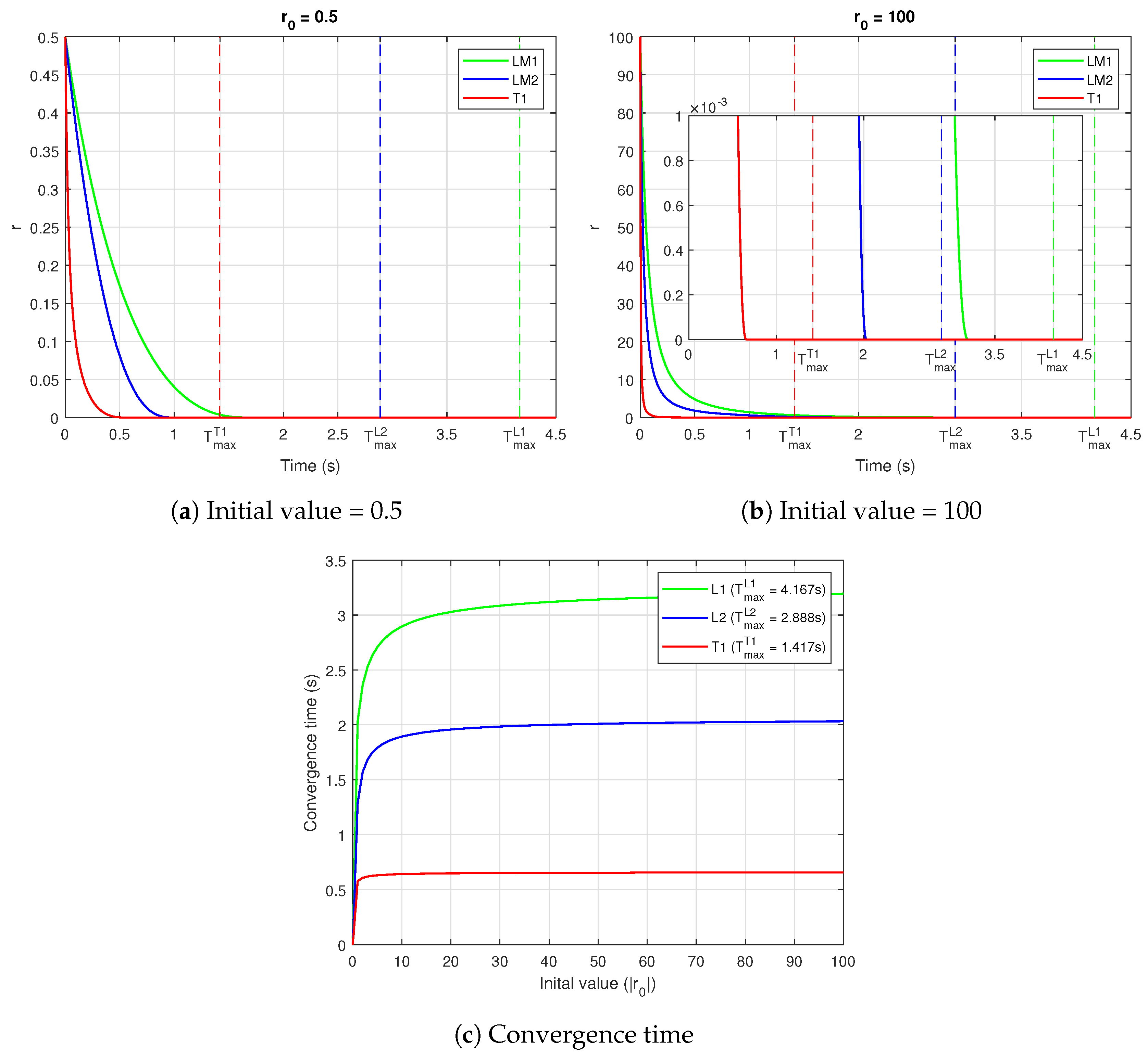
3.1. Novel Fixed-Time Control System

Theorem 1. 

Consider the following dynamical system:

$$\dot{r}=-{\displaystyle \frac{2q}{y\left(r\right)}}{\left[r\right]}^m,$$

(9)

where $y\left(r\right)$ is defined as follows:

$$y\left(r\right)=\sigma +(1-\sigma )\exp (-\gamma |r\left|\right),$$

(10)

with parameters satisfying $0<\sigma <1$, $\gamma \ge 1$, $q>0$, and $m=w^{\mathrm{sign}\left(\right|r|-1)}$, where $w>1$. Under these conditions, the system (9) ensures fixed-time stability, with the upper bound of the settling time given by the following:

$$T_{max}^{T1}\le {\displaystyle \frac{\overline{\sigma }+w}{2q(w-1)}},$$

(11)

where $\overline{\sigma }=\sigma +(1-\sigma )\exp (-\gamma )$.

Proof of Theorem 1.

The proof is established by considering two distinct cases: $\left|r\right|\ge 1$ and $\left|r\right|<1$.

Case 1: $\left|r\right|\ge 1$

For this case, we have $m=w>1$; thus, Equation (9) can be rewritten as follows:

$$\dot{r}=-{\displaystyle \frac{2q}{y\left(r\right)}}{\left[r\right]}^w.$$

(12)

Defining a transformation $x={\left|r\right|}^{1-w}$ and substituting it into Equation (12) yields the following:

$$\begin{array}{cc}\hfill \dot{x}& ={(1-w)\left|r\right|}^{-w}\dot{r}\mathrm{sign}\left(r\right)\hfill \\ \hfill & =-{(1-w)\left|r\right|}^{-w}{\displaystyle \frac{2q}{y\left(r\right)}}{\left|r\right|}^w\hfill \\ \hfill & =-(1-w){\displaystyle \frac{2q}{y\left(r\right)}}.\hfill \end{array}$$

(13)

Observing that $x\in (0,1]$ for $\left|r\right|\in [1,\infty )$, the settling time can be derived by integrating Equation (13):

$$\begin{array}{cc}\hfill {\int }_0^{T_1}dt& =-{\int }_0^1{\displaystyle \frac{y\left(r\right)}{2q(1-w)}}dx={\int }_0^1{\displaystyle \frac{y\left(r\right)}{2q(w-1)}}dx.\hfill \end{array}$$

(14)

Since $\sigma \le y\left(r\right)\le \overline{\sigma }$ for $\left|r\right|\in [1,\infty )$, Equation (14) can be bounded as follows:

$$\begin{array}{cc}\hfill T_1& \le {\int }_0^1{\displaystyle \frac{\overline{\sigma }}{2q(w-1)}}dx\hfill \\ \hfill & \le {\displaystyle \frac{\overline{\sigma }}{2q(w-1)}}.\hfill \end{array}$$

(15)

Case 2: $\left|r\right|<1$

For this case, we set $m=1/w<1$, and Equation (9) can be reformulated as follows:

$$\dot{r}=-{\displaystyle \frac{2q}{y\left(r\right)}}{\left[r\right]}^{{\displaystyle \frac{1}{w}}}.$$

(16)

Introducing the transformation $h={\left|r\right|}^{1-{\displaystyle \frac{1}{w}}}$ and substituting it into Equation (16), we obtain the following:

$$\begin{array}{cc}\hfill \dot{h}& =\left(1-{\displaystyle \frac{1}{w}}\right){\left|r\right|}^{-{\displaystyle \frac{1}{w}}}\dot{r}\mathrm{sign}\left(r\right)\hfill \\ \hfill & =-\left(1-{\displaystyle \frac{1}{w}}\right){\left|r\right|}^{-{\displaystyle \frac{1}{w}}}{\displaystyle \frac{2q}{y\left(r\right)}}{\left|r\right|}^{{\displaystyle \frac{1}{w}}}\hfill \\ \hfill & =-{\displaystyle \frac{w-1}{w}}{\displaystyle \frac{2q}{y\left(r\right)}}.\hfill \end{array}$$

(17)

Noting that $h\in [0,1)$ for $\left|r\right|\in [0,1)$, the settling time can be computed by integrating Equation (17):

$${\int }_0^{T_2}dt=-{\int }_1^0{\displaystyle \frac{wy\left(r\right)}{2q(w-1)}}dh={\int }_0^1{\displaystyle \frac{wy\left(r\right)}{2q(w-1)}}dh.$$

(18)

Given that $\overline{\sigma }\le y\left(r\right)\le 1$ for $\left|r\right|\in [0,1)$, we can bound Equation (18) as follows:

$$\begin{array}{cc}\hfill T_2& \le {\int }_0^1{\displaystyle \frac{w}{2q(w-1)}}dh\hfill \\ \hfill & \le {\displaystyle \frac{w}{2q(w-1)}}.\hfill \end{array}$$

(19)

Finally, from Equations (15) and (19), the total settling time is obtained as follows:

$$\begin{array}{cc}\hfill T_{max}^{T1}& \le T_1+T_2\hfill \\ \hfill & \le {\displaystyle \frac{\overline{\sigma }+w}{2q(w-1)}}.\hfill \end{array}$$

(20)

Since the settling time is uniformly bounded and does not depend on the initial state, the system (9) is globally fixed-time stable within time $T_{max}^{T1}$.

This concludes the proof. □

Remark 2. 

Theorem 1 not only inherits the advantages of Lemma 2 but also significantly enhances its convergence properties. Specifically, the proposed system introduces the dynamically varying coefficients $y\left(r\right)$ and w, where $y\left(r\right)$ fine-tunes the proportional factor, and w adapts the exponential factor based on the system state. In Lemma 2, the self-adaptive exponential terms ensure that both components contribute equally to each stage of convergence. Building on this concept, the proposed system employs only one self-adaptive mechanism that preserves simplicity while maintaining robustness.

A key distinction of Theorem 1 is its adaptive nature, which contrasts with conventional fixed-time systems that rely on constant parameters. The function $y\left(r\right)$ dynamically adjusts the control gain, ensuring that when $\left|r\right|$ is large (i.e., the system is far from equilibrium), the control effort remains high to accelerate convergence. As $\left|r\right|$ approaches zero, $y\left(r\right)$ gradually decreases, preventing excessive overshoot while maintaining fast convergence. This adaptive scaling mechanism optimally balances convergence speed and stability, making the system more resilient to variations in initial conditions. Thus, Theorem 1 provides a superior control strategy with a fast convergence rate, leading to a more efficient fixed-time stabilization compared to Lemmas 1 and 2.

Remark 3. 

To illustrate the convergence behavior of fixed-time stable systems, we conducted simulations comparing the performance of the systems in Lemma 1, Lemma 2, and Theorem 1, denoted as L1, L2, and T1, respectively. The system parameters were set as follows: $m_1=m_2=m=1$, $w_1=w=1.6$, $w_2=0.6$, $\sigma =0.1$, and $\gamma =10$. Based on these parameters, the theoretical upper bounds of the settling times were determined as $T_{max}^{L1}<4.167$ s, $T_{max}^{L2}<2.888$ s, and $T_{max}^{T1}<1.417$ s. Figure 1a,b presents the convergence characteristics of the three methods under different initial conditions. The results confirm that all systems converge before their respective theoretical settling times, validating the property of the fixed-time stability. As shown in Figure 1c, L2 exhibits a faster convergence rate compared to L1, demonstrating the benefit of introducing self-adaptive exponentiation. More importantly, the proposed method (T1) significantly outperforms both L1 and L2, achieving the fastest convergence across different initial conditions. A key advantage of this proposed system is its ability to accelerate convergence, whether it is far from equilibrium or very close to it. This capability ensures rapid stabilization and improved robustness.

3.2. Novel Nonsingular Fixed-Time Sliding Mode Surface

To achieve precise trajectory tracking, we define the position and velocity tracking errors as follows:

$$\mathit{e}={\mathit{\eta }}_{\mathit{d}}-\mathit{\eta },\dot{\mathit{e}}={\dot{\mathit{\eta }}}_{\mathit{d}}-\dot{\mathit{\eta }},$$

(21)

where ${\mathit{\eta }}_{\mathit{d}}$ and ${\dot{\mathit{\eta }}}_{\mathit{d}}$ represent the desired position and velocity trajectories, respectively.

Building upon the fixed-time stabilization framework established in Theorem 1, we propose a novel SF-FxTSS formulated as follows:

$$s_i={\dot{e}}_i+{\displaystyle \frac{2a_i}{z_i\left(e_i\right)}}{\kappa }_i\left(e_i\right),i=1,\dots ,n,$$

(22)

where ${\kappa }_i\left(e_i\right)$ and $z_i\left(e_i\right)$ are defined as follows:

$${\kappa }_i\left(e_i\right)=\left\{\begin{array}{cc}{e}_i,\hfill & \mathrm{if}{e}_i=0,\hfill \\ [e_i{]}^{p_i},\hfill & \mathrm{otherwise},\hfill \end{array}\right.$$

(23)

$$z_i\left(e_i\right)={\vartheta }_i+(1-{\vartheta }_i)\exp (-{\varsigma }_i|e_i\left|\right),$$

(24)

with parameters satisfying $0<{\vartheta }_i<1$, ${\varsigma }_i\ge 1$, and $a_i>0$. The exponent $p_i$ is defined as $p_i={\alpha }_i^{\mathrm{sign}\left(\right|e_i|-1)}$, where $1<{\alpha }_i<2$.

Remark 4. 

The proposed sliding surface in Equation (22) incorporates key properties of the fixed-time stabilization framework from Theorem 1. Specifically, by incorporating the proportional term $z_i\left(e_i\right)$ and the adaptive exponent $p_i$, the design enables dynamic adjustment of the convergence rate while ensuring that the tracking error converges to zero within a fixed time, independent of the initial condition.

A distinctive and important feature of this design is the smooth and well-defined transition between the nonlinear and linear regimes at $e_i=0$, as clarified in Equation (23). In conventional terminal or fixed-time sliding mode surfaces, singularities often arise when $e_i=0$ and ${\dot{e}}_i\ne 0$, primarily due to the presence of fractional exponent terms such as $|e_i{|}^w$ with $0<w<1$. These terms become unbounded in their derivatives at the origin, which can destabilize the system or lead to control discontinuities. The proposed sliding surface explicitly avoids this issue by defining a nonsingular behavior at the origin using a piecewise function, thereby ensuring continuous and robust performance across the entire state space. Furthermore, in contrast to recently proposed fixed-time sliding surfaces [34,35,36] that utilize boundary layer techniques to switch between sliding regimes, thereby increasing control complexity and leading only to convergence within a bounded region, the proposed sliding surface guarantees global fixed-time convergence to the exact equilibrium point without introducing additional control layers or approximations.

This design not only simplifies the control implementation but also enhances the robustness and precision of the system, making it particularly suitable for practical applications where strict tracking and robustness requirements are essential.

Theorem 2. 

Consider the system governed by the tracking error dynamics in (21). Once the tracking errors reach the sliding surface (22), i.e., $s_i=0$, they will converge to zero within a fixed time, independent of the initial conditions. Specifically, the upper bound of the settling time is given by the following:

$$T_{si}\le {\displaystyle \frac{{\overline{\vartheta }}_i+{\alpha }_i}{2a_i({\alpha }_i-1)}},$$

(25)

where ${\overline{\vartheta }}_i={\vartheta }_i+(1-{\vartheta }_i)\exp (-{\varsigma }_i)$.

Proof of Theorem 2.

Once the system trajectories reach the sliding surface (22), the sliding condition $s_i=0$ holds. From (22), the tracking error dynamics satisfy the following:

$${\dot{e}}_i=-{\displaystyle \frac{2a_i}{z_i\left(e_i\right)}}{\kappa }_i\left(e_i\right).$$

(26)

For $e_i\ne 0$, substituting (23) into (26) yields the following:

$${\dot{e}}_i=-{\displaystyle \frac{2a_i}{z_i\left(e_i\right)}}{\left[e_i\right]}^{p_i}.$$

(27)

Equation (27) follows the fixed-time stability form presented in Theorem 1. Consequently, the tracking errors $e_i$ converge to zero within a fixed time, bounded by the following:

$$T_{si}\le {\displaystyle \frac{{\overline{\vartheta }}_i+{\alpha }_i}{2a_i({\alpha }_i-1)}}.$$

(28)

Thus, the fixed-time convergence of the tracking errors is established, completing the proof. □

Taking the time derivative of the sliding mode surface (22), we obtain the following:

$$\begin{array}{cc}\hfill \dot{\mathit{s}}& ={\ddot{\mathit{\eta }}}_d-\ddot{\mathit{\eta }}+\mathit{\psi },\hfill \end{array}$$

(29)

where $\mathit{\psi }={[{\psi }_1,\dots ,{\psi }_n]}^T$ is defined as follows:

$${\psi }_i={\displaystyle \frac{2a_i}{z_i^2}}({\dot{\kappa }}_i{z}_i-{\kappa }_i{\dot{z}}_i),$$

(30)

with ${\dot{z}}_i=-{\varsigma }_i(1-{\vartheta }_i)\exp (-{\varsigma }_i|e_i\left|\right)\mathrm{sign}\left(e_i\right){\dot{e}}_i$, and ${\dot{\kappa }}_i$ is given by the following:

$${\dot{\kappa }}_i=\left\{\begin{array}{cc}{\dot{e}}_i,\hfill & \mathrm{if}{e}_i=0,\hfill \\ p_i{\left|e_i\right|}^{p_i-1}{\dot{e}}_i,\hfill & \mathrm{otherwise}.\hfill \end{array}\right.$$

(31)

Substituting the system dynamics from Equation (2) into Equation (29), we obtain the following:

$$\begin{array}{c}\hfill \dot{\mathit{s}}={\ddot{\mathit{\eta }}}_d-{\overline{\mathit{H}}}^{-1}(\mathit{\tau }-\mathit{\varphi })+\mathit{\psi }.\end{array}$$

(32)

Accurate modeling of the system dynamics and mitigating the adverse effects of external disturbances pose significant challenges in control design. To address these issues, this study leverages the TDE technique to approximate the entire dynamic model and associated uncertainties, thereby enabling a model-free control approach.

Using Equation (2), the estimated value of $\mathit{\varphi }$ based on the TDE technique [37] is given by the following:

$$\widehat{\mathit{\varphi }}={\mathit{\tau }}_{t-j}-\overline{\mathit{H}}{\ddot{\mathit{\eta }}}_{t-j},$$

(33)

where ${•}_{t-j}$ represents the time-delayed value of ${•}_t$, and j is the time-delay constant, typically selected as the sampling time. The time-delayed acceleration ${\dot{\mathit{\eta }}}_{t-j}$ is computed as follows:

$${\ddot{\mathit{\eta }}}_{t-j}=\left\{\begin{array}{cc}0,\hfill & \mathrm{if}t\le P,\hfill \\ {\displaystyle \frac{{\mathit{\eta }}_t-2{\mathit{\eta }}_{t-j}+{\mathit{\eta }}_{t-2j}}{j^2}},\hfill & \mathrm{if}t>P,\hfill \end{array}\right.$$

(34)

where P can be set as $P\ge 2j$ to effectively reduce significant fluctuations in the initial phase of ${\dot{\mathit{\eta }}}_{t-j}$. Still, it must not be overly large to ensure accuracy.

By incorporating this estimation, Equation (32) can be rewritten as follows:

$$\dot{\mathit{s}}={\ddot{\mathit{\eta }}}_d-{\overline{\mathit{H}}}^{-1}(\mathit{\tau }-\widehat{\mathit{\varphi }})+\tilde{\mathit{\varphi }}+\mathit{\psi },$$

(35)

where $\tilde{\mathit{\varphi }}={\overline{\mathit{H}}}^{-1}(\mathit{\varphi }-\widehat{\mathit{\varphi }})$ represents the TDE error.

Remark 5. 

The selection of $\overline{\mathit{H}}$ plays a crucial role in ensuring the accuracy of TDE. If $\overline{M}$ is properly tuned to satisfy $\parallel \mathit{I}-{\mathit{H}}^{-1}\overline{\mathit{H}}\parallel <1$ and the delay constant is chosen sufficiently small (i.e., $j\to 0$), then the TDE error remains bounded, such that $\parallel \tilde{\mathit{\varphi }}\parallel <\overline{\mathit{\varphi }}$, where $\overline{\mathit{\varphi }}>0$ [37]. This result, as confirmed in [37], guarantees that the TDE method effectively approximates the system dynamics and compensates for uncertainties. By leveraging this estimated information, a model-free control strategy can be established, eliminating the dependency on explicit system modeling while maintaining robust performance in uncertain environments.

3.3. Novel Model-Free Nonsingular Fixed-Time Sliding Mode Control

Building upon Equation (35), a novel MF-NFxTSMC law is formulated as follows:

$$\mathit{\tau }={\mathit{\tau }}_{eq}+{\mathit{\tau }}_r,$$

(36)

$${\mathit{\tau }}_{eq}=\widehat{\mathit{\varphi }}+\overline{\mathit{H}}\left({\ddot{\mathit{\eta }}}_d+\mathit{\psi }\right),$$

(37)

$${\mathit{\tau }}_r=\overline{\mathit{H}}\left(\overline{\varphi }\mathrm{sign}\left(\mathit{s}\right)+\mathit{K}{\left[\mathit{s}\right]}^{\omega }\right),$$

(38)

where ${\mathit{\tau }}_{eq}$ represents the equivalent control law, and ${\mathit{\tau }}_r$ denotes the novel fixed-time reaching control law developed based on Theorem 1. The gain matrix is defined as $\mathit{K}=\mathrm{diag}\left\{{\displaystyle \frac{2b_i}{{\delta }_i\left(s_i\right)}}\right\}$, with ${\delta }_i\left(s_i\right)={\mu }_i+(1-{\mu }_i)exp(-{\epsilon }_i|s_i\left|\right)$. The parameters satisfy $b_i>0$, $0<{\mu }_i<1$, and ${\epsilon }_i\ge 1$, and the adaptive exponent $\mathit{\omega }={[{\omega }_1,...,{\omega }_n]}^T$ is given by ${\omega }_i={\lambda }_i^{\mathrm{sign}\left(\right|s_i|-1)}$, where ${\lambda }_i>1$ for $i=1,...,n$.

The proposed control scheme is illustrated in the block diagram shown in Figure 2, highlighting the integration of the model-free fixed-time control strategy.

Theorem 3. 

Given the SF-FxTSS defined in Equation (22) and the control law designed in Equations (36)–(38), the closed-loop system governing the robotic manipulator (2) is globally fixed-time stable.

Proof of Theorem 3.

Substituting the control law from Equations (36)–(38) into Equation (35), we obtain the following:

$$\dot{\mathit{s}}=\tilde{\mathit{\varphi }}-\overline{\varphi }\mathrm{sign}\left(\mathit{s}\right)-\mathit{K}{\left[\mathit{s}\right]}^{\omega }.$$

(39)

To analyze stability, consider the Lyapunov function candidate:

$$V_{ri}=s_i^2.$$

(40)

Differentiating Equation (40) with respect to time yields the following:

$$\begin{array}{cc}\hfill {\dot{V}}_{ri}& =2s_i\left({\tilde{\varphi }}_i-\overline{\varphi }\mathrm{sign}\left(s_i\right)-{\displaystyle \frac{2b_i}{{\delta }_i\left(s_i\right)}}{\left[s_i\right]}^{{\omega }_i}\right),\hfill \\ \hfill & \le 2|s_i|({\tilde{\varphi }}_i-\overline{\varphi })-{\displaystyle \frac{4b_i}{{\delta }_i\left(s_i\right)}}{\left|s_i\right|}^{{\omega }_i+1},\hfill \\ \hfill & \le -{\displaystyle \frac{4b_i}{{\delta }_i(V_{ri}^{\frac{1}{2}})}}{V}_{ri}^{{\displaystyle \frac{{\omega }_i+1}{2}}}<0.\hfill \end{array}$$

(41)

Since $V_{ri}>0$ and ${\dot{V}}_{ri}<0$, the sliding surface is ensured to converge to zero. The exact settling time can be determined by integrating Equation (41):

$$\underset{0}{\overset{T_{ri}}{\int }}dt=\underset{1}{\overset{\infty }{\int }}{\displaystyle \frac{{\delta }_i(V_{ri}^{\frac{1}{2}})}{4b_i{V}_{ri}^{\frac{{\omega }_i+1}{2}}}}d{V}_{ri}+\underset{0}{\overset{1}{\int }}{\displaystyle \frac{{\delta }_i(V_{ri}^{\frac{1}{2}})}{4b_i{V}_{ri}^{\frac{{\omega }_i+1}{2}}}}d{V}_{ri}.$$

(42)

Using the bounds ${\mu }_i\le {\delta }_i(V_{ri}^{{\displaystyle \frac{1}{2}}})\le {\overline{\mu }}_i={\mu }_i+(1-{\mu }_i)exp(-{\epsilon }_i)$ for $V_i\in [1,\infty )$, and ${\overline{\mu }}_i\le {\delta }_i(V_{ri}^{{\displaystyle \frac{1}{2}}})\le 1$ for $V_i\in [0,1)$, we obtain the following:

$$\begin{array}{cc}\hfill T_{ri}& \le \underset{1}{\overset{\infty }{\int }}{\displaystyle \frac{{\overline{\mu }}_i}{4b_i{V}_{ri}^{\frac{{\lambda }_i+1}{2}}}}d{V}_{ri}+\underset{0}{\overset{1}{\int }}{\displaystyle \frac{1}{4b_i{V}_{ri}^{\frac{1/{\lambda }_i+1}{2}}}}d{V}_{ri},\hfill \\ \hfill & \le {\displaystyle \frac{{\overline{\mu }}_i}{2b_i({\lambda }_i-1)}}+{\displaystyle \frac{{\lambda }_i}{2b_i({\lambda }_i-1)}},\hfill \\ \hfill & \le {\displaystyle \frac{{\overline{\mu }}_i+{\lambda }_i}{2b_i({\lambda }_i-1)}}.\hfill \end{array}$$

(43)

From Equation (43), it follows that the sliding mode surface reaches zero within a fixed time, with an upper bound on the settling time given by $T_{ri}$. This completes the proof. □

By combining Theorems 2 and 3, the total convergence time for the tracking error to reach zero can be computed as $T_{ci}=T_{si}+T_{ri}$. Consequently, the maximum guaranteed convergence time of the system satisfies the following:

$$T_{max}<\underset{i=1,\dots ,n}{max}{T}_{ci}.$$

(44)

This confirms that the proposed MF-NFxTSMC law ensures fixed-time convergence of tracking errors, providing strong robustness and enhanced control performance in uncertain environments.

4. Simulation Setup and Performance Evaluation

4.1. Simulation Environment and System Configuration

To assess the effectiveness of the proposed control strategy, comprehensive numerical simulations were carried out using the MATLAB/Simulink2021b environment. The simulation model is based on a three-DOF SAMSUNG FARA AT2 robotic manipulator.

A detailed 3D CAD model of the robotic arm was developed using SolidWorks2018, as depicted in Figure 3, and subsequently integrated into Simulink through the Simscape Multibody Link tool. This modeling technique allows the simulation setup to accurately represent the real-world dynamics and kinematics of the physical system, thereby enhancing the credibility of the findings.

All simulations were conducted with a fixed sampling time of 0.001 s to guarantee high-resolution time-domain behavior and stable numerical integration. The mechanical properties and dynamic parameters of the robot, including mass, inertia, and joint configuration, are elaborated in our prior work [38].

4.2. Control Methods for Comparison

To validate the superiority of the proposed control approach (denoted as A5), it is benchmarked against four well-established control strategies:

• A1: Conventional SMC.
• A2: Finite-time SMC [39].
• A3: Approximate fixed-time SMC [34].
• A4: Global fixed-time NTSMC [36].

The corresponding control laws for these comparative methods are detailed below:

Method A1: 

$$\begin{array}{cc}\hfill \mathit{s}& =\dot{\mathit{e}}+{\mathit{C}}_0\mathit{e},\hfill \end{array}$$

(45)

$$\begin{array}{cc}\hfill \mathit{\tau }& =\widehat{\mathit{H}}\left(\mathit{\eta }\right)\left({\ddot{\mathit{\eta }}}_d+{\mathit{C}}_0\dot{\mathit{e}}+{\mathit{M}}_0\mathrm{sign}\left(\mathit{s}\right)+{\mathit{M}}_1\mathit{s}\right)+\widehat{\mathit{V}}(\mathit{\eta },\dot{\mathit{\eta }})\dot{\mathit{\eta }}+\widehat{\mathit{g}}\left(\mathit{\eta }\right),\hfill \end{array}$$

(46)

where ${\mathit{C}}_0$, ${\mathit{M}}_0$, and ${\mathit{M}}_1$ are positive diagonal matrices.

Method A2: 

$$\begin{array}{cc}\hfill \mathit{s}& =\mathit{e}+{\mathit{C}}_1{\left[\mathit{e}\right]}^{{\theta }_1}+{\mathit{C}}_2{\left[\dot{\mathit{e}}\right]}^{{\theta }_2},\hfill \end{array}$$

(47)

$$\begin{array}{cc}\hfill \mathit{\tau }& =\widehat{\mathit{H}}\left(\mathit{\eta }\right)\left({\ddot{\mathit{\eta }}}_d+{\mathit{\phi }}_2+{\mathit{M}}_0\mathrm{sign}\left(\mathit{s}\right)+{\mathit{M}}_1\mathit{s}\right)+\widehat{\mathit{V}}(\mathit{\eta },\dot{\mathit{\eta }})\dot{\mathit{\eta }}+\widehat{\mathit{g}}\left(\mathit{\eta }\right),\hfill \end{array}$$

(48)

where ${\mathit{\phi }}_2={[{\phi }_{21},...,{\phi }_{2n}]}^T$ with

$${\phi }_{2i}={\displaystyle \frac{\left(1+C_{1i}{\theta }_{1i}{\left|e_i\right|}^{{\theta }_{1i}-1}\right){\left|{\dot{e}}_i\right|}^{2-{\theta }_{2i}}\mathrm{sign}\left({\dot{e}}_i\right)}{C_{2i}{\theta }_{2i}}},$$

${\mathit{\theta }}_1={[{\theta }_{11},...,{\theta }_{1n}]}^T$, ${\mathit{\theta }}_2={[{\theta }_{21},...,{\theta }_{2n}]}^T$, where ${\theta }_{1i}>{\theta }_{2i}$, $1<{\theta }_{2i}<2$, and ${\mathit{M}}_0,{\mathit{M}}_1$ are as defined in A1.

Method A3: 

$$\begin{array}{cc}\hfill s_i& ={\dot{e}}_i+C_{3i}{v}^{{\theta }_{3i}}\left(e_i\right)+C_{4i}{\left[e_i\right]}^{{\theta }_{4i}},\hfill \end{array}$$

(49)

$$\begin{array}{cc}\hfill v^{{\theta }_{3i}}\left(e_i\right)& =\left\{\begin{array}{cc}{\left[e_i\right]}^{{\theta }_{3i}},\hfill & \mathrm{if}|e_i|\ge \zeta ,\hfill \\ {\zeta }^{{\theta }_{3i}-1}{e}_i,\hfill & \mathrm{otherwise}\hfill \end{array}\right.,{\dot{v}}^{{\theta }_{3i}}\left(e_i\right)=\left\{\begin{array}{cc}{\theta }_{3i}{\left|e_i\right|}^{{\theta }_{3i}-1}{\dot{e}}_i,\hfill & \mathrm{if}|e_i|\ge \zeta ,\hfill \\ {\zeta }^{{\theta }_{3i}-1}{\dot{e}}_i,\hfill & \mathrm{otherwise}\hfill \end{array}\right.,\hfill \end{array}$$

(50)

$$\begin{array}{cc}\hfill \mathit{\tau }& =\widehat{\mathit{H}}\left(\mathit{\eta }\right)\left({\ddot{\mathit{\eta }}}_d+{\phi }_3+{\mathit{M}}_0\mathrm{sign}\left(\mathit{s}\right)+{\mathit{M}}_2{\left[\mathit{s}\right]}^{{\chi }_2}\right)+\widehat{\mathit{V}}(\mathit{\eta },\dot{\mathit{\eta }})\dot{\mathit{\eta }}+\widehat{\mathit{g}}\left(\mathit{\eta }\right),\hfill \end{array}$$

(51)

where ${\mathit{\phi }}_3={[{\phi }_{31},...,{\phi }_{3n}]}^T$ with

$${\phi }_{3i}=C_{3i}{\dot{v}}^{{\theta }_{3i}}\left(e_i\right)+C_{4i}{\theta }_{4i}{\left|e_i\right|}^{{\theta }_{4i}-1}{\dot{e}}_i,$$

$C_{3i},C_{4i}>0$, $0<{\theta }_{3i}<1$, ${\theta }_{4i}>1$, $0<\zeta <1$, and ${\mathit{M}}_2$ is a positive diagonal matrix. Also, ${\mathit{\chi }}_2={[{\chi }_{21},...,{\chi }_{2n}]}^T$ with ${\chi }_{2i}>1$.

Method A4: 

A fixed-time observer is incorporated to estimate the lumped disturbance:

$$\begin{array}{c}\hfill \left\{\begin{array}{c}{\dot{\widehat{\mathit{x}}}}_2=C_8\left({\left[{\displaystyle \frac{\dot{\mathit{\eta }}-{\widehat{\mathit{x}}}_2}{o}}\right]}^{{\theta }_8}+{\left[{\displaystyle \frac{\dot{\mathit{\eta }}-{\widehat{\mathit{x}}}_2}{o}}\right]}^{{\theta }_9}\right)+\widehat{\mathbf{\Xi }}+{\widehat{\mathit{H}}}^{-1}\left(\mathit{\eta }\right)(\mathit{\tau }-\widehat{\mathit{V}}(\mathit{\eta },\dot{\mathit{\eta }})\dot{\mathit{\eta }}-\widehat{\mathit{g}}\left(\mathit{\eta }\right))\hfill \\ \dot{\widehat{\mathbf{\Xi }}}=C_9\left({\left[{\displaystyle \frac{\dot{\mathit{\eta }}-{\widehat{\mathit{x}}}_2}{o}}\right]}^{2{\theta }_8-1}+{\left[{\displaystyle \frac{\dot{\mathit{\eta }}-{\widehat{\mathit{x}}}_2}{o}}\right]}^{2{\theta }_9-1}\right)\hfill \end{array}\right.\end{array}$$

(52)

where $C_8,C_9>0$, $C_8\ge 2\sqrt{C_9}$, $0<{\theta }_8<1$, $1<{\theta }_9<1.5$, and $0<o<1$.

The control law is formulated as follows:

$$\begin{array}{cc}\hfill s_i& ={\dot{e}}_i+C_{5i}{\left[e_i\right]}^{{\theta }_{5i}}+C_{6i}{e}_i+C_{7i}{\varpi }^{{\theta }_{7i}}\left(e_i\right),\hfill \end{array}$$

(53)

$$\begin{array}{cc}\hfill {\varpi }^{{\theta }_{7i}}\left(e_i\right)& =\left\{\begin{array}{cc}{\left[e_i\right]}^{{\theta }_{7i}},\hfill & \mathrm{if}|e_i|\ge l,\hfill \\ {\iota }_{1i}{e}_i+{\iota }_{2i}{\left[e_i\right]}^2+{\iota }_{3i}{e}_i^3,\hfill & \mathrm{otherwise}\hfill \end{array}\right.,\hfill \end{array}$$

(54)

$$\begin{array}{cc}\hfill {\dot{\varpi }}^{{\theta }_{7i}}\left(e_i\right)& =\left\{\begin{array}{cc}{\theta }_{7i}{\left|e_i\right|}^{{\theta }_{7i}-1}{\dot{e}}_i,\hfill & \mathrm{if}|e_i|\ge l,\hfill \\ {\iota }_{1i}{\dot{e}}_i+2{\iota }_{2i}\left|e_i\right|{\dot{e}}_i+3{\iota }_{3i}{e}_i^2{\dot{e}}_i,\hfill & \mathrm{otherwise}\hfill \end{array}\right.,\hfill \end{array}$$

(55)

$$\begin{array}{cc}\hfill \mathit{\tau }& =\widehat{\mathit{H}}\left(\mathit{\eta }\right)\left({\ddot{\mathit{\eta }}}_d+{\phi }_4-\widehat{\mathbf{\Xi }}+{\mathit{M}}_3\mathrm{sign}\left(\mathit{s}\right)+{\mathit{M}}_4{\left[\mathit{s}\right]}^{{\chi }_4}+{\mathit{M}}_5\mathit{s}+{\mathit{M}}_6{\left[\mathit{s}\right]}^{{\chi }_6}\right)\hfill \\ \hfill & +\widehat{\mathit{V}}(\mathit{\eta },\dot{\mathit{\eta }})\dot{\mathit{\eta }}+\widehat{\mathit{g}}\left(\mathit{\eta }\right),\hfill \end{array}$$

(56)

where ${\mathit{\phi }}_4={[{\phi }_{41},...,{\phi }_{4n}]}^T$ with

$${\phi }_{4i}=C_{5i}{\theta }_{5i}{\left|e_i\right|}^{{\theta }_{5i}-1}{\dot{e}}_i+C_{6i}{\dot{e}}_i+C_{7i}{\dot{\varpi }}^{{\theta }_{7i}}\left(e_i\right),$$

and scalar gains satisfy $C_{5i}$, $C_{6i}$, $C_{7i}>0$. Additional parameters include ${\theta }_{5i}>1$, $0.5<{\theta }_{7i}<1$, $0<l<1$, ${\iota }_{1i}=({\theta }_{7i}-2)({\theta }_{7i}-3)l^{{\theta }_{7i}-1}/2$, ${\iota }_{2i}=(1-{\theta }_{7i})({\theta }_{7i}-3)l^{{\theta }_{7i}-2}$, ${\iota }_{3i}=({\theta }_{7i}-1)({\theta }_{7i}-2)l^{{\theta }_{7i}-3}/2$, ${\chi }_4={[{\chi }_{41},...,{\chi }_{4n}]}^T$ with ${\chi }_{4i}>1$, and ${\chi }_6={[{\chi }_{61},...,{\chi }_{6n}]}^T$ with $0<{\chi }_{6i}<1$. The matrices ${\mathit{M}}_3$, ${\mathit{M}}_4$, ${\mathit{M}}_5$, and ${\mathit{M}}_6$ are positive diagonal matrices.

The parameters for all control methods used in the simulations are summarized in

Table 1. Parameters of control methods.

Method	Parameter	Value
A1	$C_{0i}$, $M_{0i}$, $M_{1i}$	6, 10, 6
A2	$C_{1i}$, $C_{2i}$, ${\theta }_{1i}$, ${\theta }_{2i}$, $M_{0i}$, $M_{1i}$	6, 0.8, 1.1, 1.08, 10, 6
A3	$C_{3i}$, $C_{4i}$, ${\theta }_{3i}$, ${\theta }_{4i}$, $\zeta$, $M_{0i}$, $M_{2i}$, ${\chi }_{2i}$	6, 6, $0.8$, $1.1$, $0.002$, 10, 6, $1.1$
A4	$C_{5i}$, $C_{6i}$, $C_{7i}$, ${\theta }_{5i}$, ${\theta }_{7i}$, l, $M_{3i}$, $M_{4i}$, $M_{5i}$, $M_{6i}$, ${\chi }_{4i}$, ${\chi }_{6i}$, $C_8$, $C_9$, ${\theta }_8$, ${\theta }_9$, o	6, 6, 6, $1.1$, $0.8$, $0.002$, $0.05$, 3, 3, 3, $1.1$, $0.8$, $2\sqrt{6}$, 5, $0.8$, $1.2$, $0.01$
A5	$a_i$, ${\vartheta }_i$, ${\varsigma }_i$, ${\alpha }_i$, $\overline{\varphi }$, $b_i$, ${\mu }_i$, ${\epsilon }_i$, ${\lambda }_i$ $\overline{\mathit{H}}$, j, P	6, $0.5$, 6, $1.25$, $0.01$, 6, $0.5$, 6, $1.25$ $\mathrm{diag}\{0.4,0.8,0.2\}$, $0.001$, $0.002$

.

4.3. Simulation Settings

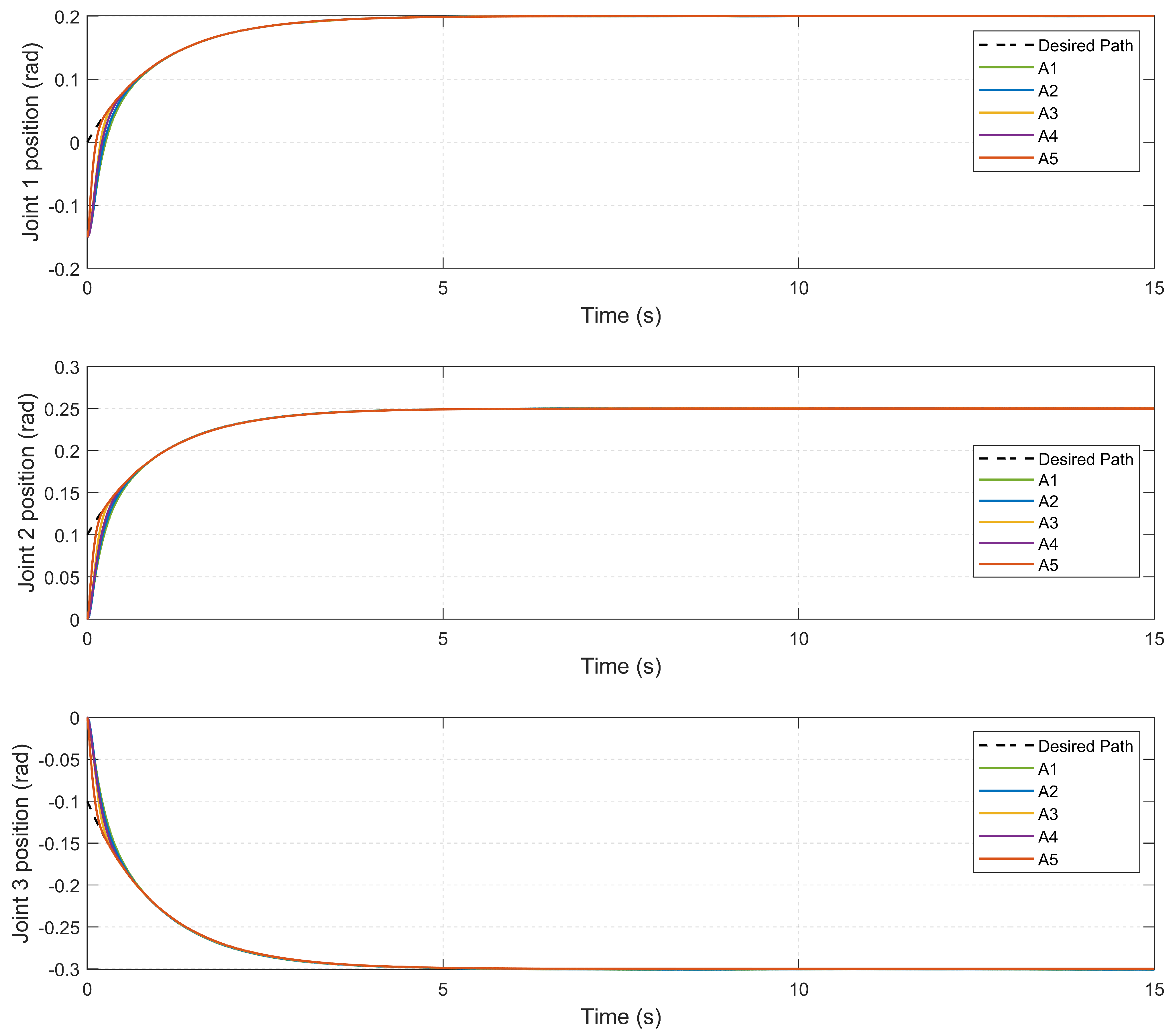
To examine the robustness of each control method, the system is subjected to external disturbances and nonlinear friction effects. The joint disturbances are defined as follows:

$$\mathit{d}\left(t\right)={[2sin\left(t\right)+sin\left(2t\right),-sin\left(t\right)-sin\left(2t\right),0.5sin\left(t\right)-0.5sin\left(2t\right)]}^T,$$

and the joint friction is modeled as follows:

$$\mathit{f}\left(\dot{\mathit{\eta }}\right)=2\dot{\mathit{\eta }}+0.01\mathrm{sign}\left(\dot{\mathit{\eta }}\right).$$

To account for model uncertainties, the dynamic parameters used in the control algorithms are assumed to deviate by 10% from their nominal values, as follows:

$$\widehat{\mathit{H}}\left(\mathit{\eta }\right)=0.9\mathit{H}\left(\mathit{\eta }\right),\widehat{\mathit{V}}(\mathit{\eta },\dot{\mathit{\eta }})=0.9\mathit{V}(\mathit{\eta },\dot{\mathit{\eta }}),\widehat{\mathit{g}}\left(\mathit{\eta }\right)=0.9\mathit{g}\left(\mathit{\eta }\right).$$

The tracking performance of each controller is assessed under two reference trajectories:

• Case 1: Exponential Trajectory.

  $${\mathit{\eta }}_{\mathit{d}}\left(t\right)=\left[\begin{array}{c}0.2-0.2\exp (-t)\\ 0.25-0.15\exp (-t)\\ -0.3+0.2\exp (-t)\end{array}\right].$$
  In this scenario, the initial joint configuration of the manipulator is set as $\mathit{\eta }\left(0\right)={[-0.15,0,0]}^T$ (rad), corresponding to an initial tracking error of approximately $[8.6^{\circ },5.7^{\circ },-5.7^{\circ }]$, which is typical in real-world applications due to pre-positioning or task transitions.
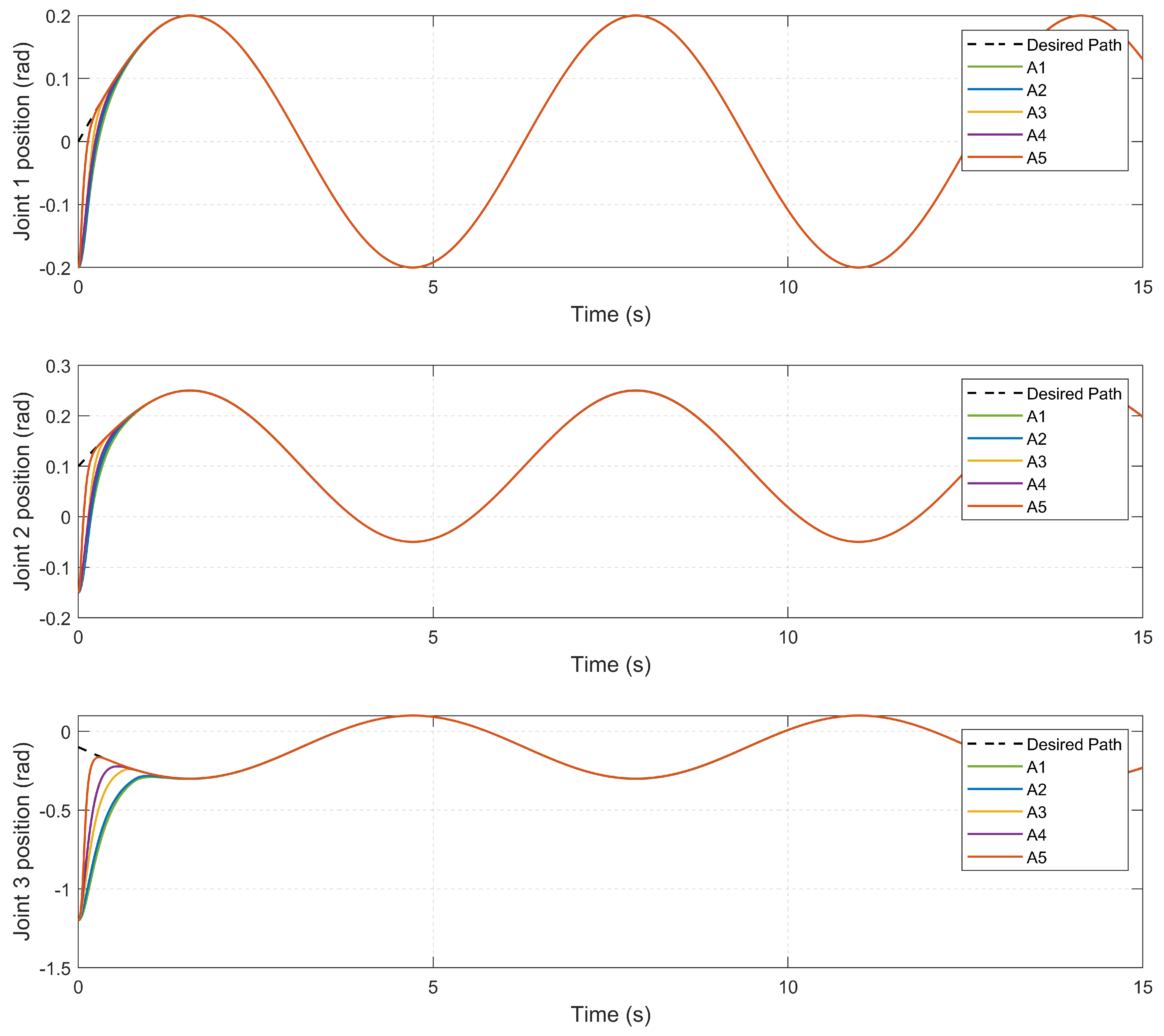
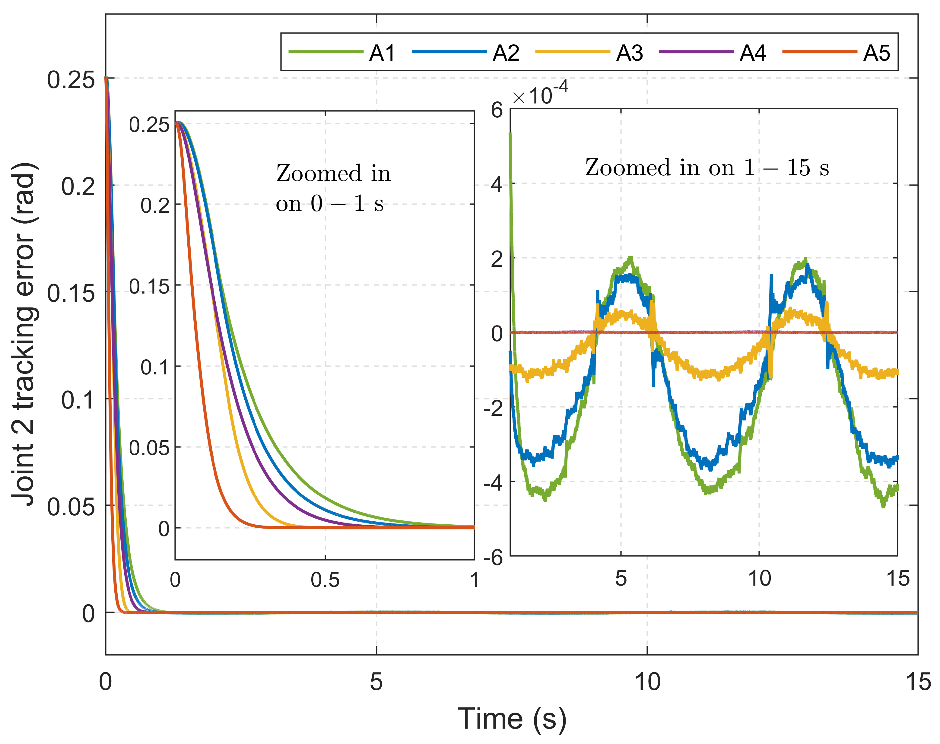
• Case 2: Sinusoidal Trajectory.

  $${\mathit{\eta }}_d\left(t\right)=\left[\begin{array}{c}0.2sin\left(t\right)\\ 0.1+0.15sin\left(t\right)\\ -0.1-0.2sin\left(t\right)\end{array}\right].$$
  To assess robustness against more significant deviations, this scenario uses a larger initial condition $\mathit{\eta }\left(0\right)={[-0.2,-0.15,-1.2]}^T$ (rad), introducing an initial tracking error of approximately $[11.5^{\circ },14.3^{\circ },65.9^{\circ }]$, which is particularly challenging at joint 3. This configuration is intended to rigorously test the controller’s performance under harsh initial conditions.

To quantitatively evaluate tracking performance, two performance indices are employed:

• Root mean square error (RMSE): Used to assess tracking accuracy after the system has converged, specifically in the interval from 1.5 s to 15 s.
• Integral of absolute error (IAE): Used to evaluate the overall accumulated tracking error over time.

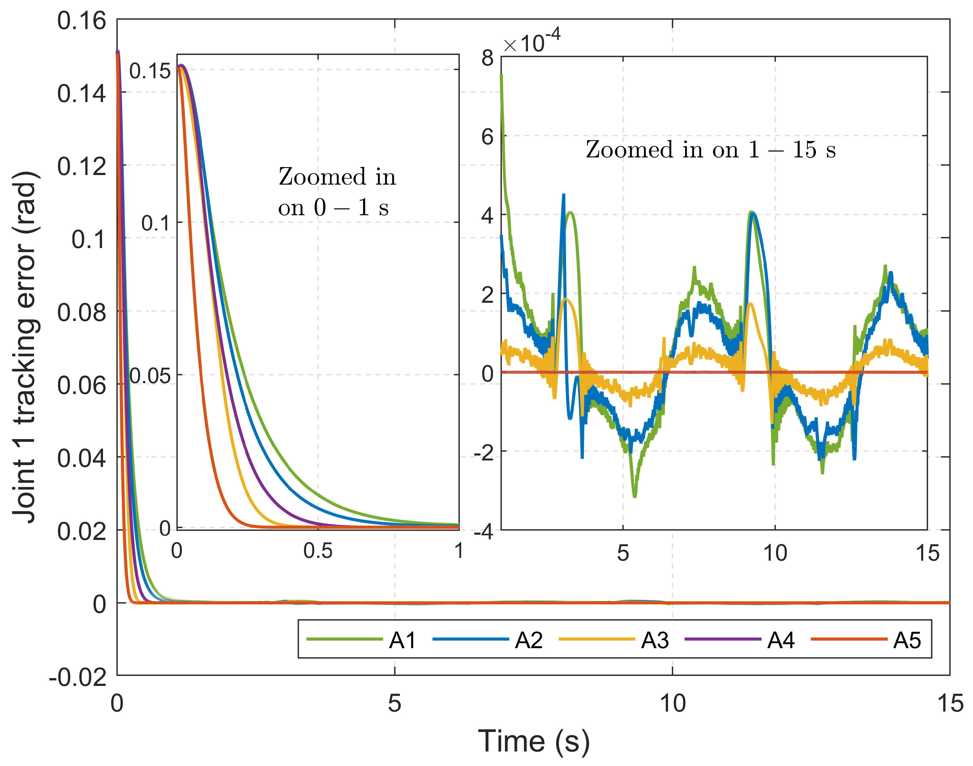
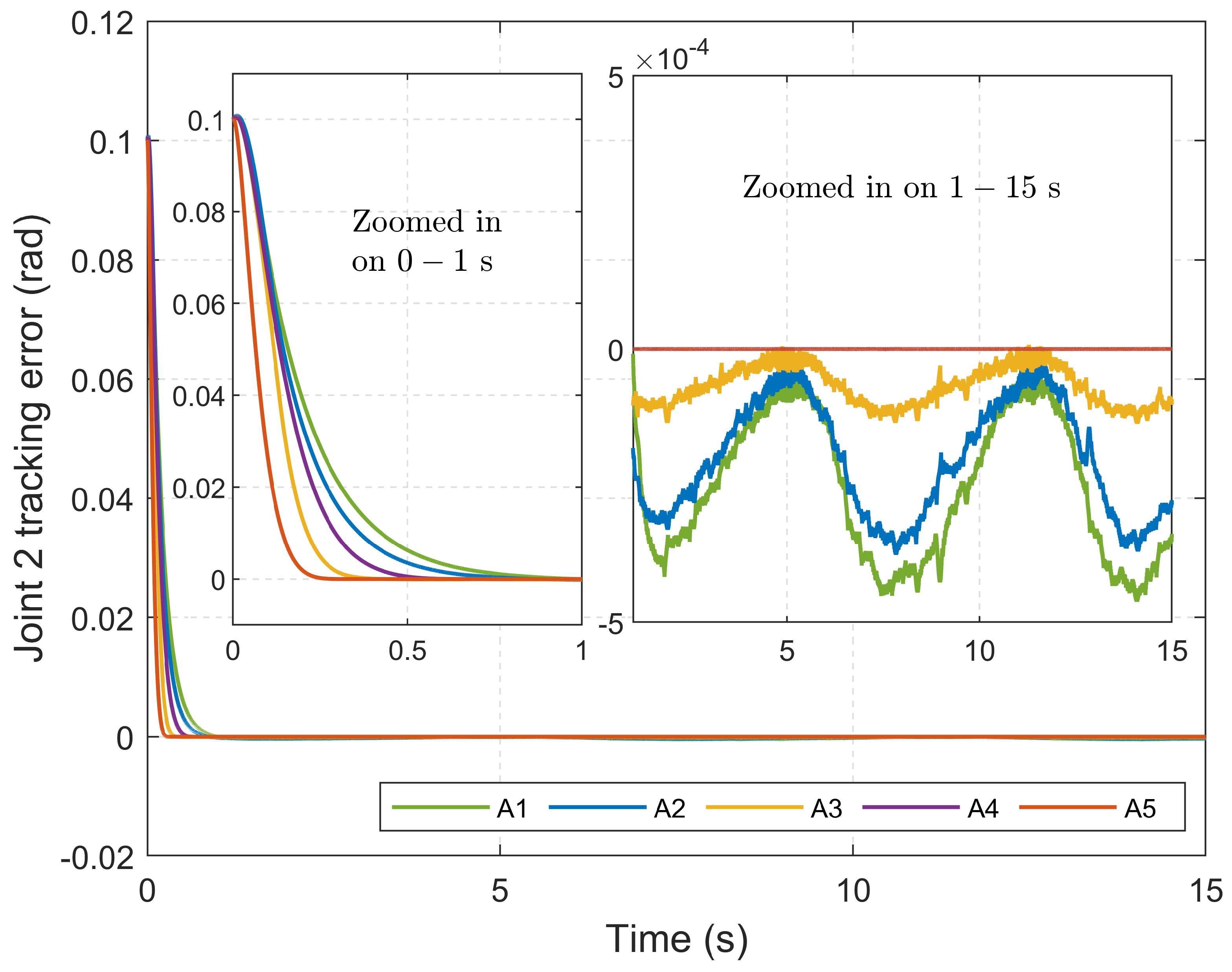
4.4. Tracking Performance: Exponential Reference Trajectory

This subsection presents the simulation results for tracking an exponential reference trajectory under various control strategies. Figure 4, Figure 5, Figure 6, Figure 7, Figure 8 and Figure 9 and

Table 2. RMSE values for different control methods under the exponential reference trajectory.

Method	Joint 1 (rad)	Joint 2 (rad)	Joint 3 (rad)
A1	$1.7798\times {10}^{-4}$	$2.8670\times {10}^{-4}$	$8.5383\times {10}^{-4}$
A2	$1.4341\times {10}^{-4}$	$2.2510\times {10}^{-4}$	$6.9670\times {10}^{-4}$
A3	$5.9288\times {10}^{-5}$	$7.5290\times {10}^{-5}$	$2.2508\times {10}^{-4}$
A4	$1.2065\times {10}^{-7}$	$1.2466\times {10}^{-7}$	$3.3070\times {10}^{-7}$
A5	$3.4777\times {10}^{-8}$	$1.2740\times {10}^{-8}$	$4.7290\times {10}^{-8}$

and

Table 3. IAE values for different control methods under the exponential reference trajectory.

Method	Joint 1 (rad)	Joint 2 (rad)	Joint 3 (rad)
A1	$3.5467\times {10}^{-2}$	$2.4175\times {10}^{-2}$	$3.1753\times {10}^{-2}$
A2	$3.1442\times {10}^{-2}$	$2.1150\times {10}^{-2}$	$2.7591\times {10}^{-2}$
A3	$2.1346\times {10}^{-2}$	$1.3495\times {10}^{-2}$	$1.6126\times {10}^{-2}$
A4	$2.3997\times {10}^{-2}$	$1.5564\times {10}^{-2}$	$1.5612\times {10}^{-2}$
A5	$1.1150\times {10}^{-2}$	$7.4207\times {10}^{-3}$	$7.1914\times {10}^{-3}$

illustrate the performance comparisons in terms of trajectory tracking accuracy, convergence speed, control smoothness, and robustness against disturbances and uncertainties.

Figure 4 shows the tracking trajectories of the manipulator joints under different controllers. All methods successfully track the desired exponential trajectory despite external disturbances, nonlinear friction, and model uncertainties. However, the tracking precision and convergence speed vary significantly among the approaches.

To provide a detailed comparison, the joint tracking errors are shown in Figure 5, Figure 6 and Figure 7. In the initial phase (0–1 s), differences in convergence behavior become apparent. Method A1 exhibits the slowest convergence due to its inherent asymptotic stability characteristic from classical SMC. Method A2 improves on this with finite-time convergence, resulting in faster error reduction.

Methods A3 and A4 achieve even faster convergence due to their fixed-time control frameworks, which guarantee convergence within a fixed time regardless of initial conditions. However, Method A4 shows slightly slower convergence than A3 because it employs a fixed-time observer to estimate and compensate for the combined effects of uncertainties and disturbances, which introduces an additional estimation process. In contrast, the proposed method (Method A5) achieves the fastest convergence. This superior performance is attributed to the combination of a fixed-time control law with the TDE technique, as established in Theorem 1, which provides improved convergence over conventional fixed-time methods with constant parameters.

From the long-term tracking error behavior (1–15 s) depicted in Figure 5, Figure 6 and Figure 7 and summarized in Table 2 and Figure 8a, we observe clear performance distinctions. Method A1 exhibits the largest steady-state tracking errors, with RMSEs of $1.7798\times {10}^{-4}$ rad at joint 1, $2.8670\times {10}^{-4}$ rad at joint 2, and $8.5383\times {10}^{-4}$ rad at joint 3. Method A2 achieves slightly better accuracy, but still with considerable error magnitudes.

Method A3 significantly improves tracking accuracy compared to A2, while Method A4 further reduces the RMSE due to its disturbance estimation mechanism. The best performance is observed with the proposed method, which leverages TDE for dynamic and disturbance compensation. Its RMSE values are notably low: $3.4777\times {10}^{-8}$ rad at joint 1, $1.2740\times {10}^{-8}$ rad at joint 2, and $4.7290\times {10}^{-8}$ rad at joint 3. This demonstrates the method’s outstanding precision and robustness.

To assess cumulative performance over time, the IAE is considered, as shown in Figure 8b and Table 3. Method A1, due to its slow convergence and larger tracking errors, yields the highest IAE values: $3.5467\times {10}^{-2}$ rad (joint 1), $2.4175\times {10}^{-2}$ rad (joint 2), and $3.1753\times {10}^{-2}$ rad (joint 3). Method A2 slightly improves upon this, but still shows moderate error accumulation.

Method A3 achieves lower IAE values: $2.1346\times {10}^{-2}$, $1.3495\times {10}^{-2}$, and $1.6126\times {10}^{-2}$ rad at joints 1 to 3, respectively. Interestingly, although Method A4 offers better tracking accuracy than A3, its IAE values at joints 1 and 2 are slightly higher due to slower initial convergence. Nonetheless, Method A4 maintains strong performance overall.

The proposed method achieves the lowest IAE values across all joints: $1.1150\times {10}^{-2}$ rad at joint 1, $7.4207\times {10}^{-3}$ rad at joint 2, and $7.1914\times {10}^{-3}$ rad at joint 3. This highlights its capacity to effectively minimize both transient and steady-state errors.

Finally, Figure 9 illustrates the control torque signals generated by each method. Methods A1, A2, and A3 exhibit noticeable chattering due to high sliding gains, which are typically set conservatively above the worst-case uncertainty bounds. Such high-frequency switching leads to mechanical wear, system vibrations, and increased energy consumption, which are undesirable for practical applications.

In contrast, Methods A4 and the proposed Method A5 demonstrate significantly smoother control signals. Method A4 achieves this by using low sliding gains to correct only the observer’s estimation error. Similarly, the proposed method uses a small gain to compensate for the residual estimation error of the TDE. This smooth control behavior is crucial for improving energy efficiency and prolonging the lifespan of mechanical and electrical components.

4.5. Tracking Performance: Sinusoidal Reference Trajectory

The simulation results for the sinusoidal desired trajectory are presented in Figure 10, Figure 11, Figure 12, Figure 13, Figure 14 and Figure 15 and

Table 4. RMSE values for different control methods under the sinusoidal reference trajectory.

Method	Joint 1 (rad)	Joint 2 (rad)	Joint 3 (rad)
A1	$1.3462\times {10}^{-4}$	$2.7941\times {10}^{-4}$	$8.5973\times {10}^{-4}$
A2	$1.0412\times {10}^{-4}$	$2.2634\times {10}^{-4}$	$6.8676\times {10}^{-4}$
A3	$3.7197\times {10}^{-5}$	$7.4778\times {10}^{-5}$	$2.2104\times {10}^{-4}$
A4	$1.0813\times {10}^{-7}$	$4.3409\times {10}^{-7}$	$7.8118\times {10}^{-7}$
A5	$6.4364\times {10}^{-8}$	$7.1679\times {10}^{-8}$	$6.0078\times {10}^{-8}$

and

Table 5. IAE values for different control methods under the sinusoidal reference trajectory.

Method	Joint 1 (rad)	Joint 2 (rad)	Joint 3 (rad)
A1	$4.8594\times {10}^{-2}$	$6.0910\times {10}^{-2}$	$4.0874\times {10}^{-1}$
A2	$4.2631\times {10}^{-2}$	$5.4865\times {10}^{-2}$	$3.7890\times {10}^{-1}$
A3	$2.9857\times {10}^{-2}$	$3.7754\times {10}^{-2}$	$2.5806\times {10}^{-1}$
A4	$3.4774\times {10}^{-2}$	$4.3124\times {10}^{-2}$	$1.9613\times {10}^{-1}$
A5	$1.5562\times {10}^{-2}$	$1.9558\times {10}^{-2}$	$1.0985\times {10}^{-1}$

. This scenario is intentionally designed with large initial tracking errors, particularly at joint 3, to rigorously test the controllers’ robustness under challenging operating conditions. These results further validate the effectiveness of the proposed control method in the presence of disturbances and model uncertainties.

Figure 10 illustrates the joint trajectory tracking performance of all control strategies. It can be observed that all methods enable the system to follow the desired sinusoidal trajectory despite the existence of external disturbances and uncertainties. However, the response characteristics differ significantly among methods.

To examine the tracking behavior in more detail, Figure 11, Figure 12 and Figure 13 show the joint tracking errors over time. From the enlarged plots in the initial interval (0–1 s) and the RMSE values reported in Figure 14a and Table 4, a consistent performance trend is observed, mirroring the pattern from the exponential trajectory case.

Method A1 exhibits the slowest convergence due to its asymptotic stability nature. Method A2 achieves improved transient response via finite-time convergence. Methods A3 and A4 further enhance the convergence rate, benefiting from fixed-time convergence properties. Although both methods target fixed-time stability, A4 utilizes a fixed-time disturbance observer to estimate and cancel out uncertainties, which slightly delays its response compared to A3 in scenarios with small to moderate initial errors.

However, a notable observation emerges under large initial error conditions. As shown in Figure 13, Method A4 achieves faster convergence than Method A3 at joint 3, where the initial deviation is particularly high. This highlights the strength of Method A4 in situations far from equilibrium. One key reason for this behavior is that A4’s disturbance observer provides more accurate compensation for the nonlinear terms and external perturbations, which become more pronounced when the system starts far from the desired trajectory. In contrast, Method A3, which lacks an active disturbance estimation mechanism, becomes more sensitive to high initial mismatches, leading to slower recovery in such cases.

The proposed method achieves the fastest convergence among all approaches, attributed to its use of a model-free TDE technique and a robust fixed-time control structure based on Theorem 1.

Regarding tracking accuracy, a similar pattern is observed. Method A1 has the highest steady-state error, indicating the lowest tracking precision. Method A2 offers slightly better accuracy than A1. Method A3 significantly improves the tracking precision, while Method A4 further enhances accuracy due to effective disturbance compensation using the observer. The proposed method consistently delivers the best tracking accuracy across all joints. This improvement is attributed to the combination of the TDE-based estimation of dynamics and disturbances and the robust fixed-time convergence mechanism, which together ensure minimal tracking errors under varying conditions.

The IAE values in Figure 14b and Table 5 further confirm this trend. Method A1 exhibits the highest accumulated error, followed by A2 and A3. While Method A4 generally performs better than A3 in terms of steady-state accuracy, its slightly delayed convergence at joints 1 and 2 results in higher IAE values at those joints. Nevertheless, Method A4 shows superior IAE performance at Joint 3, where the initial error is largest, owing to its faster recovery in that case. Overall, the proposed method achieves the lowest IAE across all joints, combining fast convergence with minimal steady-state error.

Figure 15 presents the control torque signals generated by each method. As seen in the figure, Methods A1, A2, and A3 generate control inputs with noticeable chattering effects. These high-frequency oscillations result from the use of large sliding gains, typically set conservatively above the upper bounds of uncertainties to ensure robustness. However, such signals can cause mechanical wear, induce vibrations, and increase energy consumption. In contrast, Method A4 and the proposed method (A5) produce significantly smoother control signals. This extends the lifetime of actuators and reduces undesired system vibrations.

In summary, the simulation results reaffirm the superior performance of the proposed control method. It not only achieves the fastest convergence and the highest tracking accuracy but also generates smooth control signals, making it highly effective for practical applications in robotic systems. The consistent outperformance across both the exponential and sinusoidal reference trajectory scenarios strongly supports the robustness and reliability of the proposed strategy. Furthermore, by employing a model-free control framework, the proposed method eliminates the need for precise knowledge of the system dynamics, significantly enhancing its adaptability and ease of implementation in real-world scenarios with uncertain or varying system parameters.

5. Conclusions

This paper presented a novel MF-NFxTSMC algorithm for trajectory tracking in robotic arm systems. By employing TDE to estimate system dynamics and external disturbances in real-time, the proposed approach eliminates the need for accurate mathematical models. The introduced SF-FxTSS incorporates a dynamic proportional term and an adaptive exponent, ensuring robust fixed-time convergence independent of initial conditions. Additionally, a smooth FxTRL was designed to suppress chattering while preserving strong convergence guarantees. The fixed-time stability of the closed-loop system was rigorously verified through Lyapunov-based analysis. Numerical simulations conducted on the SAMSUNG FARA AT2 robotic platform demonstrated the proposed controller’s superiority over conventional SMC, finite-time SMC, approximate fixed-time SMC, and global fixed-time NTSMC, in terms of tracking accuracy, convergence speed, and smoothness of control.

Despite these promising results, several limitations remain. The proposed method has so far been validated only through simulations, without experimental testing on physical robotic hardware. Although the TDE mechanism enhances robustness, its estimation accuracy may degrade under high levels of sensor noise. Moreover, the current approach requires manual parameter tuning, which may hinder scalability to more complex systems. Future research will focus on addressing these limitations by conducting experimental validation under real-world constraints, such as actuator saturation, sensor noise, and unmodeled dynamics. Enhancing the noise robustness of the TDE structure and incorporating learning- or optimization-based techniques for automatic parameter tuning are also key directions. In addition, integrating the proposed framework with advanced perception systems and reinforcement learning strategies will be investigated to enable autonomous and adaptive manipulation in unstructured environments.

References

1. Jin, M.; Kang, S.H.; Chang, P.H.; Lee, J. Robust control of robot manipulators using inclusive and enhanced time delay control. IEEE/ASME Trans. Mechatron. 2017, 22, 2141–2152. [Google Scholar] [CrossRef]
2. Kali, Y.; Saad, M.; Boland, J.F.; Fortin, J.; Girardeau, V. Walking task space control using time delay estimation based sliding mode of position controlled nao biped robot. Int. J. Dyn. Control 2021, 9, 679–688. [Google Scholar] [CrossRef]
3. Lee, J.E.; Kim, B.W. Research on Direct Yaw Moment Control Based on Neural Sliding Mode Control for Four-Wheel Actuated Electric Vehicles. In Proceedings of the 2023 IEEE 6th International Conference on Knowledge Innovation and Invention (ICKII), Sapporo, Japan, 11–13 August 2023; pp. 736–740. [Google Scholar]
4. Kali, Y.; Saad, M.; Benjelloun, K.; Benbrahim, M. Sliding mode with time delay control for robot manipulators. In Applications of Sliding Mode Control; Springer: Berlin/Heidelberg, Germany, 2017; pp. 135–156. [Google Scholar]
5. Taheri, E.; Ferdowsi, M.H.; Danesh, M. Design boundary layer thickness and switching gain in SMC algorithm for AUV motion control. Robotica 2019, 37, 1785–1803. [Google Scholar] [CrossRef]
6. Fateh, A.; Momeni, H. Time delay control of a robotic manipulator using an enhanced adaptive sliding mode control switching gain. Int. J. Dyn. Control 2025, 13, 91. [Google Scholar] [CrossRef]
7. Truong, T.N.; Vo, A.T.; Kang, H.J. A Novel Time Delay Nonsingular Fast Terminal Sliding Mode Control for Robot Manipulators with Input Saturation. Mathematics 2024, 13, 119. [Google Scholar] [CrossRef]
8. Song, T.; Fang, L.; Wang, H. Model-free finite-time terminal sliding mode control with a novel adaptive sliding mode observer of uncertain robot systems. Asian J. Control 2022, 24, 1437–1451. [Google Scholar] [CrossRef]
9. Ahmed, S.; Wang, H.; Tian, Y. Adaptive high-order terminal sliding mode control based on time delay estimation for the robotic manipulators with backlash hysteresis. IEEE Trans. Syst. Man, Cybern. Syst. 2019, 51, 1128–1137. [Google Scholar] [CrossRef]
10. Brahmi, B.; Driscoll, M.; Laraki, M.H.; Brahmi, A. Adaptive high-order sliding mode control based on quasi-time delay estimation for uncertain robot manipulator. Control Theory Technol. 2020, 18, 279–292. [Google Scholar] [CrossRef]
11. Boudjedir, C.E.; Bouri, M.; Boukhetala, D. An enhanced adaptive time delay control-based integral sliding mode for trajectory tracking of robot manipulators. IEEE Trans. Control Syst. Technol. 2022, 31, 1042–1050. [Google Scholar] [CrossRef]
12. Park, J.; Kwon, W.; Park, P. An improved adaptive sliding mode control based on time-delay control for robot manipulators. IEEE Trans. Ind. Electron. 2022, 70, 10363–10373. [Google Scholar] [CrossRef]
13. Meng, D.; Xu, H.; Xu, H.; Sun, H.; Liang, B. Trajectory tracking control for a cable-driven space manipulator using time-delay estimation and nonsingular terminal sliding mode. Control Eng. Pract. 2023, 139, 105649. [Google Scholar] [CrossRef]
14. Truong, T.N.; Vo, A.T.; Kang, H.J. Real-time implementation of the prescribed performance tracking control for magnetic levitation systems. Sensors 2022, 22, 9132. [Google Scholar] [CrossRef]
15. Yu, X.; Feng, Y.; Man, Z. Terminal sliding mode control–an overview. IEEE Open J. Ind. Electron. Soc. 2020, 2, 36–52. [Google Scholar] [CrossRef]
16. Sun, C.; Huang, Z.; Wu, H. Adaptive super-twisting global nonsingular terminal sliding mode control for robotic manipulators. Nonlinear Dyn. 2024, 112, 5379–5389. [Google Scholar] [CrossRef]
17. Hu, S.; Wan, Y.; Liang, X. Adaptive nonsingular fast terminal sliding mode trajectory tracking control for robotic manipulators with model feedforward compensation. Nonlinear Dyn. 2025, 113, 16893–16911. [Google Scholar] [CrossRef]
18. Lee, J.E.; Kim, B.W. A Novel Adaptive Non-Singular Fast Terminal Sliding Mode Control for Direct Yaw Moment Control in 4WID Electric Vehicles. Sensors 2025, 25, 941. [Google Scholar] [CrossRef]
19. Vo, A.T.; Truong, T.N.; Kang, H.J.; Le, T.D. A fixed-time sliding mode control for uncertain magnetic levitation systems with prescribed performance and anti-saturation input. Eng. Appl. Artif. Intell. 2024, 133, 108373. [Google Scholar] [CrossRef]
20. Lee, J.E.; Kim, B.W. Improving Direct Yaw-Moment Control via Neural-Network-Based Non-Singular Fast Terminal Sliding Mode Control for Electric Vehicles. Sensors 2024, 24, 4079. [Google Scholar] [CrossRef]
21. Lee, J.E.; Kim, B.W. A DYC system for 4WID Electric Vehicles via Fuzzy-Nonsingular Fast Terminal Sliding Mode Control. In Proceedings of the 2025 IEEE International Conference on Mechatronics (ICM), Wollongong, Australia, 28 February–2 March 2025; pp. 1–6. [Google Scholar]
22. Zhang, Y.; Yang, X.; Wei, P.; Liu, P.X. Fractional-order adaptive non-singular fast terminal sliding mode control with time delay estimation for robotic manipulators. IET Control Theory Appl. 2020, 14, 2556–2565. [Google Scholar] [CrossRef]
23. Labbadi, M.; Muñoz-Vázquez, A.; Djemai, M.; Boukal, Y.; Zerrougui, M.; Cherkaoui, M. Fractional-order nonsingular terminal sliding mode controller for a quadrotor with disturbances. Appl. Math. Model. 2022, 111, 753–776. [Google Scholar] [CrossRef]
24. Liu, Y.; Li, H.; Lu, R.; Zuo, Z.; Li, X. An overview of finite/fixed-time control and its application in engineering systems. IEEE/CAA J. Autom. Sin. 2022, 9, 2106–2120. [Google Scholar] [CrossRef]
25. Sai, H.; Xu, Z.; He, S.; Zhang, E.; Zhu, L. Adaptive nonsingular fixed-time sliding mode control for uncertain robotic manipulators under actuator saturation. ISA Trans. 2022, 123, 46–60. [Google Scholar] [CrossRef]
26. Zhang, D.; Hu, J.; Cheng, J.; Wu, Z.G.; Yan, H. A novel disturbance observer based fixed-time sliding mode control for robotic manipulators with global fast convergence. IEEE/CAA J. Autom. Sin. 2024, 11, 661–672. [Google Scholar] [CrossRef]
27. Khodaverdian, M.; Hajshirmohamadi, S.; Hakobyan, A.; Ijaz, S. Predictor-based constrained fixed-time sliding mode control of multi-UAV formation flight. Aerosp. Sci. Technol. 2024, 148, 109113. [Google Scholar] [CrossRef]
28. Xu, R.; Tian, D.; Wang, Z. Adaptive disturbance observer-based local fixed-time sliding mode control with an improved approach law for motion tracking of piezo-driven microscanning system. IEEE Trans. Ind. Electron. 2024, 71, 12824–12834. [Google Scholar] [CrossRef]
29. Anjum, Z.; Zhou, H.; Ahmed, S.; Guo, Y. Fixed time sliding mode control for disturbed robotic manipulator. J. Vib. Control 2024, 30, 1580–1593. [Google Scholar] [CrossRef]
30. Truong, T.N.; Vo, A.T.; Kang, H.J. Neural network-based sliding mode controllers applied to robot manipulators: A review. Neurocomputing 2023, 562, 126896. [Google Scholar] [CrossRef]
31. Levant, A. Chattering analysis. IEEE Trans. Autom. Control 2010, 55, 1380–1389. [Google Scholar] [CrossRef]
32. Zuo, Z. Non-singular fixed-time terminal sliding mode control of non-linear systems. IET Control Theory Appl. 2015, 9, 545–552. [Google Scholar] [CrossRef]
33. Gao, Z.; Zhang, Y.; Guo, G. Fixed-Time Prescribed Performance Adaptive Fixed-Time Sliding Mode Control for Vehicular Platoons with Actuator Saturation. IEEE Trans. Intell. Transp. Syst. 2022, 23, 24176–24189. [Google Scholar] [CrossRef]
34. Su, Y.; Zheng, C.; Mercorelli, P. Robust approximate fixed-time tracking control for uncertain robot manipulators. Mech. Syst. Signal Process. 2020, 135, 106379. [Google Scholar] [CrossRef]
35. Yu, L.; He, G.; Wang, X.; Shen, L. A novel fixed-time sliding mode control of quadrotor with experiments and comparisons. IEEE Control Syst. Lett. 2021, 6, 770–775. [Google Scholar] [CrossRef]
36. Li, H.; Cai, Y. Fixed-time non-singular terminal sliding mode control with globally fast convergence. IET Control Theory Appl. 2022, 16, 1227–1241. [Google Scholar] [CrossRef]
37. Lee, J.; Chang, P.H.; Jin, M. Adaptive integral sliding mode control with time-delay estimation for robot manipulators. IEEE Trans. Ind. Electron. 2017, 64, 6796–6804. [Google Scholar] [CrossRef]
38. Truong, T.N.; Vo, A.T.; Kang, H.J. A model-free terminal sliding mode control for robots: Achieving fixed-time prescribed performance and convergence. ISA Trans. 2024, 144, 330–341. [Google Scholar] [CrossRef]
39. Sun, G.; Zeng, Q. A Finite-Time Sliding Mode Control Approach for Constrained Euler–Lagrange System. Mathematics 2023, 11, 2788. [Google Scholar] [CrossRef]
Figure 1. Convergence behavior under different initial conditions of fixed-time systems and their convergence times.
Mathematics 13 01579 g001
Figure 2. Proposed control system.
Mathematics 13 01579 g002
Figure 3. Three-dimensional SolidWorks model of the Samsung FARA AT2 robotic arm.
Mathematics 13 01579 g003
Figure 4. Comparative trajectory tracking performance of all methods for exponential reference trajectory at joints.
Mathematics 13 01579 g004
Figure 5. Comparative tracking errors for all methods at Joint 1 under the exponential reference trajectory.
Mathematics 13 01579 g005
Figure 6. Comparative tracking errors for all methods at Joint 2 under the exponential reference trajectory.
Mathematics 13 01579 g006
Figure 7. Comparative tracking errors for all methods at Joint 3 under the exponential reference trajectory.
Mathematics 13 01579 g007
Figure 8. Comparison of RSME and IAE for different controllers under the exponential reference trajectory.
Mathematics 13 01579 g008
Figure 9. Control inputs at joints for all methods under the exponential reference trajectory.
Mathematics 13 01579 g009
Figure 10. Comparative trajectory tracking performance of all methods for sinusoidal reference trajectory at joints.
Mathematics 13 01579 g010
Figure 11. Comparative tracking errors for all methods at Joint 1 under the sinusoidal reference trajectory.
Mathematics 13 01579 g011
Figure 12. Comparative tracking errors for all methods at Joint 2 under the sinusoidal reference trajectory.
Mathematics 13 01579 g012
Figure 13. Comparative tracking errors for all methods at Joint 3 under the sinusoidal reference trajectory.
Mathematics 13 01579 g013
Figure 14. Comparison of RSME and IAE for different controllers under the sinusoidal reference trajectory.
Mathematics 13 01579 g014
Figure 15. Control inputs at joints for all methods under the sinusoidal reference trajectory.
Mathematics 13 01579 g015