
A Pretrained Spatio-Temporal Hypergraph Transformer for Multi-Stock Trend Forecasting


Abstract
1. Introduction
- Traditional methods rely on simple correlations between stock pairs, without considering the complex high-order relationships among multiple stocks. This leads to an inability to capture the complex dynamic relationships in the stock market and results in inefficient utilization of available data.
- Newly listed stocks usually lack historical data, which poses a cold-start problem for traditional models that heavily rely on historical sequence modeling. Pretraining methods, while promising in other fields, face challenges in stock prediction due to the heterogeneous behavior of different stocks. This highlights the need for more adaptive pretraining frameworks tailored to financial data.
- We propose a spatio-temporal hypergraph transformer for stock trend prediction. The network considers the temporal correlation of each stock through a temporal encoder, and the spatial correlation between stocks through a hybrid attention hypergraph module, which consists of self-attention and cross-attention mechanisms. The self-attention dynamically generates hyperedges, while the cross-attention performs convolution operations on the hypergraph associations to model complex and high-order stock relationships.
- We design an efficient pretraining and fine-tuning framework, employing a pretraining task that reconstructs masked time series to enhance the model’s generalization ability and reduce its dependency on historical data, thereby making it applicable to newly listed stocks with limited available samples.
- Experiments on the CSI300 and NASDAQ100 datasets demonstrated the effectiveness of STHformer, with superior predictive performance and long-term profitability compared to several state-of-the-art solutions.
2. Related Work
2.1. Spatial-Temporal Models
2.2. Self-Supervised Pretraining in Time Series Modeling
2.3. Stock Price Forecasting
3. Preliminary
Problem Formulation
- Stock Trend Forecasting: Assuming that there are N stocks in the stock market, a set of historical sequence data at day t is represented by , where T is the length of the sequence, and F is the dimension of the original feature, such as open, high, low, close and volume. Each stock i has historical sequence data at day t. If the closing price of stock is higher than the opening price of , the stock is labeled with “up” (), otherwise it is labeled with “down” (), where h is a specified horizon ahead of the current timestamp. The objective of stock trend forecasting is to establish a mapping relationship, which is defined as follows:where is the input stock sequence data and , is the predicted trend for all stocks at day t+h.
- Hypergraph: A hypergraph is constructed to model the interdependence among stocks, where the hyperedges encode higher-order relationships between them. The collection of vertices is denoted by V, while the set of hyperedges is represented by E. Each hyperedge is associated with a positive weight w, and these weights are collectively organized in a diagonal matrix .
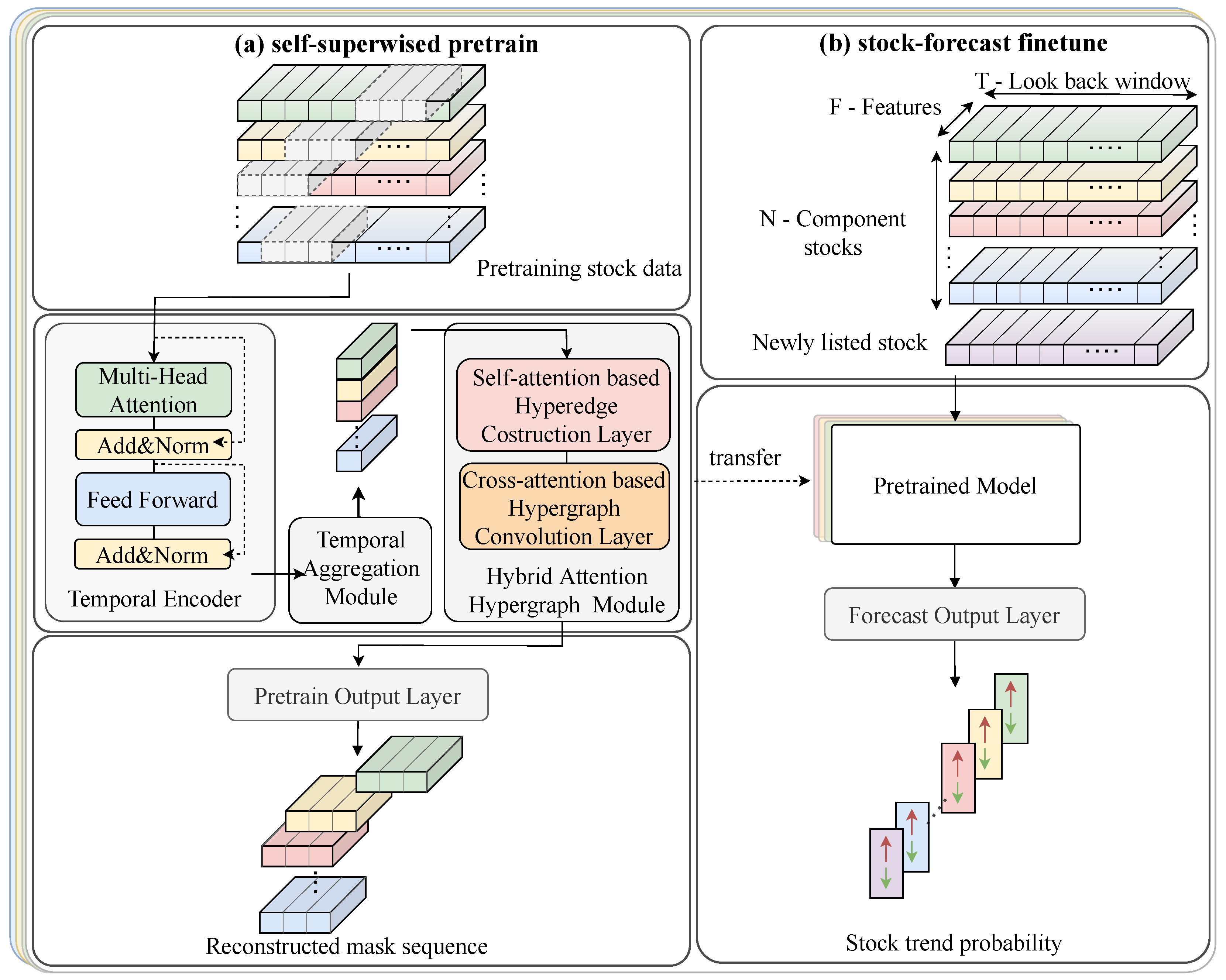
4. Model
- Temporal Encoder: This module employs a Transformer encoder to extract the temporal correlations in each stock’s daily data.
- Temporal Aggregation Module: This module integrates information across various time points to produce a localized embedding. This embedding captures all significant signals along the temporal axis, while maintaining the intricate local details of the stock’s behavior over time
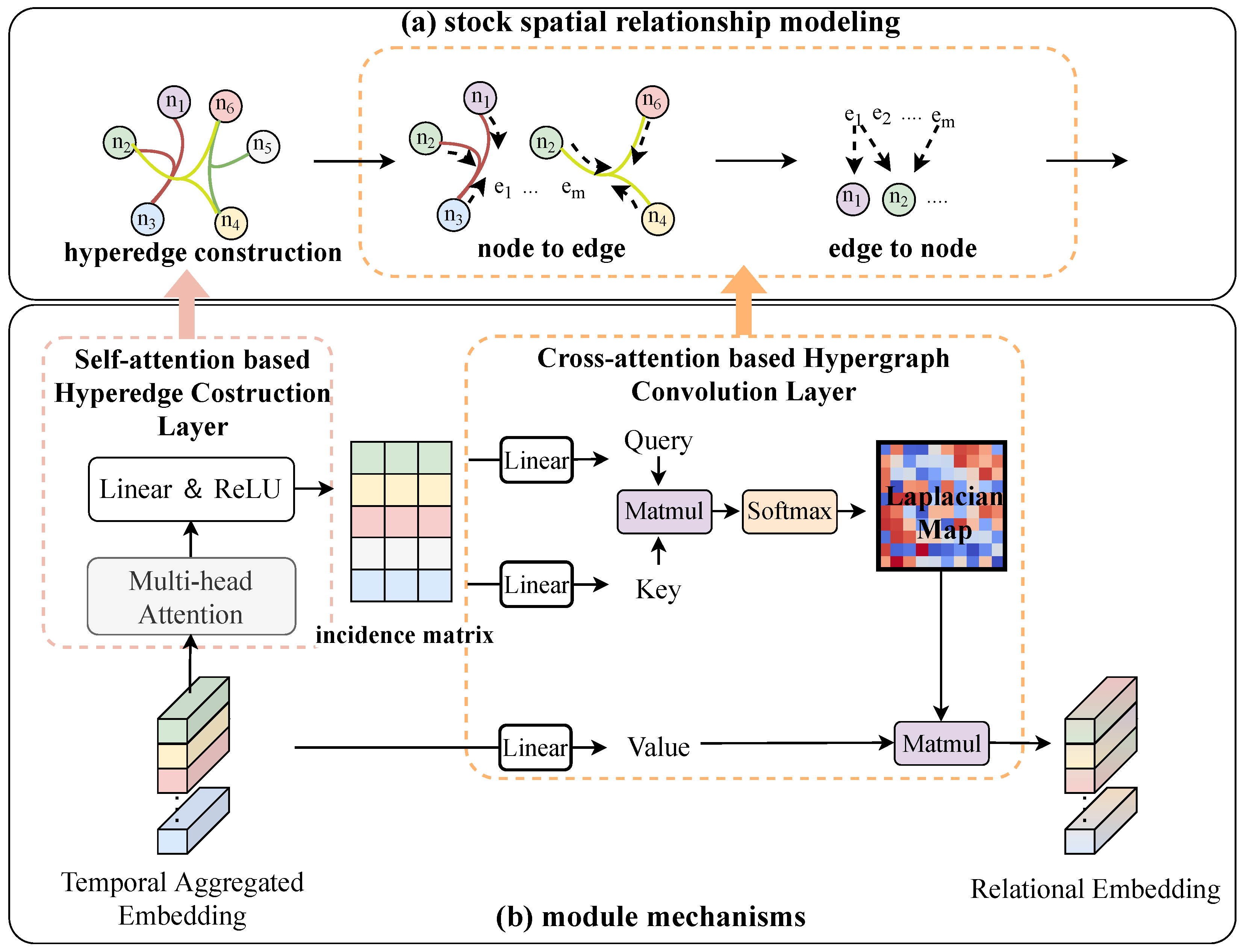
- Hybrid Attention Hypergraph Module: This module is designed to explore the spatial relationships between stocks. It comprises two attention layers: the self-attention-based hyperedge construction layer dynamically generates hyperedges, while the cross-attention-based hypergraph convolution layer performs hypergraph convolution on stock nodes based on the generated hyperedge matrix.
- Self-Supervised Pretraining Scheme: This strategy involves reconstructing the original time series from the masked time series, with the objective of learning the valuable low-level information from data in an unsupervised manner.
4.1. Temporal Encoder
4.2. Temporal Aggregation Module
4.3. Hybrid Attention Hypergraph Module
4.3.1. Self-Attention-Based Hyperedge Construction Layer
4.3.2. Cross-Attention-Based Hypergraph Convolution Layer
4.4. Self-Supervised Pretraining Scheme
| Algorithm 1 The pretraining algorithm of STHformer |
|
4.5. Fine-Tuning Scheme Tailored for Stock Price Classification
| Algorithm 2 The fine-tuning algorithm of STHformer |
|
5. Experiments and Analysis
5.1. Experimental Settings
5.1.1. Dataset
5.1.2. Evaluation Metrics
- Accuracy:where TP stands for true positive, TN for true negative, FP for false positive, and FN for false negative.
- Recall:
- F1-score:
- AR: The annualized return measures the geometric mean growth rate of an investment portfolio over a one-year period, reflecting its compounded profitability. In our experiment, we computed AR based on 252 trading days per year.where N denotes the total number of trading days in the evaluation period, and is the daily return on day n.
- SR: Sharpe ratio quantifies a portfolio’s risk-adjusted performance by comparing its excess return to its return volatility. Mathematically, it is defined aswhere is the sequence of portfolio returns. To ensure comparability across time horizons, we annualized the ratio as follows:
- MDD: Maximum drawdown measures the short-term loss in cumulative portfolio value.where and represent the cumulative return at moment i and moment j, respectively.
5.1.3. Compared Methods
- Transformer [8]: Transformer uses a self-attention mechanism along the time axis to present global information in the input data.
- GATs [6]: A graph-based baseline, which utilizes graph attention networks to model the relationships between different stocks.
- PatchTST [27]: A Transformer-based model which utilizes channel independence to handle multivariate time series and employs patch technology to extract local semantic information from the time series.
- StockMixer [38]: A MLP-based model, which consists of indicator mixing, time mixing, and stock mixing to capture the complex correlations in stock data.
- DTSMLA [23]: A multi-level attention prediction model, which considers the influence of the market on stock through a gating mechanism and uses a multi-task process to predict price changes.
- MASTER [33]: A Transformer-based model, which introduces a gating mechanism to integrate market information and mines the cross-time stock correlation with learning-based methods.
5.1.4. Backtesting Settings
- Cost: A trading cost distribution of 0.1% was applied to CSI300 and NASDAQ100.
- Trading Period: The backtesting period spanned from 1 April 2020 to 1 May 2024.
- Select Stocks: The strategy selected the top 10% stocks with the highest predicted probability of price appreciation for trading day t.
- Initial Funding and Position Distribution: We assumed an initial capital of 10 million units of the local currency. Portfolio weights were allocated equally among all selected stocks, maintaining uniform position sizing.
- Trading Strategy: The strategy established equal-weighted long positions in all selected stocks at the closing price of day t, maintaining these positions for a fixed 15-trading-day horizon before liquidating at the closing price on day . In the next trading period, the strategy was repeated. It is noteworthy that, due to the recent overall bear market of the CSI300 Index, we introduced a stop-loss mechanism in our trading. This mechanism terminated the current buy–sell transaction when the maximum drawdown within the period exceeded the threshold , which was set to 0.1 in our experiment.
5.2. Hyperparameter Settings
- Transformer [8]: We tuned the number of hidden layers within {32, 64, 128} for encoding layers and tested the number of parallel attention heads within {2, 4, 8}.
- GATS [6]: We tuned the number of hidden units within {32, 64, 128} and the number of layers within {1, 2, 3}, respectively.
- PatchTST [27]: We followed the original settings in the works, tuning the numbers of hidden layer width within {32, 64, 128} and tuning the patch length within {5, 10, 15}, respectively.
- StockMixer [38]: We followed the original settings in the works, tuning the number of market dimensions within {10, 20, 30} and tuning the multi-scale factor within {1, 2, 3, 4}, respectively.
- DTSMLA [23]: We followed the original settings in the work and tuned the number of attention heads within {2, 4, 8}.
- MASTER [33]: We maintained the original architecture of the model, tuning the number of attention heads in the intra-stock layer within {2, 4, 8} and tuning the number of attention heads in the inter-stock layer within {2, 4, 8}, respectively.
5.3. Performance Comparison
5.3.1. Predictive Performance
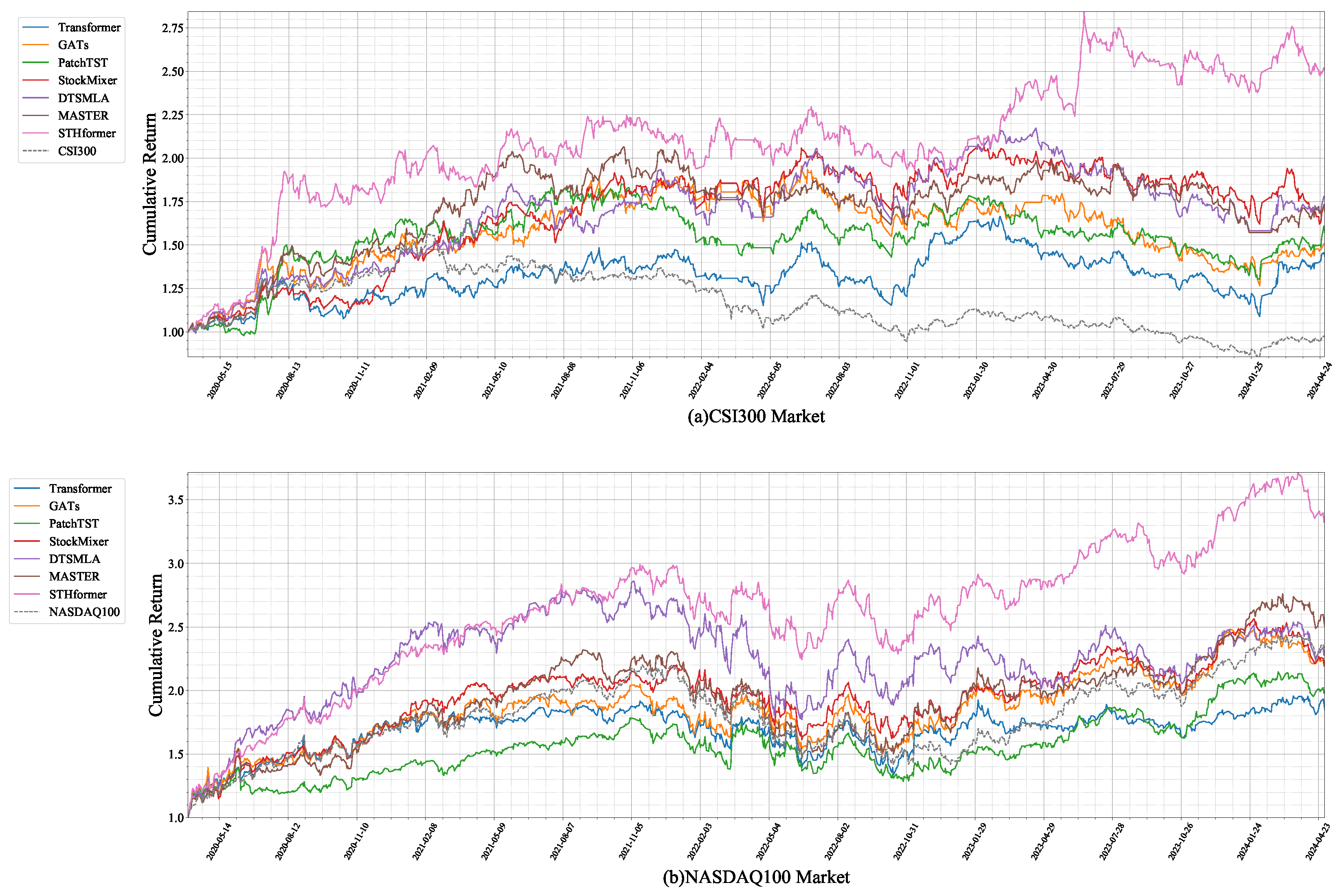
5.3.2. Backtesting Performance
5.4. Model Stability Performance
5.5. Ablation Study
- STHformer w/o HA & Pre: The hybrid attention module and pretraining process in STHformer was removed and all other components were retained.
- STHformer w/o HA: The hybrid attention module in STHformer was removed and all other components were retained.
- STHformer w/o Pre: The pretraining process in STHformer was removed and all other components were retained.
5.5.1. Effectiveness of Hybrid Attention Module
5.5.2. Effectiveness of Pretraining Strategy
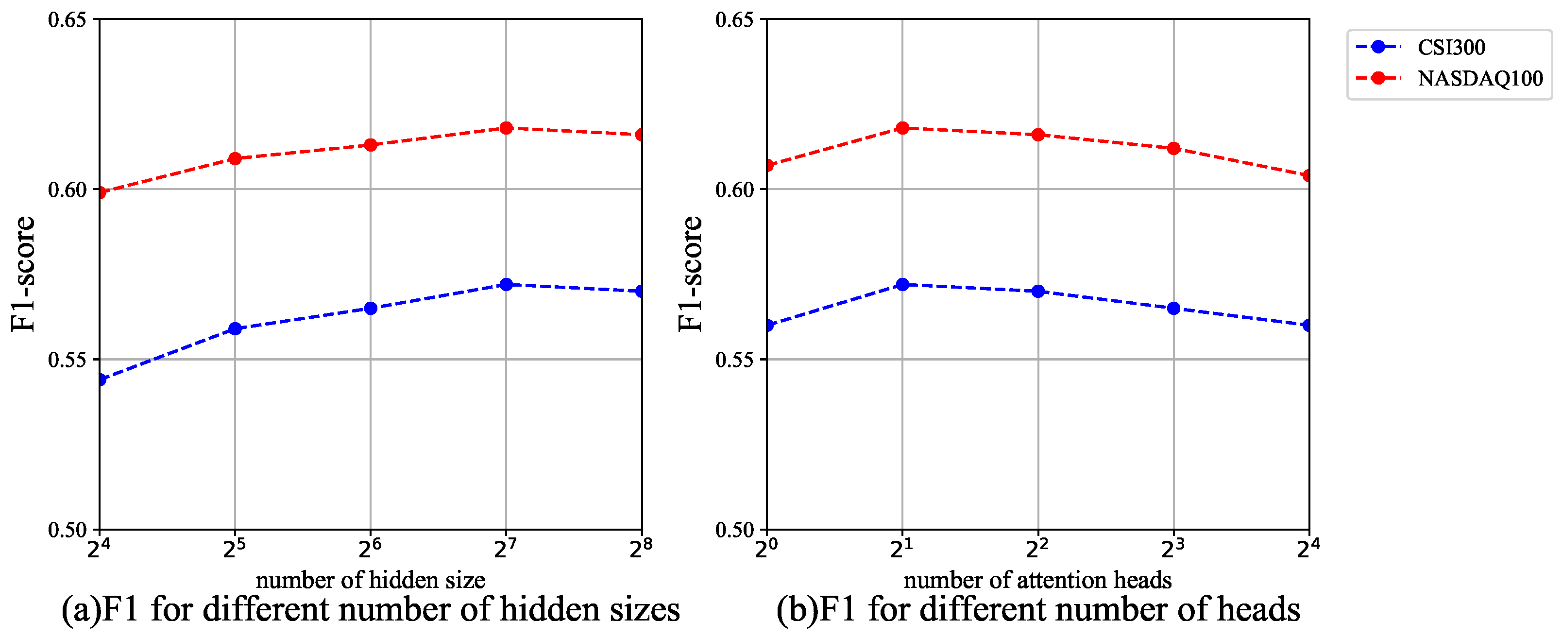
5.6. Parameter Analysis
- Number of hidden sizes: Figure 5a shows the comparison of F1 scores for the STHformer model with different hidden layer sizes. The experimental results indicate that the model achieved the best predictive performance when the hidden layer size was set to . It is worth noting that as the hidden layer size was increased further, the predictive performance of STHformer tended to stabilize. Based on this analysis, this chapter adopted as the optimal hidden layer configuration for the model.
- Number of heads: Figure 5b demonstrates the predictive performance comparison of the STHformer model with different numbers of attention heads in the hyperedge generation layer. The experimental results show that the STHformer model achieved the best predictive performance when the number of heads was set to , significantly outperforming configurations with more attention heads. Based on the results, this chapter adopted attention heads in the hyperedge generation layer as the optimal hyperparameter configuration for the model.
5.7. Complexity Analysis
6. Conclusions
Author Contributions
Funding
Data Availability Statement
Conflicts of Interest
References
- Wen, Q.; Yang, Z.; Song, Y.; Jia, P. Automatic stock decision support system based on box theory and SVM algorithm. Expert Syst. Appl. 2010, 37, 1015–1022. [Google Scholar] [CrossRef]
- Elagamy, M.N.; Stanier, C.; Sharp, B. Stock market random forest-text mining system mining critical indicators of stock market movements. In Proceedings of the 2018 2nd International Conference on Natural Language and Speech Processing (ICNLSP), Algiers, Algeria, 25–26 April 2018; IEEE: Piscataway, NJ, USA, 2018; pp. 1–8. [Google Scholar]
- Dezhkam, A.; Manzuri, M.T. Forecasting stock market for an efficient portfolio by combining XGBoost and Hilbert–Huang transform. Eng. Appl. Artif. Intell. 2023, 118, 105626. [Google Scholar] [CrossRef]
- Teng, X.; Zhang, X.; Luo, Z. Multi-scale local cues and hierarchical attention-based LSTM for stock price trend prediction. Neurocomputing 2022, 505, 92–100. [Google Scholar] [CrossRef]
- Li, S.; Wu, J.; Jiang, X.; Xu, K. Chart GCN: Learning chart information with a graph convolutional network for stock movement prediction. Knowl.-Based Syst. 2022, 248, 108842. [Google Scholar] [CrossRef]
- Veličković, P.; Cucurull, G.; Casanova, A.; Romero, A.; Lio, P.; Bengio, Y. Graph attention networks. arXiv 2017, arXiv:1710.10903. [Google Scholar]
- Zhang, Q.; Qin, C.; Zhang, Y.; Bao, F.; Zhang, C.; Liu, P. Transformer-based attention network for stock movement prediction. Expert Syst. Appl. 2022, 202, 117239. [Google Scholar] [CrossRef]
- Ding, Q.; Wu, S.; Sun, H.; Guo, J.; Guo, J. Hierarchical Multi-Scale Gaussian Transformer for Stock Movement Prediction. In Proceedings of the IJCAI, Yokohama, Japan, 7–15 January 2021; pp. 4640–4646. [Google Scholar]
- Zhang, Q.; Zhang, Y.; Bao, F.; Liu, Y.; Zhang, C.; Liu, P. Incorporating stock prices and text for stock movement prediction based on information fusion. Eng. Appl. Artif. Intell. 2024, 127, 107377. [Google Scholar] [CrossRef]
- Feng, F.; He, X.; Wang, X.; Luo, C.; Liu, Y.; Chua, T.S. Temporal relational ranking for stock prediction. ACM Trans. Inf. Syst. (TOIS) 2019, 37, 1–30. [Google Scholar] [CrossRef]
- Kim, R.; So, C.H.; Jeong, M.; Lee, S.; Kim, J.; Kang, J. Hats: A hierarchical graph attention network for stock movement prediction. arXiv 2019, arXiv:1908.07999. [Google Scholar]
- Li, Y.; Pan, Y.; Yao, T.; Chen, J.; Mei, T. Scheduled sampling in vision-language pretraining with decoupled encoder-decoder network. In Proceedings of the AAAI Conference on Artificial Intelligence, Virtually, 2–9 February 2021; Volume 35, pp. 8518–8526. [Google Scholar]
- Zhou, T.; Niu, P.; Wang, X.; Sun, L.; Jin, R. One fits all: Power general time series analysis by pretrained lm. Adv. Neural Inf. Process. Syst. 2023, 36, 43322–43355. [Google Scholar]
- Dong, J.; Wu, H.; Zhang, H.; Zhang, L.; Wang, J.; Long, M. SimMTM: A simple pre-training framework for masked time-series modeling. In Proceedings of the 37th International Conference on Neural Information Processing Systems, New Orleans, LA, USA, 10–16 December 2023; pp. 29996–30025. [Google Scholar]
- Xu, R.; Cheng, D.; Chen, C.; Luo, S.; Luo, Y.; Qian, W. Multi-scale time based stock appreciation ranking prediction via price co-movement discrimination. In Proceedings of the International Conference on Database Systems for Advanced Applications, Virtual, 11–14 April 2022; Springer: Berlin/Heidelberg, Germany; 2022, pp. 455–467. [Google Scholar]
- Xu, D.; Cheng, W.; Zong, B.; Song, D.; Ni, J.; Yu, W.; Liu, Y.; Chen, H.; Zhang, X. Tensorized LSTM with adaptive shared memory for learning trends in multivariate time series. In Proceedings of the AAAI Conference on Artificial Intelligence, New York, NY, USA, 9–11 February 2020; Volume 34, pp. 1395–1402. [Google Scholar]
- Liu, M.; Zeng, A.; Chen, M.; Xu, Z.; Lai, Q.; Ma, L.; Xu, Q. Scinet: Time series modeling and forecasting with sample convolution and interaction. Adv. Neural Inf. Process. Syst. 2022, 35, 5816–5828. [Google Scholar]
- Liu, Y.; Hu, T.; Zhang, H.; Wu, H.; Wang, S.; Ma, L.; Long, M. itransformer: Inverted transformers are effective for time series forecasting. arXiv 2023, arXiv:2310.06625. [Google Scholar]
- Zhou, H.; Zhang, S.; Peng, J.; Zhang, S.; Li, J.; Xiong, H.; Zhang, W. Informer: Beyond efficient transformer for long sequence time-series forecasting. In Proceedings of the AAAI Conference on Artificial Intelligence, Virtually, 2–9 February 2021; Volume 35, pp. 11106–11115. [Google Scholar]
- Ren, Z.; Yu, J.; Huang, J.; Yang, X.; Leng, S.; Liu, Y.; Yan, S. Physically-guided temporal diffusion transformer for long-term time series forecasting. Knowl.-Based Syst. 2024, 304, 112508. [Google Scholar] [CrossRef]
- Wu, Z.; Pan, S.; Long, G.; Jiang, J.; Chang, X.; Zhang, C. Connecting the dots: Multivariate time series forecasting with graph neural networks. In Proceedings of the 26th ACM SIGKDD International Conference on Knowledge Discovery & Data Mining, Virtual Event, 6–10 July 2020; pp. 753–763. [Google Scholar]
- Yu, B.; Yin, H.; Zhu, Z. Spatio-temporal graph convolutional networks: A deep learning framework for traffic forecasting. In Proceedings of the 27th International Joint Conference on Artificial Intelligence, Stockholm, Sweden, 13–19 July 2018; pp. 3634–3640. [Google Scholar]
- Du, Y.; Xie, L.; Liao, S.; Chen, S.; Wu, Y.; Xu, H. DTSMLA: A dynamic task scheduling multi-level attention model for stock ranking. Expert Syst. Appl. 2024, 243, 122956. [Google Scholar] [CrossRef]
- Zhang, Z.; Liu, M.; Xu, W. Spatial-temporal multi-head attention networks for traffic flow forecasting. In Proceedings of the 5th International Conference on Computer Science and Application Engineering, Sanya, China, 19–21 October 2021; pp. 1–7. [Google Scholar]
- Wang, S.; Zhang, Y.; Lin, X.; Hu, Y.; Huang, Q.; Yin, B. Dynamic Hypergraph Structure Learning for Multivariate Time Series Forecasting. IEEE Trans. Big Data 2024, 10, 556–567. [Google Scholar] [CrossRef]
- Shang, Z.; Chen, L. Mshyper: Multi-scale hypergraph transformer for long-range time series forecasting. arXiv 2024, arXiv:2401.09261. [Google Scholar]
- Nie, Y.; Nguyen, N.H.; Sinthong, P.; Kalagnanam, J. A time series is worth 64 words: Long-term forecasting with transformers. arXiv 2022, arXiv:2211.14730. [Google Scholar]
- Gupta, U.; Bhattacharjee, V.; Bishnu, P.S. StockNet—GRU based stock index prediction. Expert Syst. Appl. 2022, 207, 117986. [Google Scholar] [CrossRef]
- Hu, J.; Chang, Q.; Yan, S. A GRU-based hybrid global stock price index forecasting model with group decision-making. Int. J. Comput. Sci. Eng. 2023, 26, 12–19. [Google Scholar] [CrossRef]
- Yao, Y.; Zhang, Z.y.; Zhao, Y. Stock index forecasting based on multivariate empirical mode decomposition and temporal convolutional networks. Appl. Soft Comput. 2023, 142, 110356. [Google Scholar] [CrossRef]
- Qiu, J.; Wang, B.; Zhou, C. Forecasting stock prices with long-short term memory neural network based on attention mechanism. PLoS ONE 2020, 15, e0227222. [Google Scholar] [CrossRef] [PubMed]
- Ma, T.; Tan, Y. Stock ranking with multi-task learning. Expert Syst. Appl. 2022, 199, 116886. [Google Scholar] [CrossRef]
- Li, T.; Liu, Z.; Shen, Y.; Wang, X.; Chen, H.; Huang, S. MASTER: Market-Guided Stock Transformer for Stock Price Forecasting. In Proceedings of the AAAI Conference on Artificial Intelligence, Vancouver, BC, Canada, 20–27 February 2024; Volume 38, pp. 162–170. [Google Scholar]
- Lin, W.; Xie, L.; Xu, H. Deep-Reinforcement-Learning-Based Dynamic Ensemble Model for Stock Prediction. Electronics 2023, 12, 4483. [Google Scholar] [CrossRef]
- Sawhney, R.; Agarwal, S.; Wadhwa, A.; Derr, T.; Shah, R.R. Stock selection via spatiotemporal hypergraph attention network: A learning to rank approach. In Proceedings of the AAAI Conference on Artificial Intelligence, Virtually, 2–9 February 2021; Volume 35, pp. 497–504. [Google Scholar]
- Huynh, T.T.; Nguyen, M.H.; Nguyen, T.T.; Nguyen, P.L.; Weidlich, M.; Nguyen, Q.V.H.; Aberer, K. Efficient integration of multi-order dynamics and internal dynamics in stock movement prediction. In Proceedings of the Sixteenth ACM International Conference on Web Search and Data Mining, Singapore, 27 February–3 March 2023; pp. 850–858. [Google Scholar]
- Su, H.; Wang, X.; Qin, Y.; Chen, Q. Attention based adaptive spatial–temporal hypergraph convolutional networks for stock price trend prediction. Expert Syst. Appl. 2024, 238, 121899. [Google Scholar] [CrossRef]
- Fan, J.; Shen, Y. StockMixer: A Simple Yet Strong MLP-Based Architecture for Stock Price Forecasting. In Proceedings of the AAAI Conference on Artificial Intelligence, Vancouver, BC, Canada, 20–27 February 2024; Volume 38, pp. 8389–8397. [Google Scholar]


| Symbols | Notation |
|---|---|
| The temporal embedding | |
| The aggregated temporal embedding | |
| H | The incidence matrix |
| The query matrix generated by the incidence matrix | |
| The key matrix generated by the incidence matrix | |
| V | The value matrix generated by the aggregated temporal embedding |
| The edge degree matrix | |
| The node degree matrix | |
| The hidden embedding of the l-th layer in hypergraph convolution. |
| Dataset | Time Interval | Length | Num of Samples | |
|---|---|---|---|---|
| CSI300 | Train set | 1 April 2012–1 April 2018 | 1459 | 310,680 |
| Valid set | 2 April 2018–1 April 2020 | 487 | 127,055 | |
| Test set | 2 April 2020–1 May 2024 | 1026 | 292,171 | |
| NASDAQ100 | Train set | 1 April 2012–1 April 2018 | 1459 | 125,474 |
| Valid set | 2 April 2018–1 April 2020 | 487 | 41,882 | |
| Test set | 2 April 2020–1 May 2024 | 1026 | 88,236 |
| Dataset | Model | ACC | REC | F1 | AR | MDD | SR |
|---|---|---|---|---|---|---|---|
| CSI300 | Transformer | 0.5071 (0.0023) | 0.5053 (0.0019) | 0.4802 (0.0022) | 0.096 | 0.346 | 0.503 |
| GATs | 0.5021 (0.0039) | 0.5602 (0.0040) | 0.5293 (0.0035) | 0.109 | 0.353 | 0.671 | |
| PatchTST | 0.5024 (0.0018) | 0.5573 (0.0019) | 0.5384 (0.0022) | 0.122 | 0.296 | 0.552 | |
| StockMixer | 0.5039 (0.0022) | 0.5337 (0.0023) | 0.5258 (0.0025) | 0.144 | 0.221 | 0.805 | |
| DTSMLA | 0.5074 (0.0031) | 0.5664 (0.0032) | 0.5425 (0.0031) | 0.157 | 0.271 | 0.780 | |
| MASTER | 0.5092 (0.0026) | 0.5943 (0.0024) | 0.5324 (0.0027) | 0.147 | 0.238 | 0.837 | |
| STHformer (Ours) | 0.5153 (0.0028) | 0.6281 (0.0029) | 0.5724 (0.0029) | 0.264 | 0.166 | 0.966 | |
| NASDAQ100 | Transformer | 0.5142 (0.0014) | 0.5214 (0.0014) | 0.5392 (0.0016) | 0.163 | 0.302 | 0.833 |
| GATs | 0.5134 (0.0022) | 0.5472 (0.0021) | 0.5334 (0.0024) | 0.196 | 0.339 | 0.843 | |
| PatchTST | 0.5113 (0.0015) | 0.5414 (0.0017) | 0.5478 (0.0018) | 0.192 | 0.253 | 0.886 | |
| StockMixer | 0.5198 (0.0019) | 0.6279 (0.0022) | 0.5613 (0.0019) | 0.213 | 0.283 | 0.941 | |
| DTSMLA | 0.5182 (0.0026) | 0.6043 (0.0029) | 0.5726 (0.0028) | 0.241 | 0.366 | 0.865 | |
| MASTER | 0.5211 (0.0021) | 0.5633 (0.0018) | 0.5624 (0.0023) | 0.253 | 0.333 | 1.001 | |
| STHformer (Ours) | 0.5281 (0.0025) | 0.6906 (0.0028) | 0.6176 (0.0029) | 0.345 | 0.250 | 1.352 |
| Compared Models | Wilcoxon Signed-Rank Test | |
|---|---|---|
| = 0.05 p-Value | ||
| Dataset | CSI300 | NSDAQ100 |
| STHformer vs. Transformer | 0.0000 ** | 0.0000 ** |
| STHformer vs. GATs | 0.0000 ** | 0.0000 ** |
| STHformer vs. PatchTST | 0.0000 ** | 0.0000 ** |
| STHformer vs. StockMixer | 0.0000 ** | 0.0000 ** |
| STHformer vs. DTSMLA | 0.0000 ** | 0.0000 ** |
| STHformer vs. MASTER | 0.0177 | 0.0000 ** |
| Dataset | Model | ACC | REC | F1 | AR | MDD | SR |
|---|---|---|---|---|---|---|---|
| CSI300 | STHformer w/o HA&Pre | 0.5014 (0.0023) | 0.5304 (0.0027) | 0.5032 (0.0029) | 0.106 | 0.332 | 0.565 |
| STHformer w/o HA | 0.5054 (0.0022) | 0.5607 (0.0025) | 0.5342 (0.0027) | 0.203 | 0.267 | 0.864 | |
| STHformer w/o Pre | 0.5114 (0.0030) | 0.5512 (0.0032) | 0.5423 (0.0033) | 0.228 | 0.294 | 0.912 | |
| STHformer (Ours) | 0.5153 (0.0028) | 0.6281 (0.0029) | 0.5724 (0.0029) | 0.264 | 0.166 | 0.966 | |
| NASDAQ100 | STHformer w/o HA&Pre | 0.5071 (0.0019) | 0.5284 (0.0022) | 0.5139 (0.0022) | 0.175 | 0.280 | 0.820 |
| STHformer w/o HA | 0.5182 (0.0016) | 0.5688 (0.0019) | 0.5633 (0.0020) | 0.202 | 0.279 | 0.924 | |
| STHformer w/o Pre | 0.5243 (0.0028) | 0.6021 (0.0031) | 0.5806 (0.0033) | 0.257 | 0.248 | 1.064 | |
| STHformer (Ours) | 0.5281 (0.0025) | 0.6906 (0.0028) | 0.6176 (0.0029) | 0.345 | 0.250 | 1.352 |
| Model | Model Parameters | One Epoch Training Time |
|---|---|---|
| Transformer | 562,882 | 55 s |
| GATs | 184,834 | 53 s |
| PatchTST | 152,450 | 50 s |
| StockMixer | 17,462 | 133 s |
| DTSMLA | 322,125 | 61 s |
| MASTER | 726,658 | 51 s |
| STHformer (finetune) | 232,706 | 71 s |
| STHformer (pretrain) | 278,888 | 102 s |
Disclaimer/Publisher’s Note: The statements, opinions and data contained in all publications are solely those of the individual author(s) and contributor(s) and not of MDPI and/or the editor(s). MDPI and/or the editor(s) disclaim responsibility for any injury to people or property resulting from any ideas, methods, instructions or products referred to in the content. |
© 2025 by the authors. Licensee MDPI, Basel, Switzerland. This article is an open access article distributed under the terms and conditions of the Creative Commons Attribution (CC BY) license (https://creativecommons.org/licenses/by/4.0/).
Share and Cite
Wu, Y.; Xie, L.; Wan, H.; Xu, H. A Pretrained Spatio-Temporal Hypergraph Transformer for Multi-Stock Trend Forecasting. Mathematics 2025, 13, 1565. https://doi.org/10.3390/math13101565
Wu Y, Xie L, Wan H, Xu H. A Pretrained Spatio-Temporal Hypergraph Transformer for Multi-Stock Trend Forecasting. Mathematics. 2025; 13(10):1565. https://doi.org/10.3390/math13101565
Chicago/Turabian StyleWu, Yuchen, Liang Xie, Hongyang Wan, and Haijiao Xu. 2025. "A Pretrained Spatio-Temporal Hypergraph Transformer for Multi-Stock Trend Forecasting" Mathematics 13, no. 10: 1565. https://doi.org/10.3390/math13101565
APA StyleWu, Y., Xie, L., Wan, H., & Xu, H. (2025). A Pretrained Spatio-Temporal Hypergraph Transformer for Multi-Stock Trend Forecasting. Mathematics, 13(10), 1565. https://doi.org/10.3390/math13101565