On a New Modification of Baskakov Operators with Higher Order of Approximation

Abstract

A new Goodman–Sharma-type modification of the Baskakov operator is presented for approximation of bounded and continuous functions on $[0,\infty )$. We study the approximation error of the proposed operator. Our main results are a direct theorem and strong converse theorem with respect to a related K-functional. Both theorems give complete characterization of the uniform approximation error in means of the K-functional. The new operator suggested by the authors is linear but non-positive. However, it has the advantage of a higher order of approximation compared to the Goodman–Sharma variant of the Baskakov operator defined in 2005 by Finta. The results of computational simulations are given.

1. Introduction

In 1957, Baskakov [1] suggested the linear positive operators

$$B_n(f,x)=\sum _{k=0}^{\infty }f\left({\displaystyle \frac{k}{n}}\right)P_{n,k}\left(x\right)$$

(1)

for approximation of bounded and continuous on $[0,\infty )$ functions f, where

$$P_{n,k}\left(x\right)=\left({\displaystyle \genfrac{}{}{0pt}{}{n+k-1}{k}}\right)x^k{(1+x)}^{-n-k},k=0,1,\dots ,$$

can be considered as Baskakov basis functions.

Following the Goodman and Sharma modification [2] of the Bernstein polynomials, Finta [3] introduced a variant of the operators $B_n$ for functions f which are Lebesgue measurable on $(0,\infty )$ with a finite limit $f\left(0\right)$ as $x\to 0$:

$$\begin{array}{c}{V}_n(f,x)={\displaystyle \sum _{k=0}^{\infty }}{v}_{n,k}\left(f\right)P_{n,k}\left(x\right),\\ v_{n,0}\left(f\right)=f\left(0\right),v_{n,k}\left(f\right)=(n+1){\int }_0^{\infty }{P}_{n+2,k-1}\left(t\right)f\left(t\right)dt,k\in \mathbb{N},\end{array}$$

(2)

Finta proved a strong converse result of Type B (in the terminology of [4]) for $V_n$. The research on the operators (2) was continued in [5,6,7].

Later Ivanov and Parvanov [8] investigated the uniform weighted approximation error of the Baskakov-type operators $V_n$ for weights of the form ${\left({\displaystyle \frac{x}{1+x}}\right)}^{{\gamma }_0}{(1+x)}^{{\gamma }_{\infty }}$, ${\gamma }_0,{\gamma }_{\infty }\in [-1,0]$, by establishing direct and strong converse theorems in terms of the weighted K-functional.

Recently, Jabbar and Hassan [9], and also Kaur and Goyal [10], studied a family of Baskakov-type operators, where the Baskakov basis functions $P_{n,k}$ in $B_{n}f$ are replaced by linear combinations of Baskakov basis functions of lower degree with coefficients being polynomials of appropriate degree. The benefit is obtaining a better order of approximation than the classical Baskakov operator. Certain estimates on the approximation error are given by the authors in [9,10], and computational results in [9].

The ideas presented in [9] prompted the authors of the current paper to define and explore new operators with a higher order of approximation.

As usual, $Df\left(x\right)={\displaystyle \frac{df\left(x\right)}{dx}}=f^{\prime }\left(x\right)$, $D^{2}f\left(x\right)={\displaystyle \frac{d^{2}f\left(x\right)}{d{x}^2}}=f^{″}\left(x\right)$, and we denote by

$$\psi \left(x\right)=x(1+x)$$

the weight function which is naturally associated to the second-order differential operator for the Baskakov type operators. Also, we set

$$\tilde{D}f\left(x\right):=\psi \left(x\right)f^{″}\left(x\right),$$

(3)

and recursively determine the differential operators

$${\tilde{D}}^{2}f\left(x\right):=\tilde{D}\left(\tilde{D}f\left(x\right)\right),{\tilde{D}}^{3}f\left(x\right):=\tilde{D}\left({\tilde{D}}^{2}f\left(x\right)\right).$$

Our study is on the operators explicitly defined by

$${\tilde{V}}_n(f,x)=\sum _{k=0}^{\infty }{v}_{n,k}\left(f\right){\tilde{P}}_{n,k}\left(x\right),x\in [0,\infty ),$$

(4)

with basis functions of the form

$${\tilde{P}}_{n,k}\left(x\right)=P_{n,k}\left(x\right)-{\displaystyle \frac{1}{n}}\psi \left(x\right)P_{n,k}^{″}\left(x\right)=P_{n,k}\left(x\right)-{\displaystyle \frac{1}{n}}\tilde{D}{P}_{n,k}\left(x\right)$$

(5)

The operators ${\tilde{V}}_n$ relate to operators $V_n$ in the same manner as some operators in [9] relate to the classical Baskakov operators (1).

By $C[0,\infty )$, we denote the space of all continuous functions on $[0,\infty )$, and $L_{\infty }[0,\infty )$ stands for the space of all Lebesgue measurable and essentially bounded functions on $[0,\infty )$, equipped with the uniform norm $\parallel ·\parallel$. Let us set

$$W^2\left(\psi \right)=\left\{g:g,g^{\prime }\in A{C}_{loc}(0,\infty ),\tilde{D}g\in L_{\infty }[0,\infty )\right\},$$

where $A{C}_{loc}(0,\infty )$ consists of the functions which are absolutely continuous on $[a,b]$ for every $[a,b]\subset (0,\infty )$.

By $W_0^2\left(\psi \right)$, we denote the subspace of $W^2\left(\psi \right)$ of functions g satisfying the additional boundary condition

$$\underset{x\to 0^{+}}{lim}\tilde{D}g\left(x\right)=0.$$

For functions $f\in C[0,\infty )$ and $t>0$, we define the K-functional

$$K(f,t)=inf\left\{\parallel f-g\parallel +t\parallel {\tilde{D}}^{2}g\parallel :g\in W_0^2\left(\psi \right),\tilde{D}g\in W^2\left(\psi \right)\right\}.$$

(6)

Below, we investigate the error rate for functions $f\in C[0,\infty )$ approximated by the Goodman–Sharma modification of the Baskakov operator (4). Direct and strong converse theorems are proved by means of the above K-functional $K(f,t)$ and we summarize our main results in the following statements.

Theorem 1.

Let $n\ge 2$, $n\in \mathbb{N}$. Then, for all $f\in C[0,\infty )$, there holds

$$\Vert {\tilde{V}}_{n}f-f\Vert \le 3K\left(f,{\displaystyle \frac{1}{n^2}}\right).$$

Theorem 2.

There exist constants $C,L>0$ such that for all $f\in C[0,\infty )$ and $\ell ,n\in \mathbb{N}$ with $\ell \ge Ln$ there holds

$$K\left(f,{\displaystyle \frac{1}{n^2}}\right)\le C{\displaystyle \frac{{\ell }^2}{n^2}}\left(\parallel {\tilde{V}}_{n}f-f\parallel +\parallel {\tilde{V}}_{\ell }f-f\parallel \right).$$

In particular,

$$K\left(f,{\displaystyle \frac{1}{n^2}}\right)\le C\left(\parallel {\tilde{V}}_{n}f-f\parallel +\parallel {\tilde{V}}_{Ln}f-f\parallel \right).$$

The constants C are independent of the function f, ℓ and n.

The article is organized in the following way: Section 1 is an introduction to the topic. We give notations, define a new modification of the Baskakov operator and highlight our main results. Section 2 includes preliminary and auxiliary statements. In Section 3, we present an estimation of the norm of the operator ${\tilde{V}}_n$, a Jackson type inequality and a proof of the direct theorem. The converse result for the modified Baskakov operator (4) is discussed in Section 4. Inequalities of the Voronovskaya type and Bernstein type for ${\tilde{V}}_n$ are proved using the differential operator $\tilde{D}$, defined in (3). Theorem 2 represents a strong converse inequality of Type B in the Ditzian–Ivanov classification [4]. Finally, a proof of the converse theorem is given. In Section 5, we give numerical results comparing the approximation of a function f by the Finta operator $V_{n}f$ and by the operator ${\tilde{V}}_{n}f$ proposed by the authors. Section 6 consists of the concluding remarks.

2. Preliminaries and Auxiliary Results

The central moments of the Baskakov operator are defined by

$${\mu }_{n,j}\left(x\right)=B_n\left({(t-x)}^j,x\right)=\sum _{k=0}^{\infty }{\left({\displaystyle \frac{k}{n}}-x\right)}^j{P}_{n,k}\left(x\right),j=0,1,\dots .$$

We set $P_{n,k}:=0$ if $k<0$. The next proposition summarizes several well-known relations and formulae for the Baskakov basis polynomials.

Proposition 1

(see, e.g., [8] (pp. 38–39)). (a) The following identities are valid:

$$\begin{array}{cc}\hfill & k{P}_{n,k}\left(x\right)=nx{P}_{n+1,k-1}\left(x\right),(n+k)P_{n,k}\left(x\right)=n(1+x)P_{n+1,k}\left(x\right),\hfill \end{array}$$

(7)

$$\begin{array}{cc}\hfill & k(k-1)P_{n,k}\left(x\right)=n(n+1)x^2{P}_{n+2,k-2}\left(x\right),\hfill \end{array}$$

(8)

$$\begin{array}{cc}\hfill & (n+k)(n+k+1)P_{n,k}\left(x\right)=n(n+1){(1+x)}^2{P}_{n+2,k}\left(x\right),\hfill \end{array}$$

(9)

$$\begin{array}{cc}\hfill & \frac{x}{1+x}{P}_{n,k}\left(x\right)=\frac{k+1}{n+k}{P}_{n,k+1}\left(x\right),\hfill \end{array}$$

(10)

$$\begin{array}{cc}\hfill & \frac{1+x}{x}{P}_{n,k}\left(x\right)=\frac{n+k-1}{k}{P}_{n,k-1}\left(x\right),\hfill \end{array}$$

(11)

$$\begin{array}{cc}\hfill & P_{n,k}^{\prime }\left(x\right)=n\left[P_{n+1,k-1}\left(x\right)-P_{n+1,k}\left(x\right)\right],\hfill \end{array}$$

(12)

$$\begin{array}{cc}\hfill & P_{n,k}^{″}\left(x\right)=n(n+1)\left[P_{n+2,k-2}\left(x\right)-2P_{n+2,k-1}\left(x\right)+P_{n+2,k}\left(x\right)\right].\hfill \end{array}$$

(13)

(b) For the moments ${\mu }_{n,j}\left(x\right)$, $j=0,1,\cdots ,4$, we have:

$$\begin{array}{cc}\hfill {\mu }_{n,0}\left(x\right)& =B_n\left({(t-x)}^0,x\right)=1,\hfill \\ \hfill {\mu }_{n,1}\left(x\right)& =B_n\left((t-x),x\right)=0,\hfill \\ \hfill {\mu }_{n,2}\left(x\right)& =B_n\left({(t-x)}^2,x\right)={\displaystyle \frac{\psi \left(x\right)}{n}},\hfill \\ \hfill {\mu }_{n,3}\left(x\right)& =B_n\left({(t-x)}^3,x\right)={\displaystyle \frac{(1+2x)\psi \left(x\right)}{n^2}},\hfill \\ \hfill {\mu }_{n,4}\left(x\right)& =B_n\left({(t-x)}^4,x\right)={\displaystyle \frac{3(n+2){\psi }^2\left(x\right)}{n^3}}+{\displaystyle \frac{\psi \left(x\right)}{n^3}}.\hfill \end{array}$$

Remark 1.

Occasionally, for brevity, we will omit the variable in expressions, and when we do, it will not cause confusion. Moreover, if we apply in a row a few approximation and/or differential operators, the convention is that this is the composition of the operators, e.g., $\tilde{D}{V}_{n}f$ stands for $\tilde{D}\left(V_{n}f\right)$, ${\tilde{V}}_m\tilde{D}{V}_{n}f$ stands for ${\tilde{V}}_m\left(\tilde{D}\left(V_{n}f\right)\right)$, etc.

The operators $V_n$ and ${\tilde{V}}_n$ together with the differential operator $\tilde{D}$ have specific commutative relations collected in the statement below. We have also added some other important properties.

Proposition 2.

If the operators $V_n$, ${\tilde{V}}_n$ and the differential operator $\tilde{D}$ are defined as in (2), (3) and (4), respectively, then

(a) $\tilde{D}{V}_{n}f=V_n\tilde{D}f$, for $f\in W_0^2\left(\psi \right)$;

(b) ${\tilde{V}}_{n}f=V_n\left(f-{\displaystyle \frac{1}{n}}\tilde{D}f\right)$, for $f\in W_0^2\left(\psi \right)$;

(c) $\tilde{D}{\tilde{V}}_{n}f={\tilde{V}}_n\tilde{D}f$, for $f\in W_0^2\left(\psi \right)$;

(d) $V_n{\tilde{V}}_{n}f={\tilde{V}}_n{V}_{n}f$, for $f\in W_0^2\left(\psi \right)$;

(e) ${\tilde{V}}_m{\tilde{V}}_{n}f={\tilde{V}}_n{\tilde{V}}_{m}f$, for $f\in W_0^2\left(\psi \right)$;

(f) $\underset{n\to \infty }{lim}{\tilde{V}}_{n}f=f$, for $f\in W^2\left(\psi \right)$;

(g) $\Vert \tilde{D}{V}_{n}f\Vert \le \Vert \tilde{D}f\Vert$, for $f\in W^2\left(\psi \right)$.

Proof. 

For the proof of (a), see [8] (Theorem 2.5).

We have

$$\begin{array}{cc}\hfill {\tilde{V}}_{n}f& =\sum _{k=0}^{\infty }{v}_{n,k}\left(f\right){\tilde{P}}_{n,k}\hfill \\ \hfill & =v_{n,0}\left(f\right)\left(P_{n,0}-{\displaystyle \frac{1}{n}}\tilde{D}{P}_{n,0}\right)+\sum _{k=1}^{\infty }{v}_{n,k}\left(f\right)\left(P_{n,k}-{\displaystyle \frac{1}{n}}\tilde{D}{P}_{n,k}\right)\hfill \\ \hfill & =v_{n,0}\left(f\right)P_{n,0}+\sum _{k=1}^{\infty }{v}_{n,k}\left(f\right)P_{n,k}-{\displaystyle \frac{\psi }{n}}\left(v_{n,0}\left(f\right)D^2{P}_{n,0}+\sum _{k=1}^{\infty }{v}_{n,k}\left(f\right)D^2{P}_{n,k}\right)\hfill \\ \hfill & =V_{n}f-{\displaystyle \frac{1}{n}}\psi D^2{V}_{n}f=V_{n}f-{\displaystyle \frac{1}{n}}\tilde{D}{V}_{n}f.\hfill \end{array}$$

Then, from (a), we obtain

$${\tilde{V}}_{n}f=V_{n}f-{\displaystyle \frac{1}{n}}\tilde{D}{V}_{n}f=V_{n}f-{\displaystyle \frac{1}{n}}{V}_n\tilde{D}f=V_n\left(f-{\displaystyle \frac{1}{n}}\tilde{D}f\right),$$

which proves (b).

Now, the commutative properties (c) and (d) follow from (b) and (a):

$$\tilde{D}{\tilde{V}}_{n}f=\tilde{D}{V}_n\left(f-{\displaystyle \frac{1}{n}}\tilde{D}f\right)=V_n\left(\tilde{D}f-{\displaystyle \frac{1}{n}}\tilde{D}\tilde{D}f\right)={\tilde{V}}_n\left(\tilde{D}f\right),$$

and

$$\begin{array}{cc}\hfill V_n{\tilde{V}}_{n}f& =V_n\left(V_{n}f-{\displaystyle \frac{1}{n}}\tilde{D}{V}_{n}f\right)=V_n{V}_{n}f-{\displaystyle \frac{1}{n}}{V}_n\tilde{D}{V}_{n}f\hfill \\ \hfill & =V_n{V}_{n}f-{\displaystyle \frac{1}{n}}\tilde{D}{V}_n{V}_{n}f=V_n\left(V_{n}f\right)-{\displaystyle \frac{1}{n}}\tilde{D}{V}_n\left(V_{n}f\right)={\tilde{V}}_n{V}_{n}f.\hfill \end{array}$$

The operators ${\tilde{V}}_n$ commute in the sense of (e), since

$$\begin{array}{cc}\hfill {\tilde{V}}_m{\tilde{V}}_{n}f& ={\tilde{V}}_m\left(V_{n}f-{\displaystyle \frac{1}{n}}\tilde{D}{V}_{n}f\right)\hfill \\ \hfill & =V_m\left(V_{n}f-{\displaystyle \frac{1}{n}}\tilde{D}{V}_{n}f\right)-{\displaystyle \frac{1}{m}}\tilde{D}{V}_m\left(V_{n}f-{\displaystyle \frac{1}{n}}\tilde{D}{V}_{n}f\right)\hfill \\ \hfill & =V_m{V}_n\left(f-{\displaystyle \frac{m+n}{mn}}\tilde{D}f+{\displaystyle \frac{1}{mn}}{\tilde{D}}^{2}f\right).\hfill \end{array}$$

From the same expression in the last line, we obtain for ${\tilde{V}}_n{\tilde{V}}_{m}f$ because of the properties (a), (b) and $V_m{V}_{n}f=V_n{V}_{m}f$.

In [8] (Lemma 3.2), it was proved that

$$\begin{array}{cc}\hfill \parallel V_{n}f-f\parallel & \le {\displaystyle \frac{1}{n}}\parallel \tilde{D}f\parallel ,\hfill \\ \hfill \parallel V_n\tilde{D}f\parallel & \le \parallel \tilde{D}f\parallel .\hfill \end{array}$$

(14)

Hence,

$$\parallel {\tilde{V}}_{n}f-f\parallel =\parallel V_{n}f-{\displaystyle \frac{1}{n}}{V}_n\tilde{D}f-f\parallel \le \parallel V_{n}f-f\parallel +{\displaystyle \frac{1}{n}}\parallel V_n\tilde{D}f\parallel \le {\displaystyle \frac{2}{n}}\parallel \tilde{D}f\parallel .$$

Therefore, $\underset{n\to \infty }{lim}\parallel {\tilde{V}}_{n}f-f\parallel =0$, i.e., property (f) holds true.

For a proof of the inequality in (g), we refer to [8] (Lemma 2.8) with $w=1$. □

Now, we introduce a function that will prove useful in our further investigations:

$$\begin{array}{cc}\hfill T_{n,k}\left(x\right)& :=k(k-1){\displaystyle \frac{1+x}{x}}-2k(n+k)+(n+k)(n+k+1){\displaystyle \frac{x}{1+x}}\hfill \\ \hfill & =n\left[-1-{\displaystyle \frac{1+2x}{\psi \left(x\right)}}\left({\displaystyle \frac{k}{n}}-x\right)+{\displaystyle \frac{n}{\psi \left(x\right)}}{\left({\displaystyle \frac{k}{n}}-x\right)}^2\right].\hfill \end{array}$$

(15)

Observe that

$$\begin{array}{cc}\hfill T_{n,k}^{\prime }\left(x\right)& =-{\displaystyle \frac{k(k-1)}{x^2}}+{\displaystyle \frac{(n+k)(n+k+1)}{{(1+x)}^2}},\hfill \end{array}$$

(16)

$$\begin{array}{cc}\hfill T_{n,k}^{″}\left(x\right)& ={\displaystyle \frac{2k(k-1)}{x^3}}-{\displaystyle \frac{2(n+k)(n+k+1)}{{(1+x)}^3}}.\hfill \end{array}$$

(17)

Proposition 3.

(a) The following relation concerning functions $P_{n,k}$, $T_{n,k}$ and the differential operator $\tilde{D}$ are valid:

$$\tilde{D}{P}_{n,k}\left(x\right)=T_{n,k}\left(x\right)P_{n,k}\left(x\right).$$

(18)

(b) If $\alpha$ is an arbitrary real number, then

$$\Phi \left(\alpha \right):=\sum _{k=0}^{\infty }{\left(\alpha -{\displaystyle \frac{1}{n}}{T}_{n,k}\left(x\right)\right)}^2{P}_{n,k}\left(x\right)={\alpha }^2+2+{\displaystyle \frac{2}{n}}.$$

Proof. 

(a) It is easy to see that

$$\psi \left(x\right)P_{n+2,k-1}\left(x\right)={\displaystyle \frac{k(n+k)}{n(n+1)}}{P}_{n,k}\left(x\right).$$

(19)

By using (13) and then (8), (9), (19), we obtain

$$\begin{array}{cc}\hfill \psi \left(x\right)P_{n,k}^{″}\left(x\right)& =n(n+1)\left[\psi \left(x\right)P_{n+2,k-2}\left(x\right)-2\psi \left(x\right)P_{n+2,k-1}\left(x\right)+\psi \left(x\right)P_{n+2,k}\left(x\right)\right]\hfill \\ \hfill & =n(n+1)[\psi \left(x\right){\displaystyle \frac{k(k-1)}{n(n+1)x^2}}{P}_{n,k}\left(x\right)-2{\displaystyle \frac{k(n+k)}{n(n+1)}}{P}_{n,k}\left(x\right)\hfill \\ \hfill & +\psi \left(x\right){\displaystyle \frac{(n+k)(n+k+1)}{n(n+1){(1+x)}^2}}{P}_{n,k}\left(x\right)]\hfill \\ \hfill & =\left[k(k-1){\displaystyle \frac{1+x}{x}}-2k(n+k)+(n+k)(n+k+1){\displaystyle \frac{x}{1+x}}\right]P_{n,k}\left(x\right)\hfill \\ \hfill & =T_{n,k}\left(x\right)P_{n,k}\left(x\right),\hfill \end{array}$$

i.e., the identity (18).

(b) We apply the formulae for the Baskakov operator moments in Proposition 1 (b):

$$\begin{array}{cc}\hfill \Phi \left(\alpha \right)& =\sum _{k=0}^{\infty }{\left[\alpha +1+{\displaystyle \frac{1+2x}{\psi \left(x\right)}}\left({\displaystyle \frac{k}{n}}-x\right)-{\displaystyle \frac{n}{\psi \left(x\right)}}{\left({\displaystyle \frac{k}{n}}-x\right)}^2\right]}^2{P}_{n,k}\left(x\right)\hfill \\ \hfill & =\sum _{k=0}^{\infty }[{(\alpha +1)}^2+{\displaystyle \frac{{(1+2x)}^2}{{\psi }^2\left(x\right)}}{\left({\displaystyle \frac{k}{n}}-x\right)}^2+{\displaystyle \frac{n^2}{{\psi }^2\left(x\right)}}{\left({\displaystyle \frac{k}{n}}-x\right)}^4+{\displaystyle \frac{2(\alpha +1)(1+2x)}{\psi \left(x\right)}}\left({\displaystyle \frac{k}{n}}-x\right)\hfill \\ \hfill & -{\displaystyle \frac{2(\alpha +1)n}{\psi \left(x\right)}}{\left({\displaystyle \frac{k}{n}}-x\right)}^2-{\displaystyle \frac{2n(1+2x)}{{\psi }^2\left(x\right)}}{\left({\displaystyle \frac{k}{n}}-x\right)}^3]P_{n,k}\left(x\right)\hfill \\ \hfill & ={(\alpha +1)}^2{\mu }_{n,0}\left(x\right)+{\displaystyle \frac{{(1+2x)}^2}{{\psi }^2\left(x\right)}}{\mu }_{n,2}\left(x\right)+{\displaystyle \frac{n^2}{{\psi }^2\left(x\right)}}{\mu }_{n,4}\left(x\right)+{\displaystyle \frac{2(\alpha +1)(1+2x)}{\psi \left(x\right)}}{\mu }_{n,1}\left(x\right)\hfill \\ \hfill & -{\displaystyle \frac{2(\alpha +1)n}{\psi \left(x\right)}}{\mu }_{n,2}\left(x\right)-{\displaystyle \frac{2n(1+2x)}{{\psi }^2\left(x\right)}}{\mu }_{n,3}\left(x\right)\hfill \\ \hfill & ={(\alpha +1)}^2·1+{\displaystyle \frac{{(1+2x)}^2}{{\psi }^2\left(x\right)}}{\displaystyle \frac{\psi \left(x\right)}{n}}+{\displaystyle \frac{n^2}{{\psi }^2\left(x\right)}}{\displaystyle \frac{(3n+6){\psi }^2\left(x\right)+\psi \left(x\right)}{n^3}}\hfill \\ \hfill & +{\displaystyle \frac{2(\alpha +1)(1+2x)}{\psi \left(x\right)}}·0-{\displaystyle \frac{2(\alpha +1)n}{\psi \left(x\right)}}{\displaystyle \frac{\psi \left(x\right)}{n}}-{\displaystyle \frac{2n(1+2x)}{{\psi }^2\left(x\right)}}{\displaystyle \frac{(1+2x)\psi \left(x\right)}{n^2}}\hfill \\ \hfill & ={(\alpha +1)}^2+{\displaystyle \frac{1+4\psi \left(x\right)}{n\psi \left(x\right)}}+{\displaystyle \frac{(3n+6)\psi \left(x\right)+1}{n\psi \left(x\right)}}-2(\alpha +1)-{\displaystyle \frac{2(1+4\psi (x\left)\right)}{n\psi \left(x\right)}}\hfill \\ \hfill & ={\alpha }^2+2\alpha +1+{\displaystyle \frac{1}{n\psi \left(x\right)}}+{\displaystyle \frac{4}{n}}+3+{\displaystyle \frac{6}{n}}+{\displaystyle \frac{1}{n\psi \left(x\right)}}-2\alpha -2-{\displaystyle \frac{2}{n\psi \left(x\right)}}-{\displaystyle \frac{8}{n}}\hfill \\ \hfill & ={\alpha }^2+2+{\displaystyle \frac{2}{n}}.\hfill \end{array}$$

□

Proposition 4.

The following relations hold true:

(a) $T_{n+1,k-1}\left(x\right)P_{n+1,k-1}\left(x\right)+T_{n+1,k}\left(x\right)P_{n+1,k}\left(x\right)$

$\hspace{1em}\hspace{1em}\hspace{1em}=(k-2)(n+k-1)P_{n+1,k-2}\left(x\right)-(k-1)(n+k)P_{n+1,k-1}\left(x\right)$

$\hspace{1em}\hspace{1em}\hspace{1em}\hspace{1em}-k(n+k+1)P_{n+1,k}\left(x\right)+(k+1)(n+k+2)P_{n+1,k+1}\left(x\right)$;

(b) $-{\displaystyle \frac{\psi \left(x\right)}{n}}{T}_{n,k}^{\prime }\left(x\right)P_{n,k}^{\prime }\left(x\right)=k(n+k-1)P_{n+1,k-2}\left(x\right)-(k-1)(n+k)P_{n+1,k-1}\left(x\right)$

$\hspace{1em}\hspace{1em}\hspace{1em}\hspace{1em}\hspace{1em}\hspace{1em}\hspace{1em}\hspace{1em}\hspace{1em}\hspace{1em}\hspace{1em}-k(n+k+1)P_{n+1,k}\left(x\right)+(k+1)(n+k)P_{n+1,k+1}\left(x\right)$;

(c) ${\displaystyle \frac{\psi \left(x\right)}{n}}{T}_{n,k}^{″}\left(x\right)P_{n,k}\left(x\right)=2(n+k-1)P_{n+1,k-2}\left(x\right)-2(k+1)P_{n+1,k+1}\left(x\right)$.

Proof. 

(a) By (10) and (11), we have

$$T_{n,k}\left(x\right)P_{n,k}\left(x\right)=(k-1)(n+k-1)P_{n,k-1}\left(x\right)-2k(n+k)P_{n,k}\left(x\right)+(k+1)(n+k+1)P_{n,k+1}\left(x\right).$$

Then, (a) follows immediately:

$$\begin{array}{cc}\hfill & T_{n+1,k-1}\left(x\right)P_{n+1,k-1}\left(x\right)+T_{n+1,k}\left(x\right)P_{n+1,k}\left(x\right)\hfill \\ \hfill & =(k-2)(n+k-1)P_{n+1,k-2}\left(x\right)-2(k-1)(n+k)P_{n+1,k-1}\left(x\right)+k(n+k+1)P_{n+1,k}\left(x\right)\hfill \\ \hfill & +(k-1)(n+k)P_{n+1,k-1}\left(x\right)-2k(n+k+1)P_{n+1,k}\left(x\right)+(k+1)(n+k+2)P_{n+1,k+1}\left(x\right)\hfill \\ \hfill & =(k-2)(n+k-1)P_{n+1,k-2}\left(x\right)-(k-1)(n+k)P_{n+1,k-1}\left(x\right)\hfill \\ \hfill & -k(n+k+1)P_{n+1,k}\left(x\right)+(k+1)(n+k+2)P_{n+1,k+1}\left(x\right).\hfill \end{array}$$

(b) From (10)–(12) and (16), we have

$$\begin{array}{cc}\hfill & -{\displaystyle \frac{\psi \left(x\right)}{n}}{T}_{n,k}^{\prime }\left(x\right)P_{n,k}^{\prime }\left(x\right)\hfill \\ \hfill & ={\displaystyle \frac{\psi \left(x\right)}{n}}\left[{\displaystyle \frac{k(k-1)}{x^2}}-{\displaystyle \frac{(n+k)(n+k+1)}{{(1+x)}^2}}\right]n\left(P_{n+1,k-1}\left(x\right)-P_{n+1,k}\left(x\right)\right)\hfill \\ \hfill & =k(k-1){\displaystyle \frac{1+x}{x}}{P}_{n+1,k-1}\left(x\right)-k(k-1){\displaystyle \frac{1+x}{x}}{P}_{n+1,k}\left(x\right)\hfill \\ \hfill & -(n+k)(n+k+1){\displaystyle \frac{x}{1+x}}{P}_{n+1,k-1}\left(x\right)+(n+k)(n+k+1){\displaystyle \frac{x}{1+x}}{P}_{n+1,k}\left(x\right)\hfill \\ \hfill & =k(n+k-1)P_{n+1,k-2}\left(x\right)-(k-1)(n+k)P_{n+1,k-1}\left(x\right)\hfill \\ \hfill & -k(n+k+1)P_{n+1,k}\left(x\right)+(k+1)(n+k)P_{n+1,k+1}\left(x\right).\hfill \end{array}$$

(c) From (7), (10), (11) and (17), we have

$$\begin{array}{cc}\hfill {\displaystyle \frac{\psi \left(x\right)}{n}}{T}_{n,k}^{″}\left(x\right)P_{n,k}\left(x\right)& ={\displaystyle \frac{\psi \left(x\right)}{n}}\left[{\displaystyle \frac{2k(k-1)}{x^3}}-{\displaystyle \frac{2(n+k)(n+k+1)}{{(1+x)}^3}}\right]P_{n,k}\left(x\right)\hfill \\ \hfill & ={\displaystyle \frac{2}{n}}\left[{\displaystyle \frac{k(k-1)}{x}}{\displaystyle \frac{1+x}{x}}{P}_{n,k}\left(x\right)-{\displaystyle \frac{(n+k)(n+k+1)}{1+x}}{\displaystyle \frac{x}{1+x}}{P}_{n,k}\left(x\right)\right]\hfill \\ \hfill & ={\displaystyle \frac{2}{n}}\left[{\displaystyle \frac{k(k-1)}{x}}{\displaystyle \frac{n+k-1}{k}}{P}_{n,k-1}\left(x\right)-{\displaystyle \frac{(n+k)(n+k+1)}{1+x}}{\displaystyle \frac{k+1}{n+k}}{P}_{n,k+1}\left(x\right)\right]\hfill \\ \hfill & =2(n+k-1){\displaystyle \frac{(k-1)P_{n,k-1}\left(x\right)}{nx}}-2(k+1){\displaystyle \frac{(n+k+1)P_{n,k+1}\left(x\right)}{n(1+x)}}\hfill \\ \hfill & =2(n+k-1)P_{n+1,k-2}\left(x\right)-2(k+1)P_{n+1,k+1}\left(x\right).\hfill \end{array}$$

□

Proposition 5.

Let

$$\lambda \left(n\right):=\sum _{k=n}^{\infty }{\displaystyle \frac{1}{k{(k+1)}^2}},\theta \left(n\right):=\sum _{k=n}^{\infty }{\displaystyle \frac{1}{k^2{(k+1)}^2}},n\in \mathbb{N}.$$

Then, for $n\ge 2$, the next inequalities are satisfied:

$$\begin{array}{c}{\displaystyle \frac{1}{3n^2}}\le \lambda \left(n\right)\le {\displaystyle \frac{1}{n^2}},\end{array}$$

(20)

$$\begin{array}{c}\theta \left(n\right)\le {\displaystyle \frac{4}{9n^3}}.\end{array}$$

(21)

Proof. 

It is easy to prove, e.g., by induction, that

$$\sum _{k=n}^{\infty }{\displaystyle \frac{1}{(k-1)k(k+1)}}={\displaystyle \frac{1}{2n(n-1)}},\sum _{k=n}^{\infty }{\displaystyle \frac{1}{(k-1)k(k+1)(k+2)}}={\displaystyle \frac{1}{3n(n^2-1)}}.$$

Then, for $\lambda \left(n\right)$, we have the obvious estimates

$${\displaystyle \frac{1}{3n^2}}\le {\displaystyle \frac{1}{2n(n+1)}}=\sum _{k=n}^{\infty }{\displaystyle \frac{1}{k(k+1)(k+2)}}<\lambda \left(n\right)<\sum _{k=n}^{\infty }{\displaystyle \frac{1}{(k-1)k(k+1)}}={\displaystyle \frac{1}{2n(n-1)}}\le {\displaystyle \frac{1}{n^2}}.$$

Similarly, for the upper estimate of $\theta \left(n\right)$, we obtain

$$\theta \left(n\right)<\sum _{k=n}^{\infty }{\displaystyle \frac{1}{(k-1)k(k+1)(k+2)}}={\displaystyle \frac{1}{3n(n^2-1)}}\le {\displaystyle \frac{4}{9n^3}}.$$

□

3. A Direct Theorem

First, we estimate from above the norm of the operator ${\tilde{V}}_n$ defined in (4).

Lemma 1.

If $n\ge 2$, $n\in \mathbb{N}$ and $f\in C[0,\infty )$, then

$$\Vert {\tilde{V}}_{n}f\Vert \le 2\Vert f\Vert .$$

(22)

Proof. 

From (5) and Proposition 3 (a), we have

$${\tilde{P}}_{n,k}\left(x\right)=P_{n,k}\left(x\right)-{\displaystyle \frac{1}{n}}\tilde{D}{P}_{n,k}\left(x\right)=\left(1-{\displaystyle \frac{1}{n}}{T}_{n,k}\left(x\right)\right)P_{n,k}\left(x\right).$$

By using the well-known properties of the Baskakov basis functions $P_{n,k}\ge 0$ and ${\int }_0^{\infty }{P}_{n+2,k-1}\left(t\right)dt={\displaystyle \frac{1}{n+1}}$, and the definition of the coefficients $v_{n,k}$ in (2), we have

$$|v_{n,k}\left(f\right)|=|(n+1){\int }_0^{\infty }{P}_{n+2,k-1}\left(t\right)f\left(t\right)dt|\le (n+1)\parallel f\parallel {\int }_0^{\infty }{P}_{n+2,k-1}\left(t\right)dt\le \parallel f\parallel .$$

Hence, for $x\in [0,\infty )$,

$$|{\tilde{V}}_n(f,x)|=\left|\sum _{k=0}^{\infty }{v}_{n,k}\left(f\right){\tilde{P}}_{n,k}\left(x\right)\right|\le \sum _{k=0}^{\infty }|v_{n,k}\left(f\right)||{\tilde{P}}_{n,k}\left(x\right)|,\le \parallel f\parallel \sum _{k=0}^{\infty }|{\tilde{P}}_{n,k}\left(x\right)|,$$

i.e.,

$$|{\tilde{V}}_n(f,x)|\le \parallel f\parallel \sum _{k=0}^{\infty }|1-{\displaystyle \frac{1}{n}}{T}_{n,k}\left(x\right)|P_{n,k}\left(x\right).$$

Then, applying the Cauchy inequality to the expression on the right-hand side yields

$$|{\tilde{V}}_n(f,x)|\le \parallel f\parallel \sqrt{\sum _{k=0}^{\infty }{\left(1-{\displaystyle \frac{1}{n}}{T}_{n,k}\left(x\right)\right)}^2{P}_{n,k}\left(x\right)}\sqrt{\sum _{k=0}^{\infty }{P}_{n,k}\left(x\right)}.$$

Since ${\sum }_{k=0}^{\infty }{P}_{n,k}\left(x\right)=1$ identically, by Proposition 3 (b) with $\alpha =1$, we find

$$|{\tilde{V}}_n(f,x)|\le \sqrt{3+{\displaystyle \frac{2}{n}}}\parallel f\parallel <2\parallel f\parallel ,x\in [0,\infty ).$$

Hence, inequality (22) follows. □

Now, we prove a Jackson type inequality.

Lemma 2.

If $n\ge 2$, $n\in \mathbb{N}$, $f\in W_0^2\left(\psi \right)$ and $\tilde{D}f\in W^2\left(\psi \right)$, then

$$\Vert {\tilde{V}}_{n}f-f\Vert \le {\displaystyle \frac{1}{n^2}}\parallel {\tilde{D}}^{2}f\parallel .$$

Proof. 

According to [8] (Lemma 2.2), we have

$$V_{k}f-V_{k+1}f={\displaystyle \frac{1}{k(k+1)}}\tilde{D}{V}_{k}f.$$

Combining the latter with Proposition 2 (a)–(b), we obtain

$$\begin{array}{cc}\hfill {\tilde{V}}_{k}f-{\tilde{V}}_{k+1}f& =V_{k}f-{\displaystyle \frac{1}{k}}\tilde{D}{V}_{k}f-V_{k+1}f+{\displaystyle \frac{1}{k+1}}\tilde{D}{V}_{k+1}f\hfill \\ \hfill & =\left({\displaystyle \frac{1}{k}}-{\displaystyle \frac{1}{k+1}}\right)\tilde{D}{V}_{k}f+{\displaystyle \frac{1}{k+1}}\tilde{D}{V}_{k+1}f-{\displaystyle \frac{1}{k}}\tilde{D}{V}_{k}f\hfill \\ \hfill & =-{\displaystyle \frac{1}{k+1}}\left(\tilde{D}{V}_{k}f-\tilde{D}{V}_{k+1}f\right)\hfill \\ \hfill & =-{\displaystyle \frac{1}{k+1}}\left(V_k\tilde{D}f-V_{k+1}\tilde{D}f\right)\hfill \\ \hfill & =-{\displaystyle \frac{1}{k+1}}·{\displaystyle \frac{1}{k(k+1)}}\tilde{D}{V}_k\tilde{D}f,\hfill \end{array}$$

i.e.,

$${\tilde{V}}_{k}f-{\tilde{V}}_{k+1}f=-{\displaystyle \frac{1}{k{(k+1)}^2}}\tilde{D}{V}_k\tilde{D}f.$$

Therefore, for every $s>n$, we have

$$\begin{array}{c}{\tilde{V}}_{n}f-{\tilde{V}}_{s}f=\sum _{k=n}^{s-1}\left({\tilde{V}}_{k}f-{\tilde{V}}_{k+1}f\right)=-\sum _{k=n}^{s-1}{\displaystyle \frac{1}{k{(k+1)}^2}}\tilde{D}{V}_k\tilde{D}f.\end{array}$$

Letting $s\to \infty$ by Proposition 2 (a) and (f), we obtain

$${\tilde{V}}_{n}f-f=-\sum _{k=n}^{\infty }{\displaystyle \frac{1}{k{(k+1)}^2}}\tilde{D}{V}_k\tilde{D}f=-\sum _{k=n}^{\infty }{\displaystyle \frac{1}{k{(k+1)}^2}}{V}_k{\tilde{D}}^{2}f.$$

(23)

Then, Proposition 2 (g) yields

$$\parallel {\tilde{V}}_{n}f-f\parallel \le \sum _{k=n}^{\infty }{\displaystyle \frac{1}{k{(k+1)}^2}}\parallel \tilde{D}{V}_k\tilde{D}f\parallel \le \sum _{k=n}^{\infty }{\displaystyle \frac{1}{k{(k+1)}^2}}\parallel {\tilde{D}}^{2}f\parallel$$

and from (20), we conclude

$$\parallel {\tilde{V}}_{n}f-f\parallel \le {\displaystyle \frac{1}{n^2}}\parallel {\tilde{D}}^{2}f\parallel .$$

□

Based on both lemmas above, we prove a direct result for the approximation rate of functions $f\in C[0,\infty )$ by the operators (4) by means of the K-functional defined in (6).

Proof of Theorem 1.

Let g be an arbitrary function such that $g\in W_0^2\left(\psi \right)$ and $\tilde{D}g\in W^2\left(\psi \right)$. Then, by Lemmas 1 and 2, we have

$$\begin{array}{cc}\hfill \parallel {\tilde{V}}_{n}f-f\parallel & \le \parallel {\tilde{V}}_{n}f-{\tilde{V}}_{n}g\parallel +\parallel {\tilde{V}}_{n}g-g\parallel +\parallel g-f\parallel \hfill \\ \hfill & \le 3\parallel f-g\parallel +{\displaystyle \frac{1}{n^2}}\parallel {\tilde{D}}^{2}g\parallel \hfill \\ \hfill & \le 3\left(\parallel f-g\parallel +{\displaystyle \frac{1}{n^2}}\parallel {\tilde{D}}^{2}g\parallel \right).\hfill \end{array}$$

Taking the infimum over all functions $g\in W_0^2\left(\psi \right)$ with $\tilde{D}g\in W^2\left(\psi \right)$, we obtain

$$\parallel {\tilde{V}}_{n}f-f\parallel \le 3K\left(f,{\displaystyle \frac{1}{n}}\right).$$

□

4. A Strong Converse Inequality

First, we will prove a Voronovskaya type result for the operator ${\tilde{V}}_n$.

Lemma 3.

If $n\ge 2$, $n\in \mathbb{N}$, $\lambda \left(n\right)={\sum }_{k=n}^{\infty }{\displaystyle \frac{1}{k{(k+1)}^2}}$, $\theta \left(n\right)={\sum }_{k=n}^{\infty }{\displaystyle \frac{1}{k^2{(k+1)}^2}}$, and $f\in C[0,\infty )$ is such that $f\in W_0^2\left(\psi \right)$, ${\tilde{D}}^{2}f\in W^2\left(\psi \right)$, then

$$\parallel {\tilde{V}}_{n}f-f+\lambda \left(n\right){\tilde{D}}^{2}f\parallel \le \theta \left(n\right)\parallel {\tilde{D}}^{3}f\parallel .$$

Proof. 

From (23), by adding $\lambda \left(n\right){\tilde{D}}^2$ to the left-hand side and ${\sum }_{k=n}^{\infty }{\displaystyle \frac{{\tilde{D}}^{2}f}{k{(k+1)}^2}}=\lambda \left(n\right){\tilde{D}}^2$ to the right-hand side, we have

$${\tilde{V}}_{n}f-f+\lambda \left(n\right){\tilde{D}}^{2}f=-\sum _{k=n}^{\infty }{\displaystyle \frac{V_k{\tilde{D}}^{2}f}{k{(k+1)}^2}}+\sum _{k=n}^{\infty }{\displaystyle \frac{{\tilde{D}}^{2}f}{k{(k+1)}^2}}=\sum _{k=n}^{\infty }{\displaystyle \frac{{\tilde{D}}^{2}f-V_k{\tilde{D}}^{2}f}{k{(k+1)}^2}}.$$

Hence,

$$\parallel {\tilde{V}}_{n}f-f+\lambda \left(n\right){\tilde{D}}^{2}f\parallel =\parallel \sum _{k=n}^{\infty }{\displaystyle \frac{{\tilde{D}}^{2}f-V_k{\tilde{D}}^{2}f}{k{(k+1)}^2}}\parallel \le \sum _{k=n}^{\infty }{\displaystyle \frac{1}{k{(k+1)}^2}}\parallel {\tilde{D}}^{2}f-V_k{\tilde{D}}^{2}f\parallel .$$

For each $k=n,n+1,\dots$, with ${\tilde{D}}^{2}f$ replacing f in (14), we obtain

$$\parallel {\tilde{D}}^{2}f-V_k{\tilde{D}}^{2}f\parallel \le {\displaystyle \frac{1}{k}}\parallel \tilde{D}{\tilde{D}}^{2}f\parallel .$$

The last two inequalities give

$$\parallel {\tilde{V}}_{n}f-f+\lambda \left(n\right){\tilde{D}}^{2}f\parallel \le \sum _{k=n}^{\infty }{\displaystyle \frac{1}{k{(k+1)}^2}}·{\displaystyle \frac{1}{k}}\parallel \tilde{D}{\tilde{D}}^{2}f\parallel =\sum _{k=n}^{\infty }{\displaystyle \frac{1}{k^2{(k+1)}^2}}\parallel {\tilde{D}}^{3}f\parallel ,$$

i.e.,

$$\parallel {\tilde{V}}_{n}f-f+\lambda \left(n\right){\tilde{D}}^{2}f\parallel \le \theta \left(n\right)\parallel {\tilde{D}}^{3}f\parallel .$$

□

We need the next inequality of the Bernstein type.

Lemma 4.

Let $n\in \mathbb{N}$ and $f\in C[0,\infty )$. Then, for $n\ge 17$, the inequality

$$\parallel \tilde{D}{\tilde{V}}_{n}f\parallel \le \tilde{C}n\parallel f\parallel$$

holds true, where $\tilde{C}=6+4\sqrt{3}$.

Proof. 

Since

$$|\tilde{D}{\tilde{V}}_n(f,x)|\le \sum _{k=0}^{\infty }|v_{n,k}\left(f\right)||\tilde{D}{\tilde{P}}_{n,k}\left(x\right)|\le \parallel f\parallel \sum _{k=0}^{\infty }|\tilde{D}{\tilde{P}}_{n,k}\left(x\right)|,$$

it is sufficient to prove that

$$\sum _{k=0}^{\infty }|\tilde{D}{\tilde{P}}_{n,k}\left(x\right)|=\sum _{k=0}^{\infty }|\psi \left(x\right){\tilde{P}}_{n,k}^{″}\left(x\right)|\le (6+4\sqrt{3})n,n\ge 17.$$

Recall that by (18), we have

$$\tilde{D}{P}_{n,k}\left(x\right)=T_{n,k}\left(x\right)P_{n,k}\left(x\right),$$

hence,

$$\begin{array}{cc}\hfill {\tilde{P}}_{n,k}\left(x\right)& =P_{n,k}\left(x\right)-{\displaystyle \frac{1}{n}}\tilde{D}{P}_{n,k}\left(x\right)=\left(1-{\displaystyle \frac{1}{n}}{T}_{n,k}\left(x\right)\right)P_{n,k}\left(x\right),\hfill \\ \hfill {\tilde{P}}_{n,k}^{″}\left(x\right)& =-{\displaystyle \frac{1}{n}}{T}_{n,k}^{″}\left(x\right)P_{n,k}\left(x\right)-{\displaystyle \frac{2}{n}}{T}_{n,k}^{\prime }\left(x\right)P_{n,k}^{\prime }\left(x\right)+\left(1-{\displaystyle \frac{1}{n}}{T}_{n,k}\left(x\right)\right)P_{n,k}^{″}\left(x\right).\hfill \end{array}$$

Then,

$$\begin{array}{cc}\hfill \tilde{D}{\tilde{P}}_{n,k}\left(x\right)& =-{\displaystyle \frac{\psi \left(x\right)}{n}}{T}_{n,k}^{″}\left(x\right)P_{n,k}\left(x\right)-{\displaystyle \frac{2\psi \left(x\right)}{n}}{T}_{n,k}^{\prime }\left(x\right)P_{n,k}^{\prime }\left(x\right)+\left(1-{\displaystyle \frac{1}{n}}{T}_{n,k}\left(x\right)\right)\psi \left(x\right)P_{n,k}^{″}\left(x\right)\hfill \\ \hfill & =-{\displaystyle \frac{\psi \left(x\right)}{n}}{T}_{n,k}^{″}\left(x\right)P_{n,k}\left(x\right)-{\displaystyle \frac{2\psi \left(x\right)}{n}}{T}_{n,k}^{\prime }\left(x\right)P_{n,k}^{\prime }\left(x\right)+\left(1-{\displaystyle \frac{1}{n}}{T}_{n,k}\left(x\right)\right)T_{n,k}\left(x\right)P_{n,k}\left(x\right).\hfill \end{array}$$

By using Proposition 4 (a)–(c), we obtain

$$-{\displaystyle \frac{\psi \left(x\right)}{n}}{T}_{n,k}^{\prime }\left(x\right)P_{n,k}^{\prime }\left(x\right)=T_{n+1,k-1}\left(x\right)P_{n+1,k-1}\left(x\right)+T_{n+1,k}\left(x\right)P_{n+1,k}\left(x\right)+{\displaystyle \frac{\psi \left(x\right)}{n}}{T}_{n,k}^{″}\left(x\right)P_{n,k}\left(x\right)$$

and then

$$\begin{array}{cc}\hfill \tilde{D}{\tilde{P}}_{n,k}\left(x\right)& ={\displaystyle \frac{\psi \left(x\right)}{n}}{T}_{n,k}^{″}\left(x\right)P_{n,k}\left(x\right)+2\left[T_{n+1,k-1}\left(x\right)P_{n+1,k-1}\left(x\right)+T_{n+1,k}\left(x\right)P_{n+1,k}\left(x\right)\right]\hfill \\ \hfill & +\left(1-{\displaystyle \frac{1}{n}}{T}_{n,k}\left(x\right)\right)T_{n,k}\left(x\right)P_{n,k}\left(x\right).\hfill \end{array}$$

Therefore,

$$\begin{array}{cc}\hfill \sum _{k=0}^{\infty }|\tilde{D}{\tilde{P}}_{n,k}\left(x\right)|& \le a_n\left(x\right)+b_n\left(x\right)+c_n\left(x\right),\hfill \end{array}$$

where

$$\begin{array}{cc}\hfill a_n\left(x\right)& ={\displaystyle \frac{\psi \left(x\right)}{n}}\sum _{k=0}^{\infty }|T_{n,k}^{″}\left(x\right)|P_{n,k}\left(x\right),\hfill \end{array}$$

$$\begin{array}{cc}\hfill b_n\left(x\right)& =2\sum _{k=0}^{\infty }|T_{n+1,k-1}\left(x\right)|P_{n+1,k-1}\left(x\right)+2\sum _{k=0}^{\infty }|T_{n+1,k}\left(x\right)|P_{n+1,k}\left(x\right),\hfill \end{array}$$

$$\begin{array}{cc}\hfill c_n\left(x\right)& =\sum _{k=0}^{\infty }|\left(1-{\displaystyle \frac{1}{n}}{T}_{n,k}\left(x\right)\right)T_{n,k}\left(x\right)|P_{n,k}\left(x\right).\hfill \end{array}$$

(i) Estimation of $a_n\left(x\right)$. We will estimate $a_n\left(x\right)$ separately on the intervals $\left(0,{\displaystyle \frac{1}{n}}\right]$ and $\left[{\displaystyle \frac{1}{n}},\infty \right)$.

Let $x\in \left(0,{\displaystyle \frac{1}{n}}\right]$. Then, from (17), $T_{n,0}^{″}\left(x\right)<0$ and $T_{n,1}^{″}\left(x\right)<0$. Since ${\left({\displaystyle \frac{1+x}{x}}\right)}^3$ is a decreasing function for $x\in \left(0,{\displaystyle \frac{1}{n}}\right]$ and ${\displaystyle \frac{(n+k)(n+k+1)}{k(k-1)}}$ decreases for $k\ge 2$, we have

$${\left({\displaystyle \frac{1+x}{x}}\right)}^3>{(n+1)}^3>{\displaystyle \frac{(n+1)(n+2)}{2}}\ge {\displaystyle \frac{(n+k)(n+k+1)}{k(k-1)}}.$$

Hence,

$$T_{n,k}^{″}\left(x\right)=2\left({\displaystyle \frac{k(k-1)}{x^3}}-{\displaystyle \frac{(n+k)(n+k+1)}{{(1+x)}^3}}\right)>0,k\ge 2.$$

Applying the latter inequalities, Proposition 4 (c) and (7), we obtain

$$\begin{array}{cc}\hfill a_n\left(x\right)& ={\displaystyle \frac{\psi \left(x\right)}{n}}\sum _{k=0}^{\infty }\left|T_{n,k}^{″}\left(x\right)\right|P_{n,k}\left(x\right)\hfill \\ \hfill & ={\displaystyle \frac{\psi \left(x\right)}{n}}\left[{\displaystyle \frac{n(n+1)}{{(1+x)}^3}}{\displaystyle \frac{1}{{(1+x)}^n}}+{\displaystyle \frac{(n+1)(n+2)}{{(1+x)}^3}}{\displaystyle \frac{nx}{{(1+x)}^{n+1}}}+\sum _{k=2}^{\infty }{T}_{n,k}^{″}\left(x\right)P_{n,k}\left(x\right)\right]\hfill \\ \hfill & =2{\displaystyle \frac{\psi \left(x\right)}{n}}\left[{\displaystyle \frac{n(n+1)}{{(1+x)}^{n+3}}}+{\displaystyle \frac{n(n+1)(n+2)x}{{(1+x)}^{n+4}}}\right]+{\displaystyle \frac{\psi \left(x\right)}{n}}\sum _{k=0}^{\infty }{T}_{n,k}\left(x\right)P_{n,k}\left(x\right)\hfill \\ \hfill & =2(n+1){\displaystyle \frac{x}{{(1+x)}^{n+2}}}+2n(n+1)(n+2){\displaystyle \frac{x^2}{{(1+x)}^{n+3}}}\hfill \\ \hfill & +2\sum _{k=0}^{\infty }\left[(n+k-1)P_{n+1,k-2}\left(x\right)-(k+1)P_{n+1,k+1}\left(x\right)\right]\hfill \\ \hfill & =2(n+1){\displaystyle \frac{x}{{(1+x)}^{n+2}}}+2n(n+1)(n+2){\displaystyle \frac{x^2}{{(1+x)}^{n+3}}}\hfill \\ \hfill & +2\sum _{k=0}^{\infty }(n+1)(1+x)P_{n+2,k-1}\left(x\right)-2\sum _{k=0}^{\infty }(n+1)x{P}_{n+2,k}\left(x\right)\hfill \\ \hfill & =2(n+1){\displaystyle \frac{x}{{(1+x)}^{n+2}}}+2n(n+1)(n+2){\displaystyle \frac{x^2}{{(1+x)}^{n+3}}}+2(n+1)(1+x)-2(n+1)x\hfill \\ \hfill & <{\displaystyle \frac{2(n+1)}{n}}+{\displaystyle \frac{2(n+1)(n+2)}{n^2}}+2(n+1).\hfill \end{array}$$

Therefore,

$$a_n\left(x\right)<3n,\mathrm{for}\mathrm{all}n\ge 8,x\in \left[0,\frac{1}{n}\right).$$

(24)

Now, let $x\in \left[{\displaystyle \frac{1}{n}},\infty \right)$. By the Cauchy inequality, we have

$$\begin{array}{cc}\hfill a_n\left(x\right)& ={\displaystyle \frac{2\psi \left(x\right)}{n}}\sum _{k=0}^{\infty }|{\displaystyle \frac{k(k-1)}{x^3}}-{\displaystyle \frac{(n+k)(n+k+1)}{{(1+x)}^3}}|P_{n,k}\left(x\right)\hfill \\ \hfill & \le {\displaystyle \frac{2\psi \left(x\right)}{n}}\sqrt{\sum _{k=0}^{\infty }{\left({\displaystyle \frac{k(k-1)}{x^3}}-{\displaystyle \frac{(n+k)(n+k+1)}{{(1+x)}^3}}\right)}^2{P}_{n,k}\left(x\right)}\sqrt{\sum _{k=0}^{\infty }{P}_{n,k}\left(x\right)}\hfill \end{array}$$

and then

$$a_n^2\left(x\right)={\displaystyle \frac{4{\psi }^2\left(x\right)}{n^2}}\sum _{k=0}^{\infty }{\left({\displaystyle \frac{k(k-1)}{x^3}}-{\displaystyle \frac{(n+k)(n+k+1)}{{(1+x)}^3}}\right)}^2{P}_{n,k}\left(x\right).$$

(25)

From (7) and (8), we obtain

$$\begin{array}{cc}\hfill & \sum _{k=0}^{\infty }{k}^2{(k-1)}^2{P}_{n,k}\left(x\right)=n(n+1)(n+2)\left((n+3)x^4+4x^3+{\displaystyle \frac{2x^2}{n+2}}\right),\hfill \end{array}$$

(26)

$$\begin{array}{cc}\hfill & \sum _{k=0}^{\infty }k(k-1)(n+k)(n+k+1)P_{n,k}\left(x\right)=n(n+1)(n+2)(n+3)x^2{(1+x)}^2,\hfill \end{array}$$

(27)

$$\begin{array}{cc}\hfill & \sum _{k=0}^{\infty }{(n+k)}^2{(n+k+1)}^2{P}_{n,k}\left(x\right)=n(n+1)(n+2){(1+x)}^2\hfill \\ \hfill & \times \left((n+3){(1+x)}^2-4(1+x)+{\displaystyle \frac{2}{n+2}}\right).\hfill \end{array}$$

(28)

After straightforward computations (25)–(28) yield

$$a_n^2\left(x\right)={\displaystyle \frac{4(n+1)(n+2)}{n}}\left[n+3+4\left({\displaystyle \frac{{(1+x)}^2}{x}}-{\displaystyle \frac{x^2}{1+x}}\right)+{\displaystyle \frac{2}{n+2}}\left({\displaystyle \frac{{(1+x)}^2}{x^2}}-{\displaystyle \frac{x^2}{{(1+x)}^2}}\right)\right].$$

Observe that functions $g_1\left(x\right)={\displaystyle \frac{{(1+x)}^2}{x}}-{\displaystyle \frac{x^2}{1+x}}$ and $g_2\left(x\right)={\displaystyle \frac{{(1+x)}^2}{x^2}}-{\displaystyle \frac{x^2}{{(1+x)}^2}}$ are decreasing for $x\in (0,\infty )$. Hence, for $x\in [{\displaystyle \frac{1}{n}},\infty )$,

$$g_1\left(x\right)\le g_1\left({\displaystyle \frac{1}{n}}\right)={\displaystyle \frac{{(n+1)}^2}{n}}-{\displaystyle \frac{1}{n(n+1)}},g_2\left(x\right)\le g_2\left({\displaystyle \frac{1}{n}}\right)={(n+1)}^2+{\displaystyle \frac{1}{{(n+1)}^2}}.$$

Then,

$$\begin{array}{cc}\hfill a_n^2\left(x\right)& \le {\displaystyle \frac{4(n+1)(n+2)}{n}}\left[n+3+{\displaystyle \frac{4{(n+1)}^2}{n}}+{\displaystyle \frac{4{(n+1)}^2}{n+2}}+{\displaystyle \frac{2}{{(n+1)}^2(n+2)}}-{\displaystyle \frac{4}{n(n+1)}}\right]\hfill \\ \hfill & <{\displaystyle \frac{4(n+1)(n+2)}{n}}\left[n+3+{\displaystyle \frac{4{(n+1)}^2}{n}}+{\displaystyle \frac{4{(n+1)}^2}{n+2}}\right]\hfill \\ \hfill & <36n^2,\hfill \end{array}$$

i.e.,

$$a_n\left(x\right)<6n,\mathrm{for}\mathrm{all}n\ge 17,x\in \left[\frac{1}{n},\infty \right).$$

(29)

Now, from (24) and (29), we obtain

$$a_n\left(x\right)\le 6n,\mathrm{for}\mathrm{all}n\ge 17,x\in [0,\infty ).$$

(30)

(ii) Estimation of $b_n\left(x\right)$. By the Cauchy inequality and Proposition 3 (b) with $\alpha =0$, we obtain

$$\sum _{k=0}^{\infty }\left|T_{n,k}\left(x\right)\right|P_{n,k}\left(x\right)\le \sqrt{\sum _{k=0}^{\infty }{T}_{n,k}^2\left(x\right)P_{n,k}\left(x\right)}\sqrt{\sum _{k=0}^{\infty }{P}_{n,k}\left(x\right)}=\sqrt{\Phi \left(0\right)n^2}=n\sqrt{2+{\displaystyle \frac{2}{n}}}<\sqrt{3}n,$$

and hence, for all $n\ge 2$,

$$b_n\left(x\right)\le 2\sqrt{3}n,x\in [0,\infty ).$$

(31)

(iii) Estimation of $c_n\left(x\right)$. Similarly, by applying the Cauchy inequality and Proposition 3 (b) with $\alpha =0$ and $\alpha =1$:

$$\begin{array}{cc}\hfill c_n\left(x\right)& =\sum _{k=0}^{\infty }\left|T_{n,k}\left(x\right)\left(1-{\displaystyle \frac{1}{n}}{T}_{n,k}\left(x\right)\right)\right|P_{n,k}\left(x\right)\hfill \\ \hfill & \le \sqrt{\sum _{k=0}^{\infty }{T}_{n,k}^2\left(x\right)P_{n,k}\left(x\right)}\sqrt{\sum _{k=0}^{\infty }{\left(1-{\displaystyle \frac{1}{n}}{T}_{n,k}\left(x\right)\right)}^2{P}_{n,k}\left(x\right)}\hfill \\ \hfill & =\sqrt{\Phi \left(0\right)n^2}\sqrt{\Phi \left(1\right)}=n\sqrt{2+{\displaystyle \frac{2}{n}}}\sqrt{3+{\displaystyle \frac{2}{n}}}.\hfill \end{array}$$

Then, for all $n\ge 2$,

$$c_n\left(x\right)\le 2\sqrt{3}n,x\in [0,\infty ).$$

(32)

From (30)–(32), we obtain that for all $n\ge 17$,

$$\sum _{k=0}^n|\tilde{D}{\tilde{P}}_{n,k}\left(x\right)|\le a_n\left(x\right)+b_n\left(x\right)+c_n\left(x\right)\le \tilde{C}n,x\in [0,\infty ),$$

i.e.,

$$\parallel \tilde{D}{\tilde{V}}_{n}f\parallel \le \tilde{C}n\parallel f\parallel ,\tilde{C}=6+4\sqrt{3}.$$

□

Now, we are ready to prove a strong converse inequality of Type B according to the Ditzian–Ivanov classification, following their approach in [4].

Proof of Theorem 2.

Let $n\in \mathbb{N}$, $n\ge 2$, $f\in C[0,\infty )$ and $\lambda \left(n\right)$, $\theta \left(n\right)$ be defined as in Proposition 5. We apply the Voronovskaya type inequality in Lemma 3 for the operator ${\tilde{V}}_{\ell }$ and f replaced with ${\tilde{V}}_n^{3}f$. Then,

$$\begin{array}{cc}\hfill \lambda (\ell )\parallel {\tilde{D}}^2{\tilde{V}}_n^{3}f\parallel & =\parallel \lambda (\ell ){\tilde{D}}^2{\tilde{V}}_n^{3}f\parallel \hfill \\ \hfill & =\parallel {\tilde{V}}_{\ell }{\tilde{V}}_n^{3}f-{\tilde{V}}_n^{3}f+\lambda (\ell ){\tilde{D}}^2{\tilde{V}}_n^{3}f-{\tilde{V}}_{\ell }{\tilde{V}}_n^{3}f+{\tilde{V}}_n^{3}f\parallel \hfill \\ \hfill & \le \parallel {\tilde{V}}_{\ell }{\tilde{V}}_n^{3}f-{\tilde{V}}_n^{3}f+\lambda (\ell ){\tilde{D}}^2{\tilde{V}}_n^{3}f\parallel +\parallel {\tilde{V}}_{\ell }{\tilde{V}}_n^{3}f-{\tilde{V}}_n^{3}f\parallel \hfill \\ \hfill & \le \theta (\ell )\parallel {\tilde{D}}^3{\tilde{V}}_n^{3}f\parallel +\parallel {\tilde{V}}_n^3\left({\tilde{V}}_{\ell }f-f\right)\parallel .\hfill \end{array}$$

Using Lemma 4 for the function ${\tilde{D}}^2{\tilde{V}}_n^{2}f$ and successively three times Lemma 1, we obtain

$$\begin{array}{cc}\hfill \lambda (\ell )\parallel {\tilde{D}}^2{\tilde{V}}_n^{3}f\parallel & \le \tilde{C}n\theta (\ell )\parallel {\tilde{D}}^2{\tilde{V}}_n^{2}f\parallel +8\parallel {\tilde{V}}_{\ell }f-f\parallel \hfill \\ \hfill & =\tilde{C}n\theta (\ell )\parallel {\tilde{D}}^2{\tilde{V}}_n^2(f-{\tilde{V}}_{n}f)+{\tilde{D}}^2{\tilde{V}}_n^{3}f\parallel +8\parallel {\tilde{V}}_{\ell }f-f\parallel \hfill \\ \hfill & \le \tilde{C}n\theta (\ell )\parallel {\tilde{D}}^2{\tilde{V}}_n^2(f-{\tilde{V}}_{n}f)\parallel +\tilde{C}n\theta (\ell )\parallel {\tilde{D}}^2{\tilde{V}}_n^{3}f\parallel +8\parallel {\tilde{V}}_{\ell }f-f\parallel .\hfill \end{array}$$

Now, application of the Bernstein type inequality Lemma 4 twice for $f-{\tilde{V}}_{n}f$ yields

$$\lambda (\ell )\parallel {\tilde{D}}^2{\tilde{V}}_n^{3}f\parallel \le {\tilde{C}}^3{n}^3\theta (\ell )\parallel f-{\tilde{V}}_{n}f\parallel +8\parallel {\tilde{V}}_{\ell }-f\parallel +\tilde{C}n\theta (\ell )\parallel {\tilde{D}}^2{\tilde{V}}_n^{3}f\parallel .$$

From inequalities (20) and (21) of Proposition 5, we obtain

$${\displaystyle \frac{1}{2{\ell }^2}}\parallel {\tilde{D}}^2{\tilde{V}}_n^{3}f\parallel \le {\displaystyle \frac{4{\tilde{C}}^3{n}^3}{9{\ell }^3}}\parallel f-{\tilde{V}}_{n}f\parallel +8\parallel {\tilde{V}}_{\ell }-f\parallel +{\displaystyle \frac{4\tilde{C}n}{9{\ell }^3}}\parallel {\tilde{D}}^2{\tilde{V}}_n^{3}f\parallel .$$

Let us choose ℓ sufficiently large such that

$${\displaystyle \frac{4\tilde{C}n}{9{\ell }^3}}\le {\displaystyle \frac{1}{4{\ell }^2}},\mathrm{i}.\mathrm{e}.\ell \ge {\displaystyle \frac{16\tilde{C}}{9}}n.$$

If we set $L={\displaystyle \frac{16\tilde{C}}{9}}$, for all integers $\ell \ge Ln$, we have

$$\begin{array}{cc}\hfill {\displaystyle \frac{1}{2{\ell }^2}}\parallel {\tilde{D}}^2{\tilde{V}}_n^{3}f\parallel & \le {\displaystyle \frac{4{\tilde{C}}^3{n}^3}{9{\ell }^3}}\parallel f-{\tilde{V}}_{n}f\parallel +8\parallel {\tilde{V}}_{\ell }-f\parallel +{\displaystyle \frac{1}{4{\ell }^2}}\parallel {\tilde{D}}^2{\tilde{V}}_n^{3}f\parallel ,\hfill \\ \hfill {\displaystyle \frac{1}{4{\ell }^2}}\parallel {\tilde{D}}^2{\tilde{V}}_n^{3}f\parallel & \le {\displaystyle \frac{4{\tilde{C}}^3{n}^3}{9{\ell }^3}}\parallel f-{\tilde{V}}_{n}f\parallel +8\parallel {\tilde{V}}_{\ell }-f\parallel ,\hfill \\ \hfill {\displaystyle \frac{1}{n^2}}\parallel {\tilde{D}}^2{\tilde{V}}_n^{3}f\parallel & \le {\tilde{C}}^2\parallel f-{\tilde{V}}_{n}f\parallel +32{\displaystyle \frac{{\ell }^2}{n^2}}\parallel {\tilde{V}}_{\ell }-f\parallel .\hfill \end{array}$$

(33)

By Lemma 1,

$$\begin{array}{c}\hfill \parallel f-{\tilde{V}}_n^{3}f\parallel \le \parallel f-{\tilde{V}}_{n}f\parallel +\parallel {\tilde{V}}_{n}f-{\tilde{V}}_n^{2}f\parallel +\parallel {\tilde{V}}_n^{2}f-{\tilde{V}}_n^{3}f\parallel \le 7\parallel f-{\tilde{V}}_{n}f\parallel .\end{array}$$

(34)

Since ${\tilde{V}}_n^{3}f\in W_0^2\left(\psi \right)$, from (33) and (34), it follows

$$\begin{array}{cc}\hfill K\left(f,{\displaystyle \frac{1}{n^2}}\right)& =inf\left\{\parallel f-g\parallel +{\displaystyle \frac{1}{n^2}}\parallel {\tilde{D}}^{2}g\parallel :g\in W_0^2\left(\psi \right),\tilde{D}g\in W^2\left(\psi \right)\right\}\hfill \\ \hfill & \le \parallel f-{\tilde{V}}_n^{3}f\parallel +{\displaystyle \frac{1}{n^2}}\parallel {\tilde{D}}^2{\tilde{V}}_n^{3}f\parallel \hfill \\ \hfill & \le \left(7+{\tilde{C}}^2\right)\parallel {\tilde{V}}_{n}f-f\parallel +32{\displaystyle \frac{{\ell }^2}{n^2}}\parallel {\tilde{V}}_{\ell }f-f\parallel .\hfill \end{array}$$

Hence, we obtain the following upper estimate of the K-functional,

$$K\left(f,{\displaystyle \frac{1}{n^2}}\right)\le C{\displaystyle \frac{{\ell }^2}{n^2}}\left(\parallel {\tilde{V}}_{n}f-f\parallel +\parallel {\tilde{V}}_{\ell }f-f)\parallel \right),$$

for all $\ell \ge Ln$, where $C=7+{\tilde{C}}^2$ and $L={\displaystyle \frac{16\tilde{C}}{9}}$, $\tilde{C}=6+4\sqrt{3}$. □

5. Numerical Experiments

Two examples are given where we compare the approximation of a function f by the Finta operator $V_{n}f$ and by the operator ${\tilde{V}}_{n}f$ proposed by the authors. The computational results are illustrated by graphs giving an idea of the behavior of the operators $V_{n}f$ and ${\tilde{V}}_{n}f$. The algorithms were implemented using Wolfram Mathematica, v14.1 software.

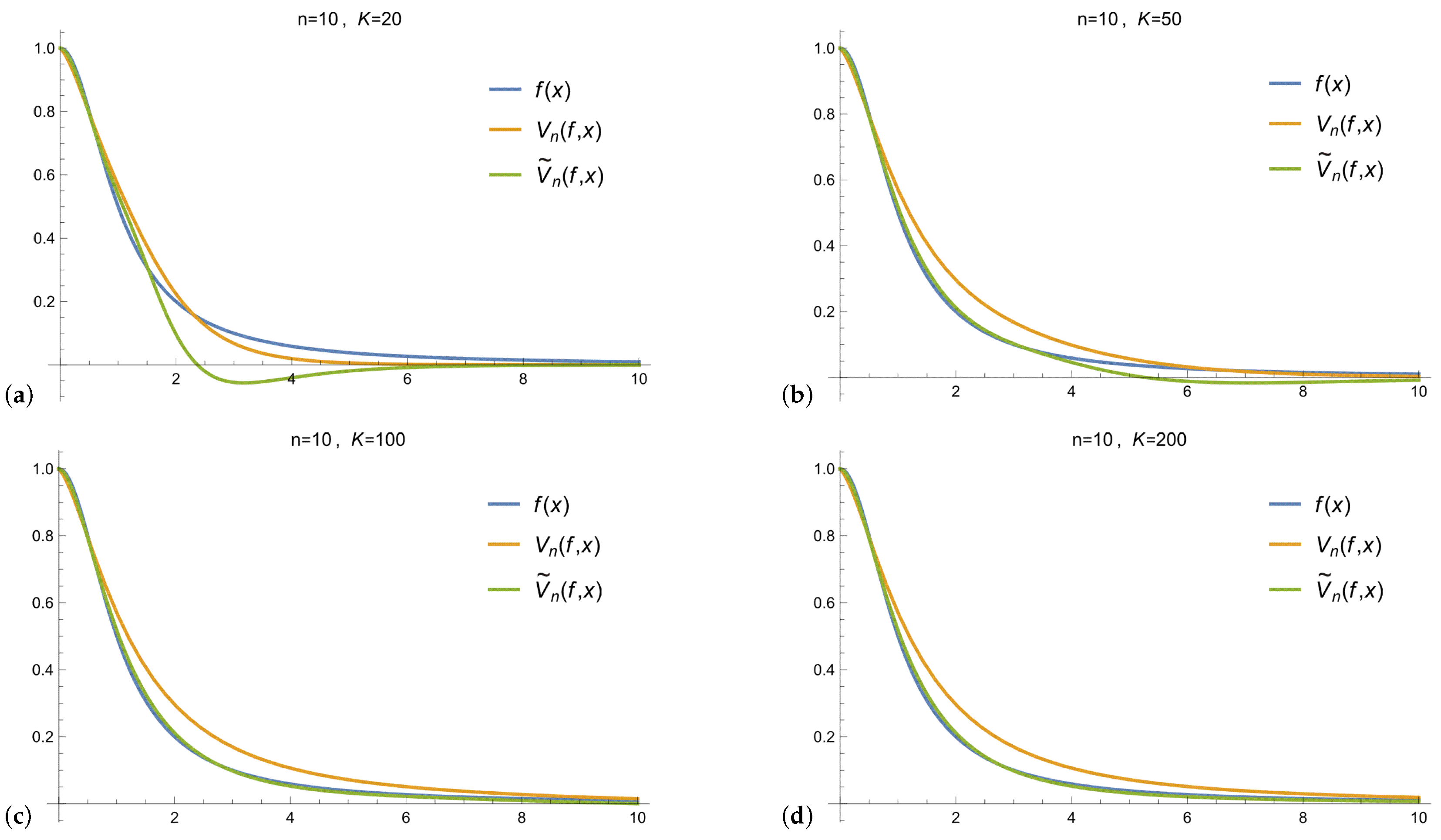
Example 1.

Consider the function $f\left(x\right)={\displaystyle \frac{1}{1+x^2}}$, $x\in [0,\infty )$.

Figure 1 shows graphs of the function $f\left(x\right)$, the Finta operator $V_n(f,x)$, and the operator suggested by the authors ${\tilde{V}}_n(f,x)$ for fixed $n=10$ and both the operators expanded up to order $K=20,50,100,200$. Specifically, on the figure, we present the following approximations of the operators defined in (2) and (4), respectively:

$$V_n(f,x)\approx \sum _{k=0}^K{v}_{n,k}\left(f\right)P_{n,k}\left(x\right)\mathit{and}{\tilde{V}}_n(f,x)\approx \sum _{k=0}^K{v}_{n,k}\left(f\right){\tilde{P}}_{n,k}\left(x\right).$$

Figure 1. Graphs of the function $f\left(x\right)={\displaystyle \frac{1}{1+x^2}}$, the Finta operator $V_n(f,x)$, and the operator ${\tilde{V}}_n(f,x)$ for $n=10$. Panel (a) the case $K=20$; (b) the case $K=50$; (c) the case $K=100$; (d) the case $K=200$.

Absolute error graphs of the above approximations, $|f\left(x\right)-V_n(f,x)|$ and $|f\left(x\right)-{\tilde{V}}_n(f,x)|$, $x\in [0,10]$ are given in Figure 2:

Figure 2. Graphs of the error functions $|f\left(x\right)-V_n(f,x)|$ and $|f\left(x\right)-{\tilde{V}}_n(f,x)|$ for $n=10$. Panel (a) the case $K=20$; (b) the case $K=50$; (c) the case $K=100$; (d) the case $K=200$.

The behavior of the operator ${\tilde{V}}_{n}f$ is much better than $V_{n}f$ for large K.

In the following example, we fix $K=250$ and vary the parameter $n=10,20,30,40$.

Example 2.

Let

$$g\left(x\right)={\displaystyle \frac{e^{-7x^2+4x+5}}{80}}+arctan(x+1)-{\displaystyle \frac{\pi }{2}}.$$

In Figure 3, we show graphs of the function $g\left(x\right)$ and the of operator ${\tilde{V}}_n(g,x)$, $x\in [0,5]$, for fixed $K=250$ and $n=10,20,30,40$.

Figure 3. Graphs of the function $g\left(x\right)={\displaystyle \frac{e^{-7x^2+4x+5}}{80}}+arctan(x+1)-{\displaystyle \frac{\pi }{2}}$ and the operator ${\tilde{V}}_n(g,x)$ for $K=250$. Panel (a) the case $n=10$; (b) the case $n=20$; (c) the case $n=30$; (d) the case $n=40$.

The numerical results confirm the convergence of ${\tilde{V}}_{n}g$ to g as n increases and K is sufficiently large.

6. Conclusions

Our study is in the field of Approximation Theory and the main goal is to suggest a new operator with better approximation properties than the usual Baskakov and Finta operators. Moreover, in order to characterize the approximation error for a family of operators a hard task is to determine the precise quantity to obtain two-sided estimates of the same order. Often the use of appropriate K-functionals helps. While direct results can be obtained, e.g., in terms of moduli of continuity/smoothness or by using Taylor expansion, proving (strong) converse inequalities is much more difficult.

The potential applications to solving differential equations and in CAGD are not the subject of the paper. Of course, one could potentially develop a follow-up paper. However, the authors’ opinion is that there are many problems to overcome from a computational point of view, since (approximate) evaluation of the suggested operator at a point needs numerical computation of sufficiently many improper integrals over the half-line.

The computer simulations show very good behavior of the approximation ${\tilde{V}}_{n}f\approx f$. Although the source code of the algorithms we have implemented comprises just a few lines, the algorithms are of high complexity since they are based on using Wolfram Mathematica functions and adaptive procedures for numerical integration.

In conclusion, the main achievements of our research are theoretical results—extending certain classical inequalities in Approximation Theory to a new operator and settings.