Modeling the Tripodal Mobile Market Using Response Functions Instead of Payoff Maximization

Abstract

We investigate the dynamics of tripodal markets using the response functions, which is a continuation of recent research in the field. Instead of investigating the optimization problem of finding the levels of production that maximize the payoff functions of the participants in an oligopolistic market, based on the available statistical data on market presence, we construct a model of the reaction of the participants. This approach allows, in the absence of information about the cost functions of producers and the demand and utility functions of consumers, to construct a model that is statistically reliable and answers the questions about the levels at which the market has reached equilibrium and whether it is sustainable. On the other hand, any external impact, such as changes in the regulations or the behavior of small market participants, is implicitly included in the response functions. The additional analysis confirms that there are no dependencies, even of a nonlinear type, in the constructed models that are not included. Stability and equilibrium are investigated in the proposed models. The statistical performance measurements for the constructed models are calculated, and their credibility is tested. The models demonstrate high statistical performance and adequacy.

1. Introduction

Modern markets are characterized by the existence of fewer actors who control a large portion of the market. In recent years, there has been considerable study on oligopolistic market places [1,2,3]. The research primarily uses the Cournot model [4] for payoff maximization. As described in the articles, the conventional profit maximization model has constraints [5,6,7]. These can be described as extra demands for differentiability of the profit function, concavity conditions, or second-order conditions implying second-order differentiability. Even if these constraints do not considerably limit the analyzed models, the assumption of rational market players has certain downsides. One such disadvantage is the incorrectness of the pricing function of the items supplied, which results in a model different from the actual one and solutions that are not consistent with rational conduct. Another downside is that participants may be constrained by long-term contracts or technological limitations, which prevent them from making significant adjustments in production volumes, leading to illogical behavior. Despite everything that has been said thus far, in an oligopoly market, all participants have a clear understanding of what changes in the quantities of produced goods they can make, and by knowing their own market results as well as those of the competition—quantities, prices, marketing—they can adjust their policy to the current market situation. This leads to the so-called reaction functions [5,8] of each. These functions rely on the market conditions to determine the modifications each participant should make. A series of studies [5,6,7,9] has shown that in an oligopolistic market with rationally behaving participants and differentiable profit functions, the equilibrium problem approached through reaction functions or the Cournot method gives consistent results for the existence and levels of equilibrium.

The rest of this paper is organized as follows. In Section 2 (Preliminaries), we provide known results about tripled fixed points and market equilibrium in oligopoly, specifically tripodal markets obtained by maximization of the payoff function. We present the connection between tripled fixed points, response functions, and market equilibrium without maximization of the payoff functions. Section 3 (Materials and Methods) provides all necessary definitions and theorems from tripled fixed point theory. Finally, we recall in this section the notions from statistics and modeling: testing the stationarity of time series data; the least squares method; and statistical measures for model estimation. The main findings are in Section 4, which includes a diagram of the available data. We present a sequence of statistical calculations: unit root tests of the initial time series; the unit root test of the differenced time series (Dickey–Fuller F test, Phillips–Perron F test, KPSS test); partial autocorrelation functions (PACFs); Pearson correlation coefficients; and ARIMAX models for the group of firms. The investigated model has a specific feature, namely, two of the operators merge in the considered interval. Consequently, we analyze the market presented either by the three biggest firms or by considering the data of the two merged operators as the data of a single player. All calculations conform a connection in the market shares of the considered mobile providers. Thus, we search for a model based on linear response functions for the three operators Verizon, AT&T, and T-Mobile; a nonlinear model for the operators Verizon, AT&T, and T-Mobile Plus Sprint with moving averages data; and Sigmoidal Models for the three operators. A statistical performance of the created models is presented. We conclude with a discussion in Section 5 (Conclusions).

2. Preliminaries

We present the necessary definitions, notations, and results in two parts: mathematical results and a model of an oligopoly market with three players.

2.1. Fixed Points for Ordered Triples of Maps

The Banach fixed point concept [10], despite being over 100 years old, has numerous extensions and implementations. The generalizations can be classified in different ways. We are only interested in the recommended generalization [11], which alters the concept of fixed points. Coupled fixed points, introduced in [11], are significant in this context.

By considering a map of two variables $F:A\times A\to A$ [11,12], the notion of a coupled fixed point $(x,y)\in A\times A$ of F in A is defined as $x=F(x,y)$ and $y=F(y,x)$.

The concept of exploring fixed points for their existence and uniqueness in cyclic maps, i.e., $T:A\to B$ and $T:B\to A$, versus self-maps was initially presented in [13].

By combining the ideas of cyclic maps and coupled fixed points, the meaning of fixed points was broadened to coupled fixed points for cyclic maps of two variables in [14] by investigating maps $F:A\times A\to A$, $F:B\times B\to A$, and the search for sufficient conditions that will ensure the existence of an ordered pair $(x,y)$ so that $x=F(x,y)$ and $y=F(y,x)$.

However, the equations $x=F(x,y)$ and $y=F(y,x)$ that define the linked fixed points [11,12] frequently result in an ordered pair $(x,y)$ such that $x=y$. This limitation was solved in [15], wherein a modified coupled fixed point for an ordered pair of maps $(F,G)$ was developed. Ref. [15] suggested combining two mappings $F:A\times A\to A$, $G:A\times A\to A$ and defining an ordered pair $(x,y)$ as a coupled fixed point for $(F,G)$ if $x=F(x,y)$ and $y=G(x,y)$. The definition from [11,12] is obtained when $G(x,y)=F(y,x)$.

According to [11], it was suggested to seek an ordered triple $(x,y,z)$ fulfilling $x=F(x,y,z)$, $y=F(y,x,y)$, and $z=F(z,y,x)$, [16]. In [7], generalizations based on the aforementioned were presented, i.e., $x=F(x,y,z)$, $y=G(x,y,z)$, and $z=H(x,y,z)$ for $F,G,H:A^3\to A$. The concept of a tripled fixed point extends to tripled points for ordered triples of maps $(F,G,H)$ that meet the contractive type condition. We will use a simplified version of the main results from [7].

2.2. A Model of an Oligopoly Market Based on Response Functions

Ref. [4] presented an analysis of oligopoly marketplaces, which are dominated by a few major producers who control the price and quantity of goods exchanged. Although the study in [4] used a very simplified model, it has served as a foundational basis for various studies over a century.

In Cournot’s model, a maximization of the payoff functions

$${\Pi }_i(x_1,x_2,\dots ,x_n)=x_{i}P\left(\sum _{i=1}^n{x}_i\right)-c_i\left(x_i\right),i=1,2,\dots ,n$$

for each of the producers is considered, assuming that all of them act rationally (i.e., focus solely on maximizing profit), the price functions P and the cost functions $c_i$, $i=1,2,\dots ,n$ are differentiable. This leads to a system of first-order equations ${\displaystyle \frac{\partial {\Pi }_i}{\partial x_i}}(x_1,x_2,\dots ,x_n)=0$. The first-order equations are only a necessary condition. For these equations, a sufficient condition is required to maximize the payoff functions and thus represent an equilibrium point in the market. These conditions can be either the assumption of the concavity of each ${\Pi }_i$ or the satisfaction of second-order conditions ${\displaystyle \frac{{\partial }^2{\Pi }_i}{\partial x_i^2}}(x_1,x_2,\dots ,x_n)<0$ for each $i=1,2,\dots ,n$.

We will investigate an oligopoly market with three players. In this scenario, the technique of the Cournot model is of gaining $x_1=b_1(x_2,x_3)$, $x_2=b_2(x_1,x_3)$, and $x_3=b_2(x_1,x_2)$, known as response functions [8]. Unfortunately, we may encounter significant technical limitations. It may be challenging or even impossible to find solutions to the system of first-order equations. Even if approximate solutions are identified but the model is unstable, the estimate could be far from the market equilibrium. Using the available statistical data on market presence, we build a model of the participants’ reaction rather than examining the optimization problem of determining the production levels that maximize the payoff functions of the participants in an oligopolistic market [5,7]. This method makes it possible to build a statistically sound model that addresses the issues of whether the market is sustainable and at what point it has reached equilibrium, even in the absence of data regarding the cost functions of producers and the demand and utility functions of consumers. However, the reaction functions implicitly take into account any external influence, such as modifications to laws or the actions of minor market players.

Refs. [5,7] pioneer a different method by discovering an implicit formula for the response functions

$$x_i={\displaystyle \frac{\partial {\Pi }_i}{\partial x_i}}(x_1,x_2,\dots ,x_n)+x_i=F_i(x_1,x_2,x_3),i=1,2,3.$$

It is shown in [5,6] that in an oligopoly market, producers may not always seek to maximize their profit due to different restrictions as extensively commented on in those references. However, they will inevitably respond to the behavior of the other players and the market. It is proven in [6] that whenever the response functions arise from the system of the first-order equations and $F_i$ share some additional conditions, then the second-order conditions are satisfied. Thus, the Cournot model is a particular case of the model of market equilibrium obtained through response functions.

The basic structure suggested in [5,7] is as follows: for each ordered triple of sold production $(x_1,x_2,x_3)$, where $x_i$ is the quantity sold by the $i^{th}$, the $i^{th}$ supplier selects a new level of production $y_i$ based on their technological capabilities and market strategy. Thus, in a subsequent time period, the $i^{th}$ player will generate $y_i=F_i(x_1,x_2,x_3)$. We are looking for a triple $x=(x_1,x_2,x_3)$ of productions that will not affect any of the players’ productions, i.e., $x_i=F(x_1,x_2,x_3)$.

Using the response function transforms the maximization of the payoff functions into a tripled fixed point problem, bypassing all assumptions of concavity and, differentiability [5,6,7].

3. Materials and Methods

3.1. Tripled Fixed Points

We will recall the necessary definitions from [7].

Definition 1 

([7]). Let $I_i$, $i=1,2,3$ be nonempty sets. We will call the ordered triple of maps $(F_1,F_2,F_3)$ a semi-cyclic map if $F_i:I_1\times I_2\times I_3\to I_i$ for $i=1,2,3$.

Definition 2 

([7]). Let $I_i$, $i=1,2,3$ be nonempty sets and the ordered triple $(F_1,F_2,F_3)$ be a semi-cyclic map. An ordered triple $({\xi }_1,{\xi }_2,{\xi }_3)\in I_1\times I_2\times I_3$ is said to be a tripled fixed point of $(F_1,F_2,F_3)$ if ${\xi }_i=F_i({\xi }_1,{\xi }_2,{\xi }_3)$ for $i=1,2,3$.

Definition 3 

([7]). Let $I_i$, $i=1,2,3$ be nonempty sets, and the ordered triple $(F_1,F_2,F_3)$ be a semi-cyclic map. For any triple $\left(x_1^{\left(0\right)},x_2^{\left(0\right)},x_3^{\left(0\right)}\right)\in I_1\times I_2\times I_3$, we define $x_i^{(n+1)}=F_i\left(x_1^{\left(n\right)},x_2^{\left(n\right)},x_2^{\left(n\right)}\right)$, for $i=1,2,3$ for all $n\ge 0$.

3.2. Application in the Study of Market Equilibrium in Tripodal Markets

The following corollary is a simplified version of the primary conclusion from [7], covering the models we will examine.

Corollary 1 

([7]). Let us consider an oligopoly market with three players that satisfies the following conditions:

1.

The three players are producing perfect substitutes of homogeneous products.

2.

The first player can produce quantities from the set $I_1$, and the second and the third ones can produce quantities from the sets $I_2$ and $I_3$, respectively, where $I_1$, $I_2$ and $I_3$ are closed nonempty subsets of a complete metric space $(\mathbb{R},|·|)$.

3.

Let the ordered tripled $(F_1(x,y,z),F_2(x,y,z),F_3(x,y,z))$, $F_i:I_1\times I_2\times I_3\to I_i$, $i=1,2,3$ be a semi-cyclic map that presents the response functions for players one, two, and three, respectively.

4.

Let there be $\alpha <1$ so that the inequality

$$\sum _{i=1}^3|F_i(x_1,x_2,x_3)-F_i(u_1,u_2,u_3)|\le \alpha \sum _{i=1}^3|x_i-u_i|$$

(1)

holds for all $(x_1,x_2,x_3),(u_1,u_2,u_3)\in I_1\times I_2\times I_3$.

Then, there is a unique market equilibrium triple $({\xi }_1,{\xi }_2,{\xi }_3)$ in $I_1\times I_2\times I_3$, i.e., ${\xi }_i=F_i({\xi }_i,{\xi }_2,{\xi }_3)$, for $i=1,2,3$.

1.

Moreover, for any initial start of the market $(x_1^{\left(0\right)},x_2^{\left(0\right)},x_3^{\left(0\right)})\in I_1\times I_2\times I_3$, the sequences $x_i^{(n+1)}=F_i(x_1^{\left(n\right)},x_2^{\left(n\right)},x_2^{\left(n\right)})$, for $i=1,2,3$ converge to $({\xi }_1,{\xi }_2,{\xi }_3)$.

2.

There holds an a priori error estimate

$$\sum _{i=1}^3\left|{\xi }_i-x_i^{\left(n\right)}\right|\le {\displaystyle \frac{{\alpha }^n}{1-\alpha }}\sum _{i=1}^3\left|x_i^{\left(0\right)}-x_i^{\left(1\right)}\right|$$

.

3.

There holds an a posteriori error estimate

$$\sum _{i=1}^3\left|{\xi }_i-x_i^{\left(n\right)}\right|\le {\displaystyle \frac{\alpha }{1-\alpha }}\sum _{i=1}^3\left|x_i^{\left(n\right)}-x_i^{(n-1)}\right|$$

.

4.

The rate of convergence is

$$\sum _{i=1}^3\left|{\xi }_i-x_i^{\left(n\right)}\right|\le \alpha \sum _{i=1}^3\left|{\xi }_i-x_i^{(n-1)}\right|.$$

Additionally, if $F_2(x,y,z)=F_1(y,z,x)$ and $F_3(x,y,z)=F_1(z,x,y)$ are fulfilled, then $\xi =\eta =\zeta$ is satisfied by the market equilibrium triple $(\xi ,\eta ,\zeta )$.

In the event that $F_3(x,y,z)=F_2(x,z,y)$ is also true, $\eta =\zeta$ is satisfied by the market equilibrium triple $(\xi ,\eta ,\zeta )$.

3.3. Sufficient Condition for an Ordered Triple of Semi-Cyclic Maps to Be Contractive

The following proposition is established for two maps f, g of two variables. The proof for three maps with three variables is essentially analogous, so we do not present it here. Proposition 1 provides a sufficient condition for the straightforward application of Corollary 1.

Proposition 1 

([7]). Let $I_i$, $i=1,2,3$ be three intervals in $\mathbb{R}$. Let the functions $f_i:I_1\times I_2\times I_3\to I_i$ have continuous partial derivatives in $I_1\times I_2\times I_3$ such that

$${\displaystyle s_i=sup\left\{\sum _{i=1}^3\left|\frac{\partial f_i}{\partial u_i}(u_1,u_2,u_3)\right|:(u_i,u_2,u_3)\in I_1\times I_2\times I_3\right\}<1,}$$

holds for each $i=1,2,3$.

Then, the ordered pair $(f_1,f_2,f_3)$ satisfies

$$\sum _{i=1}^3|f_i(x_1,x_2,x_3)-f_i(u_1,u_2,u_3)|\le \underset{i=1,2,3}{max}\left\{s_i\right\}\sum _{i=1}^3|x_i-u_i|.$$

3.4. Testing the Stationarity of Time Series Data

In our work, examining the stationarity of time series is essential. A time series is considered stationary when statistical parameters such as mean, variance, covariance, and standard deviation do not change over time. In other words, stationarity implies that there are no trends or seasonal patterns present in the time series. To determine if a time series is stationary, two commonly employed statistical tests are the augmented Dickey–Fuller (ADF) test and the Phillips–Perron (PP) test [17]. Kwiatkowski [18] provides a straightforward test of the null hypothesis of stationarity against the alternative of a unit root. The conclusions drawn from this test complement those based on the Dickey–Fuller test. For this, they consider a three-component representation of the observed time series $Y_1$, $Y_2$, …, $Y_N$ as the sum of a deterministic time trend, a random walk, and a stationary residual:

$$Y_t=\beta ·t+(r_t+\alpha )+e_t$$

(2)

where $r_t=r_{t-1}+u_t$ is a random walk, the initial value $r_0=\alpha$ serves as an intercept, t is is the time index, and $u_t$ are independent identically distributed $(0,{\sigma }_u^2)$. The null and the alternative hypotheses are formulated as follows: $H_0$: ${\sigma }^2=0$ or $r_t$ is a constant, i.e., $Y_t$ is stationary, or $H_1$: $Y_t$ is a unit root process.

An essential aspect of this study is to establish the dependence of the dynamic system at time t on its state at time $t-1$. The partial autocorrelation function (PACF) is a fundamental tool in the time series analysis. PACF [19] measures the direct correlation between time series values at a specific lag, eliminating the effects of all shorter lags. In the present study, the Box–Jenkins ARIMA $(p,d,q)$ methodology [19] is applied for time series analysis. The parameter p indicates the number of lags used in the autoregressive (AR) part of the model, d denotes the degree of differentiation needed to achieve a stationary time series, and q describes the moving average (MA) process, which indicates how many terms are used in the model to smooth out small fluctuations.

3.5. The Least Squares Method

In the present study, we use the famous Least Squares Method (LSM) created by Carl Friedrich Gauss in 1795 and first published by Adrien-Marie Legendre [20]. We implement the LSM by imposing additional constraints on the unknown coefficients described in [9].

3.6. Statistical Measures for Model Estimation

To evaluate the performance of the constructed models, we use two fundamental statistical measures, the coefficient of determination $R^2$ and the mean absolute percentage error (MAPE), which may be calculated using the following formulas:

$${\displaystyle R^2=1-\frac{{\displaystyle \sum _{t=1}^n{(P_t-Y_t)}^2}}{{\displaystyle \sum _{t=1}^n{(Y_t-\overline{Y})}^2}},MAPE=\frac{1}{N}\sum _{t=1}^n\left|\frac{P_t-Y_t}{Y_t}\right|,}$$

(3)

where the sample size is n, the predicted values are $P_t$, the mean is $\overline{Y}$, and the values of the dependent variable are $Y_t$. $R^2$ indicates how well the model explains the variation in the data, and MAPE measures the average forecasting error as a percentage, providing a clear indication of the model’s accuracy.

We aim to generalize the proposed concepts of tripled fixed points so that the obtained results can be applied to the study of market equilibrium, particularly in markets dominated by three producers. Using the statistical techniques discussed, we construct response function models based on real data and examine these real markets for signs of equilibrium and stability.

4. Main Result

Most economic studies aim to identify the factors influencing competitiveness, economic success, predicting consumer behavior, and forecasting demand and sales. High-performance statistical models are constructed via classical or machine learning methods, such as panel regression, multiple linear regression, principal component analysis, and Box–Jenkins ARIMA methodology [21,22]. The authors [23] effectively utilize powerful machine learning methods with high predictive capabilities such as convolutional neural networks, the long short-term memory network, and ensemble methods. However, the current investigation does not focus on building a high-performance statistical model of real data for prediction purposes. Instead, we are seeking a sufficiently appropriate statistical model that aligns with the constraints of Corollary 1 to analyze the equilibrium point.

We will use response functions to study the US mobile market from 2011 to 2023. In [9], a market inquiry is conducted between 2011 and 2020, utilizing the suggested response function technique. The merger of T-Mobile and Sprint in 2020 complicates the evaluation of a tripodal market in [9]. Recent statistics indicate that the duopoly market of AT&T and Verizon has grown into a tripodal market controlled by AT&T, Verizon, and T-Mobile. We will propose several hypotheses based on statistical data and present several modeling ideas. We will create models distinguishing T-Mobile customers for over the entire period or combine T-Mobile and Sprint consumers throughout. We will build linear, nonlinear, and sigmoidal response functions. Following [7], which demonstrates the benefits of smoothing data with moving averages, we will model linear, nonlinear, and sigmoidal response functions. Our models will be based on moving average data rather than real data.

4.1. Empirical Data

In our research, we use quarterly data on mobile provider shares in the US, expressed in percentages, from Q1-2011 to Q3-2023. Figure 1 shows the market shares of the four important mobile carriers.

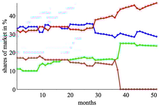
Figure 1. Market share percentages for Verizon (blue), AT&T (red), T-Mobile (green), and Sprint (brown).

Let us add that in Q3-2020, the mobile providers T-Mobile and Sprint merged, leading to Sprint’s withdrawal from the market and a subsequent shift of its customers to T-mobile. Thus, there was a substantial increase in T-Mobile’s market shares.

This is the reason why we consider a market dominated by only three large mobile service providers. Figure 1 is included only to illustrate how the fourth operator disappears from the market. It would not be possible to study the market assuming four providers because, for the last four years, the fourth one (Sprint) has had a market share of $0\%$. In what follows, we assume two scenarios for the 2011–2020 interval: (1) T-Mobile has only its market share, or (2) T-Mobile includes its users and those of Sprint combined. The analyses will show that both assumptions are statistically reliable.

For simplicity, we designate each mobile provider with a variable in parentheses: Verizon ($Mo{b}_1$), AT&T ($Mo{b}_2$), T-Mobile ($Mo{b}_3$), T-Mobile, and Sprint ($Mo{b}_4$).

Table 1 displays the results of the unit root tests conducted on the original time series. Since all p-values for the starting variables are negligible, the time series has a first-order trend and is non-stationary.

Table 1. Result from the unit root tests of the initial time series.

Statistics		${\mathit{Mob}}_{\mathbf{1}}$	${\mathit{Mob}}_2$	${\mathit{Mob}}_3$	${\mathit{Mob}}_4$
Dickey–Fuller F test	statistic	−0.165	0.400	0.549	−0.182
	p-value	0.642	0.782	0.817	0.638
Phillips–Perron F test	statistic	−0.161	0.402	0.548	−0.175
	p-value	0.643	0.782	0.817	0.639

For the differenced series $\Delta Mo{b}_i,i=1,\dots ,4$ calculated by

$$\Delta Y_t=Y_t-Y_{t-1},$$

(4)

Table 2 provides the corresponding unit root test indices. Since all of the p-values in this table are essentially zero, the unit root problem is resolved. It is presumed that the difference variables are stationary.

Table 2. Outcomes of the unit root test of the differenced time series.

Statistics		$\mathbf{\Delta }{\mathit{Mob}}_1$	$\mathbf{\Delta }{\mathit{Mob}}_2$	$\mathbf{\Delta }{\mathit{Mob}}_3$	$\mathbf{\Delta }{\mathit{Mob}}_4$
Dickey–Fuller F test	statistic	−47.65	−45.41	−44.71	−44.71
	p-value	$2.42·{10}^{-7}$	$3.79·{10}^{-7}$	$4.37·{10}^{-7}$	$4.37·{10}^{-7}$
Phillips–Perron F test	statistic	−43.72	−41.92	−42.08	−42.08
	p-value	$9.83·{10}^{-8}$	$7.93·{10}^{-7}$	$7.65·{10}^{-7}$	$7.65·{10}^{-7}$

The unit root tests confirm the presence or first-order trends in all variables. This basically means that the time series values for each month may be represented in terms of the previous month’s data. Table 3 presents the KPSS test values for the four variables. The significant p-values indicate that the time series are not stationary around the mean, suggesting that the average level of the series changes over time. In cases where the trend of the series is not clearly defined, this may be due to strong fluctuations or changes in the data structure over time. The first three series are not stationary around the mean at the 1% significance level, while the fourth series, $Mo{b}_4$, is non-stationary at the 5% significance level.

Table 3. Outcomes of the unit root test of the differenced time series.

Statistics		${\mathit{Mob}}_1$	${\mathit{Mob}}_2$	${\mathit{Mob}}_3$	${\mathit{Mob}}_4$
KPSS test	statistic	0.7398	0.9977	0.9695	0.5436
	p-value	0.01	0.01	0.01	0.032
	Critical Values	1%:0.739	1%:0.739	1%:0.739	5%:0.463

Figure 2 and Figure 3 show the partial autocorrelation functions (PACFs) of the four mobile operators.

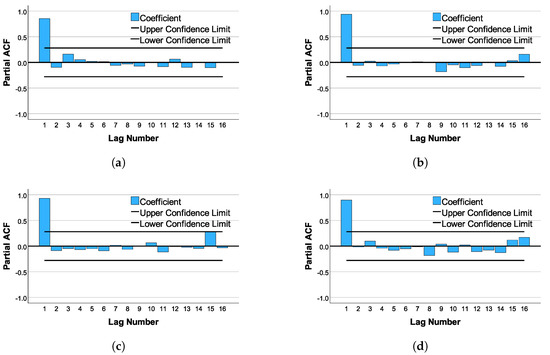
Figure 2. PACF of the initial time series. (a) PACF of the initial time series $Mo{b}_1$; (b) PACF of the initial time series of $Mo{b}_2$; (c) PACF of the initial time series of $Mo{b}_3$; (d) PACF of the initial time series of $Mo{b}_4$.

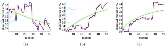
Figure 3. An approximation by using the ordered triple of response functions $(f_1,f_2,f_3)$. (a) $Mo{b}_1$: blue—the real data, red—an approximation using $u_1^{(n+1)}=f_1\left(u_1^{\left(n\right)},u_2^{\left(n\right)},u_3^{\left(n\right)}\right)$, green—an approximation using $u_1^{(n+1)}=f_1^{n+1}\left(u_1^{\left(0\right)},u_2^{\left(0\right)},u_3^{\left(0\right)}\right)$; (b) $Mo{b}_2$: blue—the real data, red—an approximation using $u_2^{(n+1)}=f_2\left(u_1^{\left(n\right)},u_2^{\left(n\right)},u_3^{\left(n\right)}\right)$, green—an approximation using $u_2^{(n+1)}=f_2^{n+1}\left(u_1^{\left(0\right)},u_2^{\left(0\right)},u_3^{\left(0\right)}\right)$; (c) $Mo{b}_3$: blue-the real data, red-an approximation using $u_3^{(n+1)}=f_3\left(u_1^{\left(n\right)},u_2^{\left(n\right)},u_3^{\left(n\right)}\right)$, green—an approximation using $u_3^{(n+1)}=f_3^{n+1}\left(u_1^{\left(0\right)},u_2^{\left(0\right)},u_3^{\left(0\right)}\right)$.

In all four PACF graphs, the first lag is clearly outside the confidence interval, and the autocorrelation function value is close to 1. This indicates that, for each of the examined time series, there is a dependence between consecutive time points. For this reason, we examine the time series data lagged by one period and investigate the correlation dependencies among all variables. The Pearson correlation coefficient (PCC) and their two-tailed significance values (Sig.) are shown in Table 4.

Table 4. Pearson correlation coefficients.

		${\mathit{Mob}}_1$	${\mathit{Mob}}_2$	${\mathit{Mob}}_3$	${\mathit{Mob}}_4$	Lag ${\mathit{Mob}}_1$	Lag ${\mathit{Mob}}_2$	Lag ${\mathit{Mob}}_3$	Lag ${\mathit{Mob}}_4$
$Mo{b}_1$	PCC	1	−0.852	−0.587	0.481	0.873	−0.820	−0.568	0.507
	Sig.		<0.001	<0.001	<0.001	<0.001	<0.001	<0.001	<0.001
$Mo{b}_2$	PCC		1	0.885	−0.720	−0.825	0.982	0.866	−0.691
	Sig.				<0.001	<0.001	<0.001	<0.001	<0.001
$Mo{b}_3$	PCC			1	−0.596	−0.591	0.888	0.964	−0.574
	Sig.				<0.001	<0.001	<0.001	<0.001	<0.001
$Mo{b}_4$	PCC				1	0.548	−0.735	−0.607	0.923
	Sig.					<0.001	<0.001	<0.001	<0.001
Lag $Mo{b}_1$	PCC					1	−0.845	−0.571	0.455
	Sig.						<0.001	<0.001	<0.001
Lag $Mo{b}_2$	PCC						1	0.882	−0.702
	Sig.							<0.001	<0.001
Lag $Mo{b}_3$	PCC							1	−0.578
	Sig.								<0.001

From Table 4, it can be seen that all correlation coefficients are significant. We should note the strong correlation dependencies between $Mo{b}_1$, $Mo{b}_3$, $Mo{b}_4$, and Lag $Mo{b}_2$, that is, from the indicators of $Mo{b}_2$ in the previous quartile. We also observe a strong correlation between $Mo{b}_2$ and Lag $Mo{b}_3$.

In this study, ARIMA models with transfer functions (ARIMAX) are constructed for each time series, with the remaining time series used as predictors. Two groups of time series are examined: $Mo{b}_1$, $Mo{b}_2$, $Mo{b}_3$, and $Mo{b}_1$, $Mo{b}_2$, and $Mo{b}_4$. The models are identified and estimated in accordance with the Box–Jenkins methodology. The corresponding ARIMAX models for the group $Mo{b}_1$, $Mo{b}_2$, and $Mo{b}_3$ are presented in Table 5.

Table 5. ARIMAX models for the group $Mo{b}_1$, $Mo{b}_2$, and $Mo{b}_3$.

$\mathit{Dependent}$	${\mathit{Independent}}_1$	${\mathit{Independent}}_2$	Model	${\mathit{R}}^2$	$\mathit{MAPE}$	p-Value (Ljung–Box Test)	Remarks
$Mo{b}_1$	$Mo{b}_2$	$Mo{b}_3$	ARIMA(0,1,0)(0,0,0)	0.832	1.702	0.959	$Mo{b}_2$ (diff.=1); $Mo{b}_3$ (insign.)
$Mo{b}_2$	$Mo{b}_1$	$Mo{b}_3$	ARIMA(0,1,0)(1,1,0)	0.971	1.621	0.554	$Mo{b}_1$ (diff.=1, season.diff.=1); $Mo{b}_3$ (diff.=1)
$Mo{b}_3$	$Mo{b}_1$	$Mo{b}_2$	ARIMA(0,1,0)(0,0,0)	0.949	3.781	0.926	natural log. transf., $Mo{b}_1$ (diff.=1); $Mo{b}_2$ (diff.=1, lag=1)

For the group $Mo{b}_1$, $Mo{b}_2$, $Mo{b}_4$, the corresponding ARIMAX models are given in Table 6.

Table 6. ARIMAX models for group $Mo{b}_1$, $Mo{b}_2$, and $Mo{b}_4$.

$\mathit{Dependent}$	${\mathit{Independent}}_1$	${\mathit{Independent}}_2$	Model	${\mathit{R}}^2$	$\mathit{MAPE}$	p-Value (Ljung–Box Test)	Remarks
$Mo{b}_1$	$Mo{b}_2$	$Mo{b}_4$	ARIMA(0,1,0)(0,0,0)	0.928	1.017	0.811	$Mo{b}_2$ (diff.=1); $Mo{b}_4$ (diff.=1)
$Mo{b}_2$	$Mo{b}_1$	$Mo{b}_4$	ARIMA(0,1,0)(0,1,0)	0.987	1.055	0.705	$Mo{b}_1$ (diff.=1, season.diff.=1); $Mo{b}_4$ (diff.=1, season.diff.=1)
$Mo{b}_4$	$Mo{b}_1$	$Mo{b}_2$	ARIMA(0,1,0)(0,0,0)	0.937	1.345	0.809	natural log. transf., $Mo{b}_1$ (diff.=1); $Mo{b}_2$ (diff.=1)

The constructed models explain over $83\%$ of the variation in the data and show no significant autocorrelation in the residuals (based on the Ljung–Box tests) and ACF. These models exhibit very good statistical performance—high coefficients of determination and low errors (MAPE). The primary role of these models is to demonstrate the dependence of each time series at a given moment on the state of the system from the previous time point. As seen from the constructed models, first-order differencing, i.e., $\Delta Y_t=Y_t-Y_{t-1}$, is included in each model, indicating that the previous period’s influence is essential for the time series considered as a whole.

4.2. Modeling the Response Functions of the Three Producers

We have genuine statistics on the quantities sold for 51 consecutive quarters. The responses of the two biggest providers Verizon and AT&T are investigated in [9]. The analysis in [9] suggests that the response function should be of a sigmoidal type. At the time of the above-mentioned investigation [9], the merger between T-Mobile and Sprint had just occurred and therefore there were not sufficient data to analyze an oligopoly market with three main players.

In this section, we present several possible market response models and use the notation from the ”Materials and Methods” section. Let $x_1^{\left(n\right)}$, $x_2^{\left(n\right)}$, and $x_3^{\left(n\right)}$ represent the percentage shares of the three mobile providers $Mo{b}_1$, $Mo{b}_2$, and $Mo{b}_3$, respectively, during the quarter $n=1,2,\dots ,51$.

Following [7], we will search for functions $f_i(x,y,z)$, $i=1,2,3$, where $f_i$ is the response function of $Mo{b}_i$ such that

$$f_i\left(x_1^{\left(n\right)},x_2^{\left(n\right)},x_3^{\left(n\right)}\right)=f_i\left(x_1^{(n-1)},x_2^{(n-1)},x_3^{(n-1)}\right)fori=1,2,3andn=2,3,\dots ,51,$$

(5)

to solve the minimizing problem

$${\displaystyle \sum _{k=2}^{51}\left(\sum _{i=1}^3{\left(x_i^{\left(k\right)}-f_i(x_1^{(k-1)},x_2^{(k-1)},x_3^{(k-1)}\right)}^2\right)\to min.}$$

(6)

4.3. A Model Based on Linear Response Functions for the Three Operators Verizon, AT&T, and T-Mobile

We are looking for response functions within the form

$$f_i\left(x_1,x_2,x_3\right)=\sum _{j=1}^3{a}_{ij}{x}_j+d_i$$

for $i=1,2,3$.

Let us denote

$${\eta }_i^{\left(n\right)}=\sum _{j=1}^3{a}_{ij}{x}_j^{(n-1)}+a_{i2}{x}_2^{(n-1)}+a_{i3}{x}_3^{(n-1)}+d_i=f_i\left(x_1^{(n-1)},x_2^{(n-1)},x_3^{(n-1)}\right),$$

(7)

for $i=1,2,3$.

The coefficients $a_{ij},d_i\in \mathbb{R}$, $i,j=1,2,3$ are determined by minimizing the sum of the squares of the differences

$${\displaystyle \sum _{k=2}^{51}\left(\sum _{i=1}^3{\left(x_i^{\left(k\right)}-{\eta }_i^{\left(k\right)}\right)}^2\right)\to min,}$$

(8)

subject to constraints based on the model, Corollary 1, and the observations made in [7,9].

Thus, we obtain the response functions

$$\left\{\begin{array}{cccccc}{f}_1(x,y,z)\hfill & =& \hfill 0.71x& \hfill -0.1y& \hfill +0.006z& \hfill +12.85,\\ f_2(x,y,z)\hfill & =& \hfill -0.16x& \hfill +0.84y& \hfill +0.09z& \hfill +9.48,\\ f_3(x,y,z)\hfill & =& \hfill -0.04x& \hfill +0.04y& \hfill +0.88z& \hfill +2.04.\end{array}\right.$$

(9)

Putting

$$s_i=sup\left\{\sum _{i=1}^3\left|{\displaystyle \frac{\partial f_i}{\partial u_1}}(u_1,u_2,u_3)\right|:u_i\in I_i,i=1,2,3\right\}$$

we calculate $s_1<0.92$, $s_2<0.89$, and $s_3<0.98$. By Proposition 1, we conclude that we can apply Corollary 1.

Assuming the three mobile providers follow the response functions $f_i$ for $i=1,2,3$, a market equilibrium exists. For any initial state in the market, successive iterations will converge to the unique market equilibrium points $({\xi }_1,{\xi }_2,{\xi }_3)$. We identify that the market equilibrium is the solution to the system of equations:

$$f_i({\xi }_1,{\xi }_2,{\xi }_3)={\xi }_i,fori=1,2,3,$$

e.g., $({\xi }_1,{\xi }_2,{\xi }_3)=(28.6,46.9,23.5)$.

Figure 3 illustrates the market shares of the three mobile operators over time as approximated by the response functions $f_i$, $i=1,2,3$. The blue color represents the actual data, the red color indicates approximated values from the previous quarter, and the green color shows iterated estimates based on the market’s first quartile.

Table 7 shows the high statistical indicators of the constructed models with a coefficient of determination above 98% and MAPE below 2%. The ACF (autocorrelation function) plots in Figure 4 display autocorrelations of the residuals at different lags for the built models. Most of the bars (representing the autocorrelation coefficients) fall within the confidence bounds (indicated by the two black lines), which suggests that there is no significant autocorrelation at the shown lags. The absence of significant spikes indicates that the residuals behave like white noise, implying that the models adequately capture the autocorrelation structure in the data.

Table 7. Statistical performance of the created models.

	Model ${\mathit{Mob}}_1$	Model ${\mathit{Mob}}_2$	Model ${\mathit{Mob}}_3$
$R^2$	0.985	0.999	0.998
MAPE	0.00962	0.00789	0.02305

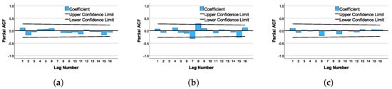
Figure 4. ACF plots of the residuals in the models. (a) ACF plot of the residuals in the model for $Mo{b}_1$; (b) ACF plot of the residuals in the model for $Mo{b}_2$; (c) ACF plot of the residuals in the model for $Mo{b}_3$.

The Ljung–Box test [19,24] for autocorrelation and the Brock–Dechert–Scheinkman (BDS) test [25] for nonlinearity are both conducted on the models’ residuals. The p-values for both tests are insignificant for the three models, indicating that the residuals are approximately independent and identically distributed (i.i.d.), which suggests that the model provides an adequate fit to the data.

Similar results are observed for the residuals of the next three investigated models, which we will not elaborate on, as the calculations are essentially the same. Therefore, the proposed four models provide an adequate data fit.

4.4. The Nonlinear Model for the Operators Verizon, AT&T, and T-Mobile plus Sprint with Moving Averages Data

The merger of T-Mobile and Sprint leads to the feasible assumption that their clients can be grouped together in the model for all 51 quartiles. Figure 5a depicts percentage shares over time for Verizon (blue), AT&T (red), and T-Mobile plus Sprint (green). Figure 5a demonstrates that the graph of T-Mobile plus Sprint does not exhibit linear behavior. Ref. [7] suggests using moving averages to smooth the data and eliminate oscillations from the actual data; see Figure 5b.

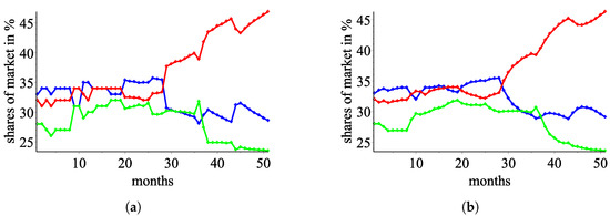
Figure 5. (a,b) Market share percentages over time for Verizon (blue), AT&T (red), and T-Mobile + Sprint (green).

Following the remarks in [7], it appears logical to smooth the real data using weighted moving average data.

Figure 5 recommends investigating the response function for T-Mobile and Sprint in the form

$$g_3(x_1,x_2,x_3)=\sum _{i=1}^3{a}_{3i}{x}_i+e_3{x}_3^2+d_3$$

and

$$g_k(x_1,x_2,x_3)=\sum _{i=1}^3{a}_{k1}{x}_i+d_k$$

for Verizon and AT&T, respectively.

Thus, we calculate

$${\eta }_i^{\left(n\right)}=g_i\left(x_1^{(n-1)},x_2^{(n-1)},x_3^{(n-1)}\right).$$

(10)

The coefficients $a_{ij},d_i,e_3\in \mathbb{R}$, $i,j=1,2,3$ are determined by minimizing the sum of the squares of the differences

$${\displaystyle \sum _{k=2}^{51}\left(\sum _{i=1}^3{\left(x_i^{\left(k\right)}-{\eta }_i^{\left(k\right)}\right)}^2\right)\to min,}$$

(11)

subject to some additional constraints.

Thus, we obtain the response functions

$$\left\{\begin{array}{ccccc}{g}_1(x,y,z)\hfill & =& 0.89x-\hfill & \hfill 0.02y& +0.03z+2.91,\hfill \\ g_2(x,y,z)\hfill & =& 0.03x+\hfill & \hfill 0.97y& +0.01z+2.06,\hfill \\ g_3(x,y,z)\hfill & =& 0.06x-\hfill & \hfill 0.003y& +0.37z+0.01z^2+7.46.\hfill \end{array}\right.$$

(12)

Setting

$$s_i=sup\left\{\sum _{i=1}^3\left|{\displaystyle \frac{\partial g_i}{\partial u_1}}(u_1,u_2,u_3)\right|:u_i\in I_i,i=1,2,3\right\}$$

we calculate $s_1<0.99$, $s_2<0.99$, and $s_3<0.95$. By Proposition 1, we conclude that we can apply Corollary 1. Assuming the three mobile providers follow the response functions $g_i$ for $i=1,2,3$, a market equilibrium exists. For any initial condition in the market, successive iterations will converge to the unique market equilibrium points $({\xi }_1,{\xi }_2,{\xi }_3)$. We identify that the market equilibrium is the solution to the system of equations

$$g_i({\xi }_1,{\xi }_2,{\xi }_3)={\xi }_i,fori=1,2,3,$$

e.g., $({\xi }_1,{\xi }_2,{\xi }_3)=(28.6,46.9,23.5)$.

Figure 6 depicts the market shares of the three mobile operators over time as approximated by the response functions $g_i$, $i=1,2,3$. The blue color represents actual data, the red color indicates approximated numbers from the previous quarter, and the green color reflects iterated estimates based on the market’s first quartile. The statistical performance is calculated in Table 8.

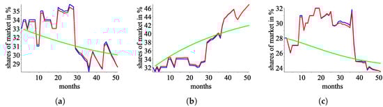
Figure 6. An approximation by using the ordered triple of response functions $(g_1,g_2,g_3)$. (a) $Mo{b}_1$: blue—the real data, red—an approximation using $u_1^{(n+1)}=g_1\left(u_1^{\left(n\right)},u_2^{\left(n\right)},u_3^{\left(n\right)}\right)$, green—an approximation using $u_1^{(n+1)}=g_1^{n+1}\left(u_1^{\left(0\right)},u_2^{\left(0\right)},u_3^{\left(0\right)}\right)$; (b) $Mo{b}_2$: blue—the real data, red—an approximation using $u_2^{(n+1)}=g_2\left(u_1^{\left(n\right)},u_2^{\left(n\right)},u_3^{\left(n\right)}\right)$, green—an approximation using $u_2^{(n+1)}=g_2^{n+1}\left(u_1^{\left(0\right)},u_2^{\left(0\right)},u_3^{\left(0\right)}\right)$; (c) $Mo{b}_4$: blue—the real data, red—an approximation using $u_3^{(n+1)}=g_3\left(u_1^{\left(n\right)},u_2^{\left(n\right)},u_3^{\left(n\right)}\right)$, green—an approximation using $u_3^{(n+1)}=g_3^{n+1}\left(u_1^{\left(0\right)},u_2^{\left(0\right)},u_3^{\left(0\right)}\right)$.

Table 8. Statistical performance of the created models.

	Model ${\mathit{Mob}}_1$	Model ${\mathit{Mob}}_2$	Model ${\mathit{Mob}}_4$
$R^2$	0.8917	0.9848	0.9422
MAPE	0.0192	0.01477	0.0160

4.5. A Sigmoidal Model for the Three Operators Verizon, AT&T, and T-Mobile Modeled on Moving Average Data

Following [9], we shall look for response functions generated using sigmoids, specifically the type of sigmoid functions described in [9]. The response functions are defined as follows:

$$h_1(x_1,x_2,x_3)={\displaystyle \frac{a_1}{e_1+q_1{x}_1}}+s_1{x}_1+{\displaystyle \frac{b_1}{f_1+p_1{x}_2}}+c_1{x}_3+d_1$$

$$h_2(x_1,x_2,x_3)={\displaystyle \frac{a_2}{e_2+q_2{x}_1}}+{\displaystyle \frac{b_2}{f_2+p_2{x}_2}}+s_2{x}_2+c_2{x}_3+d_2$$

$$h_3(x_1,x_2,x_3)=a_3{x}_1+b_3{x}_2+s_3{x}_3+d_3.$$

We will refer to this model as semi-sigmoidal because we insert a linear function $s_i{x}_i$ in the response function $H_i$ for $i=1,2$, respectively, and a linear model for the response of the third provider.

Thus, we calculate

$${\eta }_i^{\left(n\right)}=h_i\left(x_1^{(n-1)},x_2^{(n-1)},x_3^{(n-1)}\right).$$

(13)

After minimizing the sum of the squares of the differences

$${\displaystyle \sum _{k=2}^{51}\left(\sum _{i=1}^3{\left(x_i^{\left(k\right)}-{\eta }_i^{\left(k\right)}\right)}^2\right)\to min,}$$

(14)

subject to some restrictions, we obtain the response functions

$$\left\{\begin{array}{c}{\displaystyle h_1(x_1,x_2,x_3)=\frac{-0.002}{0.92+1.49x_1}+0.89x_1-\frac{0.002}{0.84-2.07x_2}+3.58,}\hfill \\ {\displaystyle h_2(x_1,x_2,x_3)=\frac{0.9}{1.0+1.01x_1}-\frac{0.07}{1.28+2.21x_2}+0.95x_2+0.02x_3+1.79,}\hfill \\ h_3(x_1,x_2,x_3)=-0.06x_1+0.93x_3+3.42.\hfill \end{array}\right.$$

(15)

Let us point out that in this model, the coefficients $c_1$ and $b_3$ are equal to zero.

Setting

$$s_i=sup\left\{\sum _{i=1}^3\left|{\displaystyle \frac{\partial g_i}{\partial u_1}}(u_1,u_2,u_3)\right|:u_i\in I_i,i=1,2,3\right\},$$

we calculate $max\left\{s_i\right\}<0.95$ and by Proposition 1, we conclude that we can apply Corollary 1. Assuming the three mobile providers follow the response functions $h_i$ for $i=1,2,3$, a market equilibrium exists. For any initial condition in the market, successive iterations will converge to the unique market equilibrium points $({\xi }_1,{\xi }_2,{\xi }_3)$. We identify that the market equilibrium is the solution to the system of equations

$$h_i({\xi }_1,{\xi }_2,{\xi }_3)={\xi }_i,fori=1,2,3,$$

e.g., $({\xi }_1,{\xi }_2,{\xi }_3)=(31.6,44.03,21.12)$. Figure 7 presents the behavior over time in the mobile market when modeled by the triple of response functions $(h_1,h_2,h_3)$, and Table 9 gives the statistical performance of the above-mentioned model.

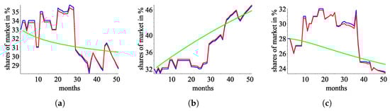
Figure 7. An approximation by using the ordered triple of response functions $(h_1,h_2,h_3)$. (a) $Mo{b}_1$: blue—the real data, red—an approximation using $u_1^{(n+1)}=h_1\left(u_1^{\left(n\right)},u_2^{\left(n\right)},u_3^{\left(n\right)}\right)$, green—an approximation using $u_1^{(n+1)}=h_1^{n+1}\left(u_1^{\left(0\right)},u_2^{\left(0\right)},u_3^{\left(0\right)}\right)$; (b) $Mo{b}_2$: blue—the real data, red—an approximation using $u_2^{(n+1)}=h_2\left(u_1^{\left(n\right)},u_2^{\left(n\right)},u_3^{\left(n\right)}\right)$, green—an approximation using $u_2^{(n+1)}=h_2^{n+1}\left(u_1^{\left(0\right)},u_2^{\left(0\right)},u_3^{\left(0\right)}\right)$; (c) $Mo{b}_4$: blue—the real data, red—an approximation using $u_3^{(n+1)}=h_3\left(u_1^{\left(n\right)},u_2^{\left(n\right)},u_3^{\left(n\right)}\right)$, green—an approximation using $u_3^{(n+1)}=h_3^{n+1}\left(u_1^{\left(0\right)},u_2^{\left(0\right)},u_3^{\left(0\right)}\right)$.

Table 9. Statistical performance of the constructed models.

	Model ${\mathit{Mob}}_1$	Model ${\mathit{Mob}}_2$	Model ${\mathit{Mob}}_3$
$R^2$	0.8945	0.9844	0.9406
MAPE	0.1965	0.01417	0.0157

4.6. A Sigmoidal Model for the Three Operators Verizon, AT&T, and T-Mobile plus Sprint

To conclude the presentations, we provide a model of response functions based on sigmoidal functions derived from real data and the merging of the shares of T-Mobile and Sprint. Based on [9], we assume the two larger suppliers have sigmoidal response functions and do not consider the behavior of minor market participants. Thus, we look for response functions of the following type:

$$S_1(x_1,x_2,x_3)={\displaystyle \frac{a_1}{e_1+q_1{x}_1}}+s_1{x}_1+{\displaystyle \frac{b_1}{f_1+p_1{x}_2}}+d_1$$

$$S_2(x_1,x_2,x_3)={\displaystyle \frac{a_2}{e_2+q_2{x}_1}}+{\displaystyle \frac{b_2}{f_2+p_2{x}_2}}+s_2{x}_2+d_2$$

$$S_3(x_1,x_2,x_3)=a_3{x}_1+b_3{x}_2+s_3{x}_3+d_3$$

In this model, we calculate based on the real data, rather than the smoothed data, while combining the market shares of T-Mobile and Sprint.Thus, we calculate

$${\eta }_i^{\left(n\right)}=S_i\left(x_1^{(n-1)},x_2^{(n-1)},x_3^{(n-1)}\right).$$

(16)

After minimizing the sum of the squares of the differences

$${\displaystyle \sum _{k=2}^{51}\left(\sum _{i=1}^3{\left(x_i^{\left(k\right)}-{\eta }_i^{\left(k\right)}\right)}^2\right)\to min,}$$

(17)

subject to some restrictions, we obtain the following response functions:

$$\left\{\begin{array}{c}{S}_1(x,y,z)=0.87x_1-{\displaystyle \frac{0.000003}{4.38+4.32x_2}}+3.71,\hfill \\ {\displaystyle S_2(x,y,z)=\frac{20.44}{3.55+0.09x_1}+0.92x_2+0.41,}\hfill \\ S_3(x,y,z)=0.15x_2+0.77x_3-1.32.\hfill \end{array}\right.$$

(18)

Let us comment that $a_1=e_1=q_1=b_2=f_2=p_2=a_3=0$.

Setting

$$s_i=sup\left\{\sum _{i=1}^3\left|{\displaystyle \frac{\partial S_i}{\partial u_1}}(u_1,u_2,u_3)\right|:u_i\in I_i,i=1,2,3\right\},$$

we calculate $max\left\{s_i\right\}<0.92$, and by Proposition 1, we conclude that we can apply Corollary 1. Assuming the three mobile providers follow the response functions $S_i$ for $i=1,2,3$, a market equilibrium exists. For any initial condition in the market, successive iterations will converge to the unique market equilibrium points $({\xi }_1,{\xi }_2,{\xi }_3)$. We identify that the market equilibrium is the solution to the system of equations

$$S_i({\xi }_1,{\xi }_2,{\xi }_3)={\xi }_i,fori=1,2,3,$$

e.g., $({\xi }_1,{\xi }_2,{\xi }_3)=(28.6,46.9,23.5)$. Figure 8 presents the behavior over time in the mobile market when modeled by the triple of response functions $(S_1,S_2,S_3)$, and Table 10 gives the statistical performance of the above-mentioned model.

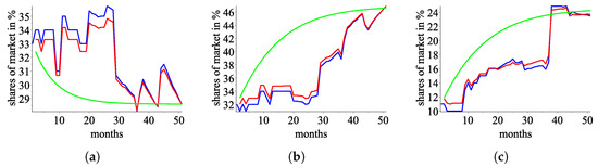
Figure 8. An approximation by using the ordered triple of response functions $(S_1,S_2,S_3)$. (a) $Mo{b}_1$: blue—the real data, red—an approximation using $u_1^{(n+1)}=S_1\left(u_1^{\left(n\right)},u_2^{\left(n\right)},u_3^{\left(n\right)}\right)$, green—an approximation using $u_1^{(n+1)}=S_1^{n+1}\left(u_1^{\left(0\right)},u_2^{\left(0\right)},u_3^{\left(0\right)}\right)$; (b) $Mo{b}_2$: blue—the real data, red—an approximation using $u_2^{(n+1)}=S_2\left(u_1^{\left(n\right)},u_2^{\left(n\right)},u_3^{\left(n\right)}\right)$, green—an approximation using $u_2^{(n+1)}=S_2^{n+1}\left(u_1^{\left(0\right)},u_2^{\left(0\right)},u_3^{\left(0\right)}\right)$; (c) $Mo{b}_3$: blue—the real data, red—an approximation using $u_3^{(n+1)}=S_3\left(u_1^{\left(n\right)},u_2^{\left(n\right)},u_3^{\left(n\right)}\right)$, green—an approximation using $u_3^{(n+1)}=S_3^{n+1}(u_1^{\left(0\right)},u_2^{\left(0\right)},u_3^{\left(0\right)})$.

Table 10. Statistical performance of the created models.

	Model ${\mathit{Mob}}_1$	Model ${\mathit{Mob}}_2$	Model ${\mathit{Mob}}_3$
$R^2$	0.999	0.999	0.993
MAPE	0.0138	0.0178	0.0356

5. Conclusions

A well-known approach for investigating market equilibrium in an oligopoly [4] has undergone development and various extensions. It is based on maximizing the payoff function for a known demand function for the provided products or services. The inability to develop and investigate the demand function is a key shortcoming of the [4] approach, making it more suitable for theoretical research than applied research. Furthermore, the participants’ reasoning and conduct cannot be explained analytically using relatively simple functions.

An alternate technique to researching equilibrium is introduced in [5] and later developed in [6,7,9], where the participants’ response functions are sought. These functions can be discovered by modeling real data (which are generally publicly available). The market presence (for example, percentage share) of market players naturally reflects their responses over time. For us, these reactions are the consequence of a complex interaction of a variety of elements, including, in addition to payoff maximization, each participant’s technological capabilities, responsiveness to changes in external conditions, and so on. The demand function, and hence the pricing function, is linked to the consumer utility function. Another tough issue in market research is the analysis and modeling of utility functions for various customer classes. We think that regardless of consumer behavior or a lack of understanding of their utility function, market actors respond to any changes. Combining everything discussed so far, we can infer that the suggested approach for searching for equilibrium using response functions has the benefit of being applicable when minimal information is available.

Modeling discrete data with continuous functions allows for an infinite number of statistically reliable models [26]. In a number of publications [27,28,29,30], models are developed using actual data, and a class of functions is chosen to look for those that best represent the existing data.

The models we developed are based on the notion that mobile services are a relatively young industry; therefore, it is normal to expect sigmoidal dependency. In addition, using the quadratic function approximations from [9], we attempt to simplify the response functions. We use moving averages from [7] to create a model that smooths real-world data. Using conventional statistical indicators to evaluate, we discover that the generated models statistically accurately reflect the real data. Furthermore, residual analysis reveals that there are no linear dependencies that the created models do not account for.

All of this leads us to conclude that by using solely publicly available data, we may determine if an oligopolistic market is stable, what its equilibrium values are, and when they are likely to be achieved.

As a disadvantage, we can mention the imposition of contraction-type restrictions in the modeling of response functions. This limits the classes of functions, which leads to a larger statistical error but provides an opportunity to study the stability of the resulting models.

It is possible to search for the price function and, therefore, the demand function using the proposed technique. Indeed, if we know the cost functions for producers and assume that they have rational behavior, their payoff functions are differentiable, and the constructed response functions are obtained from the first-order conditions. Thus, we arrive at a system of partial differential equations, for which we obtain classes of functions that could be the demanded price functions for the goods or services offered on the market under consideration.

References

- Alavifard, F.; Ivanov, D.; He, J. Optimal divestment time in supply chain redesign under oligopoly:evidence from shale oil production plants. Int. Trans. Oper. Res. 2020, 27, 2559–2583. [Google Scholar] [CrossRef]
- Culda, L.; Kaslik, E.; Neamţu, M.; Sîrghi, N. Dynamics of a discrete-time mixed oligopoly Cournot-type model with three time delays. Math. Comput. Simul. 1972, 226, 524–539. [Google Scholar] [CrossRef]
- Yan, Y.; Hayakawa, T. Incorporation of likely future actions of agents into pseudo-gradient dynamics of noncooperative games. IEEE Trans. Autom. Control 2024, 69, 7662–7677. [Google Scholar] [CrossRef]
- Cournot, A.A. Researches into the Mathematical Principles of the Theory of Wealth; Macmillan: New York, NY, USA, 1897. [Google Scholar]
- Dzhabarova, Y.; Kabaivanov, S.; Ruseva, M.; Zlatanov, B. Existence, Uniqueness and stability of market equilibrium in oligopoly markets. Adm. Sci. 2020, 10, 70. [Google Scholar] [CrossRef]
- Kabaivanov, S.; Zhelinski, V.; Zlatanov, B. Coupled fixed Points for Hardy–Rogers type of maps and their applications in the investigations of market equilibrium in duopoly markets for non-differentiable, nonlinear response functions. Symmetry 2022, 14, 605. [Google Scholar] [CrossRef]
- Ilchev, A.; Ivanova, V.; Kulina, H.; Yaneva, P.; Zlatanov, B. Investigation of equilibrium in oligopoly markets with the help of tripled fixed points in Banach spaces. Econometrics 2024, 12, 18. [Google Scholar] [CrossRef]
- Friedman, J. Oligopoly Theory; Cambradge University Press: Cambradge, UK, 1983. [Google Scholar] [CrossRef]
- Badev, A.; Kabaivanov, S.; Kopanov, P.; Zhelinski, V.; Zlatanov, B. Long-run Equilibrium in the market of mobile services in the USA. Mathematics 2024, 12, 724. [Google Scholar] [CrossRef]
- Banach, S. Sur les opérations dan les ensembles abstraits et leurs applications aux integrales. Fundam. Math. 1922, 3, 133–181. [Google Scholar] [CrossRef]
- Guo, D.; Lakshmikantham, V. Coupled fixed points of nonlinear operators with applications. Nonlinear Anal. 1987, 11, 623–632. [Google Scholar] [CrossRef]
- Bhaskar, T.G.; Lakshmikantham, V. Fixed point theorems in partially ordered metric spaces and applications. Nonlinear Anal. Theory Methods Appl. 2006, 65, 1379–1393. [Google Scholar] [CrossRef]
- Kirk, W.; Srinivasan, P.; Veeramani, P. Fixed points for mappings satisfying cyclical contractive condition. Fixed Point Theory 2003, 4, 179–189. [Google Scholar]
- Sintunavarat, W.; Kumam, P. Coupled best proximity point theorem in metric spaces. Fixed Point Theory Appl. 2012, 2012, 93. [Google Scholar] [CrossRef]
- Zlatanov, B. Coupled best proximity points for cyclic contractive maps and their applications. Fixed Point Theory 2021, 22, 431–452. [Google Scholar] [CrossRef]
- Berinde, V.; Borcut, M. Tripled fixed point theorems for contractive type mappings in partially ordered metric spaces. Nonlinear Anal. Theory Methods Appl. 2011, 74, 4889–4897. [Google Scholar] [CrossRef]
- Dickey, D.; Fuller, W. Distribution of the estimators for autoregressive time series with a unit root. J. Am. Stat. Assoc. 1979, 74, 427–431. [Google Scholar] [CrossRef]
- Kwiatkowski, D.; Phillips, P.C.B.; Schmidt, P.; Shin, Y. Testing the null hypothesis of stationarity against the alternative of a unit root. J. Econom. 1992, 54, 159–178. [Google Scholar] [CrossRef]
- Box, G.E.P.; Jenkins, G.M.; Reinsel, G.C.; Ljung, G.M. Time Series Analysis, Forecasting and Control, 5th ed.; John Wiley&Sons. Inc.: Hoboken, NJ, USA, 2016. [Google Scholar]
- Bretscher, O. Linear Algebra with Applications; Prentice Hall: Upper Saddle River, NJ, USA, 1997. [Google Scholar]
- Török, A.; Szerletics, Á.; Jantyik, L. Factors influencing competitiveness in the global beer trade. Sustainability 2020, 12, 5957. [Google Scholar] [CrossRef]
- Van Trang, N.T.; Nghiem, T.L.; Do, T.M. Improving the competitiveness for enterprises in brand recognition based on machine learning approach. In Global Changes and Sustainable Development in Asian Emerging Market Economies; Springer: Cham, Switzerland, 2022; Volume 1. [Google Scholar] [CrossRef]
- Jantyik, L.; Török, A.; Balogh, J. Identification of the factors influencing the profitability of the Hungarian beer industry. Rev. Agric. Rural Dev. 2020, 8, 163–167. [Google Scholar] [CrossRef]
- Ljung, G.M.; Box, G.E.P. On a measure of lack of fit in time series models. Biometrika 1978, 65, 297–303. [Google Scholar] [CrossRef]
- Broock, W.A.; Scheinkman, J.A.; Dechert, W.D.; LeBaron, B. A test for independence based on the correlation dimension. Econom. Rev. 1996, 15, 197–235. [Google Scholar] [CrossRef]
- Geraskin, M. The properties of conjectural variations in the nonlinear Stackelberg oligopoly model. Autom. Remote Control 2020, 81, 1051–1072. [Google Scholar] [CrossRef]
- Carr, A.C.; Lykkesfeldt, J. Factors affecting the vitamin C dose-concentration relationship: Implications for global vitamin C dietary recommendations. Nutrients 2023, 15, 1657. [Google Scholar] [CrossRef] [PubMed]
- Eid, E.M.; Keshta, A.; Alrumman, S.; Arshad, M.; Shaltout, K.; Ahmed, M.; Al-Bakre, D.; Alfarhan, A.; Barcelo, D. Modeling soil organic carbon at coastal sabkhas with different vegetation covers at the Red Sea Coast of Saudi Arabia. J. Mar. Sci. Eng. 2023, 11, 295. [Google Scholar] [CrossRef]
- Gobin, A.; Sallah, A.-H.M.; Curnel, Y.; Delvoye, C.; Weiss, M.; Wellens, J.; Piccard, I.; Planchon, V.; Tychon, B.; Goffart, J.P.; et al. Crop phenology modelling using proximal and satellite sensor data. Remote Sens. 2023, 15, 2090. [Google Scholar] [CrossRef]
- Krishnasamy, S.; Alotaibi, M.; Alehaideb, L.; Abbas, Q. Development and validation of a cyber-physical system leveraging EFDPN for enhanced WSN-IoT network security. Sensors 2023, 23, 9294. [Google Scholar] [CrossRef] [PubMed]
Disclaimer/Publisher’s Note: The statements, opinions and data contained in all publications are solely those of the individual author(s) and contributor(s) and not of MDPI and/or the editor(s). MDPI and/or the editor(s) disclaim responsibility for any injury to people or property resulting from any ideas, methods, instructions or products referred to in the content. |
© 2025 by the authors. Licensee MDPI, Basel, Switzerland. This article is an open access article distributed under the terms and conditions of the Creative Commons Attribution (CC BY) license (https://creativecommons.org/licenses/by/4.0/).