Linearized Harmonic Balance Method for Seeking the Periodic Vibrations of Second- and Third-Order Nonlinear Oscillators

Abstract

To solve the nonlinear vibration problems of second- and third-order nonlinear oscillators, a modified harmonic balance method (HBM) is developed in this paper. In the linearized technique, we decompose the nonlinear terms of the governing equation on two sides via a constant weight factor; then, they are linearized with respect to a fundamental periodic function satisfying the specified initial conditions. The periodicity of nonlinear oscillation is reflected in the Mathieu-type ordinary differential equation (ODE) with periodic forcing terms appeared on the right-hand side. In each iteration of the linearized harmonic balance method (LHBM), we simply solve a small-size linear system to determine the Fourier coefficients and the vibration frequency. Because the algebraic manipulations required for the LHBM are quite saving, it converges fast with a few iterations. For the Duffing oscillator, a frequency–amplitude formula is derived in closed form, which improves the accuracy of frequency by about three orders compared to that obtained by the Hamiltonian-based frequency–amplitude formula. To reduce the computational cost of analytically solving the third-order nonlinear jerk equations, the LHBM invoking a linearization technique results in the Mathieu-type ODE again, of which the harmonic balance equations are easily deduced and solved. The LHBM can achieve quite accurate periodic solutions, whose accuracy is assessed by using the fourth-order Runge–Kutta numerical integration method. The optimal value of weight factor is chosen such that the absolute error of the periodic solution is minimized.

1. Introduction

The determination of periodic solution of a nonlinear oscillator and its frequency of vibration is one of the most important fields in nonlinear physical problems. The computational methods that have been developed for analytically finding the periodic solutions involve perturbation methods [1,2,3,4], the variational iteration method [5,6,7,8], the harmonic balance method [9,10,11], and the homotopy perturbation method [6,12,13,14,15], to name a few.

Originally, the variational iteration method [5] was applied to the initial value problem. Khuri and Sayfy [16] extended the variational iteration method to the boundary value problem by using two Lagrange multipliers in the corrected functional. Recently, Anjum and He [17] developed a dual Lagrange multiplier approach for the dynamics of mechanical vibrations, obtaining accurate frequency formulas and periodic solutions. The Hamiltonian-based frequency formulation [18] is a modification of He’s frequency formulation [19]. Because the Hamiltonian-based frequency–amplitude formulation takes account of the energy of the nonlinear vibration system to establish a Hamilton principle, its approximate solution is valid for the whole solution domain without limitations such as those in the traditional perturbation method. Many scholars have developed the dual Lagrange multiplier approach and Hamiltonian-based frequency–amplitude formulation to solve the nonlinear oscillators and the related problems, such as by using the dual Lagrange multiplier approach to the dynamics of the mechanical systems [17], to investigate the nonlinear vibration process of a conservative oscillator by utilizing the Hamiltonian-based frequency–amplitude formulation [18], by using the dual Lagrange multiplier to analyze large deformation contact problems [20], by employing the modified mortar contact algorithm to deal with the modelling of contact problems [21], by applying the Lagrange multiplier to compute the single-phase fluid flow problems in fracture dominated porous media [22], to explore a complex nonlinear vibration system by using the simplified Hamiltonian-based frequency–amplitude formulation [23], on the basis of Hamiltonian-based frequency–amplitude formulation and He’s new frequency formula, the dynamics of multi-walled carbon nanotube actuators near graphite sheets being addressed [24], and to deal with the large amplitude vibration of nonlinear engineering structures by employing the Hamiltonian-based frequency formulation [25].

The harmonic balance method (HBM) is a computationally efficient method for approximating the periodic solutions of nonlinear oscillators, which is first by substituting a trial solution in terms of the Fourier series into the governing equations. Then, the governing equations are expanded, and the terms associated with each harmonic element of $cos\left(k\omega t\right),k=0,\dots ,m$ and $sin\left(k\omega t\right),k=1,\dots ,m$, are balanced. In general, this process could be very complicated when the nonlinearity is strong and the order of m is increased, which may require help from the symbolic operation to generate the correct system of nonlinear algebraic equations to solve the unknown expansion coefficients. Liu et al. [11] have improved this procedure by a collocation method on the discretized time points within a period, which, however, may generate the non-physical solution, because in order to keep the same spirit of HBM, they approximate the nonlinear term by truncating the contributions from other higher modes.

Traditionally, the HBM derived a sequence of nonlinear algebraic equations for seeking the analytic solutions, which makes it hard to attain the higher-order analytical solutions for a strongly nonlinear oscillator. To simplify the HBM, some modified harmonic balance methods to solve various nonlinear ordinary differential equations (ODEs) can be referred to in [10,26,27,28,29,30].

How to determine the frequency and the period of vibration for the cubically nonlinear jerk differential equations is a difficult issue in the periodic problems, of which some analytical methods were developed [19,31,32]. In general, they are limited to a lower-order approximation. A laborious work to treat the lengthy nonlinear terms hinders the derivation of higher-order approximation. Mickens [33] showed several methods to find the analytic solutions of second-order nonlinear ODEs and the systems of first-order ODEs; they are, in general, effective for the weakly nonlinear systems.

Most of the nonlinear ODEs for modeling nonlinear oscillations are of second order; a few dynamical systems can be described by the third-order nonlinear ODEs, like the oscillations in a nonlinear vacuum tube circuit [34] and thermal–mechanical oscillator in fluids [35]. In [36], the residue harmonic balance approach was used to simulate the limit cycles of nonlinear jerk equations; Ramos [37] developed an order reduction method for seeking the periodic solutions of nonlinear third-order ordinary differential equations. El-Dib [38] addressed the non-periodic-type analytic solutions of some cubic nonlinear jerk oscillator with the non-perturbative method.

Besides mechanics and engineering tools, jerks can be exercised in the study of various electromagnetic systems [39], and also investigated to recognize the dynamics of the Earth’s fluid [40]. The jerk equation helps scientists and engineers establish systems that run smoothly and efficiently, ameliorating user experience and system longevity, e.g., vehicles, elevators, and robotics. The jerk equation is important in the research of motion because it delineates the rate of change of acceleration with respect to time. This idea is especially significant in fields like physics, engineering, and robotics for realizing the smooth motion control, the system performance, and the trajectory planning.

As pointed out by Mickens [33], an important advantage of the harmonic balance method (HBM) is that it can be applied to the nonlinear oscillatory problem for which the nonlinear term is not small. When the HBM is properly used, it gives excellent approximation to the periodic solution. Unfortunately, the use of HBM leads to very complicated nonlinear algebraic equations that have to be solved for the analytic periodic solution with order greater than two. To avoid the solution of nonlinear algebraic equations and for saving much computational cost without a lengthy derivation of these nonlinear equations, we are going to propose a powerful linearized harmonic balance method (LHBM) in the paper. It would be apparent that the LHBM outperforms the HBM and its modification appeared in the literature. This study, by combining the decomposition–linearization technique [41,42] with the HBM for seeking the periodic solutions of second-order nonlinear oscillators and third-order nonlinear jerk oscillators, is fully a novel work endowed with high originality.

The background of LHBM is a decomposition–linearization technique, which is executed on the nonlinear ODE by changing it to a linear ODE around a referenced solution. Previously, the decomposition–linearization technique was combined with the Lindstedt–Poincaré method in [41] to determine the second-order nonlinear free vibration of nonlinear oscillator. Then, the decomposition–linearization technique was combined with the homotopy perturbation method in [42] to treat the nonlinear differential/integral equations and nonlinear jerk equations. The LHBM is drastically different from the above two methods; it does not need to introduce any perturbation parameter in the derivation of the frequency and the periodic solution of nonlinear oscillator.

2. Second-Order Nonlinear Oscillators

We consider a second-order nonlinear oscillator:

$$\ddot{x}\left(t\right)+ax\left(t\right)+b\dot{x}\left(t\right)+f(x,\dot{x})\dot{x}\left(t\right)+g(x,\dot{x})x\left(t\right)=0,$$

(1)

where $f(x,\dot{x})$ and $g(x,\dot{x})$ are nonlinear functions of $(x,\dot{x})$.

For different systems, there exist different fundamental solutions. For instance,

$$x_0\left(t\right)=cos\omega t$$

(2)

is a suitable initial guess for the system that satisfies the initial conditions $x\left(0\right)=1$ and $\dot{x}\left(0\right)=0$; however, it has an unknown period $T=2\pi /\omega$ to be sought.

Not all second-order ODEs in Equation (1) permit the periodic motion or limit cycle [43]. In the paper, we consider a special class of Equation (1) of which the periodic solution exists, because our method is based on the harmonic balance method. For the Liénard equation, there are well-established conditions, as described by Theorem 3.2.1 in [43], for the existence of a unique periodic solution. In general, He and Garcia [44] derived necessary and sufficient conditions for $\ddot{x}\left(t\right)=F(x,\dot{x})$ having a periodic solution satisfying $x\left(0\right)=B$, $\dot{x}\left(0\right)=0$ and $x\left(T\right)=B$; they are the existence of a function $\varphi \left(x\right)\in C^1\left(\mathbb{R}\right)$ in $\dot{x}=\varphi \left(x\right)$, such that $d\varphi \left(x\right)/dx=F(x,\varphi (x\left)\right)/\varphi \left(x\right)$ and $\varphi \left(B\right)=0$.

Equation (1) involves many second-order nonlinear oscillators as special cases. We name a few:

$$\begin{array}{ccc}\hfill & & \ddot{x}+\alpha x+\beta x^3=0\left(\mathrm{D}\mathrm{u}\mathrm{f}\mathrm{f}\mathrm{i}\mathrm{n}\mathrm{g}\mathrm{e}\mathrm{q}\mathrm{u}\mathrm{a}\mathrm{t}\mathrm{i}\mathrm{o}\mathrm{n}\right),\hfill \end{array}$$

(3)

$$\begin{array}{ccc}\hfill & & \ddot{x}+\mu (x^2-1)\dot{x}+x=0\left(\mathrm{V}\mathrm{a}\mathrm{n}\mathrm{d}\mathrm{e}\mathrm{r}\mathrm{P}\mathrm{o}\mathrm{l}\mathrm{e}\mathrm{q}\mathrm{u}\mathrm{a}\mathrm{t}\mathrm{i}\mathrm{o}\mathrm{n}\right),\hfill \end{array}$$

(4)

$$\begin{array}{ccc}\hfill & & \ddot{x}+({\dot{x}}^2-\mu )\dot{x}+x=0\left(\mathrm{R}\mathrm{a}\mathrm{y}\mathrm{l}\mathrm{e}\mathrm{i}\mathrm{g}\mathrm{h}\mathrm{e}\mathrm{q}\mathrm{u}\mathrm{a}\mathrm{t}\mathrm{i}\mathrm{o}\mathrm{n}\right),\hfill \end{array}$$

(5)

$$\begin{array}{ccc}\hfill & & \ddot{x}+f\left(x\right)\dot{x}+g\left(x\right)=0\left(\mathrm{L}\mathrm{i}\mathrm{é}\mathrm{n}\mathrm{a}\mathrm{r}\mathrm{d}\mathrm{e}\mathrm{q}\mathrm{u}\mathrm{a}\mathrm{t}\mathrm{i}\mathrm{o}\mathrm{n}\right).\hfill \end{array}$$

(6)

Those ODEs have a lot of applications in engineering and science, being the most widely used models in the study of nonlinear oscillations. The second-order nonlinear oscillators are dynamical systems that exhibit complex and often chaotic behavior under periodic forcing [45]. Equation (1) is the general nonlinear oscillator, which can depict various issues, such as the cubic Duffing equation [46], the cubic–quintic Duffing equation [47], the vibration of a conical beam [48], the Mathews and Lakshmanan oscillator [49], and the microelectromechanical system [50].

To simplify the new analytic method, we decompose Equation (1) as follows:

$$\ddot{x}\left(t\right)+ax\left(t\right)+b\dot{x}\left(t\right)+q_{0}f(x,\dot{x})\dot{x}\left(t\right)+q_{0}g(x,\dot{x})x\left(t\right)=(q_0-1)f(x,\dot{x})\dot{x}\left(t\right)+(q_0-1)g(x,\dot{x})x\left(t\right),$$

(7)

where $q_0$ is a constant weight factor. Starting from the initial guess $x_0\left(t\right)$, one solves the following linearized ODE [42]:

$$\begin{array}{ccc}\hfill & & \ddot{x}\left(t\right)+ax\left(t\right)+q_{0}f(x_0,{\dot{x}}_0)\dot{x}\left(t\right)+q_{0}g(x_0,{\dot{x}}_0)x\left(t\right)\hfill \\ & & =(q_0-1)f(x_0,{\dot{x}}_0){\dot{x}}_0\left(t\right)+(q_0-1)g(x_0,{\dot{x}}_0)x_0\left(t\right),x\left(0\right)=1,\dot{x}\left(0\right)=0,\hfill \end{array}$$

(8)

to seek a higher-order analytic periodic solution. This technique is termed a decomposition–linearization method, advocated by Liu et al. [42] as a basis to treat the analytic solution of nonlinear ODE.

When Equation (8) is a periodic system, we can take

$$\theta =\omega t,$$

(9)

such that it becomes

$$\begin{array}{ccc}\hfill & & {\omega }^2{x}^{″}\left(\theta \right)+ax\left(t\right)+q_0\omega f(cos\theta ,-\omega sin\theta )x^{\prime }\left(\theta \right)+q_{0}g(cos\theta ,-\omega sin\theta )x\left(\theta \right)\hfill \\ & & =-\omega (q_0-1)f(cos\theta ,-\omega sin\theta )sin\theta +(q_0-1)g(cos\theta ,-\omega sin\theta )cos\theta ,x\left(0\right)=1,x^{\prime }\left(0\right)=0.\hfill \end{array}$$

(10)

In general, the fundamental frequency $\omega$ is an unknown constant. Below, we take one example to show the process to solve Equation (10) approximately.

We apply the linearization technique developed in [41] to

$$\ddot{x}\left(t\right)+x\left(t\right)+{\epsilon }_0{x}^2\left(t\right)=0,x\left(0\right)=1,\dot{x}\left(0\right)=0.$$

(11)

This equation has been used to simulate the vibration of the human eardrum [33]. The vibration model is constructed in an asymmetric form, because the radial fibers undergo a vibration of moderate amplitude toward the outside as compared to the vibration toward the inside. Since the potential function ${\epsilon }_0{x}^3/3$ is unsymmetric, this oscillator is an unsymmetric oscillator, one sort of the Helmholtz oscillator [51]. The chaotic behavior of ship rolling motion in beam sea has been studied by Liu [52], of which a typical equation to explore the instability of ship capsize is the following quadratic nonlinear oscillator:

$$\ddot{x}\left(t\right)+\gamma \dot{x}\left(t\right)+x\left(t\right)-x^2\left(t\right)=F_{0}sin\left(\mathsf{\Omega }t\right).$$

In studies of ship motion, the analysis of large-amplitude nonlinear rolling motion is important for understanding capsize dynamics.

To find the analytic solution of Equation (11), we apply the Lindstedt–Poincaré method [33]; the starting point is

$${\omega }^2{x}^{″}\left(\theta \right)+x\left(\theta \right)+{\epsilon }_0{x}^2\left(\theta \right)=0,$$

(12)

where $\omega$ is to be determined. Let

$$\begin{array}{ccc}\hfill & & x=x_0+{\epsilon }_0{x}_1+{\epsilon }_0^2{x}_2+\dots ,\hfill \end{array}$$

(13)

$$\begin{array}{ccc}\hfill & & \omega =1+{\omega }_1{\epsilon }_0+{\omega }_2{\epsilon }_0^2+\dots .\hfill \end{array}$$

(14)

We can derive a sequence of linear ODEs:

$$\begin{array}{ccc}\hfill & & x_0^{″}\left(\theta \right)+x_0\left(\theta \right)=0,x_0\left(0\right)=1,x_0^{\prime }\left(0\right)=0,\hfill \end{array}$$

(15)

$$\begin{array}{ccc}\hfill & & x_1^{″}\left(\theta \right)+x_1\left(\theta \right)=-2{\omega }_1{x}_0^{″}-x_0^2,x_1\left(0\right)=x_1^{\prime }\left(0\right)=0,\hfill \end{array}$$

(16)

$$\begin{array}{ccc}\hfill & & x_2^{″}\left(\theta \right)+x_2\left(\theta \right)=-2{\omega }_1{x}_1^{″}-({\omega }_1^2+2{\omega }_2)x_0^{″}-2x_0{x}_1,x_2\left(0\right)=x_2^{\prime }\left(0\right)=0.\hfill \end{array}$$

(17)

The analytic solution obtained by the Lindstedt–Poincaré method (LPM) is given in [33]:

$$x\left(\theta \right)=cos\theta +{\displaystyle \frac{{\epsilon }_0}{6}}(2cos\theta +cos2\theta -3)+{\displaystyle \frac{{\epsilon }_0^2}{3}}\left[{\displaystyle \frac{29}{48}}cos\theta +{\displaystyle \frac{1}{3}}cos2\theta +{\displaystyle \frac{1}{16}}cos3\theta -1\right],$$

(18)

where

$$\theta =\omega t=\left[1-{\displaystyle \frac{5{\epsilon }_0^2}{12}}\right]t.$$

(19)

The details of the linearized Lindstedt–Poincaré method (LLPM) were derived in [41]. Given an initial guess $x_0\left(t\right)$ of the function $x\left(t\right)$ in Equation (11), we have

$$\ddot{x}\left(t\right)+x\left(t\right)+q_0{\epsilon }_0{x}_0\left(t\right)x\left(t\right)={\epsilon }_0(q_0-1)x_0^2\left(t\right).$$

(20)

After inserting $x_0=cos\omega t$ into Equation (20), we need to solve

$$\ddot{x}\left(t\right)+(1+q_0{\epsilon }_{0}cos\omega t)x\left(t\right)={\displaystyle \frac{(q_0-1){\epsilon }_0}{2}}(1+cos2\omega t);$$

(21)

in terms of $\theta =\omega t$, it becomes a nonhomogeneous Mathieu-type ODE:

$$x^{″}\left(\theta \right)+(\delta +ϵcos\theta )x\left(\theta \right)=e_0ϵ(1+cos2\theta ),$$

(22)

where

$$\delta :={\displaystyle \frac{1}{{\omega }^2}},ϵ:={\displaystyle \frac{q_0{\epsilon }_0}{{\omega }^2}},e_0:={\displaystyle \frac{q_0-1}{2q_0}}.$$

(23)

For the Mathieu-type ODE, to find analytic periodic approximations, one can refer to [53].

Notice that $\delta$ and $ϵ$ cannot be defined if $\omega =0$. In the whole paper, we take $\omega >0$. For the simplest harmonic oscillator $u\left(t\right)=cost$, $\omega =1$ and $T=2\pi /\omega =2\pi$.

By using

$$\delta =1+{\delta }_1ϵ+{\delta }_2{ϵ}^2,x=x_0+ϵx_1+{ϵ}^2{x}_2,$$

(24)

the analytic solution obtained by using the LLPM was derived in [41], given by

$$\begin{array}{ccc}\hfill & & x\left(\theta \right)=cos\theta +ϵ\left[d_{0}cos\theta +{\displaystyle \frac{1}{3}}\left({\displaystyle \frac{1}{2}}-e_0\right)cos2\theta +e_0-{\displaystyle \frac{1}{2}}\right]\hfill \\ & & +{ϵ}^2\left[g_{0}cos\theta -{\displaystyle \frac{d_0}{2}}+{\displaystyle \frac{d_0}{6}}cos2\theta +{\displaystyle \frac{1}{48}}\left({\displaystyle \frac{1}{2}}-e_0\right)cos3\theta \right],\hfill \end{array}$$

(25)

where

$$\theta =\omega t=t\sqrt{{\displaystyle \frac{1+\sqrt{1-4{\delta }_2{q}_0^2{\epsilon }_0^2}}{2}}},$$

(26)

in which

$${\delta }_2={\displaystyle \frac{5}{12}}-{\displaystyle \frac{5e_0}{6}},d_0={\displaystyle \frac{1}{3}}-{\displaystyle \frac{2e_0}{3}},g_0={\displaystyle \frac{29}{288}}-{\displaystyle \frac{29e_0}{144}}.$$

(27)

We compare the computed results with different ${\epsilon }_0$ in Table 1 to that computed by the fourth-order Runge–Kutta method (RK4). The maximum error (ME) for Equation (25) obtained by LLPM is smaller than the ME obtained by LPM for all ${\epsilon }_0$ as shown in Table 1. This case reveals that the linearized technique in Equation (21) is useful and powerful for seeking the more accurate periodic solution.

Table 1. The maximum errors obtained by LPM and LLPM for the analytic solutions of Equation (11) with different ${\epsilon }_0$.

${\epsilon }_0$	0.01	0.02	0.04	0.05	0.1
LPM	$2.09\times {10}^{-6}$	$1.70\times {10}^{-5}$	$1.42\times {10}^{-4}$	$2.82\times {10}^{-4}$	$2.51\times {10}^{-3}$
LLPM	$5.51\times {10}^{-7}$	$7.26\times {10}^{-6}$	$9.18\times {10}^{-6}$	$2.14\times {10}^{-5}$	$3.37\times {10}^{-4}$
$q_0$	$2.01$	$2.01$	$2.05$	$2.06$	$2.15$

3. A New Linearized Harmonic Balance Method

To motivate the development of a modified harmonic balance method (HBM), let us consider a cubic nonlinear oscillator:

$$\begin{array}{ccc}\hfill & & \ddot{x}\left(t\right)+x^3\left(t\right)=0,\hfill \end{array}$$

(28)

$$\begin{array}{ccc}\hfill & & x\left(0\right)=B,\dot{x}\left(0\right)=0,\hfill \end{array}$$

(29)

where B is a constant.

According to the HBM, a possible second-order approximation of Equations (28) and (29) is the following periodic solution:

$$\begin{array}{ccc}\hfill & & x\left(t\right)=A_{1}cos\theta +A_{2}cos3\theta ,\hfill \end{array}$$

(30)

$$\begin{array}{ccc}\hfill & & \theta =\omega t,\hfill \end{array}$$

(31)

and there exist three unknown constants $A_1$, $A_2$ and $\omega$ to be determined. Inserting Equation (30) into Equations (28) and (29) yields

$$\begin{array}{ccc}\hfill & & {(A_{1}cos\theta +A_{2}cos3\theta )}^3={\omega }^2{A}_{1}cos\theta +9{\omega }^2{A}_{2}cos3\theta ,\hfill \end{array}$$

(32)

$$\begin{array}{ccc}\hfill & & A_1+A_2=B.\hfill \end{array}$$

(33)

By balancing the lower-order terms of $cos\theta$ and $cos\left(3\theta \right)$ and neglecting the higher-order terms in Equation (32), we can derive

$$\begin{array}{ccc}\hfill & & {\omega }^2{A}_1-{\displaystyle \frac{3}{4}}{A}_1^3-{\displaystyle \frac{3}{4}}{A}_1^2{A}_2-{\displaystyle \frac{3}{2}}{A}_1{A}_2^2=0,\hfill \end{array}$$

(34)

$$\begin{array}{ccc}\hfill & & 9{\omega }^2{A}_2-{\displaystyle \frac{1}{4}}{A}_1^3-{\displaystyle \frac{3}{2}}{A}_1^2{A}_2-{\displaystyle \frac{3}{4}}{A}_2^3=0.\hfill \end{array}$$

(35)

Equations (33)–(35) constitute three coupled nonlinear algebraic equations to determine three unknown constants $A_1$, $A_2$ and $\omega$. The procedure of HBM is quite lengthy and needs more further assumptions to derive the following solution [33]:

$$x\left(t\right)=0.957Bcos\left(0.8507Bt\right)+0.043065Bcos\left(2.5521Bt\right),$$

(36)

whose accuracy is not good, in the order of $1.996\times {10}^{-2}$ when $B=1$.

To overcome the drawbacks of the harmonic balance method (HBM) as mentioned in the above, and motivated by the linearized Lindstedt–Poincaré method (LLPM) in Section 2, we develop a linearized version of HBM, namely the linearized harmonic balance method (LHBM). In Section 4, we will apply the LHBM to solve Equations (28) and (29); the procedure becomes simpler and the accuracy is also raised.

We seek the analytic solution of Equation (22) by using the HBM:

$$x\left(\theta \right)=\sum _{k=1}^m{a}_{k}cos(k-1)\theta ,$$

(37)

where $a_k$ are unknown coefficients subject to

$$\sum _{k=1}^m{a}_k=1$$

(38)

for the requirement to satisfy the given initial conditions $x\left(0\right)=1$ and $\dot{x}\left(0\right)=0$. The number $m-1$ signifies the order of approximation. In general, we take $m=4$ for the third-order analytic solution. Because HBM is applied to the linearized Equation (22), rather than the nonlinear Equation (12), we call the present new technique a linearized harmonic balance method (LHBM) as a modification of HBM.

3.1. A Helmholtz Oscillator

Now we seek the periodic solution of Equation (11) by using the LHBM. Inserting Equation (37) for $x\left(\theta \right)$ into Equation (22) and taking the balance of harmonic terms $cos(k-1)\theta ,k=1,\dots ,m$, we can derive

$$\begin{array}{ccc}\hfill & & \delta a_1+{\displaystyle \frac{ϵ}{2}}{a}_2=e_0ϵ,k=1,\hfill \end{array}$$

(39)

$$\begin{array}{ccc}\hfill & & a_1={\displaystyle \frac{1}{ϵ}}(1-\delta )a_2-{\displaystyle \frac{a_3}{2}},k=2,\hfill \end{array}$$

(40)

$$\begin{array}{ccc}\hfill & & a_2={\displaystyle \frac{2}{ϵ}}(4-\delta )a_3-a_4+2e_0,k=3,\hfill \end{array}$$

(41)

$$\begin{array}{ccc}\hfill & & a_k={\displaystyle \frac{2}{ϵ}}(k^2-\delta )a_{k+1}-a_{k+2},k=4,\dots ,m-1,\hfill \end{array}$$

(42)

$$\begin{array}{ccc}\hfill & & a_{m-1}={\displaystyle \frac{2}{ϵ}}[{(m-1)}^2-\delta ]a_m,k=m.\hfill \end{array}$$

(43)

Indeed, Equation (38) and the above equations constitute a system of linear equations for $a_k,k=1,\dots ,m$. In the LHBM, we solve a few linear equations to determine $a_k,k=1,\dots ,m$ and $\omega$, rather than the nonlinear algebraic equations in HBM. This is a great advantage of LHBM over HBM for an easier treatment of the high-order periodic solution of nonlinear ODE.

Given an initial guess of $\omega ={\omega }_0$, we employ Equations (38)–(43) to determine $\omega$ and $a_k,k=1,\dots ,m$. After inserting $\delta$ and $ϵ$ in Equation (23) to Equations (39)–(43) and lifting Equation (40) to the first one, we can derive

$$\begin{array}{ccc}\hfill & & a_1={\displaystyle \frac{1}{q_0{\epsilon }_0}}({\omega }^2-1)a_2-{\displaystyle \frac{a_3}{2}},\hfill \end{array}$$

(44)

$$\begin{array}{ccc}\hfill & & a_1={\displaystyle \frac{2e_0-a_2}{2}}{q}_0{\epsilon }_0,\hfill \end{array}$$

(45)

$$\begin{array}{ccc}& & a_2={\displaystyle \frac{2}{q_0{\epsilon }_0}}(4{\omega }^2-1)a_3-a_4+2e_0,,\hfill \end{array}$$

(46)

$$\begin{array}{ccc}\hfill & & a_k={\displaystyle \frac{2}{q_0{\epsilon }_0}}(k^2{\omega }^2-1)a_{k+1}-a_{k+2},k=3,\dots ,m-1,\hfill \end{array}$$

(47)

$$\begin{array}{ccc}\hfill & & a_{m-1}={\displaystyle \frac{2}{q_0{\epsilon }_0}}[{(m-1)}^2{\omega }^2-1]a_m.\hfill \end{array}$$

(48)

Equation (47) is required when $m\ge 5$.

Equation (44) is used to compute $\omega$, while other equations, including Equation (38), are used to determine the Fourier coefficients $a_k,k=1,\dots ,m$. They can be directly solved by using the Gaussian elimination method. For $m=4$, we have

$$\left[\begin{array}{cccc}1& {\displaystyle \frac{q_0{\epsilon }_0}{2}}& 0& 0\\ 0& 1& {\displaystyle \frac{2(1-4{\omega }^2)}{q_0{\epsilon }_0}}& 1\\ 0& 0& 1& {\displaystyle \frac{2(1-9{\omega }^2)}{q_0{\epsilon }_0}}\\ 1& 1& 1& 1\end{array}\right]\left[\begin{array}{c}{a}_1\\ a_2\\ a_3\\ a_4\end{array}\right]=\left[\begin{array}{c}{e}_0{q}_0{\epsilon }_0\\ 2e_0\\ 0\\ 1\end{array}\right].$$

(49)

To describe the iteration technique, we denote ${\omega }_j$ and $a_{k,j}$ at the j-th step values of the frequency and Fourier coefficients. For $m=4$, the iteration process is summarized as follows.

(i)

Given ${\epsilon }_0$, $q_0$, $\epsilon$, and ${\omega }_0=1$,

(ii)

Do $j=0,1,\dots$, solving

$$\left[\begin{array}{cccc}1& {\displaystyle \frac{q_0{\epsilon }_0}{2}}& 0& 0\\ 0& 1& {\displaystyle \frac{2(1-4{\omega }_j^2)}{q_0{\epsilon }_0}}& 1\\ 0& 0& 1& {\displaystyle \frac{2(1-9{\omega }_j^2)}{q_0{\epsilon }_0}}\\ 1& 1& 1& 1\end{array}\right]\left[\begin{array}{c}{a}_{1,j}\\ a_{2,j}\\ a_{3,j}\\ a_{4,j}\end{array}\right]=\left[\begin{array}{c}{e}_0{q}_0{\epsilon }_0\\ 2e_0\\ 0\\ 1\end{array}\right],$$

(iii)

Computing

$${\omega }_{j+1}=\sqrt{1+{\displaystyle \frac{q_0{\epsilon }_0}{a_{2,j}}}\left(a_{1,j}+{\displaystyle \frac{a_{3,j}}{2}}\right)}$$

(50)

derived from Equation (44),

(iv)

If $|{\omega }_{j+1}-{\omega }_j|<\epsilon$ then stop; otherwise, go to (ii). We cannot take ${\omega }_0=0$, because $\omega$ appears in the denominator of $\delta$ and $ϵ$ in Equation (23).

We fix ${\epsilon }_0=0.1$, and the initial guess of $\omega$ is given by ${\omega }_0=1$; the convergence is very fast, within six iterations, under the convergence criterion $|{\omega }_{j+1}-{\omega }_j|<{10}^{-15}$. The convergence behavior is not sensitive to the initial guess of ${\omega }_0$, and we list the number of iterations (NI) for different values of ${\omega }_0$. For ${\omega }_0=0.2$, we have NI = 7; for ${\omega }_0=0.5$, we have NI = 8; for ${\omega }_0=1$, we have NI = 6; for ${\omega }_0=1.5$, we have NI = 7; and for ${\omega }_0=2$, we have NI = 7.

Table 2, for different ${\epsilon }_0$, compares the ME within one period to the exact solution obtained by the RK4 to integrate Equation (11); at the same time, we compare $\omega$ obtained from Equations (19), (26) and (50). Table 2 also lists the number of iterations (NI) carried out for Equation (50). The value of $q_0$ is chosen to minimize ME.

Table 2. ME for the Fourier harmonic analytic solutions of Equation (11) with different ${\epsilon }_0$, and comparing $\omega$ obtained from Equations (19), (26), (50) and (51); NI denotes the number of iterations.

${\epsilon }_0$	0.01	0.02	0.04	0.05	0.1
$q_0$	2.01	2.01	2.03	2.06	2.1
ME	$5.30\times {10}^{-7}$	$5.13\times {10}^{-6}$	$3.81\times {10}^{-5}$	$7.07\times {10}^{-5}$	$6.46\times {10}^{-4}$
NI	4	4	5	5	6
Equation (19)	0.9999583	0.9998333	0.9993333	0.9989583	0.9958333
Equation (26)	0.9999581	0.9998324	0.9993155	0.9989242	0.9954697
Equation (50)	0.9999580	0.9998314	0.9993140	0.9989080	0.9954620
Exact $\omega$	1.0049988	1.0048713	1.0043524	1.0039569	1.0005210

For Equation (11), the exact value of $\omega$ is given by

$$\omega =\pi {\left({\int }_{a_0}^1{\displaystyle \frac{dy}{\sqrt{1-y^2+\frac{2{\epsilon }_0}{3}(1-y^3)}}}\right)}^{-1},$$

(51)

where

$$a_0={\displaystyle \frac{1}{2}}\left[\sqrt{{\left(1+{\displaystyle \frac{3}{2{\epsilon }_0}}\right)}^2-4-{\displaystyle \frac{6}{{\epsilon }_0}}}-1-{\displaystyle \frac{3}{2{\epsilon }_0}}\right].$$

(52)

Upon comparing to Table 1, the accuracy of LHBM is very good, competitive with that obtained by the LLPM [41].

To further enhance the accuracy, we can also develop a two-stage LHBM, where we first raise $x_0$ to the second-order solution as that derived by the LHBM:

$$x_0\left(\theta \right)=c_0+c_{1}cos\theta +c_{2}cos2\theta ,$$

(53)

where $c_0$, $c_1$ and $c_2$ are determined iteratively by

$$\begin{array}{ccc}\hfill & & \left[\begin{array}{ccc}1& {\displaystyle \frac{q_0{\epsilon }_0}{2}}& 0\\ 0& {\displaystyle \frac{q_0{\epsilon }_0}{2}}& 1-4{\omega }^2\\ 1& 1& 1\end{array}\right]\left[\begin{array}{c}{c}_0\\ c_1\\ c_2\end{array}\right]=\left[\begin{array}{c}{\displaystyle \frac{(q_0-1){\epsilon }_0}{2}}\\ {\displaystyle \frac{(q_0-1){\epsilon }_0}{2}}\\ 1\end{array}\right],\hfill \\ & & \omega =\sqrt{1+{\displaystyle \frac{q_0{\epsilon }_0{c}_0}{c_1}}+{\displaystyle \frac{q_0{\epsilon }_0{c}_2}{2c_1}}}.\hfill \end{array}$$

(54)

Then, we can derive the following linearized equation with respect to $x_0\left(\theta \right)$ in Equation (53):

$${\omega }^2{x}^{″}\left(\theta \right)+q_0{\epsilon }_0(c_0+c_{1}cos\theta +c_{2}cos2\theta )x\left(\theta \right)=(q_0-1){\epsilon }_0{(c_0+c_{1}cos\theta +c_{2}cos2\theta )}^2.$$

(55)

In the LHBM, we take $m=4$ and derive the following linear system:

$$\left[\begin{array}{cccc}2b_0& b_1& b_2& 0\\ 2b_2& b_1& 2b_0-8{\omega }^2& b_1\\ 0& b_2& b_1& 2b_0-18{\omega }^2\\ 1& 1& 1& 1\end{array}\right]\left[\begin{array}{c}{a}_1\\ a_2\\ a_3\\ a_4\end{array}\right]=\left[\begin{array}{c}2d_0\\ 2d_2\\ 2d_3\\ 1\end{array}\right],$$

(56)

where

$$\begin{array}{ccc}\hfill & & b_0=1+q_0{\epsilon }_0{c}_0,b_1=q_0{\epsilon }_0{c}_1,b_2=q_0{\epsilon }_0{c}_2,\hfill \\ \hfill & & d_0=(q_0-1){\epsilon }_0\left(c_0^2+{\displaystyle \frac{c_1^2}{2}}+{\displaystyle \frac{c_2^2}{2}}\right),d_1=(q_0-1){\epsilon }_0\left(2c_0{c}_1+{\displaystyle \frac{c_1{c}_2}{2}}\right),\hfill \end{array}$$

(57)

$$\begin{array}{ccc}& & d_2=(q_0-1){\epsilon }_0\left(2c_0{c}_2+{\displaystyle \frac{c_1^2}{2}}\right),d_3=(q_0-1){\epsilon }_0{\displaystyle \frac{c_1{c}_2}{2}}.\hfill \end{array}$$

(58)

By means of Equation (56), it is easy to generate $a_{1,j},a_{2,j},a_{3,j},a_{4,j}$ for each value of ${\omega }_j$, which is updated by

$${\omega }_{j+1}=\sqrt{b_0+{\displaystyle \frac{b_2}{2}}+{\displaystyle \frac{2b_1{a}_{1,j}+b_1{a}_{3,j}+b_2{a}_{4,j}-2d_1}{2a_{2,j}}}},j=0,1,\dots .$$

(59)

The improvement of accuracy obtained by the two-stage LHBM is shown in Table 3, which is about one order of that in Table 2.

Table 3. ME obtained by two-stage LHBM for the harmonic analytic solutions of Equation (11) with different ${\epsilon }_0$, and comparing $\omega$ obtained from Equations (59) and (51).

${\epsilon }_0$	0.01	0.02	0.04	0.05	0.1
$q_0$	0.997	0.995	0.988	0.983	0.962
ME	$2.34\times {10}^{-8}$	$5.63\times {10}^{-7}$	$1.81\times {10}^{-6}$	$3.62\times {10}^{-6}$	$1.76\times {10}^{-5}$
Equation (59)	0.9999581	0.9998311	0.9993144	0.9989197	0.9954961
Exact $\omega$	1.0049988	1.0048713	1.0043524	1.0039569	1.0005210

In Equation (53), if we take $c_0=c_2=0$ and $c_1=1$, the two-stage LHBM is recovered to the single-stage LHBM. Indeed, the values of $c_0,c_1,c_2$ are close to $c_0=0$, $c_1=1$ and $c_2=0$. For instance, $c_0=-5.03\times {10}^{-3}$, $c_1=1.00335$, and $c_2=1.68\times {10}^{-3}$ are obtained by the two-stage LHBM for the case of ${\epsilon }_0=0.01$. So the two-stage LHBM and the single stage LHBM are close to each other within the order ${10}^{-3}$; the improvement of the accuracy of the periodic solution is about one order, whereas the value of the frequency $\omega$ is altered a little. Unless one wants to obtain a highly precise solution, the single stage LHBM is good enough for the general purpose of the nonlinear oscillation problem to obtain a sufficiently accurate periodic solution.

3.2. A Nonlinear Damping Oscillator

Consider [33]:

$$\ddot{x}\left(t\right)+x\left(t\right)+{\epsilon }_0\dot{x}{\left(t\right)}^2=0,x\left(0\right)=1,\dot{x}\left(0\right)=0.$$

(60)

This equation considers a particle of unit mass moving in a viscous medium with a nonlinear damping term.

By starting from the initial solution $x_0\left(t\right)=cos\omega t$, the linearization of Equation (60) with respect to $x_0\left(t\right)$ is

$$\ddot{x}\left(t\right)+x\left(t\right)+{\epsilon }_0{q}_0{\dot{x}}_0\left(t\right)\dot{x}\left(t\right)={\epsilon }_0(q_0-1){\dot{x}}_0^2\left(t\right),$$

(61)

and thus,

$$\ddot{x}\left(t\right)+x\left(t\right)-\omega {\epsilon }_0{q}_{0}sin\omega t\dot{x}\left(t\right)={\epsilon }_0(q_0-1){\omega }^2{sin}^2\omega t.$$

(62)

In terms of $\theta =\omega t$, we need to solve

$$x^{″}\left(\theta \right)-q_0{\epsilon }_{0}sin\theta x^{\prime }\left(\theta \right)+\delta x\left(\theta \right)=q_0{e}_0{\epsilon }_0(1-cos2\theta ),$$

(63)

where

$$\delta :={\displaystyle \frac{1}{{\omega }^2}},e_0:={\displaystyle \frac{q_0-1}{2q_0}}.$$

(64)

The analytic solution of Equation (60) by using the LLPM was [41]

$$\begin{array}{ccc}\hfill & & x\left(\theta \right)=cos\theta +q_0{\epsilon }_0\left[\left({\displaystyle \frac{2}{3}}-{\displaystyle \frac{4e_0}{3}}\right)cos\theta +\left({\displaystyle \frac{e_0}{3}}-{\displaystyle \frac{1}{6}}\right)cos2\theta +e_0-{\displaystyle \frac{1}{2}}\right]\hfill \\ & & +q_0^2{\epsilon }_0^2\left[{\displaystyle \frac{61(1-2e_0)}{144}}cos\theta -\left({\displaystyle \frac{1}{9}}-{\displaystyle \frac{2e_0}{9}}\right)cos2\theta +{\displaystyle \frac{1-2e_0}{48}}cos3\theta -{\displaystyle \frac{1}{3}}+{\displaystyle \frac{2e_0}{3}}\right],\hfill \end{array}$$

(65)

where

$$\theta =\omega t={\displaystyle \frac{t}{\sqrt{1+\frac{1}{6}(1-2e_0)q_0^2{\epsilon }_0^2}}}.$$

(66)

On the other hand, the third-order Lindstedt–Poincaré solution of Equation (60) was given on page 65 of [33]:

$$x\left(\theta \right)=cos\theta +{\displaystyle \frac{{\epsilon }_0}{6}}(4cos\theta -cos2\theta -3)+{\displaystyle \frac{{\epsilon }_0}{3}}\left[{\displaystyle \frac{61}{24}}cos\theta -{\displaystyle \frac{2}{3}}cos2\theta +{\displaystyle \frac{1}{8}}cos3\theta -2\right],$$

(67)

where

$$\theta =\omega t=\left[1-{\displaystyle \frac{{\epsilon }_0^2}{6}}\right]t.$$

(68)

By using the LHBM, we insert Equation (37) into Equation (63), and take the balance of harmonic terms $cos(k-1)\theta ,k=1,\dots ,m$ to derive

$$\begin{array}{ccc}\hfill & & \delta a_1+r_0{a}_2=2e_0{r}_0,k=1,\hfill \end{array}$$

(69)

$$\begin{array}{ccc}\hfill & & \delta a_2-a_2+2r_0{a}_3=0,k=2,\hfill \end{array}$$

(70)

$$\begin{array}{ccc}\hfill & & \delta a_3-4a_3-r_0{a}_2+3r_0{a}_4=-2e_0{r}_0,k=3,\hfill \end{array}$$

(71)

$$\begin{array}{ccc}\hfill & & \delta a_{k+1}-k^2{a}_{k+1}-(k-1)r_0{a}_k+(k+1)r_0{a}_{k+2}=0,k=4,\dots ,m-1,\hfill \end{array}$$

(72)

$$\begin{array}{ccc}\hfill & & \delta a_m-{(m-1)}^2{a}_m-(m-2)r_0{a}_{m-1}=0,k=m,\hfill \end{array}$$

(73)

where

$$r_0:={\displaystyle \frac{q_0{\epsilon }_0}{2}}.$$

(74)

After inserting $\delta$ in Equation (64) to Equations (69)–(73) and lifting Equation (70) to the first one, we can derive

$$\begin{array}{ccc}\hfill & & {\displaystyle \frac{a_2}{{\omega }^2}}=a_2-2r_0{a}_3,\hfill \end{array}$$

(75)

$$\begin{array}{ccc}\hfill & & a_1=2r_0{e}_0{\omega }^2-r_0{\omega }^2{a}_2,\hfill \end{array}$$

(76)

$$\begin{array}{ccc}& & a_2={\displaystyle \frac{1-4{\omega }^2}{r_0{\omega }^2}}{a}_3+3a_4+2e_0,\hfill \end{array}$$

(77)

$$\begin{array}{ccc}\hfill & & a_j={\displaystyle \frac{1-j^2{\omega }^2}{(j-1)r_0{\omega }^2}}{a}_{j+1}+{\displaystyle \frac{j+1}{j-1}}{a}_{j+2},j=3,\dots ,m-1,\hfill \end{array}$$

(78)

$$\begin{array}{ccc}\hfill & & a_{m-1}={\displaystyle \frac{1-{(m-1)}^2{\omega }^2}{(m-2)r_0{\omega }^2}}{a}_m.\hfill \end{array}$$

(79)

Equation (78) is required when $m\ge 5$. When Equation (75) is used to compute $\omega$, other equations and Equation (38) are used to find the Fourier coefficients $a_k,k=1,\dots ,m$.

For $m=4$, we have

$$\left[\begin{array}{cccc}1& r_0{\omega }^2& 0& 0\\ 0& 1& {\displaystyle \frac{4{\omega }^2-1}{r_0{\omega }^2}}& -3\\ 0& 0& 1& {\displaystyle \frac{9{\omega }^2-1}{2r_0{\omega }^2}}\\ 1& 1& 1& 1\end{array}\right]\left[\begin{array}{c}{a}_1\\ a_2\\ a_3\\ a_4\end{array}\right]=\left[\begin{array}{c}2r_0{e}_0{\omega }^2\\ 2e_0\\ 0\\ 1\end{array}\right].$$

(80)

For $m=4$, the iteration process is given as follows.

(i)

Given ${\epsilon }_0$, $q_0$, $\epsilon$, and ${\omega }_0=1$,

(ii)

Do $j=0,1,\dots$, solving

$$\left[\begin{array}{cccc}1& r_0{\omega }_j^2& 0& 0\\ 0& 1& {\displaystyle \frac{4{\omega }_j^2-1}{r_0{\omega }_j^2}}& -3\\ 0& 0& 1& {\displaystyle \frac{9{\omega }_j^2-1}{2r_0{\omega }_j^2}}\\ 1& 1& 1& 1\end{array}\right]\left[\begin{array}{c}{a}_{1,j}\\ a_{2,j}\\ a_{3,j}\\ a_{4,j}\end{array}\right]=\left[\begin{array}{c}2r_0{e}_0{\omega }^2\\ 2e_0\\ 0\\ 1\end{array}\right],$$

(iii)

Computing

$${\omega }_{j+1}=\sqrt{{\displaystyle \frac{a_{2,j}}{a_{2,j}-q_0{\epsilon }_0{a}_{3,j}}}}$$

(81)

deduced from Equation (75),

(iv)

If $|{\omega }_{j+1}-{\omega }_j|<\epsilon$ then stop; otherwise, go to (ii). It is noticed that we cannot take ${\omega }_0=0$; otherwise, the iteration cannot be performed, since ${\omega }_0$ appears in the denominator.

The iteration is carried out until $|{\omega }_{j+1}-{\omega }_j|<{10}^{-15}$. Table 4 lists ME obtained by LHBM. Also, we compare $\omega$ obtained by LPM, LLPM and LHBM with different ${\epsilon }_0$. Upon comparing to Table 2 in [41], the accuracy of LHBM is very good, competitive with that obtained by LLPM.

Table 4. ME and $\omega$ obtained with LPM, LLPM and LHBM for the analytic solution of Equation (60) with different ${\epsilon }_0$.

${\epsilon }_0$	0.01	0.02	0.05	0.1
$q_0$	2.01	2.01	2.05	2.1
ME	$1.92\times {10}^{-7}$	$3.75\times {10}^{-6}$	$2.47\times {10}^{-5}$	$2.73\times {10}^{-4}$
LPM	0.9999833	0.9999333	0.9995833	0.9983333
LLPM	0.9999831	0.9999318	0.9995524	0.9980474
LHBM	0.9999831	0.9999321	0.9995579	0.9981211

3.3. A Kick Oscillator

The most simple non-smooth second-order ODE is

$$\ddot{x}\left(t\right)+{\displaystyle \frac{x\left(t\right)}{a+b|x(t)|}}=0,$$

(82)

where $a>0$ and $b>0$. If $b=0$, it is a harmonic oscillator with the natural frequency $\sqrt{1/a}$. If $a=0$, it is a simple state-dependent kick oscillator [54].

We take $a=b=1$ with

$$\ddot{x}\left(t\right)+{\displaystyle \frac{x\left(t\right)}{1+|x(t)|}}=0,x\left(0\right)=1,\dot{x}\left(0\right)=0.$$

(83)

The linearization of Equation (83) with respect to $x_0\left(\theta \right)=cos\theta$ is

$${\omega }^2{x}^{″}\left(\theta \right)+{\displaystyle \frac{q_{0}x\left(\theta \right)}{1+|cos\theta |}}={\displaystyle \frac{(q_0-1)cos\theta }{1+|cos\theta |}},$$

(84)

where

$$|cos\theta |=c_0+c_{1}cos2\theta +c_{2}cos4\theta +\dots ,c_0={\displaystyle \frac{2}{\pi }},c_1={\displaystyle \frac{4}{3\pi }},c_2=-{\displaystyle \frac{4}{15\pi }}.$$

(85)

Taking $m=5$ in the LHBM, we can solve the Fourier coefficients by applying the Gaussian elimination method to

$$\left[\begin{array}{ccccc}{q}_0& 0& -2{\omega }^2{c}_1& 0& -8{\omega }^2{c}_2\\ 0& 0& q_0-4{\omega }^2{d}_0-2{\omega }^2{c}_2& 0& -8{\omega }^2{c}_1\\ 0& -{\omega }^2(c_1+c_2)& 0& 2q_0-18{\omega }^2{d}_0& 0\\ 0& 0& -2{\omega }^2{c}_1& 0& q_0-16{\omega }^2{d}_0\\ 1& 1& 1& 1& 1\end{array}\right]\left[\begin{array}{c}{a}_1\\ a_2\\ a_3\\ a_4\\ a_5\end{array}\right]=\left[\begin{array}{c}0\\ 0\\ 0\\ 0\\ 1\end{array}\right],$$

(86)

where $d_0=c_0+1$.

For $m=5$, the iteration process is given as follows.

(i)

Given $q_0$, $\epsilon$, and ${\omega }_0=1$,

(ii)

Do $j=0,1,\dots$, solving

$$\left[\begin{array}{ccccc}{q}_0& 0& -2{\omega }_j^2{c}_1& 0& -8{\omega }_j^2{c}_2\\ 0& 0& q_0-4{\omega }_j^2{d}_0-2{\omega }_j^2{c}_2& 0& -8{\omega }_j^2{c}_1\\ 0& -{\omega }_j^2(c_1+c_2)& 0& 2q_0-18{\omega }_j^2{d}_0& 0\\ 0& 0& -2{\omega }_j^2{c}_1& 0& q_0-16{\omega }_j^2{d}_0\\ 1& 1& 1& 1& 1\end{array}\right]\left[\begin{array}{c}{a}_{1,j}\\ a_{2,j}\\ a_{3,j}\\ a_{4,j}\\ a_{5,j}\end{array}\right]=\left[\begin{array}{c}0\\ 0\\ 0\\ 0\\ 1\end{array}\right],$$

(iii)

Computing

$${\omega }_{j+1}=\sqrt{{\displaystyle \frac{2q_0{a}_{2,j}-q_0+1}{(2d_0+c_1)a_{2,j}+9c_1{a}_{4,j}}}},$$

(87)

(iv)

If $|{\omega }_{j+1}-{\omega }_j|<\epsilon$ then stop; otherwise, go to (ii).

If we take $q_0=1$ and $\epsilon ={10}^{-15}$, we compare the periodic solutions in Figure 1; they are close with ME = $2.41\times {10}^{-2}$. The accuracy obtained by LHBM is shown in Table 5. The best value of $q_0$ is $q_0=0.98$.

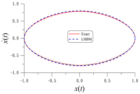
Figure 1. For a non-smooth differential equation, we compare the exact solution and the periodic solution obtained by LHBM.

Table 5. ME and $\omega$ obtained by LHBM for the harmonic analytic solutions of Equation (83) with different $q_0$. NI is the number of iterations.

$q_0$	0.95	0.98	1	1.02	1.05
ME	$4.24\times {10}^{-2}$	$6.50\times {10}^{-3}$	$2.41\times {10}^{-2}$	$4.89\times {10}^{-2}$	$8.69\times {10}^{-2}$
$\omega$	0.7317479	0.7374553	0.7412362	0.7449980	0.7506058
NI	7	7	7	7	7

4. Duffing Oscillator

In this section, we will develop a more accurate analytic solution for the Duffing oscillator by using the linearized harmonic balance method (LHBM). Consider [33]:

$$\ddot{x}\left(t\right)+x\left(t\right)+{\epsilon }_0{x}^3\left(t\right)=0,x\left(0\right)=1,\dot{x}\left(0\right)=0.$$

(88)

The Duffing equation describes the motion of a mass attached to a stretched wire, whose restoring force consists of a linear spring and a nonlinear spring. Many applications of the Duffing oscillator equation in physics can be seen in [46].

We solve

$$x^{″}\left(\theta \right)+(\delta +ϵcos2\theta )x\left(\theta \right)=e_0ϵ(3cos\theta +cos3\theta ),$$

(89)

where

$$\delta :={\displaystyle \frac{2+q_0{\epsilon }_0}{2{\omega }^2}},ϵ:={\displaystyle \frac{q_0{\epsilon }_0}{2{\omega }^2}},e_0:={\displaystyle \frac{q_0-1}{2q_0}}.$$

(90)

As shown in Figure 2, the solution obtained from Equation (89) is very accurate, with ME smaller than ${10}^{-4}$.

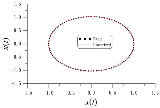
Figure 2. For the Duffing equation, we compare the exact solution and the solution obtained from the linearized equation.

We write the asymptotic solution obtained by the Lindstedt–Poincaré method (LPM) given in [33]:

$$x\left(\theta \right)=cos\theta +{\displaystyle \frac{{\epsilon }_0}{32}}(cos3\theta -cos\theta )+{\displaystyle \frac{{\epsilon }_0^2}{1024}}[23cos\theta -24cos3\theta +cos5\theta ],$$

(91)

where

$$\theta =\omega t=\left[1+{\displaystyle \frac{3{\epsilon }_0}{8}}-{\displaystyle \frac{21{\epsilon }_0^2}{256}}\right]t.$$

(92)

To proceed to the higher-order analytic solution by using the LHBM, we seek the analytic solution of Equation (89) by

$$x\left(\theta \right)=\sum _{k=1}^m{a}_{2k-1}cos(2k-1)\theta ,$$

(93)

where $a_{2k-1}$ are unknown coefficients to be determined, satisfying ${\sum }_{k=1}^m{a}_{2k-1}=1$ due to $x\left(0\right)=1$. Inserting Equation (93) into Equation (89) and taking the balance of harmonic terms, we can derive

$$\begin{array}{ccc}\hfill & & {\displaystyle \frac{ϵ}{2}}(a_1+a_3)+(\delta -1)a_1=3e_0ϵ,\hfill \end{array}$$

(94)

$$\begin{array}{ccc}\hfill & & {\displaystyle \frac{ϵ}{2}}(a_1+a_5)+(\delta -9)a_3=e_0ϵ,\hfill \end{array}$$

(95)

$$\begin{array}{ccc}\hfill & & a_{2k-3}={\displaystyle \frac{2}{ϵ}}[{(2k-1)}^2-\delta ]a_{2k-1}-a_{2k+1},k=3,\dots ,m-1,\hfill \end{array}$$

(96)

$$\begin{array}{ccc}\hfill & & a_{2m-3}={\displaystyle \frac{2}{ϵ}}[{(2m-1)}^2-\delta ]a_{2m-1},\hfill \end{array}$$

(97)

$$\begin{array}{ccc}\hfill & & \sum _{k=1}^m{a}_{2k-1}=1.\hfill \end{array}$$

(98)

When $m\ge 4$, Equation (96) is needed. When $e_0=0$, Equation (95) can be merged into Equation (96).

We take $m=3$; by means of Equations (95), (97) and (98), we have

$$\left[\begin{array}{ccc}{\displaystyle \frac{ϵ}{2}}& \delta -9& {\displaystyle \frac{ϵ}{2}}\\ 0& ϵ& 2\delta -50\\ 1& 1& 1\end{array}\right]\left[\begin{array}{c}{a}_1\\ a_3\\ a_5\end{array}\right]=\left[\begin{array}{c}{e}_0ϵ\\ 0\\ 1\end{array}\right].$$

(99)

It is easy to generate $a_1,a_3,a_5$ for each value of $\omega$, given by

$$\begin{array}{ccc}\hfill & & a_3={\displaystyle \frac{(1-2e_0)ϵ}{18-2\delta +ϵ}},\hfill \end{array}$$

(100)

$$\begin{array}{ccc}\hfill & & a_5={\displaystyle \frac{a_3ϵ}{50-2\delta }},\hfill \end{array}$$

(101)

$$\begin{array}{ccc}\hfill & & a_1=1-a_3-a_5.\hfill \end{array}$$

(102)

For $m=3$, the iteration process is given as follows.

(i)

Given ${\epsilon }_0$, $q_0$, $\epsilon$, and ${\omega }_0=1$,

(ii)

Do $j=0,1,\dots$, computing

$$\begin{array}{ccc}& & {\delta }_j={\displaystyle \frac{2+q_0{\epsilon }_0}{2{\omega }_j^2}},\hfill \\ & & {ϵ}_j={\displaystyle \frac{q_0{\epsilon }_0}{2{\omega }_j^2}},\hfill \\ & & a_{3,j}={\displaystyle \frac{(1-2e_0){ϵ}_j}{18-2{\delta }_j+{ϵ}_j}},\hfill \\ & & a_{5,j}={\displaystyle \frac{a_{3,j}{ϵ}_j}{50-2{\delta }_j}},\hfill \\ & & a_{1,j}=1-a_{3,j}-a_{5,j},\hfill \end{array}$$

(iii)

Computing

$${\omega }_{j+1}=\sqrt{1+{\displaystyle \frac{3q_0{\epsilon }_0}{4}}+{\displaystyle \frac{q_0{\epsilon }_0(a_{3,j}-6e_0)}{4a_{1,j}}}}$$

(103)

derived from Equation (94) by inserting Equation (90) for $\delta$ and $ϵ$,

(iv)

If $|{\omega }_{j+1}-{\omega }_j|<\epsilon$ then stop; otherwise, go to (ii). Obviously, we cannot take ${\omega }_0=0$, which would render the iteration a failure.

We take $q_0$ to be the optimal value. In Table 6 for different ${\epsilon }_0$, we compare ME1 obtained by LHBM within one period to the exact solution, and at the same time, we compare $\omega$ obtained from Equations (92) and (103); the exact $\omega$ is given by

$$\omega =\pi {\left(2\sqrt{2}{\int }_0^{\pi /2}{\displaystyle \frac{d\theta }{\sqrt{2+{\epsilon }_0(1+{sin}^2\theta )}}}\right)}^{-1}.$$

(104)

Table 6. ME1 and ME2 for two type harmonic solutions of Equation (88) with different ${\epsilon }_0$ and comparing $\omega$ obtained from Equations (92), (103), (115) and (104). NI is the number of iterations.

${\epsilon }_0$	0.1	0.2	0.4	0.8	1.0	1.5
$q_0$	2.987	2.975	2.958	2.93	2.92	2.899
NI	5	6	7	8	9	10
ME1	$2.03\times {10}^{-7}$	$1.21\times {10}^{-6}$	$1.16\times {10}^{-5}$	$3.72\times {10}^{-5}$	$5.83\times {10}^{-5}$	$7.84\times {10}^{-5}$
ME2	$1.71\times {10}^{-4}$	$1.24\times {10}^{-3}$	$8.36\times {10}^{-3}$	$1.51\times {10}^{-2}$	$5.08\times {10}^{-2}$	$8.86\times {10}^{-2}$
Equation (92)	1.03668	1.07172	1.13688	1.24750	1.29297	1.37793
Equation (103)	1.03672	1.07200	1.13891	1.26118	1.31777	1.44913
Exact $\omega$	1.03672	1.07200	1.13891	1.26118	1.31778	1.44913

Upon comparing to ME2 obtained from Equation (91), the present periodic solutions are more accurate. Upon comparing to Table 3 in [41], the accuracy of LHBM is very good, even better than that obtained by the LLPM.

Instead of $\omega$, we can also derive an iteration method in terms $\delta$ directly. It follows from Equation (90) that

$$\begin{array}{ccc}\hfill & & \delta ={\displaystyle \frac{1}{{\omega }^2}}+ϵ,ϵ={\displaystyle \frac{q_0{\epsilon }_0\delta }{2+q_0{\epsilon }_0}},\hfill \end{array}$$

(105)

$$\begin{array}{ccc}\hfill & & {\displaystyle \frac{2}{ϵ}}={\displaystyle \frac{4+2q_0{\epsilon }_0}{q_0{\epsilon }_0\delta }}.\hfill \end{array}$$

(106)

Inserting it for $2/ϵ$ into Equations (95)–(97) generates an iteration method in terms of $\delta$:

$$\begin{array}{ccc}\hfill & & a_1={\displaystyle \frac{4+2q_0{\epsilon }_0}{q_0{\epsilon }_0\delta }}(9-\delta )a_3-a_5+2e_0,\hfill \end{array}$$

(107)

$$\begin{array}{ccc}\hfill & & a_{2k-3}={\displaystyle \frac{4+2q_0{\epsilon }_0}{q_0{\epsilon }_0\delta }}[{(2k-1)}^2-\delta ]a_{2k-1}-a_{2k+1},k=3,\dots ,m-1,\hfill \end{array}$$

(108)

$$\begin{array}{ccc}\hfill & & a_{2m-3}={\displaystyle \frac{4+2q_0{\epsilon }_0}{q_0{\epsilon }_0\delta }}[{(2m-1)}^2-\delta ]a_{2m-1}.\hfill \end{array}$$

(109)

By means of Equations (98) and (107)–(109), it is easy to compute $a_1,a_3,a_5$ for each value of $\delta$ given by

$$\begin{array}{ccc}\hfill & & a_3={\displaystyle \frac{q_0{\epsilon }_0\delta (1-2e_0)}{9(4+2q_0{\epsilon }_0)-(4+q_0{\epsilon }_0)\delta }},\hfill \end{array}$$

(110)

$$\begin{array}{ccc}\hfill & & a_5={\displaystyle \frac{q_0{\epsilon }_0\delta a_3}{(4+2q_0{\epsilon }_0)(25-\delta )}},\hfill \end{array}$$

(111)

$$\begin{array}{ccc}\hfill & & a_1=1-a_3-a_5.\hfill \end{array}$$

(112)

Inserting Equation (106) into Equation (94) yields

$${\delta }_{j+1}={\displaystyle \frac{(4+2q_0{\epsilon }_0)a_{1,j}}{(4+3q_0{\epsilon }_0)a_{1,j}+q_0{\epsilon }_0{a}_{3,j}-6e_0{q}_0{\epsilon }_0}},j=0,1,\dots ,$$

(113)

where $a_{1,j}$ and $a_{3,j}$ are calculated from Equations (110)–(112) by inserting ${\delta }_j$. The initial guess of ${\delta }_0$ can be any ${\delta }_0>0$, say ${\delta }_0=0.5$.

It follows from Equation (105) that

$${\displaystyle \frac{1}{{\omega }^2}}=\delta -ϵ={\displaystyle \frac{2\delta }{2+q_0{\epsilon }_0}},$$

(114)

and thus, a simple formula for $\omega$ is available as follows:

$$\omega =\sqrt{{\displaystyle \frac{2+q_0{\epsilon }_0}{2\delta }}}.$$

(115)

When the convergent value $\delta$ is obtained, inserting it into the above equation, we can compute $\omega$. We found that this iteration converges very fast with a few steps.

We take $m=3$ and $q_0$ to be the optimal value. In Table 7 for different ${\epsilon }_0$, we compare the ME obtained by the second harmonic balance method to the exact solution obtained by RK4 to integrate Equation (88), and at the same time, we list $\omega$ obtained from Equations (104) and (115). Comparing to Table 6, the presented two type harmonic solutions are almost the same. Upon comparing to Table 3 in [41], the accuracy of LHBM is very good, even better than that obtained by the LLPM.

Table 7. ME for second harmonic solutions of Equation (88) with different ${\epsilon }_0$ and comparing $\omega$ obtained from Equations (104) and (115). NI is the number of iterations.

${\epsilon }_0$	0.1	0.2	0.4	0.8	1.0	1.5
$q_0$	2.987	2.975	2.958	2.93	2.92	2.899
NI	6	6	7	8	9	10
ME	$2.03\times {10}^{-7}$	$1.51\times {10}^{-6}$	$1.16\times {10}^{-5}$	$3.72\times {10}^{-5}$	$5.83\times {10}^{-5}$	$7.84\times {10}^{-5}$
ME of Equation (123)	$4.92\times {10}^{-3}$	$9.93\times {10}^{-3}$	$1.97\times {10}^{-2}$	$3.72\times {10}^{-2}$	$4.47\times {10}^{-2}$	$6.03\times {10}^{-2}$
Equation (115)	1.03672	1.07200	1.13891	1.26118	1.31777	1.44913
Exact $\omega$	1.03672	1.07200	1.13891	1.26118	1.31778	1.44913
Equation (124)	1.03441	1.06771	1.13137	1.24899	1.30384	1.43178

By using

$$x\left(t\right)=By\left(t\right),$$

(116)

we can transform Equations (28) and (29) to

$$\begin{array}{ccc}\hfill & & \ddot{y}\left(t\right)+B^2{y}^3\left(t\right)=0,\hfill \end{array}$$

(117)

$$\begin{array}{ccc}\hfill & & y\left(0\right)=1,\dot{y}\left(0\right)=0.\hfill \end{array}$$

(118)

They are a special case of Equation (88) with ${\epsilon }_0=B^2$ by deleting $x\left(t\right)$.

We can apply the LHBM to find the third-order periodic solution of Equations (28) and (29) by

$$\begin{array}{ccc}\hfill & & a_3={\displaystyle \frac{(1-2e_0)ϵ}{18-ϵ}},\hfill \end{array}$$

(119)

$$\begin{array}{ccc}\hfill & & a_5={\displaystyle \frac{a_3ϵ}{50-2ϵ}},\hfill \end{array}$$

(120)

$$\begin{array}{ccc}\hfill & & a_1=1-a_3-a_5,\hfill \end{array}$$

(121)

$$\begin{array}{ccc}\hfill & & {\omega }_{j+1}=\sqrt{{\displaystyle \frac{3q_0{\epsilon }_0}{4}}+{\displaystyle \frac{q_0{\epsilon }_0(a_3-6e_0)}{4a_1}}},j=0,1,\dots .\hfill \end{array}$$

(122)

We take $B=1$. Upon comparing to ME2 = $1.996\times {10}^{-2}$ obtained from Equation (36), the present harmonic solution with the error denoted by ME1 = $7.518\times {10}^{-4}$ is more accurate. The improvement of accuracy is about two orders. By using the original HBM, it is hard to find the analytic periodic solutions with order greater than three, because the procedure is very complicated. In contrast, the LHBM can be easily used to find the higher-order analytic periodic solutions of nonlinear oscillators.

According to the result in [33] the periodic solution of Equation (88) is

$$x\left(t\right)=cos\left(\sqrt{1+{\displaystyle \frac{3{\epsilon }_0}{4}}}t\right).$$

(123)

The error obtained by this equation is denoted as ME of Equation (123). As tabulated in Table 7, the present harmonic solution with the error denoted by ME is more accurate. The improvement of accuracy is about three to four orders.

According to He’s formula [18], we have

$$\omega =\sqrt{1+{\displaystyle \frac{7{\epsilon }_0{B}^2}{10}}},$$

(124)

where $B=1$ for Equation (88). In Table 7 we can observe that the accuracy of the frequency obtained by the Hamiltonian-based frequency–amplitude formulation is of the order ${10}^{-2}$. However, owing to its simplicity, it can be applied to a more complex conservative system.

We extend Equation (88) to

$$\ddot{x}\left(t\right)+x\left(t\right)+{\epsilon }_0{x}^3\left(t\right)=0,x\left(0\right)=B,\dot{x}\left(0\right)=0.$$

(125)

We can derive the same Equation (89), but with

$$\delta :={\displaystyle \frac{2+q_0{\epsilon }_0{B}^2}{2{\omega }^2}},ϵ:={\displaystyle \frac{q_0{\epsilon }_0{B}^2}{2{\omega }^2}},e_0:={\displaystyle \frac{(q_0-1)B}{2q_0}}.$$

(126)

By using the HBM, it is hard to derive the frequency–amplitude formula; however, if we take $m=2$ and use the following equations derived from the LHBM:

$$\begin{array}{ccc}\hfill & & a_1+a_3=B,\hfill \end{array}$$

(127)

$$\begin{array}{ccc}\hfill & & {\displaystyle \frac{ϵ}{2}}(a_1+a_3)+(\delta -1)a_1=3e_0ϵ,\hfill \end{array}$$

(128)

$$\begin{array}{ccc}\hfill & & {\displaystyle \frac{ϵ}{2}}{a}_1+(\delta -9)a_3=e_0ϵ,\hfill \end{array}$$

(129)

we can derive the following formula to determine the frequency:

$$\begin{array}{ccc}\hfill & & \omega =\sqrt{{\displaystyle \frac{1}{72}}\left[b_0+\sqrt{b_0^2-36a_0}\right]},\hfill \end{array}$$

(130)

$$\begin{array}{ccc}\hfill & & a_0=5q_0{\epsilon }_0^2{B}^4+4(q_0+4){\epsilon }_0{B}^2+16,b_0=(q_0+28){\epsilon }_0{B}^2+40.\hfill \end{array}$$

(131)

In Table 8, the exact value of $\omega$ is compared to that computed by Equations (124) and (130). The improvement of the frequency obtained by Equation (130) compared to that obtained by Equation (124) is about five orders.

Table 8. Comparing frequency with different values of ${\epsilon }_0{B}^2$ for Equation (125).

${\epsilon }_0{B}^2$	0.1	1	2	3	5	10
$q_0$	2.996	2.969	2.954	2.9456	2.936	2.9264
Exact $\omega$	1.0367169	1.3177761	1.5691058	1.7844191	2.1504162	2.8666401
Equation (130)	1.0367169	1.3177763	1.5691079	1.7844195	2.1504174	2.8666397
Equation (124)	1.0344081	1.3038405	1.5491933	1.7606817	2.1213203	2.8284271

Applying the LHBM to Equation (125) with $m=2$, we can derive the following periodic solution:

$$x\left(t\right)={\displaystyle \frac{(2q_0-3){\epsilon }_0{B}^3}{4-4{\omega }^2+2q_0{\epsilon }_0{B}^2}}cos\left(\omega t\right)+\left[B-{\displaystyle \frac{(2q_0-3){\epsilon }_0{B}^3}{4-4{\omega }^2+2q_0{\epsilon }_0{B}^2}}\right]cos\left(3\omega t\right),$$

(132)

where $\omega$ is given by Equation (130).

By using the dual Lagrange multiplier approach for Equation (125), Anjum and He [17] can derive the following periodic solution:

$$x\left(t\right)=Bcos\left(\omega t\right)-{\displaystyle \frac{{\epsilon }_0{B}^3}{32{\omega }^2}}cos\left(\omega t\right)+{\displaystyle \frac{{\epsilon }_0{B}^3}{32{\omega }^2}}cos\left(3\omega t\right),$$

(133)

where

$$\omega =\sqrt{1+{\displaystyle \frac{3{\epsilon }_0{B}^2}{4}}}.$$

(134)

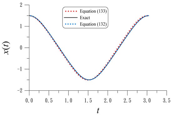
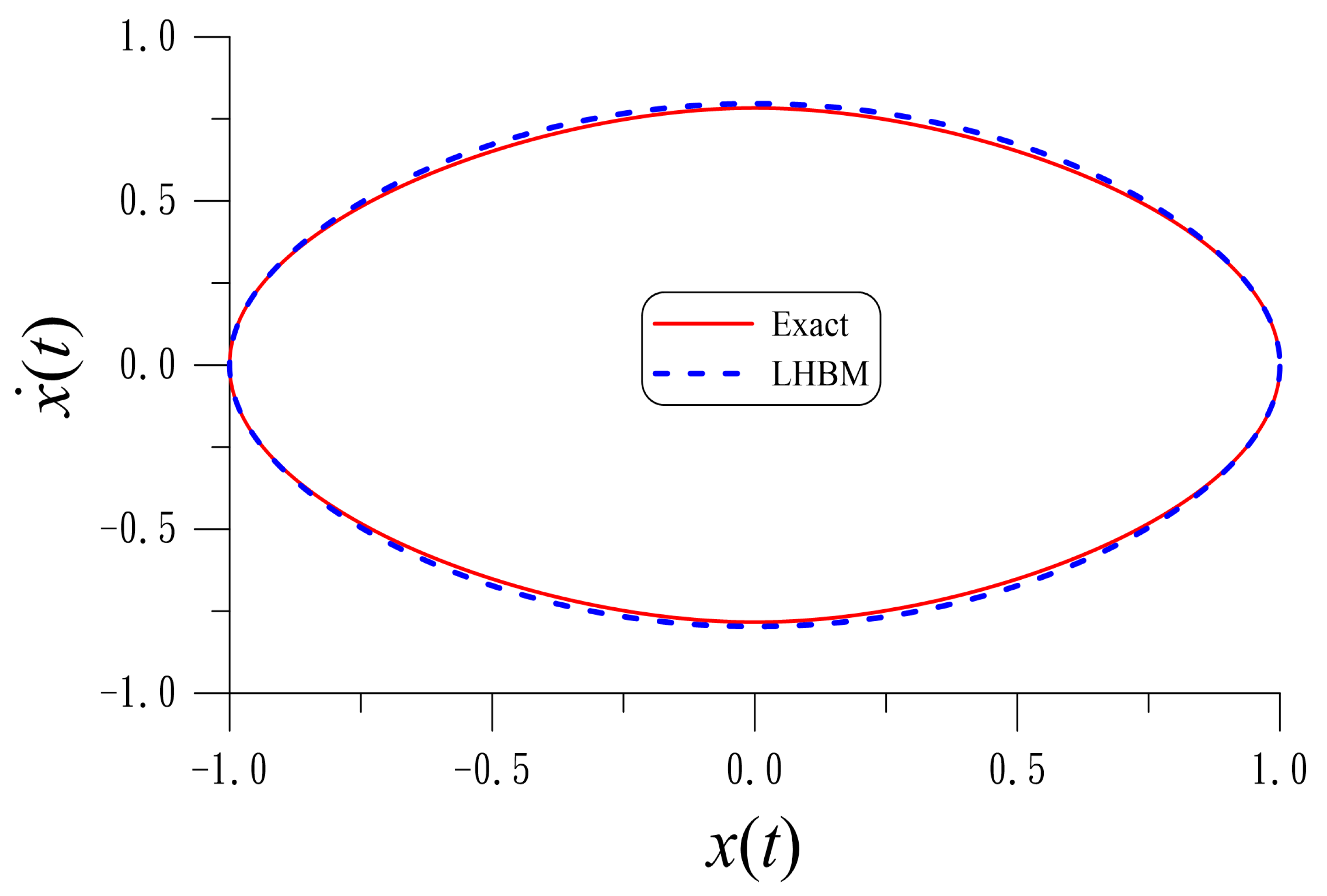
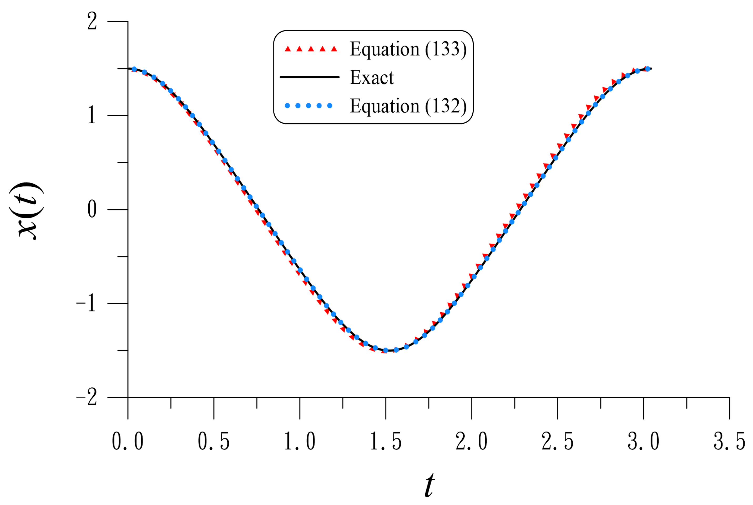
In Table 9, for different values of B and a fixed ${\epsilon }_0=2$, we compare the ME obtained by Equations (132) and (133). The accuracy of LHBM is very good, better than that obtained by the dual Lagrange multiplier approach by about one or two orders.

Table 9. MEs for Equations (132) and (133) with different values of B.

B	0.1	0.4	0.8	1.0	1.5
$q_0$	2.999	2.987	2.964	2.954	2.938
ME of Equation (132)	$6.88\times {10}^{-8}$	$4.60\times {10}^{-5}$	$5.71\times {10}^{-4}$	$1.06\times {10}^{-3}$	$2.61\times {10}^{-3}$
ME of Equation (133)	$2.16\times {10}^{-6}$	$1.45\times {10}^{-3}$	$1.82\times {10}^{-2}$	$3.41\times {10}^{-2}$	$8.54\times {10}^{-2}$

Figure 3 compares the exact solution and the periodic solutions obtained by Equations (132) and (133) for the Duffing oscillator with ${\epsilon }_{0}B=4.5$. It can be seen that the periodic solution obtained from Equation (132) is almost coincident with the exact solution. It is apparent that the periodic solution obtained from Equation (132) is more accurate than that obtained from Equation (133).

Figure 3. For the Duffing oscillator in Equation (125), we compare the exact solution and the periodic solutions obtained by Equations (132) and (133).

5. Third-Order Nonlinear Jerk Oscillators

5.1. First-Type Nonlinear Jerk Oscillator

We demonstrate the linearized harmonic balance method (LHBM) for analytically finding a periodic solution of a nonlinear jerk equation:

$$\stackrel{⃛}{x}+\dot{x}=x\dot{x}\ddot{x},$$

(135)

where

$$x\left(0\right)=0,\dot{x}\left(0\right)={\epsilon }_0,\ddot{x}\left(0\right)=0.$$

(136)

We linearize Equation (135) around

$$x_0\left(t\right)={\displaystyle \frac{{\epsilon }_0}{\omega }}sin\omega t,$$

(137)

to obtain

$$\stackrel{⃛}{x}+\dot{x}-q_0{x}_0{\ddot{x}}_0\dot{x}=(1-q_0)x_0{\dot{x}}_0{\ddot{x}}_0,$$

(138)

where $q_0$ is a weight factor. Inserting

$$x_0{\ddot{x}}_0=-{\epsilon }_0^2{sin}^2\omega t={\displaystyle \frac{{\epsilon }_0^2}{2}}(cos2\omega t-1),x_0{\dot{x}}_0{\ddot{x}}_0=-{\epsilon }_0^{3}cos\omega t{sin}^2\omega t={\displaystyle \frac{{\epsilon }_0^3}{4}}(cos3\omega t-cos\omega t)$$

into Equation (138) renders

$$\stackrel{⃛}{x}+\left[1+{\displaystyle \frac{q_0{\epsilon }_0^2}{2}}-{\displaystyle \frac{q_0{\epsilon }_0^2}{2}}cos2\omega t\right]\dot{x}=e_{0}cos3\omega t-e_{0}cos\omega t,$$

(139)

where

$$e_0:={\displaystyle \frac{(1-q_0){\epsilon }_0^3}{4}}.$$

(140)

In terms of $\theta =\omega t$, Equation (139) is recast to

$$x^{‴}\left(\theta \right)+(\delta +ϵcos2\theta )x^{\prime }\left(\theta \right)={\displaystyle \frac{e_0}{{\omega }^3}}(cos3\theta -cos\theta ),$$

(141)

where

$$\delta :={\displaystyle \frac{2+q_0{\epsilon }_0^2}{2{\omega }^2}},ϵ:=-{\displaystyle \frac{q_0{\epsilon }_0^2}{2{\omega }^2}}.$$

(142)

We seek the periodic solution for Equation (141) by the following Fourier series:

$$\begin{array}{ccc}\hfill & & x\left(\theta \right)=\sum _{k=1}^m{b}_{2k-1}sin(2k-1)\theta ,\hfill \end{array}$$

(143)

$$\begin{array}{ccc}\hfill & & y\left(\theta \right)=x^{\prime }\left(\theta \right)=\sum _{k=1}^m{a}_{2k-1}cos(2k-1)\theta ,\hfill \end{array}$$

(144)

where $a_{2k-1}=(2k-1)b_{2k-1}$ satisfies the constraint:

$$\sum _{k=1}^m{a}_{2k-1}={\displaystyle \frac{{\epsilon }_0}{\omega }},$$

(145)

owing to $x^{\prime }\left(0\right)={\epsilon }_0/\omega$.

Setting $y\left(\theta \right)=x^{\prime }\left(\theta \right)$ in Equation (141), we come to a nonhomogeneous Mathieu-type ODE for $y\left(\theta \right)$:

$$y^{″}\left(\theta \right)+(\delta +ϵcos2\theta )y\left(\theta \right)={\displaystyle \frac{e_0}{{\omega }^3}}(cos3\theta -cos\theta ),$$

(146)

which has the same form as Equation (89).

By the same token, we can derive

$$\begin{array}{ccc}\hfill & & {\displaystyle \frac{ϵ}{2}}(a_1+a_3)+(\delta -1)a_1=-{\displaystyle \frac{e_0}{{\omega }^3}},\hfill \end{array}$$

(147)

$$\begin{array}{ccc}\hfill & & {\displaystyle \frac{ϵ}{2}}(a_1+a_5)+(\delta -9)a_3={\displaystyle \frac{e_0}{{\omega }^3}},\hfill \end{array}$$

(148)

$$\begin{array}{ccc}\hfill & & a_{2k-3}={\displaystyle \frac{2}{ϵ}}[{(2k-1)}^2-\delta ]a_{2k-1}-a_{2k+1},k=3,\dots ,m-1,\hfill \end{array}$$

(149)

$$\begin{array}{ccc}\hfill & & a_{2m-3}={\displaystyle \frac{2}{ϵ}}[{(2m-1)}^2-\delta ]a_{2m-1}.\hfill \end{array}$$

(150)

We can derive an iteration method in terms of $\delta$ directly. From Equation (142), we have

$$\delta ={\displaystyle \frac{1}{{\omega }^2}}-ϵ,ϵ=-{\displaystyle \frac{q_0{\epsilon }_0^2\delta }{2+q_0{\epsilon }_0^2}}.$$

(151)

Upon inserting Equation (142) into Equations (148) and (150) and using Equation (145), we generate an iteration method in terms of $\delta$:

$$\begin{array}{ccc}\hfill & & a_3={\displaystyle \frac{4e_0+q_0{\epsilon }_0^3}{(4+3q_0{\epsilon }_0^2)\omega -36{\omega }^3}},\hfill \end{array}$$

(152)

$$\begin{array}{ccc}\hfill & & a_5={\displaystyle \frac{q_0{\epsilon }_0^2{a}_3}{4+2q_0{\epsilon }_0^2-100{\omega }^2}},\hfill \end{array}$$

(153)

$$\begin{array}{ccc}\hfill & & a_1={\displaystyle \frac{{\epsilon }_0}{\omega }}-a_3-a_5,\hfill \end{array}$$

(154)

where

$$\omega =\sqrt{{\displaystyle \frac{2+q_0{\epsilon }_0^2}{2\delta }}}$$

(155)

is deduced from Equation (151) by writing it as

$${\displaystyle \frac{1}{{\omega }^2}}=\delta +ϵ={\displaystyle \frac{2\delta }{2+q_0{\epsilon }_0^2}}.$$

(156)

To describe the iteration technique, the iteration process is summarized as follows for $m=3$.

(i)

Given ${\epsilon }_0$, $q_0$, $\epsilon$, and ${\delta }_0$,

(ii)

Do $j=0,1,\dots$, computing

$$\begin{array}{ccc}& & {\omega }_j=\sqrt{{\displaystyle \frac{2+q_0{\epsilon }_0^2}{2{\delta }_j}}},\hfill \\ & & a_{3,j}={\displaystyle \frac{4e_0+q_0{\epsilon }_0^3}{(4+3q_0{\epsilon }_0^2){\omega }_j-36{\omega }_j^3}},\hfill \\ & & a_{5,j}={\displaystyle \frac{q_0{\epsilon }_0^2{a}_{3,j}}{4+2q_0{\epsilon }_0^2-100{\omega }_j^2}},\hfill \\ & & a_{1,j}={\displaystyle \frac{{\epsilon }_0}{{\omega }_j}}-a_{3,j}-a_{5,j},\hfill \end{array}$$

(iii)

Computing

$${\delta }_{j+1}={\displaystyle \frac{(4+2q_0{\epsilon }_0^2)(a_{1,j}-e_0/{\omega }_j^3)}{(4+q_0{\epsilon }_0^2)a_{1,j}-q_0{\epsilon }_0^2{a}_{3,j}}}$$

(157)

derived by inserting Equation (151) into Equation (147),

(iv)

If $|{\delta }_{j+1}-{\delta }_j|<\epsilon$ then stop; otherwise, go to (ii).

The initial guess of ${\delta }_0$ can be any ${\delta }_0>0$, say ${\delta }_0=0.5$. When the convergent value $\delta$ is obtained, inserting it into the above equation, we can compute $\omega$. We found that this iteration converges very fast with a few steps, subjecting to $|{\delta }_{j+1}-{\delta }_j|<{10}^{-10}$.

We take $m=3$ and fix ${\epsilon }_0=0.5$. The convergence behavior is not sensitive to the initial guess of ${\delta }_0$, and we list the number of iterations (NI) for different values of ${\delta }_0$. For ${\delta }_0=0.1$, we have NI = 9; for ${\delta }_0=0.5$, we have NI = 9; for ${\delta }_0=1$, we have NI = 8; for ${\delta }_0=1.5$, we have NI = 9; and for ${\delta }_0=2$, we have NI = 9.

The periodic solution of Equation (135) up to the second order was derived in [32] by using He’s homotopy perturbation method:

$$x\left(t\right)={\displaystyle \frac{{\epsilon }_0}{{\omega }_1}}sin{\omega }_{1}t+D(sin{\omega }_{1}t+sin3{\omega }_{1}t)+E\left(23sin{\omega }_{2}t-12sin3{\omega }_{2}t+{\displaystyle \frac{13}{15}}sin5{\omega }_{2}t\right),$$

(158)

where

$$\begin{array}{ccc}\hfill & & {\alpha }_1={\displaystyle \frac{{\epsilon }_0^2}{4}},{\alpha }_2=-{\displaystyle \frac{{\epsilon }_{0}D{\omega }_1}{12}},D=-{\displaystyle \frac{{\epsilon }_0^3}{32{\omega }_1^3}},E={\displaystyle \frac{{\epsilon }_0^{2}D}{288{\omega }_2^2}},\hfill \end{array}$$

(159)

$$\begin{array}{ccc}\hfill & & {\omega }_1=\sqrt{1+{\alpha }_1},{\omega }_2=\sqrt{1+{\alpha }_1+{\alpha }_2}.\hfill \end{array}$$

(160)

We take $m=3$, and the optimal value of $q_0$ is obtained by minimizing the value of ME. Table 10 compares the results with different ${\epsilon }_0$, where ME1 is for Equation (143). Apparently, the present ME1 is very small, better than ME2 for Equation (158) obtained by Ma et al. [32].

Table 10. The LHBM is applied to Equations (135) and (136) with different values of ${\epsilon }_0$; NI signifies the number of iterations spent in LHBM. The maximal errors of Equations (143) and (158) are denoted as ME1 and ME2, respectively. The period $T=2\pi /\omega$ obtained by LHBM, obtained in [32], and the exact one are compared.

${\epsilon }_0$	0.1	0.2	0.5	1	2
$q_0$	0.26	0.33	0.25	0.21	0.21
NI	5	6	9	14	42
ME1	$4.00\times {10}^{-8}$	$1.31\times {10}^{-6}$	$1.12\times {10}^{-4}$	$2.58\times {10}^{-3}$	$3.70\times {10}^{-2}$
ME2	$8.16\times {10}^{-8}$	$2.59\times {10}^{-6}$	$2.38\times {10}^{-4}$	$6.16\times {10}^{-3}$	$9.67\times {10}^{-2}$
Exact T	6.275347	6.252016	6.096061	5.626007	4.491214
Ma et al. [32]	6.275347	6.252016	6.096025	5.624541	4.466205
Equation (155)	6.275347	6.252016	6.096238	5.627753	4.480898

For the periodic vibration problem, the period T is the major quantity to be determined. As shown in Table 10, the period T obtained by the LHBM is more accurate than that obtained by Ma et al. [32], when ${\epsilon }_0$ is greater than 1. Also, the accuracy of the periodic solution is improved twice. For a larger value of ${\epsilon }_0$, the improvement is of about one order.

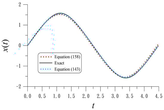
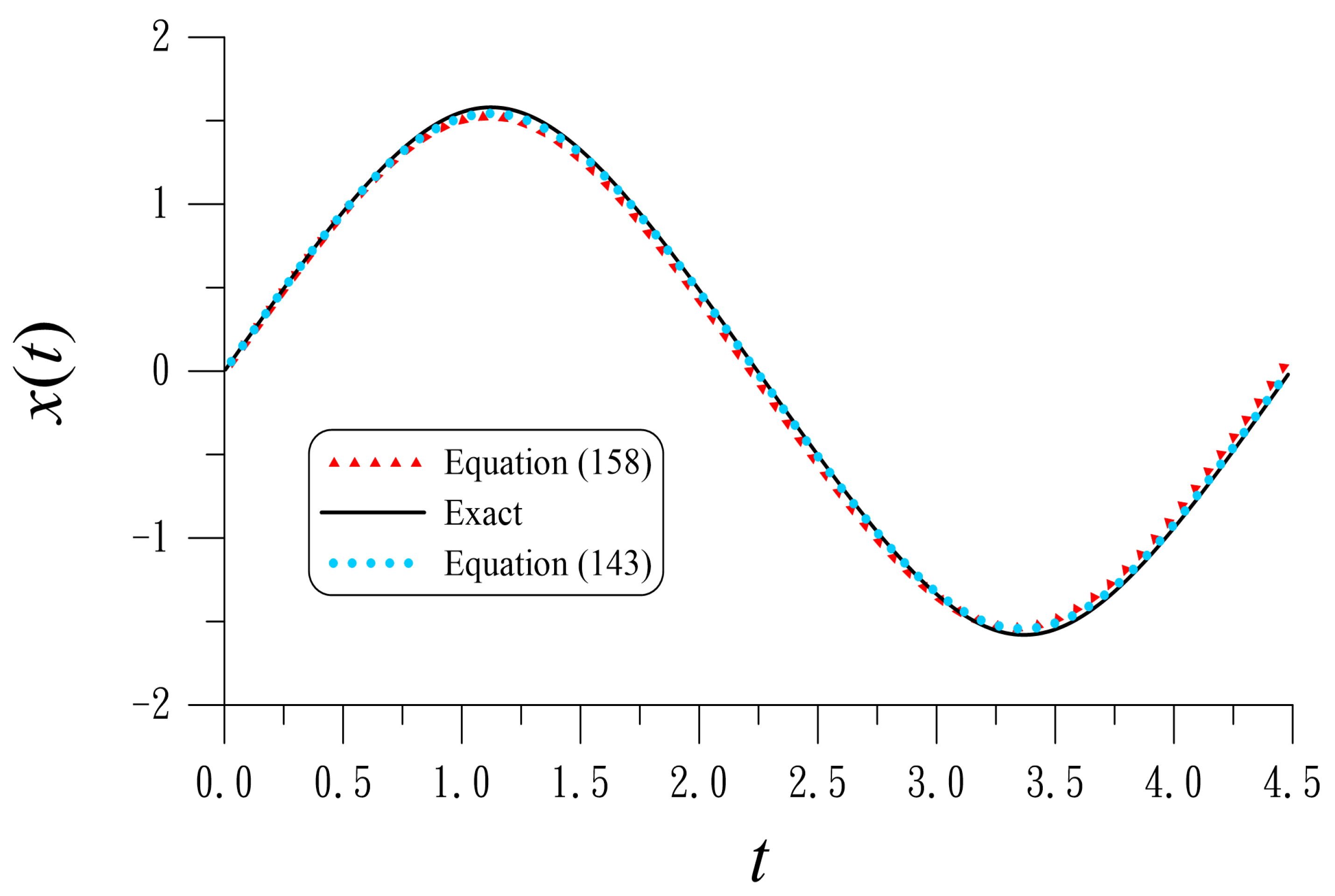
Figure 4 compares the exact solution and the periodic solutions obtained by Equations (143) and (158) for the jerk oscillator with ${\epsilon }_0=2$. It can be seen that the periodic solution obtained from Equation (143) is almost coincident with the exact solution. It is apparent that the periodic solution obtained from Equation (143) is more accurate than that obtained from Equation (158).

Figure 4. For the nonlinear jerk oscillator in Equation (135), we compare the exact solution and the periodic solutions obtained by Equations (143) and (158).

5.2. Second-Type Nonlinear Jerk Oscillator

We consider

$$\stackrel{⃛}{x}+\dot{x}+\dot{x}{\ddot{x}}^2=0,$$

(161)

where

$$x\left(0\right)=0,\dot{x}\left(0\right)={\epsilon }_0,\ddot{x}\left(0\right)=0.$$

(162)

Using Equation (137) and linearizing Equation (161) around $x_0\left(t\right)$ generates

$$\stackrel{⃛}{x}+\left[1+{\displaystyle \frac{q_0{\epsilon }_0^2{\omega }^2}{2}}-{\displaystyle \frac{q_0{\epsilon }_0^2{\omega }^2}{2}}cos2\omega t\right]\dot{x}=e_0{\omega }^2[cos3\omega t-cos\omega t],$$

(163)

where $e_0$ is still defined by Equation (140).

In terms of $\theta =\omega t$, Equation (163) is recast to

$$x^{‴}\left(\theta \right)+(\delta +ϵcos2\theta )x^{\prime }\left(\theta \right)={\displaystyle \frac{e_0}{\omega }}(cos3\theta -cos\theta ),$$

(164)

where $\delta$ and $ϵ$ are still defined by Equation (142).

Similarly, we can derive

$$\begin{array}{ccc}\hfill & & {\displaystyle \frac{ϵ}{2}}(a_1+a_3)+(\delta -1)a_1=-{\displaystyle \frac{e_0}{\omega }},\hfill \end{array}$$

(165)

$$\begin{array}{ccc}\hfill & & {\displaystyle \frac{ϵ}{2}}(a_1+a_5)+(\delta -9)a_3={\displaystyle \frac{e_0}{\omega }},\hfill \end{array}$$

(166)

$$\begin{array}{ccc}\hfill & & a_{2k-3}={\displaystyle \frac{2}{ϵ}}[{(2k-1)}^2-\delta ]a_{2k-1}-a_{2k+1},k=3,\dots ,m-1,\hfill \end{array}$$

(167)

$$\begin{array}{ccc}\hfill & & a_{2m-3}={\displaystyle \frac{2}{ϵ}}[{(2m-1)}^2-\delta ]a_{2m-1}.\hfill \end{array}$$

(168)

We take $m=3$ to obtain three linear equations:

$$\begin{array}{ccc}\hfill & & {\displaystyle \frac{ϵ}{2}}(a_1+a_5)+(\delta -9)a_3={\displaystyle \frac{e_0}{\omega }},\hfill \end{array}$$

(169)

$$\begin{array}{ccc}\hfill & & a_3={\displaystyle \frac{2}{ϵ}}[25-\delta ]a_5,\hfill \end{array}$$

(170)

$$\begin{array}{ccc}\hfill & & a_1+a_3+a_5={\displaystyle \frac{{\epsilon }_0}{\omega }}.\hfill \end{array}$$

(171)

By solving them, we can generate an iteration method in terms of $\delta$:

$$\begin{array}{ccc}\hfill & & a_3={\displaystyle \frac{4{\omega }^2{e}_0+q_0{\epsilon }_0^3}{(4+3q_0{\epsilon }_0^2)\omega -36{\omega }^3}},\hfill \end{array}$$

(172)

$$\begin{array}{ccc}\hfill & & a_5={\displaystyle \frac{q_0{\epsilon }_0^2{a}_3}{4+2q_0{\epsilon }_0^2-100{\omega }^2}},\hfill \end{array}$$

(173)

$$\begin{array}{ccc}\hfill & & a_1={\displaystyle \frac{{\epsilon }_0}{\omega }}-a_3-a_5,\hfill \end{array}$$

(174)

where

$$\omega =\sqrt{{\displaystyle \frac{2+q_0{\epsilon }_0^2}{2\delta }}}.$$

(175)

The iteration process is summarized as follows for $m=3$.

(i)

Given ${\epsilon }_0$, $q_0$, $\epsilon$, and ${\delta }_0\ne 0$,

(ii)

Do $j=0,1,\dots$, computing

$$\begin{array}{ccc}& & {\omega }_j=\sqrt{{\displaystyle \frac{2+q_0{\epsilon }_0^2}{2{\delta }_j}}},\hfill \\ & & a_{3,j}={\displaystyle \frac{4{\omega }_j^2{e}_0+q_0{\epsilon }_0^3}{(4+3q_0{\epsilon }_0^2){\omega }_j-36{\omega }_j^3}},\hfill \\ & & a_{5,j}={\displaystyle \frac{q_0{\epsilon }_0^2{a}_{3,j}}{4+2q_0{\epsilon }_0^2-100{\omega }_j^2}},\hfill \\ & & a_{1,j}={\displaystyle \frac{{\epsilon }_0}{{\omega }_j}}-a_{3,j}-a_{5,j},\hfill \end{array}$$

(iii)

Computing

$${\delta }_{j+1}={\displaystyle \frac{(4+2q_0{\epsilon }_0^2)(a_{1,j}-e_0/{\omega }_j)}{(4+q_0{\epsilon }_0^2)a_{1,j}-q_0{\epsilon }_0^2{a}_{3,j}}}$$

(176)

derived by inserting Equation (151) into Equation (165),

(iv)

If $|{\delta }_{j+1}-{\delta }_j|<\epsilon$ then stop; otherwise, go to (ii). We found that this iteration converges very fast, in at most eight iterations. By the same token, we cannot take ${\delta }_0=0$ to avoid the zero denominator.

The optimal value of $q_0$ is obtained by minimizing the maximum error of periodic solution. Table 11 compares the results with different values of ${\epsilon }_0$, where ME for Equation (143) is compared with that computed by RK4 on Equations (161) and (162) within one period $T=2\pi /\omega$. Apparently, the present ME is very small. When the amplitude ${\epsilon }_0$ is increased, the period obtained by the LHBM is more accurate than that obtained in [28,32].

Table 11. The LHBM is applied to Equations (161) and (162) with different values of ${\epsilon }_0$; ME denotes the maximal errors, and NI signifies the number of iterations spent in LHBM. The period $T=2\pi /\omega$ obtained by LHBM, obtained in [28,32], and the exact one are compared.

${\epsilon }_0$	0.1	0.2	0.5	1	1.5
$q_0$	0.37	0.335	0.345	0.383	0.445
NI	4	4	5	6	8
ME	$6.56\times {10}^{-8}$	$2.21\times {10}^{-6}$	$2.10\times {10}^{-4}$	$6.01\times {10}^{-3}$	$3.66\times {10}^{-2}$
Exact T	6.275334	6.251809	6.088449	5.527200	4.690247
Rahman et al. [28]	6.275334	6.251809	6.088450	5.527497	4.683270
Ma et al. [32]	6.275334	6.251808	6.088129	5.506308	4.426855
Equation (175)	6.275334	6.251809	6.088449	5.527286	4.690303

As shown in Table 11, the period T obtained by the LHBM is more accurate than that obtained by Ma et al. [32] for all ${\epsilon }_0$. When ${\epsilon }_0$ is greater than 0.5, the period T obtained by the LHBM is more accurate than that obtained by Rahman et al. [28], who derived the periodic solution of the jerk equation by using a modified harmonic balance method. The procedure in [28] is very complicated, and is needed to solve four highly nonlinear coupled equations.

6. Conclusions

To simplify the traditional harmonic balance method (HBM), a new analytic method based on a linearization technique was executed on the nonlinear differential equations, and then we applied the HBM to solve the non-homogeneous Mathieu-type ODE with periodic forcing terms on the right-hand side. The presented linearized HBM (LHBM), with linearized recursion method and linear system, is easily carried out with merely a few linear terms appearing in the iteration process for each order approximation of the analytic solution. Compared to the original nonlinear harmonic balance method, the LHBM can save many algebraic manipulations. A linearization process was used after introducing a simple weight factor to avoid the complex nonlinear algebraic equations, which are the main disadvantage of HBM. The optimal value of weight factor was determined by minimizing the absolute error of periodic solution within one period compared to that computed by RK4. The determination of Fourier coefficients and the frequency of vibration converges very fast within, in at most ten iterations, with a stringent convergence criterion ${10}^{-15}$. The accuracy of some second-order nonlinear oscillators is sometimes even better than that obtained by the linearized Lindstedt–Poincaré method. For the third-order nonlinear jerk equations, the accuracy obtained by the LHBM is better than that obtained by He’s homotopy perturbation method and other modified HBM.

The main outcomes are that an easier way to seek the periodic solution was provided in the paper. To avoid the solution of complicated nonlinear algebraic equations and a lengthy derivation of these nonlinear equations, we linearized the nonlinear differential equation around a selected reference solution, and derived m linear algebraic equations to compute the m Fourier coefficients for an m-order analytic periodic solution. The frequency is determined iteratively by solving an m-dimensional linear system at each iteration. The procedure converged fast and saved much computational cost; we call it the powerful linearized harmonic balance method (LHBM), and it outperforms the HBM and its modification appearing in the literature.

References

- Nayfeh, A.H. Perturbation Methods; Wiley: New York, NY, USA, 1979. [Google Scholar]
- Tsien, H.S. The Poincaré-Lighthill-Kuo method. Adv. Appl. Mech. 1956, 4, 281–349. [Google Scholar]
- Dai, S. Poincaré-Lighthill-Kuo method and symbolic computation. Appl. Math. Mech. 2001, 22, 261–269. [Google Scholar] [CrossRef]
- Hijazi, M.; Ajeel, M.S.; Al-Khaled, K.; Al-Khaled, H. Perturbation methods for solving non-linear ordinary differential equations. IAENG Int. J. Appl. Math. 2024, 54, 2070–2082. [Google Scholar]
- He, J.H. Variational iteration method—A kind of non-linear analytical technique: Some examples. Int. J. Non-Linear Mech. 1999, 34, 699–708. [Google Scholar] [CrossRef]
- He, J.H. Variational iteration method for autonomous ordinary systems. Appl. Math. Comput. 2000, 114, 115–123. [Google Scholar] [CrossRef]
- Herisanu, N.; Marinca, V. A modified variational iteration method for strongly nonlinear problems. Nonlinear Sci. Lett. 2010, A1, 183–192. [Google Scholar]
- Ozis, T.; Yildirim, A. A study of nonlinear oscillators with u1/3 force by He’s variational iteration method. J. Sound Vib. 2007, 306, 372–376. [Google Scholar] [CrossRef]
- Donescu, P.; Virgin, L.N.; Wu, J.J. Periodic solutions of an unsymmetric oscillator including a comprehensive study of their stability characteristics. J. Sound Vib. 1996, 192, 959–976. [Google Scholar] [CrossRef]
- Wu, B.S.; Sun, W.P.; Lim, C.W. An analytical approximate technique for a class of strongly non-linear oscillators. Int. J. Non-Linear Mech. 2006, 41, 766–774. [Google Scholar] [CrossRef]
- Liu, L.; Thomas, J.P.; Dowell, E.H.; Attar, P.; Hall, K.C. A comparison of classical and high dimension harmonic balance approaches for a Duffing oscillator. J. Comput. Phys. 2006, 215, 298–320. [Google Scholar] [CrossRef]
- He, J.H. Homotopy perturbation method: A new nonlinear analytical technique. Appl. Math. Comput. 2003, 135, 73–79. [Google Scholar] [CrossRef]
- Shou, D.H. The homotopy perturbation method for nonlinear oscillators. Comput. Math. Appl. 2009, 58, 2456–2459. [Google Scholar] [CrossRef]
- Liu, C.S. Linearized homotopy perturbation method for two nonlinear problems of Duffing equations. J. Math. Res. 2021, 13, 10–19. [Google Scholar] [CrossRef]
- Liu, C.S.; Chang, C.W. A novel perturbation method to approximate the solution of nonlinear ordinary differential equation after being linearized to the Mathieu equation. Mech. Syst. Signal Process. 2022, 178, 109261. [Google Scholar] [CrossRef]
- Khuri, S.A.; Sayfy, A. Generalizing the variational iteration method for BVPs: Proper setting of the correction functional. Appl. Math. Lett. 2017, 68, 68–75. [Google Scholar] [CrossRef]
- Anjum, N.; He, J.H. A dual Lagrange multiplier approach for the dynamics of the mechanical vibrations. J. Appl. Comput. Mech. 2024, 10, 643–651. [Google Scholar]
- He, J.H.; Hou, W.F.; Qie, N.; Gepreel, K.A.; Shirazi, A.H.; Sedighi, H.M. Hamiltonian-based frequency-amplitude formulation for nonlinear oscillators. Facta Univ.-Ser. Mech. Eng. 2021, 19, 199–208. [Google Scholar] [CrossRef]
- He, J.H. Some asymptotic methods for strongly nonlinear equations. Int. J. Mod. Phys. 2006, 20, 1141–1199. [Google Scholar] [CrossRef]
- Hartmann, S.; Ramm, E. A mortar based contact formulation for non-linear dynamics using dual Lagrange multipliers. Finite Elem. Anal. Des. 2008, 44, 245–258. [Google Scholar] [CrossRef]
- Cichosz, T.; Bischoff, M. Consistent treatment of boundaries with mortar contact formulations using dual Lagrange multipliers. Comput. Meth. Appl. Mech. Eng. 2011, 200, 1317–1332. [Google Scholar] [CrossRef]
- Zulian, P.; Schädle, P.; Karagyaur, L.; Nestola, M.G.C. Comparison and application of non-conforming mesh models for flow in fractured porous media using dual Lagrange multipliers. J. Comput. Phys. 2022, 449, 110773. [Google Scholar] [CrossRef]
- Ma, H. Simplified Hamiltonian-based frequency-amplitude formulation for nonlinear vibration systems. Facta Univ. Ser. Mech. Eng. 2022, 20, 445–455. [Google Scholar] [CrossRef]
- Mohammadian, M. From periodic to pseudo-periodic motion and pull-in instability of the MWCNT actuator in the vicinity of the graphite sheets. Chin. J. Phys. 2024, 90, 557–571. [Google Scholar] [CrossRef]
- Wang, K.J. Dynamic properties of large amplitude nonlinear oscillations using Hamiltonian-based frequency formulation. Kuwait J. Sci. 2024, 51, 100186. [Google Scholar] [CrossRef]
- Alam, M.S.; Haque, M.E.; Hossian, M.B. A new analytical technique to find periodic solutions of nonlinear systems. Int. J. Non-Linear Mech. 2007, 42, 1035–1045. [Google Scholar] [CrossRef]
- Ju, P.; Xue, X. Global residue harmonic balance method to periodic solutions of a class of strongly nonlinear oscillators. Appl. Math. Model. 2014, 38, 6144–6152. [Google Scholar] [CrossRef]
- Rahman, M.S.; Hasan, A.S.M.Z. Modified harmonic balance method for the solution of nonlinear jerk equations. Results Phys. 2018, 8, 893–897. [Google Scholar] [CrossRef]
- Sharif, N.; Razzak, A.; Alam, M.Z. Modified harmonic balance method for solving strongly nonlinear oscillators. J. Interdiscip. Math. 2019, 22, 353–375. [Google Scholar] [CrossRef]
- Ismail, G.M.; Abul-Ez, M.; Farea, N.M. An accurate analytical solution to strongly nonlinear differential equations. Appl. Math. Inf. Sci. 2020, 14, 141–149. [Google Scholar]
- Gottlieb, H.P.W. Harmonic balance approach to limit cycles for nonlinear jerk equations. J. Sound Vib. 2006, 297, 243–250. [Google Scholar] [CrossRef]
- Ma, X.; Wei, L.; Guo, Z. He’s homotopy perturbation method to periodic solutions of nonlinear jerk equations. J. Sound Vib. 2008, 314, 217–227. [Google Scholar] [CrossRef]
- Mickens, R.E. Oscillations in Planar Dynamic Systems; World Scientific: Singapore, 1996. [Google Scholar]
- Ramos, J.I. Analytical and approximate solutions to autonomous, nonlinear, third-order ordinary differential equations. Nonlinear Anal. Real World Appl. 2010, 11, 1613–1626. [Google Scholar] [CrossRef]
- Baker, N.H.; Moore, D.W.; Spiegel, E.A. A periodic behavior of a non-linear oscillator. Quat. J. Mech. Appl. Math. 1971, 24, 391–422. [Google Scholar] [CrossRef]
- Leung, A.Y.T.; Guo, Z.J. Residue harmonic balance approach to limit cycles of nonliner jerk equations. Int. J. Non-Linear Mech. 2011, 46, 898–906. [Google Scholar] [CrossRef]
- Ramos, J.I. Approximate methods based on order reduction for the periodic solutions of nonlinear third-order ordinary differential equations. Appl. Math. Comput. 2010, 215, 4304–4319. [Google Scholar] [CrossRef]
- El-Dib, Y.O. The simplest approach to solving the cubic nonlinear jerk oscillator with the non-perturbative method. Math. Meth. Appl. Sci. 2022, 45, 5165–5183. [Google Scholar] [CrossRef]
- Xu, X.X.; Ma, S.J.; Huang, P.T. New concepts in electromagnetic jerky dynamics and their applications in transient processes of electric circuit. Prog. Electromagn. Res. M 2009, 8, 181–194. [Google Scholar] [CrossRef]
- Bloxham, J.; Zatman, S.; Dumberry, M. The origin of geomagnetic jerks. Nature 2002, 420, 65–68. [Google Scholar] [CrossRef] [PubMed]
- Liu, C.S.; Chen, Y.W. A simplified Lindstedt–Poincaré method for saving computational cost to determine higher order nonlinear free vibrations. Mathematics 2021, 9, 3070. [Google Scholar] [CrossRef]
- Liu, C.S.; Kuo, C.L.; Chang, C.W. Decomposition-linearization-sequential homotopy methods for nonlinear differential/integral equations. Mathematics 2024, 12, 3557. [Google Scholar] [CrossRef]
- Farkas, M. Periodic Mations; Springer: New York, NY, USA, 1994. [Google Scholar]
- He, J.H.; Garcia, A. The simplest amplitude-period formula for non-conservative oscillators. Rep. Mech. Eng. 2021, 2, 143–148. [Google Scholar] [CrossRef]
- Deng, B.; Göb, M.; Stickler, B.A.; Masuhr, M.; Singer, K.; Wang, D. Amplifying a zeptonewton force with a single-ion nonlinear oscillator. Phys. Rev. Lett. 2023, 131, 153601. [Google Scholar] [CrossRef] [PubMed]
- Salas, A.H.; Castillo, J.E.; Martinez, L.J. The Duffing oscillator equation and its applications in physics. Math. Probl. Eng. 2021, 2021, 9994967. [Google Scholar] [CrossRef]
- Wei, D.; Aniyarov, A.; Nurakhmetov, D.; Zhang, D. Internal Resonance of Some Cubic-Quintic Nonlinear Duffing Equation; HAL Open Science: Lyon, France, 2024; p. hal-04687587. [Google Scholar]
- Amabili, M.; Balasubramanian, P. Nonlinear vibrations of truncated conical shells considering multiple internal resonances. Nonlinear Dyn. 2020, 100, 77–93. [Google Scholar] [CrossRef]
- dos Santos, R.T.G.; González-Borrero, P.P. Classical and quantum systems with position-dependent mass: An application to a Mathews-Lakshmanan-type oscillator. Rev. Bras. Ens. Fis. 2023, 45, e20230172. [Google Scholar] [CrossRef]
- He, J.H.; Anjum, N.; Skrzypacz, P.S. A variational principle for a nonlinear oscillator arising in the microelectromechanical system. J. Appl. Comput. Mech. 2021, 7, 78–83. [Google Scholar]
- Leung, A.Y.T.; Guo, Z. Homotopy perturbation for conservative Helmholtz-Duffing oscillators. J. Sound Vib. 2009, 325, 287–296. [Google Scholar] [CrossRef]
- Liu, C.S. A novel Lie-group theory and complexity of nonlinear dynamical systems. Commun. Nonlinear Sci. Numer. Simulat. 2015, 20, 39–58. [Google Scholar] [CrossRef]
- Gadella, M.; Giacomini, H.; Lara, L.P. Periodic analytic approximate solutions for the Mathieu equation. Appl. Math. Comput. 2015, 271, 436–445. [Google Scholar] [CrossRef]
- Kunze, M. Non-Smooth Dynamical Systems; Springer: Berlin/Heidelberg, Germany, 2000. [Google Scholar]
Disclaimer/Publisher’s Note: The statements, opinions and data contained in all publications are solely those of the individual author(s) and contributor(s) and not of MDPI and/or the editor(s). MDPI and/or the editor(s) disclaim responsibility for any injury to people or property resulting from any ideas, methods, instructions or products referred to in the content. |
© 2025 by the authors. Licensee MDPI, Basel, Switzerland. This article is an open access article distributed under the terms and conditions of the Creative Commons Attribution (CC BY) license (https://creativecommons.org/licenses/by/4.0/).