Qualitative Analysis of a COVID-19 Mathematical Model with a Discrete Time Delay

Abstract

The aim of this paper is to investigate the qualitative behavior of a mathematical model of the COVID-19 pandemic. The constructed SAIRS-type mathematical model is based on nonlinear delay differential equations. The discrete-time delay is introduced in the model in order to take into account the latent stage where the individuals already have the virus but cannot yet infect others. This aspect is a crucial part of this work since other models assume exponential transition for this stage, which can be unrealistic. We study the qualitative dynamics of the model by performing global and local stability analysis. We compute the basic reproduction number ${\mathcal{R}}_0^d$, which depends on the time delay and determines the stability of the two steady states. We also compare the qualitative dynamics of the delayed model with the model without time delay. For global stability, we design two suitable Lyapunov functions that show that under some scenarios the disease persists whenever ${\mathcal{R}}_0^d>1$. Otherwise, the solution approaches the disease-free equilibrium point. We present a few numerical examples that support the theoretical analysis and the methodology. Finally, a discussion about the main results and future directions of research is presented.

1. Introduction

The COVID-19 pandemic started in 2019 and was caused by the spread of the severe acute respiratory syndrome coronavirus 2 (SARS-CoV-2). This pandemic was one of the worst pandemics in history, and it is unclear how it will end due to the constant mutation of SARS-CoV-2 and other factors. At the beginning of the COVID-19 pandemic, there were no vaccines available, and nowadays SARS-CoV-2 keeps mutating and new vaccines need to be modified.

Mathematical models have been used to the COVID-19 pandemic [1,2,3,4,5]. Additionally, some models have studied the effect of time delays on the COVID-19 pandemic dynamics [6,7,8,9,10,11,12,13,14,15]. In [6], a SEIR-type model with a convex incidence rate and a time delay that considers the time that takes to transit from susceptible to the exposed stage after acquiring the virus is proposed. The model includes the same time delay to transit from exposed to infected. The authors found a basic reproduction number that does not depend on the time delay, but at the same time, it was found that for a long enough time delay, there is a Hopf bifurcation. In [7], a SIR mathematical model (without demographics) that considers a probability function of remaining in the infectious stage at a later time t after becoming infectious is presented. Using a step probability function, the original model becomes a model with a discrete time delay. It was found that for a large population, the basic reproduction number depends on the discrete-time delay that represents the infectious period. Thus, the longer the time delay, the larger the basic reproduction number. The exponential and delayed models (more realistic due to being closely centered on the mean duration of an infection) were compared, and it was observed that the classical exponential model can underestimate the epidemic. In particular, the peak of infected people with respect to that expected from the delay model is sharper and occurs earlier. In [8], a SEIR-type model with a time delay was used to study the COVID-19 pandemic, where the time delay represents the exposed period. The basic reproduction number was computed, and it was found that it depends on the discrete-time delay. Moreover, it decreases when the delay increases. Using COVID-19 epidemic data from India, the basic reproduction number was estimated. The authors, in [11], proposed a novel and complex mathematical model based on a large set of coupled delay differential equations that considers a discrete time delay for the pre-symptomatic infection stage and another one related to the duration of the symptomatic phase. The model was fitted to real data from Canada in order to estimate the mean recovery and decease periods from univariate, univariate (bimodal), and bivariate distributions. In [16], a mathematical model with a time delay that represents the time that control strategies have some effect on the transmission of SARS-CoV-2 was presented. The basic reproduction number was computed, but it does not depend on the time delay. The model was used to simulate some scenarios in different countries.

Recently, in [17], a mathematical model for COVID-19 that incorporates a time delay was presented. The model includes a novel time delay that refers to the time before the effective contact due to a decrease in social interaction. The Routh–Hurwitz criterion, the LaSalle stability principle, and Hopf bifurcation analysis were used to study the stability of the steady states. In addition, simulations were carried out with real COVID-19 data from Indonesia. Also, in [18] a mathematical model with a time delay for the incubation period is presented. The infected people are classified into different groups, and life-long immunity is considered. The global stability is proven, and numerical simulations show that Hopf bifurcation can occur. Finally, in [19], a novel mathematical approach is proposed for modeling the COVID-19 pandemic with time delays. In particular, two time delays are included: the first one represents the latent period of the intervention strategies, and the second one is related to the period for recovering the infected people. The authors studied the stability of the two steady states and also found conditions such that Hopf bifurcations occur. The novelty of the model is due to a general nonlinear function that depends on the infected people and that affects the transmission rate of SARS-CoV-2. Some applications to Italy and Spain were carried out.

The aim of this study is to examine the qualitative dynamics of the solutions of a mathematical model of the COVID-19 pandemic without considering vaccination. We construct a SIARS-type mathematical model that is based on nonlinear delay differential equations and that takes into account the asymptomatic people [20,21,22,23,24,25,26]. We consider a discrete-time delay that represents the duration of the latent stage where the individuals already have SARS-CoV-2 but cannot yet infect others. Our work differs from many other works where the transition from susceptible to infected is modeled assuming exponential transition times. It has been mentioned that this type of transition is oftentimes unrealistic [27,28]. Thus, in this work, we introduce a more realistic transition time between susceptible and infectious phases by means of a discrete-time delay. With this type of delay, it is assumed implicitly that the latent stage lasts a specific amount of time, which reduces the variability of the latent stage. Other types of delays can be used. For instance, a distributed time delay includes more variability regarding the duration of the latent stage and includes the possibility of an almost instant transition from the susceptible class to the infected class. This is the same drawback that classical exponential transition times have [27,28,29]. On the other hand, the distributed delay allows a range of values for the duration of the latent stage. Other types of delays, such as time- or state-dependent delays, are more complex and might not be realistic to model the latent stage. Another aspect that this work has is that the constructed model includes the possibility that people get reinfected. This last aspect is important and realistic due to waning immunity and the appearance of new SARS-CoV-2 variants [23,30,31,32,33]. For instance, in a previous scientific work with time delay, a COVID-19 life-long immunity was assumed and, therefore, no waning immunity is considered. In order to study the qualitative dynamics of the solutions, we perform a linearization of the mathematical model and obtain conditions for the local stability of the steady states. From this analysis, we compute the basic reproduction number ${\mathcal{R}}_0^d$ which determines the stability of the two steady states. This threshold number ${\mathcal{R}}_0^d$ depends on the discrete-time delay and on some parameters of the model. Besides the local stability analysis, we design a suitable Lyapunov function in order to prove the global stability of the disease-free steady state. In addition, we construct a suitable Lyapunov function in order to prove the global stability of the endemic state under some scenarios. We also compare the qualitative dynamics of the delayed model with the model without time delay in order to see the importance of the time delay. Thus, combining the mathematical model with computational analysis techniques, we analyze the impact of different factors. In particular, we are more interested in the effects of the time delay since, for some epidemic scenarios, it is more realistic to include time delays in the models [14]. We begin the qualitative analysis of the time-delayed model by proving the positivity of the solutions. Then we proceed to analyze the stability of the disease-free equilibrium point and find the basic reproduction number ${\mathcal{R}}_0^d$ [34]. Then, we find the endemic steady state and analyze its stability. Finally, we carry out a few numerical simulations to support the theoretical results.

The organization of this paper is the following: In Section 2, we present the mathematical model with a discrete-time delay and analyze the positivity of the solutions. In Section 3, we study the stability of the disease-free equilibrium point and compute the basic reproduction number ${\mathcal{R}}_0$, and in Section 4, we present the stability analysis of the endemic steady state. In Section 5, the numerical simulations that help to corroborate the theoretical results are presented. Finally, Section 6 is devoted to the discussions.

2. Design of a New Model with Discrete Time Delay

In this section, we design a new model to represent the transmission dynamics of COVID-19 and its interaction with the affected subpopulations. We consider that the total study population will be represented by $N\left(t\right).$ At any point in time, a part of the population is considered susceptible, represented by the variable $S\left(t\right)$ and these are the humans who are not infected and are likely to contract the virus. The variable $A\left(t\right)$ represents the humans who are infected and are asymptomatic carriers. The variable $I\left(t\right)$ identifies infected humans with clinical manifestations of the disease, and finally, the variable $R\left(t\right)$ determines the population that has recovered. The constructed model includes a relatively more realistic transition time between susceptible and infectious phases by means of using a discrete time delay. With this type of delay, it is assumed that the latent stage lasts a specific amount of time, which has less variability [35,36]. Other types of delays, such as distributed time delays or time-dependent delays, can be used. However, those seem less realistic due to an almost potential instantaneous transition [28,36]. The model is represented by a system of differential equations with delay and is given by

$$\begin{array}{cc}\hfill {\displaystyle \frac{dS\left(t\right)}{dt}}& =\mathsf{\Lambda }+\eta R\left(t\right)-{\beta }_{I}S\left(t\right)I\left(t\right)-{\beta }_{A}S\left(t\right)A\left(t\right)-\mu S\left(t\right),\hfill \\ \hfill {\displaystyle \frac{dI\left(t\right)}{dt}}& =(1-a)\left[{\beta }_{I}S(t-\tau )I(t-\tau )+{\beta }_{A}S(t-\tau )A(t-\tau )\right]e^{-\mu \tau }-(\mu +{\delta }_I+\delta )I\left(t\right),\hfill \\ \hfill {\displaystyle \frac{dA\left(t\right)}{dt}}& =a\left[{\beta }_{I}S(t-\tau )I(t-\tau )+{\beta }_{A}S(t-\tau )A(t-\tau )\right]e^{-\mu \tau }-(\mu +{\delta }_A)A\left(t\right),\hfill \\ \hfill {\displaystyle \frac{dR\left(t\right)}{dt}}& ={\delta }_{A}A\left(t\right)+{\delta }_{I}I\left(t\right)-(\eta +\mu )R\left(t\right),\hfill \end{array}$$

(1)

where the parameters $\mathsf{\Lambda },\eta ,{\beta }_I,{\beta }_A,\mu ,a,\tau ,\delta ,{\delta }_I,{\delta }_A$ are positives and $\mathsf{\Lambda }\ge \mu ,0<a<1.$ Moreover, the initial condition holds are

$$\begin{array}{cc}\hfill & S\left(s\right)={\zeta }_1\left(s\right)>0,I\left(s\right)={\zeta }_2\left(s\right)\ge 0,A\left(s\right)={\zeta }_3\left(s\right)\ge 0,R\left(s\right)={\zeta }_4\left(s\right)\ge 0,s\in [-\tau ,0],\hfill \\ \hfill & S\left(0\right)=S_0={\zeta }_1\left(0\right),I\left(0\right)=I_0={\zeta }_2\left(0\right),A\left(0\right)=A_0={\zeta }_3\left(0\right),R\left(0\right)=R_0={\zeta }_4\left(0\right)\ge 0,\hfill \end{array}$$

(2)

where we consider ${\mathbb{R}}_{+}^4=\left\{(x_1,x_2,x_3,x_4)/x_i\ge 0,i=1,\cdots ,4\right\},$ $C\left[[-\tau ,0],{\mathbb{R}}_{+}^4\right]$ the Banach space of continuous functions $\zeta$ defined in $\zeta :[-\tau ,0]\to {\mathbb{R}}_{+}^4$ such that $\zeta \left(t\right)=\left({\zeta }_1\left(t\right),{\zeta }_2\left(t\right),{\zeta }_3\left(t\right),{\zeta }_4\left(t\right)\right)$ with norm given by (see [37])

$$\begin{array}{c}\hfill ∥\zeta ∥=\underset{-\tau \le s\le 0}{sup}\left\{\left|{\zeta }_1\left(s\right)\right|,\left|{\zeta }_2\left(s\right)\right|,\left|{\zeta }_3\left(s\right)\right|\left|{\zeta }_4\left(s\right)\right|\right\},\end{array}$$

The flow of populations between the different classes is given by the graph shown in Figure 1. In Figure 1, we can see the flow of the susceptible people (S) towards the sub-classes A and I when they interact with people who are capable of transmitting the disease (symptomatic or asymptomatic) with contagion rates ${\beta }_I$ and ${\beta }_A$, respectively. In this work, we assume that ${\beta }_I\ge {\beta }_A$, which has been mentioned in other works [38]. Asymptomatic cases feature lower titers at peak replication, stronger viral clearance, and shorter infectious period [39]. The equations related to symptomatic (I) and asymptomatic (A), include the terms ${\delta }_{I}I$ and ${\delta }_{A}A$, which represent the transition from the infected stages to the recovered stage, respectively. In other words, the flow of infected people is a consequence of the evolution of the disease to the recovered subpopulation (R). The other flows of the different subpopulations can be seen in Figure 1.

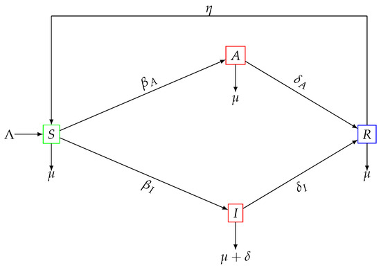
Figure 1. Flow diagram for SIARS-type mathematical model (1).

The dynamics of the subpopulations presented in the system (1) are based on implicitly assuming a homogeneous mixture in the total population $N_T=S\left(t\right)+I\left(t\right)+A\left(t\right)+R\left(t\right)$, and the application of the law of mass action [35]. Here, we consider the force infection as the linear combination $\left({\beta }_{I}I\left(t\right)+{\beta }_{A}A\left(t\right)\right),$ and if the mortality rate is $\mu ,$ then the probability that a person survives in the period $[t-\tau ,t]$ is given by $e^{-\mu \tau }$. Consequently, the number of individuals who survive in the latent period is given by $\left({\beta }_{I}I(t-\tau )+{\beta }_{A}A(t-\tau )\right)S(t-\tau )e^{-\mu \tau }$. Moreover, the variation of ${\displaystyle \frac{dS\left(t\right)}{dt}}$, is given by the number of new susceptible people that enter the system minus the proportion of susceptibles that have been infected by having contact with infectious agents at a rate ${\beta }_I$, or with asymptomatic infected people $A\left(t\right)$, at a rate ${\beta }_A$, that is, $\left({\beta }_{I}I\left(t\right)+{\beta }_{A}A\left(t\right)\right)S\left(t\right)$. It should also be noted that recovered individuals become susceptible again at a rate $\eta$ and that susceptible individuals may die naturally at a rate $\mu$. In this way, the first equation of the model is obtained. The variations ${\displaystyle \frac{dI\left(t\right)}{dt}}$ and ${\displaystyle \frac{dA\left(t\right)}{dt}}$ consist of individuals that remained in the latency stage for a certain time $\tau$. A proportion a of individuals infected and asymptomatic go into the asymptomatic class $A\left(t\right)$, that is,

$$a\left[{\beta }_{I}S(t-\tau )I(t-\tau )+{\beta }_{A}S(t-\tau )A(t-\tau )\right]e^{-\mu \tau }.$$

The other proportion of latent individuals develop symptoms and enter the class of infected $I\left(t\right)$ that is, $(1-a)\left[{\beta }_{I}S(t-\tau )I(t-\tau )+{\beta }_{A}S(t-\tau )A(t-\tau )\right]e^{-\mu \tau }$. Now, the population in the asymptomatic class $A\left(t\right)$ transits at a rate ${\delta }_A$ to the recovered class $R\left(t\right)$, that is, ${\delta }_{A}A\left(t\right).$ Similarly, infected persons with symptoms $I\left(t\right)$ can move to the recovered class R at a rate ${\delta }_I$, that is, ${\delta }_{I}I\left(t\right)$, or those who die from the virus at a rate $\delta$, that is, $\delta I\left(t\right)$. This allows us to deduce the second and third equations of the model. Finally, the variation ${\displaystyle \frac{dR\left(t\right)}{dt}}$, is nothing more than the inflow of the factors ${\delta }_{A}A\left(t\right)$ and ${\delta }_{I}I\left(t\right)$. The outflow is composed of the recovered people who become again susceptible $S\left(t\right)$ at a rate $\eta$ and those who die naturally at a rate $\mu$. Then, the outflow is given as the factors $(\eta +\mu )R\left(t\right)$. Thus, the fourth equation of the model is obtained. Table 1 lists the specifications of each of the mentioned parameters.

Table 1. Parameters used in the COVID-19 model.

Parameter	Symbol
Latency period	$\tau$
Recruitment rate	$\mathsf{\Lambda }$
Recovery rate	$\eta$
Transmission Rate between I and S	${\beta }_I$
Transmission Rate between A and S	${\beta }_A$
Recovery rate between I and R	${\delta }_I$
Recovery rate between A and R	${\delta }_A$
Death rate from the virus	$\delta$
Natural death rate	$\mu$
Proportion	a

Positive Solutions of System (1)

Applying the basic theory for the existence and uniqueness of solutions of ordinary differential equations given in [40,41], it is concluded that the solution of model (1) with its initial conditions exists and is unique in $[0,\infty ).$

One of the characteristics of population models is that the solutions must have positive values at all times. In this direction, the model represented by (1) is a biological system that models the transmission of SARS-CoV-2 between humans. Therefore, it is necessary to analyze if the solutions are positive and bounded in some domain. The results below guarantee these important properties.

Theorem 1. 

The solution of system (1) is positive in $[0,+\infty )$.

Proof. 

We use the method of steps to demonstrate the positivity of the variables I and A. Indeed, for the interval $t\in (0,\tau ],$ it follows from the second equation of (1) that ${\displaystyle \frac{dI\left(t\right)}{dt}}\ge -(\mu +{\delta }_I+\delta )I\left(t\right),$ i.e., $I\left(t\right)\ge 0$ in this interval. In the same way, $A\left(t\right)\ge 0,$ with $0<t\le \tau .$ This implies that from the fourth equation of system (1), it follows that $R\left(t\right)\ge 0$ for all $t\in (0,\tau ].$ Thus, if there exists a $t_0\in (0,\tau ]$ such that $\dot{S}\left(t_0\right)\le 0$, $S\left(t_0\right)=0$ and $S\left(t\right)>0$ for $t\in [0,t_0),$ then from the first equation of system (1) one obtains that $0\ge \dot{S}\left(t_0\right)=\mathsf{\Lambda }+\eta R\left(t_0\right),$ which is a contradiction. Therefore, $S\left(t\right)\ge 0$ for $t\in (0,\tau ].$ The previous reasonings can be applied again in the interval $t\in (\tau ,2\tau ]$ to deduce that the model variables remain positive. In this way, it is extended to any interval of the form $t\in (n\tau ,(n+1\left)\tau \right]$ with $n=2,3,\cdots$ to include all positive times. □

It is important to prove that system (1) has bounded solutions, as it will give us important information about the behavior over time of the epidemiological model. It will show us the ability of the system to avoid uncontrolled growth of the subpopulations S, I, A, and R. When it is proven that the system solutions are bounded, it means that the variables involved in the model remain within reasonable and realistic limits as time evolves. Bounding the solutions of the model is essential to ensuring the stability of the model over time. To prove that system (1) is bounded, we start by defining the function $\rho \left(t\right)$ given by

$$\begin{array}{cc}\hfill \rho \left(t\right)& =S\left(t\right)+A\left(t\right)+I\left(t\right)+R\left(t\right)+{\int }_{t-\tau }^{t}S\left(\theta \right)[{\beta }_{I}I\left(\theta \right)+{\beta }_{A}A\left(\theta \right)]e^{-(t-\theta )\mu }d\theta \hfill \\ \hfill & =S\left(t\right)+A\left(t\right)+I\left(t\right)+R\left(t\right)+e^{-\mu t}{\int }_{t-\tau }^{t}S\left(\theta \right)[{\beta }_{I}I\left(\theta \right)+{\beta }_{A}A\left(\theta \right)]e^{-\theta \mu }d\theta .\hfill \end{array}$$

Next, we derive $\rho \left(t\right)$ with respect to time

$$\begin{array}{cc}\hfill {\displaystyle \frac{d\rho \left(t\right)}{dt}}& ={\displaystyle \frac{dS\left(t\right)}{dt}}+{\displaystyle \frac{dI\left(t\right)}{dt}}+{\displaystyle \frac{dA\left(t\right)}{dt}}+{\displaystyle \frac{dR\left(t\right)}{dt}}-\mu e^{-t\mu }{\int }_{t-\tau }^{t}S\left(\theta \right)[{\beta }_{I}I\left(\theta \right)+{\beta }_{A}A\left(\theta \right)]e^{\theta \mu }d\theta \hfill \\ & +e^{-\mu t}S[{\beta }_{I}I\left(t\right)+{\beta }_{A}A\left(t\right)]e^{\mu t}-e^{-\mu t}S(t-\tau )[{\beta }_{I}I(t-\tau )+{\beta }_{A}A(t-\tau )]e^{\mu (t-\tau )}.\hfill \end{array}$$

Thus, one obtains

$$\begin{array}{cc}\hfill {\displaystyle \frac{d\rho \left(t\right)}{dt}}& =\mathsf{\Lambda }-\mu S-\delta I\left(t\right)-\mu I\left(t\right)-\mu A\left(t\right)\hfill \\ & -\mu R\left(t\right)-\mu {\int }_{t-\tau }^{t}S\left(\theta \right)[{\beta }_{I}I\left(\theta \right)+{\beta }_{A}A\left(\theta \right)]e^{-(t-\theta )\mu }d\theta \hfill \\ & \le \mathsf{\Lambda }-\mu \rho \left(t\right).\hfill \end{array}$$

Moreover, one obtains

$$\begin{array}{c}\hfill \rho \left(t\right)\le e^{-\mu t}\rho \left(0\right)+{\displaystyle \frac{\mathsf{\Lambda }}{\mu }}\left(1-e^{-\mu t}\right),\end{array}$$

Therefore,

$$\begin{array}{c}\hfill \rho \left(t\right)\le max\left\{\rho \left(0\right),{\displaystyle \frac{\mathsf{\Lambda }}{\mu }}\right\},\end{array}$$

holds for all $t\ge 0.$ Thus, with the positivity of the solutions and the boundedness of the total population, we can define the feasible region of model (1) as

$$\begin{array}{cc}\hfill \Sigma =\{\left(S\left(t\right),I\left(t\right),A\left(t\right),R\left(t\right)\right)& /0\le S\left(t\right)+A\left(t\right)+I\left(t\right)+R\left(t\right)\le {\displaystyle \frac{\mathsf{\Lambda }}{\mu }},\hfill \\ & S\left(t\right)>0,A\left(t\right)\ge 0,I\left(t\right)\ge 0,R\left(t\right)\ge 0,t\in [0,\infty )\},\hfill \end{array}$$

(3)

which is a compact set and is positively invariant of system (1).

3. Stability Analysis of the Model in the Disease-Free Equilibrium Point

From model (1), we can see that this system has a free disease steady state given by

$$\begin{array}{c}\hfill F^0=\left(S^0,I^0,A^0,R^0\right)=\left({\displaystyle \frac{\mathsf{\Lambda }}{\mu }},0,0,0\right).\end{array}$$

(4)

Related to this equilibrium point, there is one threshold associated with the epidemiological model (1) called the basic reproduction number, which is denoted by ${\mathcal{R}}_0$. This is defined as the expected number of infections that are produced by a typical infected individual in a fully susceptible population throughout the course of the disease outbreak. To determine the basic reproductive number, we use the next-generation matrix methodology given in [42]. For the case when $\tau =0,$ the terms of infection and viral production in the model, matrices $\mathbf{F}$ and $\mathbf{V}$ are given by

$$\begin{array}{c}\hfill \mathbf{F}=\left[\begin{array}{cc}\left(1-a\right){\displaystyle \frac{\mathsf{\Lambda }}{\mu }}{\beta }_I& \left(1-a\right){\displaystyle \frac{\mathsf{\Lambda }}{\mu }}{\beta }_A\\ a{\displaystyle \frac{\mathsf{\Lambda }}{\mu }}{\beta }_I& a{\displaystyle \frac{\mathsf{\Lambda }}{\mu }}{\beta }_A\end{array}\right],\mathbf{V}=\left[\begin{array}{cc}\mu +{\delta }_I+\delta & 0\\ 0& \mu +{\delta }_A\end{array}\right],\end{array}$$

where $\mathbf{F}$ is the infection matrix and $\mathbf{V}$ is the transition matrix obtained from model (1) and evaluated at the infection-free steady-state $F^0.$ The next generation matrix given by

$$\begin{array}{c}\hfill \mathbf{F}{\mathbf{V}}^{-1}=\left[\begin{array}{cc}{\displaystyle \frac{\left(1-a\right){\beta }_I\mathsf{\Lambda }}{\mu \left(\mu +{\delta }_I+\delta \right)}}& {\displaystyle \frac{\left(1-a\right){\beta }_A\mathsf{\Lambda }}{\mu \left(\mu +{\delta }_A\right)}}\\ {\displaystyle \frac{a{\beta }_I\mathsf{\Lambda }}{\mu \left(\mu +{\delta }_I+\delta \right)}}& {\displaystyle \frac{a{\beta }_A\mathsf{\Lambda }}{\mu \left(\mu +{\delta }_A\right)}}\end{array}\right].\end{array}$$

The characteristic polynomial of matrix $\mathbf{F}{\mathbf{V}}^{-1}$ is computed as

$$\begin{array}{c}\hfill P\left(x\right)=x^2-{\displaystyle \frac{\mathsf{\Lambda }\left(a{\beta }_A\delta -a\mu {\beta }_I+a{\beta }_A\mu -a{\beta }_I{\delta }_A+a{\beta }_A{\delta }_I+\mu {\beta }_I+{\beta }_I{\delta }_A\right)x}{\mu \left(\mu +{\delta }_I+\delta \right)\left(\mu +{\delta }_A\right)}}.\end{array}$$

Thus, ${\mathcal{R}}_0$ is given by

$$\begin{array}{cc}\hfill {\mathcal{R}}_0& ={\displaystyle \frac{\mathsf{\Lambda }\left(a{\beta }_A\delta -a\mu {\beta }_I+a{\beta }_A\mu -a{\beta }_I{\delta }_A+a{\beta }_A{\delta }_I+\mu {\beta }_I+{\beta }_I{\delta }_A\right)}{\mu \left(\mu +{\delta }_A\right)\left(\mu +{\delta }_I+\delta \right)}}\hfill \\ & ={\displaystyle \frac{\mathsf{\Lambda }(1-a){\beta }_I}{\mu (\mu +{\delta }_I+\delta )}}+{\displaystyle \frac{\mathsf{\Lambda }{\beta }_{A}a}{\mu (\mu +{\delta }_A)}}.\hfill \end{array}$$

So, we obtain the next result

Theorem 2. 

Let $\tau =0.$. For ${\mathcal{R}}_0<1,$ the disease-free equilibrium state point $F^0$ of model (1) and given in (4) is locally asymptotically stable, and if ${\mathcal{R}}_0>1$ then it is unstable.

Proof. 

The theorem is proved using Theorem 2 given in [42]. □

Now, we can analyze the overall behavior of the solution of model (1) around the disease-free point for $\tau =0.$ For this, we use the following Lyapunov function

$$\begin{array}{c}\hfill {\mathcal{V}}_{F^0}\left(X\left(t\right)\right)={\beta }_I\left(\mu +{\delta }_A\right)I\left(t\right)+{\beta }_A\left(\mu +\delta +{\delta }_I\right)A\left(t\right),\end{array}$$

(5)

where $X\left(t\right)=\left(S\right(t),I(t),A(t),R(t\left)\right).$ This function satisfies

$$\begin{array}{cc}\hfill & {\mathcal{V}}_{F^0}\left(F^0\right)=0,\hfill \\ \hfill & {\mathcal{V}}_{F^0}\left(X\left(t\right)\right)>0,\mathrm{for}\mathrm{all}X\left(t\right)\ne F^0,\hfill \\ \hfill & {\mathcal{V}}_{F^0}\left(X\left(t\right)\right)\to \infty ,\mathrm{as}∥X∥\to \infty .\mathrm{Therefore},{\mathcal{V}}_{F^0}\left(X\left(t\right)\right)\mathrm{is}\mathrm{Radially}\mathrm{unbounded}.\hfill \end{array}$$

(6)

After performing the time derivative of ${\mathcal{V}}_{F^0}$ through the solutions of the system (1) and some algebraic calculations it is obtained that

$$\begin{array}{cc}\hfill {\displaystyle \frac{d{\mathcal{V}}_{F^0}\left(X\left(t\right)\right)}{dt}}& =\left(\mu +{\delta }_A\right)\left(\mu +\delta +{\delta }_I\right)\left({\displaystyle \frac{{\beta }_I(1-a)S\left(t\right)}{\mu +\delta +{\delta }_I}}+{\displaystyle \frac{{\beta }_{A}aS\left(t\right)}{\mu +{\delta }_A}}-1\right)\left({\beta }_{I}I\left(t\right)+{\beta }_{A}A\left(t\right)\right)\hfill \\ & \le \left(\mu +{\delta }_A\right)\left(\mu +\delta +{\delta }_I\right)\left({\displaystyle \frac{{\beta }_I(1-a)\mathsf{\Lambda }}{\mu (\mu +\delta +{\delta }_I)}}+{\displaystyle \frac{{\beta }_{A}a\mathsf{\Lambda }}{\mu (\mu +{\delta }_A)}}-1\right)\left({\beta }_{I}I\left(t\right)+{\beta }_{A}A\left(t\right)\right)\hfill \\ & =\left(\mu +{\delta }_A\right)\left(\mu +\delta +{\delta }_I\right)\left({\mathcal{R}}_0-1\right)\left({\beta }_{I}I\left(t\right)+{\beta }_{A}A\left(t\right)\right).\hfill \end{array}$$

(7)

Therefore, when ${\mathcal{R}}_0<1$, we have that ${\displaystyle \frac{d{\mathcal{V}}_{F^0}\left(X\left(t\right)\right)}{dt}}\le 0.$ But, if ${\mathcal{R}}_0=1,$ then ${\displaystyle \frac{d{\mathcal{V}}_{F^0}\left(X\left(t\right)\right)}{dt}}=0,$ and $I=0, A=0.$ Consequently, the singleton given by $\left\{F^0\right\}$ is the largest invariant set contained in the set $\left\{(S,I,A,R)/{\dot{\mathcal{V}}}_{F^0}(S,I,A,R)=0\right\}$. Applying the invariant set theorem, each trajectory in space $\Sigma$ tends to the point $F^0$ when $t\to \infty ,$ that is, the equilibrium point $F^0$ is locally stable, which implies that it is globally asymptotically stable. Thus, we arrive at the following result:

Theorem 3. 

For $\tau =0,$ and ${\mathcal{R}}_0<1,$ the equilibrium point $F^0$ given in (4) of model (1) is globally asymptotically stable.

Next, for the case $\tau >0,$ we define the following number

$$\begin{array}{c}\hfill {\mathcal{R}}_0^D={\mathcal{R}}_0^I+{\mathcal{R}}_0^A\end{array}$$

(8)

where

$$\begin{array}{c}\hfill {\mathcal{R}}_0^I={\displaystyle \frac{\mathsf{\Lambda }{e}^{-\mu \tau }}{\mu }}{\displaystyle \frac{(1-a){\beta }_I}{\left(\delta +\mu +{\delta }_I\right)}},{\mathcal{R}}_0^A={\displaystyle \frac{\mathsf{\Lambda }{e}^{-\mu \tau }}{\mu }}{\displaystyle \frac{a{\beta }_A}{\left(\mu +{\delta }_A\right)}}.\end{array}$$

(9)

The value of the threshold parameter ${\mathcal{R}}_0^D$ makes it possible to predict whether the disease can be eliminated or whether it will continue to be endemic. Thus, if ${\mathcal{R}}_0^D<1,$ the transmission of disease can be eradicated with the assumption that the initial sizes of the subpopulations of model (1) are in an attractive neighborhood of the $F^0$. The following theorem guarantees the above statement.

Theorem 4. 

When ${\mathcal{R}}_0^D<1$ and $\tau >0,$ the disease-free equilibrium point of system (1) and given in (4) is locally asymptotically stable, and unstable if ${\mathcal{R}}_0^D>1.$

Proof. 

Obtaining the characteristic equation of model (1) is calculated as the determinant of the following matrix evaluated at the disease-free point given in (4),

$$\begin{array}{c}\hfill \left|\begin{array}{cccc}-\mu -\lambda & -{\displaystyle \frac{{\beta }_I\mathsf{\Lambda }}{\mu }}& -{\displaystyle \frac{{\beta }_A\mathsf{\Lambda }}{\mu }}& \eta \\ 0& -\mu -{\delta }_I-\delta +e^{-\lambda \tau }K-\lambda & {\displaystyle \frac{{\mathrm{e}}^{-\lambda \tau }\left(1-a\right)\mathsf{\Lambda }{\beta }_A{\mathrm{e}}^{-\mu \tau }}{\mu }}& 0\\ 0& {\displaystyle \frac{{\mathrm{e}}^{-\lambda \tau }a{\beta }_I\mathsf{\Lambda }{\mathrm{e}}^{-\mu \tau }}{\mu }}& -\mu -{\delta }_A+e^{-\lambda \tau }T-\lambda & 0\\ 0& {\delta }_I& {\delta }_A& -\eta -\mu -\lambda \end{array}\right|=0,\end{array}$$

with

$$\begin{array}{c}\hfill K={\displaystyle \frac{\left(1-a\right){\mathrm{e}}^{-\mu \tau }\mathsf{\Lambda }}{\mu }}{\beta }_I,T={\displaystyle \frac{a{\mathrm{e}}^{-\mu \tau }\mathsf{\Lambda }}{\mu }}{\beta }_A.\end{array}$$

Thus, one obtains two negative roots ${\lambda }_1=-\mu ,{\lambda }_2=-\eta -\mu .$ The other roots can be found in the following transcendental equation

$$\begin{array}{cc}\hfill \mathsf{\Lambda }{\mathrm{e}}^{-\lambda \tau }{\mathrm{e}}^{-\mu \tau }a{\beta }_I{\delta }_A& +{\mathrm{e}}^{-\lambda \tau }a{\beta }_I\mathsf{\Lambda }{\mathrm{e}}^{-\mu \tau }\lambda +\mathsf{\Lambda }{\mathrm{e}}^{-\lambda \tau }{\mathrm{e}}^{-\mu \tau }a\mu {\beta }_I-\mathsf{\Lambda }{\mathrm{e}}^{-\lambda \tau }{\mathrm{e}}^{-\mu \tau }a{\beta }_A{\delta }_I\hfill \\ & -\mathsf{\Lambda }{\mathrm{e}}^{-\lambda \tau }{\mathrm{e}}^{-\mu \tau }a\delta {\beta }_A-{\mathrm{e}}^{-\lambda \tau }a{\beta }_A\mathsf{\Lambda }{\mathrm{e}}^{-\mu \tau }\lambda -\mathsf{\Lambda }{\mathrm{e}}^{-\lambda \tau }{\mathrm{e}}^{-\mu \tau }a\mu {\beta }_A\hfill \\ & -\mathsf{\Lambda }{\mathrm{e}}^{-\lambda \tau }{\mathrm{e}}^{-\mu \tau }{\beta }_I{\delta }_A-{\mathrm{e}}^{-\lambda \tau }\mathsf{\Lambda }{\beta }_I{\mathrm{e}}^{-\mu \tau }\lambda -\mathsf{\Lambda }{\mathrm{e}}^{-\lambda \tau }{\mathrm{e}}^{-\mu \tau }\mu {\beta }_I\hfill \\ & +\mu {\delta }_I{\delta }_A+{\delta }_I\lambda \mu +{\mu }^A{\delta }_I+\delta \mu {\delta }_A+{\delta }_2\lambda \mu +{\mu }^A{\delta }_A\hfill \\ & +\delta \lambda \mu +\delta {\mu }^A+{\lambda }^A\mu +2\lambda {\mu }^A+{\mu }^3=0.\hfill \end{array}$$

(10)

After performing some algebraic manipulations, we define

$$\begin{array}{cc}\hfill \mathcal{F}\left(\lambda \right)=& \left(a{\beta }_I-a{\beta }_A-{\beta }_I\right){\mathrm{e}}^{-\mu \tau }{\mathrm{e}}^{-\lambda \tau }\lambda \mathsf{\Lambda }\hfill \\ & +\left(-a{\beta }_A\left({\delta }_I+\mu +\delta \right)-(1-a){\beta }_I\left({\delta }_A+\mu \right)\right){\mathrm{e}}^{-\mu \tau }{\mathrm{e}}^{-\lambda \tau }\mathsf{\Lambda }\hfill \\ & +{\lambda }^2\mu +\left(\delta \mu +2{\mu }^2+{\delta }_I\mu +{\delta }_A\mu \right)\lambda +(\delta +\mu +{\delta }_I)({\delta }_A+\mu )\mu \hfill \\ & =-\left((1-a){\beta }_I+a{\beta }_A\right){\mathrm{e}}^{-\mu \tau }{\mathrm{e}}^{-\lambda \tau }\lambda \mathsf{\Lambda }\hfill \\ & +(\delta +\mu +{\delta }_I)({\delta }_A+\mu )\mu \left(-{\mathcal{R}}_0^D{e}^{-\lambda \tau }+1\right)\hfill \\ & +{\lambda }^2\mu +\left(\delta \mu +2{\mu }^2+{\delta }_I\mu +{\delta }_A\mu \right)\lambda \hfill \\ & =-C_1{\mathrm{e}}^{-\lambda \tau }\lambda +C_2\left(-{\mathcal{R}}_0^D{e}^{-\lambda \tau }+1\right)+{\lambda }^2\mu +C_3\lambda ,\hfill \end{array}$$

(11)

where $C_1=-\left((1-a){\beta }_I+a{\beta }_A\right){\mathrm{e}}^{-\mu \tau }\mathsf{\Lambda }<0,$ $C_2=(\delta +\mu +{\delta }_I)({\delta }_A+\mu )\mu >0,$ $C_3=\mu \left(\delta +\mu +{\delta }_I+{\delta }_A+\mu \right)>0.$ Thus, if ${\mathcal{R}}_0^D>1$ for $\lambda \in \mathbf{R}$, one obtains

$$\begin{array}{c}\hfill \mathcal{F}\left(0\right)=C_2\left(1-{\mathcal{R}}_0^D\right)<0,\end{array}$$

and $\underset{\lambda \to \infty }{lim}\mathcal{F}\left(\lambda \right)=+\infty .$ This implies that $\mathcal{F}\left(\lambda \right)=0$ has a positive real root, when ${\mathcal{R}}_0>1,$ i.e., (4) is unstable. Now, for the case $\lambda \in \mathbf{C}$ and ${\mathcal{R}}_0^D<1,$ then

$$\begin{array}{c}\hfill \mathcal{F}\left(0\right)=C_2\left(1-{\mathcal{R}}_0^D\right)>0,\end{array}$$

i.e., the Equation (11) has no nonnegative real roots. If it is not true, there exists a $i\omega \in \mathbf{C}$ with $\omega >0$ such that in the Equation (11) it holds that

$$\begin{array}{c}\hfill -C_1\left(cos\left(\omega \tau \right)-isin\left(\omega \tau \right)\right)i\omega +C_2\left(-{\mathcal{R}}_0^D\left(cos\left(\omega \tau \right)-isin\left(\omega \tau \right)\right)+1\right)-{\omega }^2\mu +C_{3}i\omega =0.\end{array}$$

Thus, identifying the real and complex part, we have

$$\begin{array}{cc}\hfill & C_{1}sin\left(\omega \tau \right)\omega -C_2{\mathcal{R}}_0^{D}cos\left(\omega \tau \right)={\omega }^2\mu -C_2,\hfill \\ \hfill & C_{1}cos\left(\omega \tau \right)\omega +C_2{\mathcal{R}}_0^{D}sin\left(\omega \tau \right)=-C_3\omega .\hfill \end{array}$$

In the above equations, if we square and add, one obtains that

$$\begin{array}{c}\hfill {\mu }^2{z}^2+z\left(-2\mu C_2-{C_1}^2+{C_3}^2\right)+{C_2}^2\left(1-{\left({\mathcal{R}}_0^D\right)}^2\right)=0,\end{array}$$

(12)

where $z={\omega }^2.$ Since ${\mathcal{R}}_0^D<1,$ then ${C_2}^2\left(1-{\left({\mathcal{R}}_0^D\right)}^2\right)>0.$ Next, the positivity of the expression $\left(-2\mu C_2-{C_1}^2+{C_3}^2\right)$ follows from the fact that

$$\begin{array}{cc}\hfill & {\left({(\mu +\delta +{\delta }_I)}^{2}a{\beta }_A-{(\mu +{\delta }_A)}^2(1-a){\beta }_I\right)}^2\hfill \\ & +2(1-a){\beta }_{I}a{\beta }_A(\mu +\delta +{\delta }_I)(\mu +{\delta }_A)\left({(\mu +\delta +{\delta }_I)}^2+{(\mu +{\delta }_A)}^2\right)>0,\hfill \end{array}$$

(13)

and ${\mathcal{R}}_0^D<1.$ Indeed, after performing some algebraic manipulations, one obtains that

$$\begin{array}{c}\hfill {\left({\displaystyle \frac{(1-a){\beta }_I}{\left(\delta +\mu +{\delta }_I\right)}}+{\displaystyle \frac{a{\beta }_A}{\left(\mu +{\delta }_A\right)}}\right)}^2>{\displaystyle \frac{{\left((1-a){\beta }_I+a{\beta }_A\right)}^2}{{\left(\delta +\mu +{\delta }_I\right)}^2+{\left(\mu +{\delta }_A\right)}^2}}.\end{array}$$

(14)

Thus,

$$\begin{array}{c}\hfill {\left({\mathcal{R}}_0^D\right)}^2={\left({\displaystyle \frac{(1-a){\beta }_I}{\left(\delta +\mu +{\delta }_I\right)}}+{\displaystyle \frac{a{\beta }_A}{\left(\mu +{\delta }_A\right)}}\right)}^2{\displaystyle \frac{{\mathsf{\Lambda }}^2{e}^{-2\mu \tau }}{{\mu }^2}}>{\displaystyle \frac{{\left((1-a){\beta }_I+a{\beta }_A\right)}^2}{{\left(\delta +\mu +{\delta }_I\right)}^2+{\left(\mu +{\delta }_A\right)}^2}}{\displaystyle \frac{{\mathsf{\Lambda }}^2{e}^{-2\mu \tau }}{{\mu }^2}}.\end{array}$$

Since ${\mathcal{R}}_0^D<1,$ one gets

$$\begin{array}{c}\hfill {\left(\delta +\mu +{\delta }_I\right)}^2+{\left(\mu +{\delta }_A\right)}^2-{\left((1-a){\beta }_I+a{\beta }_A\right)}^2{\displaystyle \frac{{\mathsf{\Lambda }}^2{e}^{-2\mu \tau }}{{\mu }^2}}>0.\end{array}$$

(15)

Therefore, using inequality (15) it follows that

$$\begin{array}{cc}\hfill -2\mu C_2-{C_1}^2+{C_3}^2& ={\mu }^2({\left(\delta +\mu +{\delta }_I\right)}^2+{\left(\mu +{\delta }_A\right)}^2{\mu }^2\hfill \\ & -{\left((1-a){\beta }_I+a{\beta }_A\right)}^2{\mathsf{\Lambda }}^2{e}^{-2\mu \tau }>0.\hfill \end{array}$$

Because the coefficients in Equation (12) are all positive, it has no positive root $z.$ This is contradicted by the fact that $z={\omega }^2.$ In this way, Equation (11) has no pure imaginary root. Then, it is true that for all $\tau >0,$ it has only roots that have negative real parts. We concluded that $F^0$ is locally asymptotically stable. □

Now, if the disease eradication is independent of the initial conditions of the subpopulations, then, for ${\mathcal{R}}_0^D<1,$ the $F^0$ is globally asymptotically stable (GAS). This condition is demonstrated below.

Theorem 5. 

The disease-free equilibrium point (3) of system (1) is globally asymptotically stable, while ${\mathcal{R}}_0^D\le 1$ and $\tau >0.$

Proof. 

We use a suitable Lyapunov function in order to analyze the global stability of the disease-free point. For this, we define

$$\begin{array}{cc}\hfill {\mathcal{F}}_{F^0}\left(X\left(t\right)\right)& ={\beta }_I\left(\mu +{\delta }_A\right)I\left(t\right)+{\beta }_A\left(\mu +\delta +{\delta }_I\right)A\left(t\right)\hfill \\ & +\left(\mu +{\delta }_A\right)\left(\mu +\delta +{\delta }_I\right){\displaystyle \frac{\mu }{\mathsf{\Lambda }}}{\int }_{t-\tau }^{t}S\left(\theta \right)\left({\beta }_{I}I\left(\theta \right)+{\beta }_{A}A\left(\theta \right)\right)d\theta ,\hfill \end{array}$$

(16)

where $X\left(t\right)=\left(S\left(t\right),I\left(t\right),A\left(t\right),R\left(t\right)\right).$ Next, by realizing the time derivative of ${\mathcal{F}}_{F^0}\left(X\left(t\right)\right)$ through of the solutions of model (1), and using the fact that $S\left(t\right)\in \Sigma$, one obtains that

$$\begin{array}{cc}\hfill {\displaystyle \frac{d{\mathcal{F}}_{F^0}\left(X\left(t\right)\right)}{dt}}& =e^{-\mu \tau }\left((1-a){\beta }_I(\mu +{\delta }_A)+{\beta }_A(\mu +{\delta }_I+\delta )a\right)S(t-\tau )\left({\beta }_{I}I(t-\tau )+{\beta }_{A}A(t-\tau )\right)\hfill \\ & -(\mu +{\delta }_I+\delta )(\mu +{\delta }_A)\left({\beta }_{I}I\left(t\right)+{\beta }_{A}A\left(t\right)\right)\hfill \\ & +(\mu +{\delta }_I+\delta )(\mu +{\delta }_A){\displaystyle \frac{\mu }{\mathsf{\Lambda }}}S\left(t\right)\left({\beta }_{I}I\left(t\right)+{\beta }_{A}A\left(t\right)\right)\hfill \\ & -(\mu +{\delta }_I+\delta )(\mu +{\delta }_A){\displaystyle \frac{\mu }{\mathsf{\Lambda }}}S(t-\tau )\left({\beta }_{I}I(t-\tau )+{\beta }_{A}A(t-\tau )\right)\hfill \\ & \le S(t-\tau )\left({\beta }_{I}I(t-\tau )+{\beta }_{A}A(t-\tau )\right)(\mu +{\delta }_A)(\mu +{\delta }_I+\delta ){\displaystyle \frac{\mu }{\mathsf{\Lambda }}}\ast \hfill \\ & \left[{\displaystyle \frac{\mathsf{\Lambda }}{\mu }}{\displaystyle \frac{e^{-\mu \tau }\left((1-a){\beta }_I(\mu +{\delta }_A)+{\beta }_A(\mu +{\delta }_I+\delta )a\right)}{(\mu +{\delta }_A)(\mu +{\delta }_I+\delta )}}-1\right]\hfill \\ & =S(t-\tau )\left({\beta }_{I}I(t-\tau )+{\beta }_{A}A(t-\tau )\right)(\mu +{\delta }_A)(\mu +{\delta }_I+\delta ){\displaystyle \frac{\mu }{\mathsf{\Lambda }}}\left[{\mathcal{R}}_0^D-1\right].\hfill \end{array}$$

Then, ${\displaystyle \frac{d{\mathcal{F}}_{F^0}\left(X\left(t\right)\right)}{dt}}\le 0$ if ${\mathcal{R}}_0^D\le 1,$ and ${\displaystyle \frac{d{\mathcal{F}}_{F^0}\left(X\left(t\right)\right)}{dt}}=0$ if and only if $I\left(t\right)=0,A\left(t\right)=0.$ This implies that the set

$$\begin{array}{c}\hfill \left\{X\left(t\right)\in \Sigma :{\displaystyle \frac{d{\mathcal{F}}_{F^0}\left(X\left(t\right)\right)}{dt}}=0\right\},\end{array}$$

is reduced to $\left\{F^0\right\}.$ Then, applying The Lyapunov Theorem, the disease-free equilibrium is globally asymptotically stable in $\Sigma ,$ provided that ${\mathcal{R}}_0^D<1$ and $\tau >0.$ □

4. Stability Analysis of the Model in Endemic Equilibrium Point

Now, when ${\mathcal{R}}_0^D>1$ the infection-free equilibrium point $F^0$ is unstable, that is, the infection tends to grow and the solution of system (1) converges to the endemic equilibrium point, which is denoted by

$$\begin{array}{c}\hfill E^{\ast }=\left(S^{\ast },I^{\ast },A^{\ast },R^{\ast }\right),\end{array}$$

(17)

with $S^{\ast }>0,I^{\ast }>0,A^{\ast }>0,R^{\ast }>0,$ which satisfy

$$\begin{array}{c}\hfill \mathsf{\Lambda }+\eta R^{\ast }-{\beta }_I{S}^{\ast }{I}^{\ast }-{\beta }_A{S}^{\ast }{A}^{\ast }-\mu S^{\ast }=0,\\ \hfill \\ \hfill (1-a)\left[{\beta }_I{S}^{\ast }{I}^{\ast }+{\beta }_A{S}^{\ast }{A}^{\ast }\right]e^{-\mu \tau }-(\mu +{\delta }_I+\delta )I^{\ast }=0,\\ \\ \hfill a\left[{\beta }_I{S}^{\ast }{I}^{\ast }+{\beta }_A{S}^{\ast }{A}^{\ast }\right]e^{-\mu \tau }-(\mu +{\delta }_A)A^{\ast }=0,\\ \hfill \\ \hfill {\delta }_A{A}^{\ast }+{\delta }_I{I}^{\ast }-(\eta +\mu )R^{\ast }=0.\end{array}$$

(18)

After performing some algebraic manipulations on system (18), it follows that

$$\begin{array}{cc}\hfill S^{\ast }& ={\displaystyle \frac{\delta \mu +\delta {\delta }_A+{\mu }^2+\mu {\delta }_I+\mu {\delta }_A+{\delta }_I{\delta }_A}{{\mathrm{e}}^{-\mu \tau }\left(a\delta {\beta }_A-a\mu {\beta }_I+a\mu {\beta }_A-a{\beta }_I{\delta }_A+a{\beta }_A{\delta }_I+\mu {\beta }_I+{\beta }_I{\delta }_A\right)}}={\displaystyle \frac{\mathsf{\Lambda }}{\mu {\mathcal{R}}_0^D}},\hfill \\ \hfill A^{\ast }& ={\displaystyle \frac{a\mu \left(\eta +\mu \right)\left(\mu +{\delta }_I+\delta \right)\mathsf{\Lambda }\left({\mathcal{R}}_0^D-1\right)}{\mathsf{\Theta }}},\hfill \\ \hfill R^{\ast }& ={\displaystyle \frac{\mu \left(\left(\mu (1-a)+{\delta }_A\right){\delta }_I+\left(a\delta +a\mu \right){\delta }_A\right)\mathsf{\Lambda }\left({\mathcal{R}}_0^D-1\right)}{\mathsf{\Theta }}}\hfill \\ \hfill I^{\ast }& ={\displaystyle \frac{\mu \left(\mu +{\delta }_A\right)\left(\eta +\mu \right)\left(1-a\right)\mathsf{\Lambda }\left({\mathcal{R}}_0^D-1\right)}{\mathsf{\Theta }}},\hfill \end{array}$$

(19)

with

$$\begin{array}{cc}\hfill \mathsf{\Theta }& =\mu {\mathcal{R}}_0^D\left((\mu +\eta )e^{\mu \tau }(\delta +\mu +{\delta }_I)(\mu +{\delta }_A)-\eta \left(\mu (1-a){\delta }_I+{\delta }_A({\delta }_I+a\mu +a\delta )\right)\right)\hfill \\ \hfill & >(\mu +\eta ){\mathcal{R}}_0^D\left((\mu +\eta )e^{\mu \tau }(\delta +\mu +{\delta }_I)(\mu +{\delta }_A)-\left(\mu (1-a){\delta }_I+{\delta }_A({\delta }_I+a\mu +a\delta )\right)\right)\hfill \\ \hfill & >(\mu +\eta ){\mathcal{R}}_0^D\left((\mu +\eta )e^{\mu \tau }(\delta +\mu +{\delta }_I)(\mu +{\delta }_A)-\left(\mu +{\delta }_A)({\delta }_I+a\mu +a\delta )\right)\right)>0.\hfill \end{array}$$

Thus, we establish the following proposition:

Proposition 1. 

If ${\mathcal{R}}_0^D>1$, then a unique endemic equilibrium $E^{\ast }$ exists for model (1) when $\tau \ge 0,$ and its components are given by (19).

The local analysis dynamical at the endemic point for the case $\tau >0$ is impossible due to the complexity of the characteristic polynomial, which is the determinant of the following matrix:

$$\begin{array}{c}\hfill \left[\begin{array}{cccc}-\lambda -{\mathit{A}}_{\mathit{1}}& -{\mathit{A}}_{\mathit{5}}& -{\mathit{A}}_{\mathit{6}}& \eta \\ {\mathrm{e}}^{-\lambda \tau }{\mathit{P}}_{\mathit{1}}& {\mathit{A}}_{\mathit{2}}+{\mathrm{e}}^{-\lambda \tau }{\mathit{P}}_{\mathit{2}}-\lambda & {\mathrm{e}}^{-\lambda \tau }{\mathit{P}}_{\mathit{3}}& 0\\ {\mathrm{e}}^{-\lambda \tau }{\mathit{P}}_{\mathit{4}}& {\mathrm{e}}^{-\lambda \tau }{\mathit{P}}_{\mathit{5}}& -{\mathit{A}}_{\mathit{3}}+{\mathrm{e}}^{-\lambda \tau }{\mathit{P}}_{\mathit{6}}-\lambda & 0\\ 0& {\delta }_I& {\delta }_A& -{\mathit{A}}_{\mathit{4}}-\lambda \end{array}\right]\end{array}$$

where

$$\begin{array}{cc}\hfill {\mathit{P}}_{\mathit{1}}& =\left(1-a\right)\left(A^{\ast }{\beta }_2+I^{\ast }{\beta }_1\right){\mathrm{e}}^{-\mu \tau },{\mathit{P}}_{\mathit{2}}={\displaystyle \frac{\left(1-a\right)\mathsf{\Lambda }{\beta }_1{\mathrm{e}}^{-\mu \tau }}{\mu R_0}},{\mathit{P}}_{\mathit{3}}={\displaystyle \frac{\left(1-a\right)\mathsf{\Lambda }{\beta }_2{\mathrm{e}}^{-\mu \tau }}{\mu R_0}},\hfill \\ \hfill {\mathit{A}}_{\mathit{1}}& =-A^{\ast }{\beta }_2-I^{\ast }{\beta }_1-\mu ,{\mathit{A}}_{\mathit{2}}=-\mu -{\delta }_I-\delta ,{\mathit{P}}_{\mathit{4}}=a\left(A^{\ast }{\beta }_2+I^{\ast }{\beta }_1\right){\mathrm{e}}^{-\mu \tau },\hfill \\ \hfill {\mathit{P}}_{\mathit{5}}& ={\displaystyle \frac{a\mathsf{\Lambda }{\beta }_1{\mathrm{e}}^{-\mu \tau }}{\mu R_0}},{\mathit{P}}_{\mathit{6}}={\displaystyle \frac{a\mathsf{\Lambda }{\beta }_2{\mathrm{e}}^{-\mu \tau }}{\mu R_0}},{\mathit{A}}_{\mathit{3}}=-\mu -{\delta }_A,{\mathit{A}}_{\mathit{4}}=-\eta -\mu ,{\mathit{A}}_{\mathit{5}}=-{\displaystyle \frac{{\beta }_1\mathsf{\Lambda }}{\mu R_0}},\hfill \\ \hfill {\mathit{A}}_{\mathit{6}}& =-{\displaystyle \frac{{\beta }_2\mathsf{\Lambda }}{\mu R_0}}.\hfill \end{array}$$

$$\begin{array}{cc}\hfill P\left(\lambda \right)& ={\lambda }^4+\left(\left(-P_2-P_6\right){\mathrm{e}}^{-\lambda \tau }+A_1-A_2+A_3+A_4\right){\lambda }^3\hfill \\ & +(\left(P_2{P}_6-P_3{P}_5\right){\left({\mathrm{e}}^{-\lambda \tau }\right)}^2\hfill \\ & +\left(-A_1{P}_2-A_1{P}_6+A_2{P}_6-A_3{P}_2-A_4{P}_2-A_4{P}_6+A_5{P}_1+A_6{P}_4\right){\mathrm{e}}^{-\lambda \tau }\hfill \\ & -A_1{A}_2+A_1{A}_3+A_1{A}_4-A_2{A}_3-A_2{A}_4+A_3{A}_4){\lambda }^2\hfill \\ & +\left(\right(A_1{P}_2{P}_6-A_1{P}_3{P}_5+A_4{P}_2{P}_6-A_4{P}_3{P}_5-A_5{P}_1{P}_6+A_5{P}_3{P}_4+A_6{P}_1{P}_5\hfill \\ & -A_6{P}_2{P}_4){\left({\mathrm{e}}^{-\lambda \tau }\right)}^2+(-\eta P_1{\delta }_I-\eta P_4{\delta }_A+A_1{A}_2{P}_6-A_1{A}_3{P}_2-A_1{A}_4{P}_2-A_1{A}_4{P}_6\hfill \\ & +A_2{A}_4{P}_6-A_2{A}_6{P}_4-A_3{A}_4{P}_2+A_3{A}_5{P}_1+A_4{A}_5{P}_1+A_4{A}_6{P}_4){\mathrm{e}}^{-\lambda \tau }\hfill \\ & -A_1{A}_2{A}_3-A_1{A}_2{A}_4+A_1{A}_3{A}_4-A_2{A}_3{A}_4)\lambda \hfill \\ & +(-\eta P_1{P}_5{\delta }_A+\eta P_1{P}_6{\delta }_A+\eta P_2{P}_4{\delta }_A-\eta P_3{P}_4{\delta }_I+A_1{A}_4{P}_2{P}_6-A_1{A}_4{P}_3{P}_5\hfill \\ & -A_4{A}_5{P}_1{P}_6+A_4{A}_5{P}_3{P}_4+A_4{A}_6{P}_1{P}_5-A_4{A}_6{P}_2{P}_4){\left({\mathrm{e}}^{-\lambda \tau }\right)}^2\hfill \\ & +(\eta A_2{P}_4{\delta }_A-\eta A_3{P}_1{\delta }_I+A_1{A}_2{A}_4{P}_6-A_1{A}_3{A}_4{P}_2-A_2{A}_4{A}_6{P}_4\hfill \\ & +A_3{A}_4{A}_5{P}_1){\mathrm{e}}^{-\lambda \tau }-A_1{A}_2{A}_3{A}_4.\hfill \end{array}$$

However, for the case $\eta =0$, it is possible to perform a global analysis using the Lyapunov functions. The system (1) comes as given by

$$\begin{array}{cc}\hfill {\displaystyle \frac{dS\left(t\right)}{dt}}& =\mathsf{\Lambda }-{\beta }_{I}S\left(t\right)I\left(t\right)-{\beta }_{A}S\left(t\right)A\left(t\right)-\mu S\left(t\right),\hfill \\ \hfill {\displaystyle \frac{dI\left(t\right)}{dt}}& =(1-a)\left[{\beta }_{I}S(t-\tau )I(t-\tau )+{\beta }_{A}S(t-\tau )A(t-\tau )\right]e^{-\mu \tau }-(\mu +{\delta }_I+\delta )I\left(t\right),\hfill \\ \hfill {\displaystyle \frac{dA\left(t\right)}{dt}}& =a\left[{\beta }_{I}S(t-\tau )I(t-\tau )+{\beta }_{A}S(t-\tau )A(t-\tau )\right]e^{-\mu \tau }-(\mu +{\delta }_A)A\left(t\right),\hfill \\ \hfill {\displaystyle \frac{dR\left(t\right)}{dt}}& ={\delta }_{A}A\left(t\right)+{\delta }_{I}I\left(t\right)-\mu R\left(t\right).\hfill \end{array}$$

(20)

The last equation in the above system does not affect the previous equations. Thus, we can focus on this new system

$$\begin{array}{cc}\hfill {\displaystyle \frac{dS\left(t\right)}{dt}}& =\mathsf{\Lambda }-{\beta }_{I}S\left(t\right)I\left(t\right)-{\beta }_{A}S\left(t\right)A\left(t\right)-\mu S\left(t\right),\hfill \\ \hfill {\displaystyle \frac{dI\left(t\right)}{dt}}& =(1-a)\left[{\beta }_{I}S(t-\tau )I(t-\tau )+{\beta }_{A}S(t-\tau )A(t-\tau )\right]e^{-\mu \tau }-(\mu +{\delta }_I+\delta )I\left(t\right),\hfill \\ \hfill {\displaystyle \frac{dA\left(t\right)}{dt}}& =a\left[{\beta }_{I}S(t-\tau )I(t-\tau )+{\beta }_{A}S(t-\tau )A(t-\tau )\right]e^{-\mu \tau }-(\mu +{\delta }_A)A\left(t\right),\hfill \end{array}$$

(21)

where

$$\begin{array}{cc}\hfill & \mathsf{\Lambda }=S^{\ast }P+\mu S^{\ast },\hfill \\ \hfill & (1-a)S^{\ast }P{e}^{-\mu \tau }=(\mu +{\delta }_I+\delta )I^{\ast },\hfill \\ \hfill & a{S}^{\ast }P{e}^{-\mu \tau }=(\mu +{\delta }_A)A^{\ast }.\hfill \end{array}$$

(22)

with $P={\beta }_I{I}^{\ast }+{\beta }_A{A}^{\ast }.$ The following result shows global stability under special conditions.

Theorem 6. 

If $I\left(t\right),A\left(t\right)\ge 1,{\mathcal{R}}_0^D>1,$ and $X^{\ast }=(S^{\ast },I^{\ast },A^{\ast })$ satisfies (22), then the endemic equilibrium point $X^{\ast }$ of system (21) is globally asymptotically stable.

Proof. 

First, we consider the following system

$$\begin{array}{cc}\hfill {\displaystyle \frac{dS\left(t\right)}{dt}}& =\mathsf{\Lambda }-{\beta }_{I}S\left(t\right)I\left(t\right)-{\beta }_{A}S\left(t\right)A\left(t\right)-\mu S\left(t\right),\hfill \\ \hfill {\displaystyle \frac{dI\left(t\right)}{dt}}& =(1-a)\left[{\beta }_{I}S\left(t\right)I\left(t\right)+{\beta }_{A}S\left(t\right)A\left(t\right)\right]e^{-\mu \tau }-(\mu +{\delta }_I+\delta )I\left(t\right),\hfill \\ \hfill {\displaystyle \frac{dA\left(t\right)}{dt}}& =a\left[{\beta }_{I}S\left(t\right)I\left(t\right)+{\beta }_{A}S\left(t\right)A\left(t\right)\right]e^{-\mu \tau }-(\mu +{\delta }_A)A\left(t\right),\hfill \end{array}$$

(23)

which has the same equilibrium points as the system (21), and of course, equality (22) is fulfilled, [43]. Next, we take the Lyapunov function given by

$$\begin{array}{c}\hfill {\mathcal{F}}_{X^{\ast }}\left(X\left(t\right)\right)=S^{\ast }G\left({\displaystyle \frac{S\left(t\right)}{S^{\ast }}}\right)+C_2{I}^{\ast }G\left({\displaystyle \frac{I\left(t\right)}{I^{\ast }}}\right)+C_3{A}^{\ast }G\left({\displaystyle \frac{A\left(t\right)}{A^{\ast }}}\right),\end{array}$$

(24)

where $G\left(w\right)=w-1-ln\left(w\right)$ is the Volterra function which is no negative for $w>0,$ and the constants

$$\begin{array}{c}\hfill C_2={\displaystyle \frac{I^{\ast }{\beta }_I}{(1-a)P{e}^{-\mu \tau }}},C_3={\displaystyle \frac{A^{\ast }{\beta }_A}{aP{e}^{-\mu \tau }}},P={\beta }_I{I}^{\ast }+{\beta }_A{A}^{\ast }.\end{array}$$

The system (23) can be written as ${\displaystyle \frac{dX\left(t\right)}{dt}}=F\left(X\left(t\right)\right),$ with $X\left(t\right)=\left(S\right(t),I(t),A(t\left)\right)$ and

$$\begin{array}{c}\hfill F\left(X\left(t\right)\right)=\left(\begin{array}{c}\mathsf{\Lambda }-{\beta }_{I}S\left(t\right)I\left(t\right)-{\beta }_{A}S\left(t\right)A\left(t\right)-\mu S\left(t\right)\\ (1-a)\left[{\beta }_{I}S\left(t\right)I\left(t\right)+{\beta }_{A}S\left(t\right)A\left(t\right)\right]e^{-\mu \tau }-(\mu +{\delta }_I+\delta )I\left(t\right)\\ a\left[{\beta }_{I}S\left(t\right)I\left(t\right)+{\beta }_{A}S\left(t\right)A\left(t\right)\right]e^{-\mu \tau }-(\mu +{\delta }_A)A\left(t\right)\end{array}\right)\end{array}$$

Thus, one obtains that

$$\begin{array}{cc}\hfill \nabla {\mathcal{F}}_{X^{\ast }}\left(X\left(t\right)\right)·F\left(X\left(t\right)\right)=& \left[\left(1-{\displaystyle \frac{S^{\ast }}{S\left(t\right)}}\right),C_2\left(1-{\displaystyle \frac{I^{\ast }}{I\left(t\right)}}\right),C_3\left(1-{\displaystyle \frac{A^{\ast }}{A\left(t\right)}}\right)\right]·F\left(X\left(t\right)\right)\hfill \\ \hfill =& \left(1-{\displaystyle \frac{S^{\ast }}{S\left(t\right)}}\right)\left(-\mu \left(S\left(t\right)-S^{\ast }\right)-{\beta }_{I}S\left(t\right)I\left(t\right)-{\beta }_{A}S\left(t\right)A\left(t\right)+S^{\ast }P\right)\hfill \\ \hfill +& C_2\left(1-{\displaystyle \frac{I^{\ast }}{I\left(t\right)}}\right)((1-a)S\left(t\right)\left({\beta }_{I}I\left(t\right)+{\beta }_{A}A\left(t\right)\right)e^{-\mu \tau }\hfill \\ \hfill -& {\displaystyle \frac{(1-a)e^{-\mu \tau }{S}^{\ast }PI\left(t\right)}{I^{\ast }}})\hfill \\ \hfill +& C_3\left(1-{\displaystyle \frac{A^{\ast }}{A\left(t\right)}}\right)\left(aS\left(t\right)\left({\beta }_{I}I\left(t\right)+{\beta }_{A}A\left(t\right)\right)e^{-\mu \tau }-{\displaystyle \frac{a{e}^{-\mu \tau }{S}^{\ast }PA\left(t\right)}{A^{\ast }}}\right).\hfill \end{array}$$

(25)

After performing some algebraic manipulations and using the GM-HM (geometric mean-harmonic mean) inequality we arrive at the following result:

$$\begin{array}{cc}\hfill \nabla {\mathcal{F}}_{X^{\ast }}\left(X\left(t\right)\right)·F\left(X\left(t\right)\right)& =-\mu {\displaystyle \frac{{\left(S\left(t\right)-S^{\ast }\right)}^2}{S\left(t\right)}}+S^{\ast }P\left(2-{\displaystyle \frac{S^{\ast }}{S\left(t\right)}}-{\displaystyle \frac{S\left(t\right)}{S^{\ast }}}\right)\hfill \\ & +{\displaystyle \frac{S\left(t\right)A^{\ast }{\beta }_A{I}^{\ast }{\beta }_I}{P}}\left(2-{\displaystyle \frac{I^{\ast }A\left(t\right)}{A^{\ast }I\left(t\right)}}-{\displaystyle \frac{A^{\ast }I\left(t\right)}{I^{\ast }A\left(t\right)}}\right)\le 0.\hfill \end{array}$$

(26)

Now, we calculate the time derivative of (24) through solutions of (21) in the following way:

$$\begin{array}{cc}\hfill {\displaystyle \frac{d{\mathcal{F}}_{X^{\ast }}\left(X\left(t\right)\right)}{dt}}& =\left(1-{\displaystyle \frac{S^{\ast }}{S\left(t\right)}}\right){\displaystyle \frac{dS\left(t\right)}{dt}}+C_2\left(1-{\displaystyle \frac{I^{\ast }}{I\left(t\right)}}\right){\displaystyle \frac{dI\left(t\right)}{dt}}+C_3\left(1-{\displaystyle \frac{A^{\ast }}{A\left(t\right)}}\right){\displaystyle \frac{dA\left(t\right)}{dt}}\hfill \\ & =\left(1-{\displaystyle \frac{S^{\ast }}{S\left(t\right)}}\right)\left(\mathsf{\Lambda }-{\beta }_{I}S\left(t\right)I\left(t\right)-{\beta }_{A}S\left(t\right)A\left(t\right)-\mu S\left(t\right)\right)\hfill \\ & +C_2\left(1-{\displaystyle \frac{I^{\ast }}{I\left(t\right)}}\right)((1-a)\left[{\beta }_{I}S(t-\tau )I(t-\tau )+{\beta }_{A}S(t-\tau )A(t-\tau )\right]e^{-\mu \tau }\hfill \\ & -(\mu +{\delta }_I+\delta )I\left(t\right))+C_3\left(1-{\displaystyle \frac{A^{\ast }}{A\left(t\right)}}\right)(a[{\beta }_{I}S(t-\tau )I(t-\tau )\hfill \\ & +{\beta }_{A}S(t-\tau )A(t-\tau )]e^{-\mu \tau }-(\mu +{\delta }_A)A\left(t\right))\hfill \\ & =\left(1-{\displaystyle \frac{S^{\ast }}{S\left(t\right)}}\right)\left(-\mu \left(S\left(t\right)-S^{\ast }\right)-{\beta }_{I}S\left(t\right)I\left(t\right)-{\beta }_{A}S\left(t\right)A\left(t\right)+S^{\ast }P\right)\hfill \\ & +C_2\left(1-{\displaystyle \frac{I^{\ast }}{I\left(t\right)}}\right)((1-a)S\left(t\right)\left({\beta }_{I}I\left(t\right)+{\beta }_{A}A\left(t\right)\right)e^{-\mu \tau }\hfill \\ & -{\displaystyle \frac{(1-a)e^{-\mu \tau }{S}^{\ast }PI\left(t\right)}{I^{\ast }}})\hfill \\ & +C_3\left(1-{\displaystyle \frac{A^{\ast }}{A\left(t\right)}}\right)\left(aS\left(t\right)\left({\beta }_{I}I\left(t\right)+{\beta }_{A}A\left(t\right)\right)e^{-\mu \tau }-{\displaystyle \frac{a{e}^{-\mu \tau }{S}^{\ast }PA\left(t\right)}{A^{\ast }}}\right)\hfill \\ & +C_2\left(1-{\displaystyle \frac{I^{\ast }}{I\left(t\right)}}\right)((1-a)\left[{\beta }_{I}S(t-\tau )I(t-\tau )+{\beta }_{A}S(t-\tau )A(t-\tau )\right]e^{-\mu \tau }\hfill \\ & -(1-a)S\left(t\right)\left({\beta }_{I}I\left(t\right)+{\beta }_{A}A\left(t\right)\right)e^{-\mu \tau })\hfill \\ & +C_3\left(1-{\displaystyle \frac{A^{\ast }}{A\left(t\right)}}\right)(a\left[{\beta }_{I}S(t-\tau )I(t-\tau )+{\beta }_{A}S(t-\tau )A(t-\tau )\right]e^{-\mu \tau }\hfill \\ & -aS\left(t\right)\left({\beta }_{I}I\left(t\right)+{\beta }_{A}A\left(t\right)\right)e^{-\mu \tau }).\hfill \end{array}$$

(27)

Thus, using (27), ones obtains that

$$\begin{array}{cc}\hfill {\displaystyle \frac{d{\mathcal{F}}_{X^{\ast }}\left(X\left(t\right)\right)}{dt}}=& \nabla {\mathcal{F}}_{X^{\ast }}\left(X\left(t\right)\right)·F\left(X\left(t\right)\right)\hfill \\ \hfill +& C_2\left(1-{\displaystyle \frac{I^{\ast }}{I\left(t\right)}}\right)((1-a)\left[{\beta }_{I}S(t-\tau )I(t-\tau )+{\beta }_{A}S(t-\tau )A(t-\tau )\right]e^{-\mu \tau }\hfill \\ \hfill -& (1-a)S\left(t\right)\left({\beta }_{I}I\left(t\right)+{\beta }_{A}A\left(t\right)\right)e^{-\mu \tau })\hfill \\ \hfill +& C_3\left(1-{\displaystyle \frac{A^{\ast }}{A\left(t\right)}}\right)(a\left[{\beta }_{I}S(t-\tau )I(t-\tau )+{\beta }_{A}S(t-\tau )A(t-\tau )\right]e^{-\mu \tau }\hfill \\ \hfill -& aS\left(t\right)\left({\beta }_{I}I\left(t\right)+{\beta }_{A}A\left(t\right)\right)e^{-\mu \tau }).\hfill \end{array}$$

(28)

Therefore, from (26) and (28), it follows that

$$\begin{array}{cc}\hfill {\displaystyle \frac{d{\mathcal{F}}_{X^{\ast }}\left(X\left(t\right)\right)}{dt}}=& -\mu {\displaystyle \frac{{\left(S\left(t\right)-S^{\ast }\right)}^2}{S\left(t\right)}}+S^{\ast }P\left(2-{\displaystyle \frac{S^{\ast }}{S\left(t\right)}}-{\displaystyle \frac{S\left(t\right)}{S^{\ast }}}\right)\hfill \\ \hfill +& {\displaystyle \frac{S\left(t\right)A^{\ast }{\beta }_A{I}^{\ast }{\beta }_I}{P}}\left(2-{\displaystyle \frac{I^{\ast }A\left(t\right)}{A^{\ast }I\left(t\right)}}-{\displaystyle \frac{A^{\ast }I\left(t\right)}{I^{\ast }A\left(t\right)}}\right)\hfill \\ \hfill +& \left(C_2(1-a)e^{-\mu \tau }+C_{3}a{e}^{-\mu \tau }\right)S(t-\tau )\left[{\beta }_{I}I(t-\tau )+{\beta }_{A}A(t-\tau )\right]\hfill \\ \hfill -& \left(C_2(1-a)e^{-\mu \tau }+C_{3}a{e}^{-\mu \tau }\right)S\left(t\right)\left[{\beta }_{I}I\left(t\right)+{\beta }_{A}A\left(t\right)\right]\hfill \\ \hfill -& [C_2(1-a)e^{-\mu \tau }{\displaystyle \frac{I^{\ast }}{I\left(t\right)}}+C_{3}a{e}^{-\mu \tau }{\displaystyle \frac{A^{\ast }}{A\left(t\right)}}]S(t-\tau )\left[{\beta }_{I}I(t-\tau )+{\beta }_{A}A(t-\tau )\right]\hfill \\ \hfill +& [C_2(1-a)e^{-\mu \tau }{\displaystyle \frac{I^{\ast }}{I\left(t\right)}}+C_{3}a{e}^{-\mu \tau }{\displaystyle \frac{A^{\ast }}{A\left(t\right)}}]S\left(t\right)\left[{\beta }_{I}I\left(t\right)+{\beta }_{A}A\left(t\right)\right]\hfill \\ \hfill =& -\mu {\displaystyle \frac{{\left(S\left(t\right)-S^{\ast }\right)}^2}{S\left(t\right)}}+S^{\ast }P\left(2-{\displaystyle \frac{S^{\ast }}{S\left(t\right)}}-{\displaystyle \frac{S\left(t\right)}{S^{\ast }}}\right)\hfill \\ \hfill +& {\displaystyle \frac{S\left(t\right)A^{\ast }{\beta }_A{I}^{\ast }{\beta }_I}{P}}\left(2-{\displaystyle \frac{I^{\ast }A\left(t\right)}{A^{\ast }I\left(t\right)}}-{\displaystyle \frac{A^{\ast }I\left(t\right)}{I^{\ast }A\left(t\right)}}\right)\hfill \\ \hfill +& S(t-\tau )\left[{\beta }_{I}I(t-\tau )+{\beta }_{A}A(t-\tau )\right]-S\left(t\right)\left[{\beta }_{I}I\left(t\right)+{\beta }_{A}A\left(t\right)\right]\hfill \\ \hfill -& [I^{\ast }{\beta }_I{\displaystyle \frac{I^{\ast }}{PI\left(t\right)}}+A^{\ast }{\beta }_A{\displaystyle \frac{A^{\ast }}{PA\left(t\right)}}]S(t-\tau )\left[{\beta }_{I}I(t-\tau )+{\beta }_{A}A(t-\tau )\right]\hfill \\ \hfill +& [I^{\ast }{\beta }_I{\displaystyle \frac{I^{\ast }}{PI\left(t\right)}}+A^{\ast }{\beta }_A{\displaystyle \frac{A^{\ast }}{PA\left(t\right)}}]S\left(t\right)\left[{\beta }_{I}I\left(t\right)+{\beta }_{A}A\left(t\right)\right].\hfill \end{array}$$

(29)

Finally, one obtains

$$\begin{array}{cc}\hfill {\displaystyle \frac{d{\mathcal{F}}_{X^{\ast }}\left(X\left(t\right)\right)}{dt}}=& -\mu {\displaystyle \frac{{\left(S\left(t\right)-S^{\ast }\right)}^2}{S\left(t\right)}}+S^{\ast }P\left(2-{\displaystyle \frac{S^{\ast }}{S\left(t\right)}}-{\displaystyle \frac{S\left(t\right)}{S^{\ast }}}\right)\hfill \\ \hfill +& {\displaystyle \frac{S\left(t\right)A^{\ast }{\beta }_A{I}^{\ast }{\beta }_I}{P}}\left(2-{\displaystyle \frac{I^{\ast }A\left(t\right)}{A^{\ast }I\left(t\right)}}-{\displaystyle \frac{A^{\ast }I\left(t\right)}{I^{\ast }A\left(t\right)}}\right)\hfill \\ \hfill +& H(I\left(t\right),A\left(t\right))S(t-\tau )\left({\beta }_{I}I(t-\tau )+{\beta }_{A}A(t-\tau )\right)\hfill \\ \hfill -& H(I\left(t\right),A\left(t\right))S\left(t\right)\left({\beta }_{I}I\left(t\right)+{\beta }_{A}A\left(t\right)\right),\hfill \end{array}$$

(30)

where $H(I\left(t\right),A\left(t\right))=1-[I^{\ast }{\beta }_I{\displaystyle \frac{I^{\ast }}{PI\left(t\right)}}+A^{\ast }{\beta }_A{\displaystyle \frac{A^{\ast },\ast }{PA\left(t\right)}}].$ Since $\underset{t\to \infty }{lim}I\left(t\right)=I^{\ast },\underset{t\to \infty }{lim}A\left(t\right)=A^{\ast },$ then $\underset{t\to \infty }{lim}H(I\left(t\right),A\left(t\right))=0.$ Moreover,

$$\begin{array}{c}\hfill \left|S(t-\tau )\left({\beta }_{I}I(t-\tau )+{\beta }_{A}A(t-\tau )\right)-S\left(t\right)\left({\beta }_{I}I\left(t\right)+{\beta }_{A}A\left(t\right)\right)\right|\le 2{\displaystyle \frac{{\mathsf{\Lambda }}^2}{{\mu }^2}}\left({\beta }_I+{\beta }_A\right).\end{array}$$

Accordingly, given $0<ϵ<1$, there is a $t_0$ such that for all $t>t_0$

$$\begin{array}{c}\hfill \left|H(I\left(t\right),A\left(t\right))\left[|S(t-\tau )\left({\beta }_{I}I(t-\tau )+{\beta }_{A}A(t-\tau )\right)-S\left(t\right)\left({\beta }_{I}I\left(t\right)+{\beta }_{A}A\left(t\right)\right)\right]\right|<ϵ.\end{array}$$

Consequently, ${\displaystyle \frac{d{\mathcal{F}}_{X^{\ast }}\left(X\left(t\right)\right)}{dt}}\le 0$ for $t>t_0.$ While, ${\displaystyle \frac{d{\mathcal{F}}_{X^{\ast }}\left(X\left(t\right)\right)}{dt}}=0$ if only if $X\left(t\right)=(S^{\ast },I^{\ast },A^{\ast }).$ Finally, the Lyapunov–LaSalle invariance principle implies that the endemic point $X^{\ast }=(S^{\ast },I^{\ast },A^{\ast })$ is globally asymptotically stable for system (21). □

5. Numerical Simulations

In this section, we present numerical simulations for a variety of scenarios where the theoretical results obtained in previous sections are reinforced. For most of the numerical simulations, we use the parameter values presented in Table 2. We vary the transmission rates ${\beta }_I$ and ${\beta }_A$ in order to obtain different values of the basic reproduction number ${\mathcal{R}}_0$ and for ${\mathcal{R}}_0^D$. Thus, we can provide numerical support to the theorems developed in this paper. For the numerical simulations we rely on the Matlab R2024a built-in function dde23, which is designed to numerically solve delay differential equations. This function can be implemented with different levels of accuracy to avoid negative solutions in most cases. However, in some situations, when the system of delay differential equations becomes stiff, other numerical schemes would be needed [44,45].

Table 2. Average values of the parameters used in model (1) to carry out numerical simulations.

Parameter	Symbol	Value
Latency period	$\tau$	varied ${\mathrm{year}}^{-1}$
Recovery rate	$\eta$	${\displaystyle \frac{365}{7}}$${\mathrm{year}}^{-1}$ [46]
Recovery rate between I and R	${\delta }_I$	varied
Recovery rate between A and R	${\delta }_A$	varied
Death rate	$\delta$	$\left({\displaystyle \frac{0.103}{10.4}}\right)\times 365$${\mathrm{year}}^{-1}$ [47,48]
Probability of being Asymptomatic	a	[0.2–0.8] [49,50]
Transmission rate between I and S	${\beta }_I$	varied
Transmission rate between A and S	${\beta }_A$	varied
Recruitment rate	$\mathsf{\Lambda }$	649,742 ${\mathrm{year}}^{-1}$ [51]
Natural Death Rate	$\mu$	varied (${\mathrm{year}}^{-1}$) [51]

5.1. Numerical Simulation When ${\mathcal{R}}_0^D<1$ and ${\mathcal{R}}_0>1$

For the first simulation of model (1), let us consider an initial condition far from the DFE and $\mathsf{\Lambda }=0.003\ast S\left(0\right)$. Using ${\beta }_I=9\times {10}^{-5}$, ${\beta }_A=7.0\times {10}^{-5}$ and $\tau =21$, one obtains that ${\mathcal{R}}_0^D\approx 0.984$ and ${\mathcal{R}}_0\approx 1.034$. Figure 2 shows that the solution of system (1) converges to the DFE. This result provides additional support to the global stability of the DFE whenever ${\mathcal{R}}_0^D<1$. We used initial conditions around the following point $S\left(0\right)=1000,I\left(0\right)=0.32\ast S\left(0\right),A\left(0\right)=0.27\ast S\left(0\right),R\left(0\right)=0.33\ast S\left(0\right)$ and varied them without affecting the main qualitative outcomes. Figure 3 shows the solution in the phase space using S, A and I. It is important to remark that even though ${\mathcal{R}}_0=1.034>1$, the numerical solution of model (1) converges to the DFE. Thus, it can be seen the importance of considering discrete time delays in the real world.

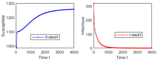
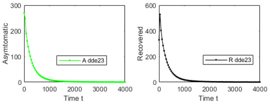
Figure 2. Numerical simulation with an initial condition far from the DFE and $\mathsf{\Lambda }=0.003\ast S\left(0\right)$. Using ${\beta }_I=9\times {10}^{-5}$, ${\beta }_A=7.0\times {10}^{-5}$ and $\tau =21$, one obtains that ${\mathcal{R}}_0^D\approx 0.984$. The plot shows the trajectory of each one of the subpopulations.

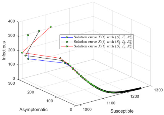
Figure 3. Numerical simulation with an initial condition far from the DFE and $\mathsf{\Lambda }=0.003\ast S\left(0\right)$. Using ${\beta }_I=9\times {10}^{-5}$, ${\beta }_A=7.0\times {10}^{-5}$ and $\tau =21$, one obtains that ${\mathcal{R}}_0^D\approx 0.984$. The plot shows the solution in the phase space using S, A and I.

5.2. Numerical Simulation When ${\mathcal{R}}_0^D>1$ and ${\mathcal{R}}_0>1$

For the second simulation of model (1), let us consider an initial condition far from the endemic equilibrium point $E^{\ast }=(S^{\ast },I^{\ast },A^{\ast },R^{\ast })$ (close to the DFE) and $\mathsf{\Lambda }=0.003\ast S\left(0\right)$. Using ${\beta }_I=9.4\times {10}^{-5}$, ${\beta }_A=7.0\times {10}^{-5}$, $\eta \ne 0$, and $\tau =1$, one obtains that ${\mathcal{R}}_0^D\approx 1.054$. Figure 4 shows that the solution of delayed system (1) converges to the endemic equilibrium point $E^{\ast }=(S^{\ast },I^{\ast },A^{\ast },R^{\ast })=(1.201\times {10}^3,4.497,6.260)$. This result provides additional support to the global stability of the endemic equilibrium point $E^{\ast }=(S^{\ast },I^{\ast },A^{\ast },R^{\ast })$ whenever ${\mathcal{R}}_0^D>1$. Note that Theorem 6 guarantees global stability when $\eta =0$. Therefore, the numerical result shows that this condition related to $\eta$ is sufficient. We used different initial conditions around $S\left(0\right)=1000,I\left(0\right)=0.03\ast S\left(0\right),A\left(0\right)=0.02\ast S\left(0\right),R\left(0\right)=0.03\ast S\left(0\right)$. We varied them in the simulations without affecting the main qualitative outcome. Figure 5 shows the solution of delayed system (1) in the phase space and it can be seen that it converges to the endemic equilibrium point $E^{\ast }=(S^{\ast },I^{\ast },A^{\ast },R^{\ast })=(1.201\times {10}^3,4.497,6.260)$.

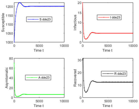
Figure 4. Numerical simulation with an initial condition far from the endemic equilibrium $E^{\ast }$ (close to DFE) and $\mathsf{\Lambda }=0.003\ast S\left(0\right)$. Using ${\beta }_I=9.4\times {10}^{-5}$ and ${\beta }_A=7.0\times {10}^{-5}$ one obtains that ${\mathcal{R}}_0^D\approx 1.054$. The solution of delayed system (1) converges to the endemic equilibrium point $E^{\ast }=(S^{\ast },I^{\ast },A^{\ast },R^{\ast })=(1.201\times {10}^3,4.497,6.260)$.

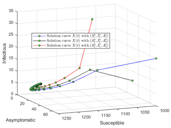
Figure 5. Numerical simulation with an initial condition far from the endemic equilibrium $E^{\ast }$ (close to DFE) and $\mathsf{\Lambda }=0.003\ast S\left(0\right)$. Using ${\beta }_I=9.4\times {10}^{-5}$ and ${\beta }_A=7.0\times {10}^{-5}$ one obtains that ${\mathcal{R}}_0^D\approx 1.054$. The solution of delayed system (1) converges to the endemic equilibrium point $E^{\ast }=(S^{\ast },I^{\ast },A^{\ast },R^{\ast })=(1.201\times {10}^3,4.497,6.260)$ regardless of the initial conditions. The plot shows the solution in the phase space using S, A, and I.

6. Discussion

In this paper, we analyzed the qualitative behavior of a mathematical model for the early phase of the COVID-19 pandemic. The constructed mathematical model is based on a system of nonlinear delay differential equations and is a SIARS-type model. The discrete-time delay was introduced in the model in order to take into account the elapsed time since an individual acquires the virus until the person is able to infect other people. In other words, the delay represents the latent stage. We investigated the qualitative dynamics of the delayed mathematical model by performing global and local stability analysis. We were able to compute the basic reproduction number ${\mathcal{R}}_0^d$, which depends on the time delay. We found that under some scenarios this threshold number determines the global stability of the disease-free equilibrium point and the unfortunate endemic equilibrium point. We made comparisons of the qualitative dynamics of the delayed model and the model without time delay, which is based on ordinary differential equations. For the global stability, we constructed two suitable Lyapunov functions, one for each one, to analyze the global stability of the equilibrium points. We established that the disease persists whenever ${\mathcal{R}}_0^d>1$ regardless of the initial conditions whenever there is life-long immunity. In the situation of waning immunity, further research is needed to explore the possibility of Hopf bifurcation or the global stability of the endemic equilibrium. On the other hand, when ${\mathcal{R}}_0^d<1$, the solution approaches the disease-free equilibrium point regardless of the initial conditions, i.e., global stable. We presented a few numerical simulations that supported the theoretical stability analysis and the methodology. One main result of this work is that there are scenarios where the solution of the model without time delay approaches the endemic steady state, but when the time delay is included in the model, then the solution approaches the disease-free steady state. Thus, the relevance of including a time delay that represents the latent stage and is more realistic than other modeling approaches can be seen. Nevertheless, one alternative to avoid the use of a time delay is the introduction of a state variable that includes the individuals in the latent stage [35,36]. However, the underlying transition from the susceptible stage to the infected or asymptomatic stages is different under these two mathematical models. There is no compelling evidence about which approach is definitively better [35]. In fact, there are models that have a combination of these modeling approaches such as the models that have gamma distributed times between stages [27,28,29,52]. Regarding backward bifurcation the mathematical model presented in this work does not have this feature. However, there are other mathematical models related to COVID-19 where backward bifurcation occurs [53,54,55,56]. The models presented in these works have different features that enable them to have backward bifurcation. For instance, in [53], the model includes a Beddington–DeAngelis-type nonlinear incidence rate and a Holling functional type II treatment term. These features give rise to two endemic equilibrium points where backward bifurcation occurs. With regard to Hopf bifurcation, there are previous mathematical models where Hopf bifurcation has been found [15,17,18,19].

As in any mathematical model, there are limitations that need to be acknowledged by the scientific community and readers. One aspect of avoiding having an explicit latent class is that the modeling of the transition from the susceptible class to the infected one requires the inclusion of survival probability, which highly depends on age. Therefore, using a model based on age-structure is more realistic despite the greater complexity of the model [57,58,59]. Nevertheless, we do not expect significant differences regarding the effect of the survival probability but the age-structure would make a great difference due to the introduction of social contact matrices that highly affect the dynamics of COVID-19 [60,61,62,63]. The proposed model does not include vaccination explicitly and this is a limitation. Other limitations that have been mentioned are the assumption of exponential transition times from the infected classes to the recovered ones or the assumption of a constant transmission rate, which is unlikely in the real world.

Finally, future research directions and open questions are the dynamics of models that include multiple time delays due to the latent stages and the time that the vaccination provides immunity or protection. In addition, the study of mathematical models for COVID-19 with distributed time delays or time-dependent delays (or even state-dependent delays) can be explored and compared with the results presented in this work. Furthermore, the consideration of different SARS-CoV-2 variants and cross-immunity provides many more research challenges.

References

- Bhadauria, A.S.; Pathak, R.; Chaudhary, M. A SIQ mathematical model on COVID-19 investigating the lockdown effect. Infect. Dis. Model. 2021, 6, 244–257. [Google Scholar] [CrossRef] [PubMed]
- Hamou, A.A.; Rasul, R.R.; Hammouch, Z.; Özdemir, N. Analysis and dynamics of a mathematical model to predict unreported cases of COVID-19 epidemic in Morocco. Comput. Appl. Math. 2022, 41, 289. [Google Scholar] [CrossRef]
- González-Parra, G.; Díaz-Rodríguez, M.; Arenas, A.J. Mathematical modeling to study the impact of immigration on the dynamics of the COVID-19 pandemic: A case study for Venezuela. Spat. Spatio-Temporal Epidemiol. 2022, 43, 100532. [Google Scholar] [CrossRef] [PubMed]
- Pham, H. On estimating the number of deaths related to Covid-19. Mathematics 2020, 8, 655. [Google Scholar] [CrossRef]
- Pinter, G.; Felde, I.; Mosavi, A.; Ghamisi, P.; Gloaguen, R. COVID-19 pandemic prediction for Hungary; a hybrid machine learning approach. Mathematics 2020, 8, 890. [Google Scholar] [CrossRef]
- Babasola, O.; Kayode, O.; Peter, O.J.; Onwuegbuche, F.C.; Oguntolu, F.A. Time-delayed modelling of the COVID-19 dynamics with a convex incidence rate. Inform. Med. Unlocked 2022, 35, 101124. [Google Scholar] [CrossRef]
- Dell’Anna, L. Solvable delay model for epidemic spreading: The case of Covid-19 in Italy. Sci. Rep. 2020, 10, 15763. [Google Scholar] [CrossRef]
- Devipriya, R.; Dhamodharavadhani, S.; Selvi, S. SEIR model FOR COVID-19 Epidemic using DELAY differential equation. J. Phys. Conf. Ser. 2021, 1767, 012005. [Google Scholar] [CrossRef]
- Ghosh, S.; Volpert, V.; Banerjee, M. An epidemic model with time delay determined by the disease duration. Mathematics 2022, 10, 2561. [Google Scholar] [CrossRef]
- Gonzalez-Parra, G. Analysis of delayed vaccination regimens: A mathematical modeling approach. Epidemiologia 2021, 2, 271–293. [Google Scholar] [CrossRef]
- Paul, S.; Lorin, E. Estimation of COVID-19 recovery and decease periods in Canada using delay model. Sci. Rep. 2021, 11, 23763. [Google Scholar] [CrossRef] [PubMed]
- Pell, B.; Johnston, M.D.; Nelson, P. A data-validated temporary immunity model of COVID-19 spread in Michigan. Math. Biosci. Eng. 2022, 19, 10122–10142. [Google Scholar] [CrossRef] [PubMed]
- Shayak, B.; Sharma, M.M.; Gaur, M.; Mishra, A.K. Impact of reproduction number on multiwave spreading dynamics of COVID-19 with temporary immunity: A mathematical model. Int. J. Infect. Dis. 2021, 104, 649–654. [Google Scholar] [CrossRef] [PubMed]
- Shayak, B.; Sharma, M.M.; Rand, R.H.; Singh, A.; Misra, A. A Delay differential equation model for the spread of COVID-19. Int. J. Eng. Res. Appl. 2020, 10, 1–13. [Google Scholar]
- Sepulveda, G.; Arenas, A.J.; González-Parra, G. Mathematical Modeling of COVID-19 dynamics under two vaccination doses and delay effects. Mathematics 2023, 11, 369. [Google Scholar] [CrossRef]
- Ng, K.Y.; Gui, M.M. COVID-19: Development of a robust mathematical model and simulation package with consideration for ageing population and time delay for control action and resusceptibility. Phys. D Nonlinear Phenom. 2020, 411, 132599. [Google Scholar] [CrossRef]
- Hassan, M.; El-Azab, T.; AlNemer, G.; Sohaly, M.; El-Metwally, H. Analysis Time-Delayed SEIR Model with Survival Rate for COVID-19 Stability and Disease Control. Mathematics 2024, 12, 3697. [Google Scholar] [CrossRef]
- Lolika, P.O.; Helikumi, M. Global stability analysis of a COVID-19 epidemic model with incubation delay. Math. Model. Control 2023, 3, 23–38. [Google Scholar] [CrossRef]
- Bugalia, S.; Tripathi, J.P.; Wang, H. Mathematical modeling of intervention and low medical resource availability with delays: Applications to COVID-19 outbreaks in Spain and Italy. Math. Biosci. Eng. 2021, 18, 5865–5920. [Google Scholar] [CrossRef]
- Gonzalez-Parra, G.; Arenas, A.J. Nonlinear Dynamics of the Introduction of a New SARS-CoV-2 Variant with Different Infectiousness. Mathematics 2021, 9, 1564. [Google Scholar] [CrossRef]
- Dobrovolny, H.M. Modeling the role of asymptomatics in infection spread with application to SARS-CoV-2. PLoS ONE 2020, 15, e0236976. [Google Scholar] [CrossRef] [PubMed]
- Dutta, S.; Dutta, P.; Samanta, G. Modelling disease transmission through asymptomatic carriers: A societal and environmental perspective. Int. J. Dyn. Control 2024, 12, 3100–3122. [Google Scholar] [CrossRef]
- González-Parra, G.; Arenas, A.J. Qualitative analysis of a mathematical model with presymptomatic individuals and two SARS-CoV-2 variants. Comput. Appl. Math. 2021, 40, 199. [Google Scholar] [CrossRef]
- Huang, L.; Xia, Y.; Qin, W. Study on SEAI Model of COVID-19 Based on Asymptomatic Infection. Axioms 2024, 13, 309. [Google Scholar] [CrossRef]
- Naz, R.; Torrisi, M. The transmission dynamics of a compartmental epidemic model for COVID-19 with the asymptomatic population via closed-form solutions. Vaccines 2022, 10, 2162. [Google Scholar] [CrossRef]
- Serhani, M.; Labbardi, H. Mathematical modeling of COVID-19 spreading with asymptomatic infected and interacting peoples. J. Appl. Math. Comput. 2021, 66, 1–20. [Google Scholar] [CrossRef]
- Conlan, A.J.; Rohani, P.; Lloyd, A.L.; Keeling, M.; Grenfell, B.T. Resolving the impact of waiting time distributions on the persistence of measles. J. R. Soc. Interface 2010, 7, 623–640. [Google Scholar] [CrossRef]
- Lloyd, A.L. Realistic distributions of infectious periods in epidemic models: Changing patterns of persistence and dynamics. Theor. Popul. Biol. 2001, 60, 59–71. [Google Scholar] [CrossRef]
- González-Parra, G.; Dobrovolny, H.M.; Aranda, D.F.; Chen-Charpentier, B.; Rojas, R.A.G. Quantifying rotavirus kinetics in the REH tumor cell line using in vitro data. Virus Res. 2018, 244, 53–63. [Google Scholar] [CrossRef]
- González-Parra, G.; Arenas, A.J. Mathematical modeling of SARS-CoV-2 omicron wave under vaccination effects. Computation 2023, 11, 36. [Google Scholar] [CrossRef]
- Kupferschmidt, K. Vaccinemakers ponder how to adapt to virus variants. Science 2021, 371, 448–449. [Google Scholar] [CrossRef] [PubMed]
- Le Page, M. Threats from new variants. New Sci. 2021, 249, 8–9. [Google Scholar] [CrossRef] [PubMed]
- van Oosterhout, C.; Hall, N.; Ly, H.; Tyler, K.M. COVID-19 evolution during the pandemic–Implications of new SARS-CoV-2 variants on disease control and public health policies. Virulence 2021, 12, 507. [Google Scholar] [CrossRef] [PubMed]
- Van den Driessche, P.; Watmough, J. Further Notes on the Basic Reproduction Number; Springer: Berlin/Heidelberg, Germany, 2008; pp. 159–178. [Google Scholar]
- Hethcote, H.W. Mathematics of infectious diseases. SIAM Rev. 2005, 42, 599–653. [Google Scholar] [CrossRef]
- Hethcote, H.W.; Van den Driessche, P. An SIS epidemic model with variable population size and a delay. J. Math. Biol. 1995, 34, 177–194. [Google Scholar] [CrossRef]
- Kuang, Y. Delay Differential Equations: With Applications in Population Dynamics; Academic Press: Cambridge, MA, USA, 1993. [Google Scholar]
- Pollock, A.M.; Lancaster, J. Asymptomatic transmission of COVID-19. BMJ 2020, 371, m4851. [Google Scholar] [CrossRef]
- Cevik, M.; Tate, M.; Lloyd, O.; Maraolo, A.E.; Schafers, J.; Ho, A. SARS-CoV-2, SARS-CoV, and MERS-CoV viral load dynamics, duration of viral shedding, and infectiousness: A systematic review and meta-analysis. Lancet Microbe 2021, 2, e13–e22. [Google Scholar] [CrossRef]
- Lambert, J.D. Computational Methods in Ordinary Differential Equations; Wiley: New York, NY, USA, 1973. [Google Scholar]
- Driver, R.D. Ordinary and Delay Differential Equations, 1st ed.; Applied Mathematical Sciences 20; Springer: New York, NY, USA, 1977. [Google Scholar]
- van den Driessche, P.; Watmough, J. Reproduction numbers and sub-threshold endemic equilibria for compartmental models of disease transmission. Math. Biosci. 2002, 180, 29–48. [Google Scholar] [CrossRef]
- Kajiwara, T.; Sasaki, T.; Takeuchi, Y. Construction of Lyapunov functionals for delay differential equations in virology and epidemiology. Nonlinear Anal. Real World Appl. 2012, 13, 1802–1826. [Google Scholar] [CrossRef]
- Mickens, R.E. Nonstandard Finite Difference Models of Differential Equations; World Scientific: Singapore, 1994. [Google Scholar]
- Xu, J.; Geng, Y. Stability preserving NSFD scheme for a delayed viral infection model with cell-to-cell transmission and general nonlinear incidence. J. Differ. Equations Appl. 2017, 23, 893–916. [Google Scholar] [CrossRef]
- Li, Q.; Guan, X.; Wu, P.; Wang, X.; Zhou, L.; Tong, Y.; Ren, R.; Leung, K.S.; Lau, E.H.; Wong, J.Y.; et al. Early transmission dynamics in Wuhan, China, of novel coronavirus–infected pneumonia. N. Engl. J. Med. 2020, 382, 1199–1207. [Google Scholar] [CrossRef] [PubMed]
- Quah, P.; Li, A.; Phua, J. Mortality rates of patients with COVID-19 in the intensive care unit: A systematic review of the emerging literature. Crit. Care 2020, 24, 285. [Google Scholar] [CrossRef] [PubMed]
- Paltiel, A.D.; Schwartz, J.L.; Zheng, A.; Walensky, R.P. Clinical outcomes of a COVID-19 vaccine: Implementation over efficacy: Study examines how definitions and thresholds of vaccine efficacy, coupled with different levels of implementation effectiveness and background epidemic severity, translate into outcomes. Health Aff. 2020, 40, 42–52. [Google Scholar]
- Centers for Disease Control and Prevention. 2020. Available online: https://www.cdc.gov/coronavirus/2019-nCoV/index.html (accessed on 1 February 2022).
- Oran, D.P.; Topol, E.J. Prevalence of Asymptomatic SARS-CoV-2 Infection: A Narrative Review. Ann. Intern. Med. 2020, 173, 362–367. [Google Scholar] [CrossRef]
- The World Bank. 2021. Available online: https://data.worldbank.org/ (accessed on 1 March 2021).
- González-Parra, G.; Dobrovolny, H.M. Assessing uncertainty in A2 respiratory syncytial virus viral dynamics. Comput. Math. Methods Med. 2015, 2015, 567589. [Google Scholar] [CrossRef][Green Version]
- Goel, K.; Nilam. Stability behavior of a nonlinear mathematical epidemic transmission model with time delay. Nonlinear Dyn. 2019, 98, 1501–1518. [Google Scholar] [CrossRef]
- Iyaniwura, S.A.; Musa, R.; Kong, J.D. A generalized distributed delay model of COVID-19: An endemic model with immunity waning. Math. Biosci. Eng. 2023, 20, 5379–5412. [Google Scholar] [CrossRef]
- Pandey, S.; Das, D.; Ghosh, U.; Chakraborty, S. Bifurcation and onset of chaos in an eco-epidemiological system with the influence of time delay. Chaos Interdiscip. J. Nonlinear Sci. 2024, 34. [Google Scholar] [CrossRef]
- Wangari, I.M.; Davis, S.; Stone, L. Backward bifurcation in epidemic models: Problems arising with aggregated bifurcation parameters. Appl. Math. Model. 2016, 40, 1669–1675. [Google Scholar] [CrossRef]
- González-Parra, G.; Cogollo, M.R.; Arenas, A.J. Mathematical Modeling to Study Optimal Allocation of Vaccines against COVID-19 Using an Age-Structured Population. Axioms 2022, 11, 109. [Google Scholar] [CrossRef]
- Arenas, A.J.; González-Parra, G.; De La Espriella, N. Nonlinear dynamics of a new seasonal epidemiological model with age-structure and nonlinear incidence rate. Comput. Appl. Math. 2021, 40, 1–27. [Google Scholar] [CrossRef]
- Demombynes, G. COVID-19 Age-Mortality Curves Are Flatter in Developing Countries; Policy Research Working Paper; The World Bank: Washington, DC, USA, 2020; Volume 31. [Google Scholar]
- Luebben, G.; González-Parra, G.; Cervantes, B. Study of optimal vaccination strategies for early COVID-19 pandemic using an age-structured mathematical model: A case study of the USA. Math. Biosci. Eng. 2023, 20, 10828–10865. [Google Scholar] [CrossRef] [PubMed]
- Gonzalez-Parra, G.; Mahmud, M.S.; Kadelka, C. Learning from the COVID-19 pandemic: A systematic review of mathematical vaccine prioritization models. Infect. Dis. Model. 2024, 9, 1057–1080. [Google Scholar] [CrossRef] [PubMed]
- Hilton, J.; Keeling, M.J. Estimation of country-level basic reproductive ratios for novel Coronavirus (SARS-CoV-2/COVID-19) using synthetic contact matrices. PLoS Comput. Biol. 2020, 16, e1008031. [Google Scholar] [CrossRef] [PubMed]
- Rodiah, I.; Vanella, P.; Kuhlmann, A.; Jaeger, V.K.; Harries, M.; Krause, G.; Karch, A.; Bock, W.; Lange, B. Age-specific contribution of contacts to transmission of SARS-CoV-2 in Germany. Eur. J. Epidemiol. 2023, 38, 39–58. [Google Scholar] [CrossRef]
Disclaimer/Publisher’s Note: The statements, opinions and data contained in all publications are solely those of the individual author(s) and contributor(s) and not of MDPI and/or the editor(s). MDPI and/or the editor(s) disclaim responsibility for any injury to people or property resulting from any ideas, methods, instructions or products referred to in the content. |
© 2024 by the authors. Licensee MDPI, Basel, Switzerland. This article is an open access article distributed under the terms and conditions of the Creative Commons Attribution (CC BY) license (https://creativecommons.org/licenses/by/4.0/).