Some Properties of the Functions Representable as Fractional Power Series

Abstract

The $\alpha$-fractional power moduli series are introduced as a generalization of $\alpha$-fractional power series and the structural properties of these series are investigated. Using the fractional Taylor’s formula, sufficient conditions for a function to be represented as an $\alpha$-fractional power moduli series are established. Beyond theoretical formulations, a practical method to represent solutions to boundary value problems for fractional differential equations as $\alpha$-fractional power series is discussed. Finally, $\alpha$-analytic functions on an open interval I are defined, and it is shown that a non-constant function is $\alpha$-analytic on I if and only if $1/\alpha$ is a positive integer and the function is real analytic on I.

1. Introduction

The power series method is a classical tool to approximate solutions to initial value problems for ordinary differential equations. Since fractional calculus became an useful instrument for modeling various phenomena in science and engineering, a lot of classical notions were extended to the fractional case (see [1,2,3,4,5]). For example, the classical power series were generalized to $\alpha$-fractional power series (with $\alpha$ a positive number) and some classical methods in calculus were extended to the fractional case (see [6]).

The $\alpha$-fractional power series are used to approximate solutions to fractional ordinary differential equations (FODE). For instance, in [7,8], the solutions to the Bagley–Torvik equation and the fractional Laguerre-type logistic equation are approximated by using $\alpha$-fractional power series. Numerical approximations of solutions to fractional ordinary differential equations using $\alpha$-fractional power series can be found in [9,10,11] and references therein. Results on the solutions to systems of fractional ordinary differential equations are presented in [12]. A generalization of the $\alpha$-fractional power series is studied in [13], and is applied to obtain solutions to linear fractional order differential equations. The theoretical background and the applications of the fractional-calculus operators which are based upon the general Fox–Wright function and its special forms as Mittag–Leffler-type functions are presented in [14,15].

The research in the field of fractional differential equations has focused mostly on initial value problems, but there are also some papers dealing with boundary value problems (see [16,17,18,19]). For instance, in [17,18], the existence and uniqueness of a solution to the boundary value problems for fractional order differential equations and nonlocal boundary condition are studied. In [19], the authors use the fractional central formula, based on the generalized Taylor theorem [20], for approximating the fractional derivatives of order $\alpha$ and $2\alpha$, respectively.

In this paper, we introduce the $\alpha$-fractional power moduli series as a generalization of the $\alpha$-fractional power series. We study the properties of these series in Section 2, using sequential fractional derivatives (Theorems 1 and 2). Using the generalized Taylor’s formula, sufficient conditions for a function to be represented as an $\alpha$-fractional power moduli series are established in Corollary 2.

A practical method to approximate solutions to boundary value problems for FODE using the partial sums of $\alpha$-fractional power series is presented in Section 3 and is applied in some illustrative examples. The $\alpha$-fractional analytic functions (on an open interval I) are studied in Section 4. The real analytic functions (obtained for $\alpha =1$) seem to be a particular case of $\alpha$-fractional analytic functions, but it is proved (see [6]) that a function representable as an $\alpha$-fractional power series at a point $x_0$, that is, $f\left(x\right)={\displaystyle \sum _{n\ge 0}}{a}_n{(x-x_0)}^{n\alpha }$ for all $x\in [x_0,x_0+r)$, must be a real analytic function on the open interval $(x_0,x_0+r)$. As a consequence, non-constant $\alpha$-analytic functions exist only for $\alpha =\frac{1}{m}$ with m a positive integer and they are exactly the real analytic functions on the interval I.

2. Fractional Power Series

A series of the form

$$\sum _{n=0}^{\infty }{a}_n{(x-x_0)}^{n\alpha },x\ge x_0,$$

(1)

with $a_n\in \mathbb{R}$ and $\alpha \in (0,1]$ is called an α-fractional power series about $x_0$. We note that any series of the form ${\displaystyle \sum _{n=0}^{\infty }{a}_n^{\prime }{(x-x_0)}^{n{\alpha }^{\prime }}}$ with ${\alpha }^{\prime }>1$ is also a series of the form (1) with $\alpha =\frac{{\alpha }^{\prime }}{\lceil {\alpha }^{\prime }\rceil }$, where $⌈x⌉=min\left\{z\in \mathbb{Z}:z\ge x\right\}$ denotes the ceiling function.

Similarly, a series of the form

$$\sum _{n=0}^{\infty }{a}_n{|x-x_0|}^{n\alpha },$$

(2)

with $a_n\in \mathbb{R}$ and $\alpha \in (0,1]$ is called an α-fractional power moduli series about $x_0$.

Fractional power series can be studied using the fractional differential and fractional integral operators. We shortly present the most important definitions and results in fractional calculus (see [1,2,3,4,5]). Moreover, starting from these classical results, we introduce a general frame which is needed in the case of fractional power moduli series.

Definition 1.

Let I be a real interval, $I=(x_0,b]$. A function $f:I\to \mathbb{R}$ is said to be of class $C_{\rho ,x_0+}\left(I\right)$ if $f\left(x\right)={(x-x_0)}^{\rho }g\left(x\right)$, where $g:[x_0,b]\to \mathbb{R}$ is a continuous function. If there exists $f^{\left(n\right)}\left(x\right)$, for every $x\in I$ and $f^{\left(n\right)}\in C_{\rho ,x_0+}\left(I\right)$, then the function f is said to be of class $C_{\rho ,x_0+}^{\left(n\right)}\left(I\right)$.

Similarly, if $I=[a,x_0)$, then $f:I\to \mathbb{R}$ is said to be a function of class $C_{\rho ,x_0-}\left(I\right)$ if $f\left(x\right)={(x_0-x)}^{\rho }g\left(x\right)$, where $g:[a,x_0]\to \mathbb{R}$ is a continuous function. If there exists $f^{\left(n\right)}\left(x\right)$, for every $x\in I$ and $f^{\left(n\right)}\in C_{\rho ,x_0-}\left(I\right)$, then the function f is said to be of class $C_{\rho ,x_0-}^{\left(n\right)}\left(I\right)$.

If $I=[a,b]$ is a real interval and $x_0\in (a,b)$, then $f:I\to \mathbb{R}$ is said to be a function of class $C_{\rho ,x_0\pm }\left(I\right)$ if $f\left(x\right)=|x-x_0{|}^{\rho }g\left(x\right)$, where $g:[a,b]\to \mathbb{R}$ is a continuous function. If there exists $f^{\left(n\right)}\left(x\right)$, for every $x\in I$ and $f^{\left(n\right)}\in C_{\rho ,x_0\pm }\left(I\right)$, then the function f is said to be of class $C_{\rho ,x_0\pm }^{\left(n\right)}\left(I\right)$.

Definition 2.

Let I be a real interval, $I=(x_0,b]$ and $f:I\to \mathbb{R}$ be a function of class $C_{\rho ,x_0+}\left(I\right)$, with $\rho >-1$. Then, for any $x\in I$, the left-sided Riemann–Liouville fractional integral of order $\alpha >0$ of f is defined as

$$\left(J_{x_0+}^{\alpha }f\right)\left(x\right)=\frac{1}{\Gamma \left(\alpha \right)}\underset{x_0}{\overset{x}{\int }}\frac{f\left(t\right)dt}{{(x-t)}^{1-\alpha }}.$$

If $I=[a,x_0)$ is a real interval and $f:I\to \mathbb{R}$ is a function of class $C_{\rho ,x_0-}\left(I\right)$, with $\rho >-1$, then the right-sided Riemann–Liouville fractional integral of order $\alpha >0$ of f is defined as

$$\left(J_{x_0-}^{\alpha }f\right)\left(x\right)=\frac{1}{\Gamma \left(\alpha \right)}\underset{x}{\overset{x_0}{\int }}\frac{f\left(t\right)dt}{{(t-x)}^{1-\alpha }}.$$

Lemma 1.

Let $I=[a,b]$ be a real interval, $x_0\in (a,b)$, $\alpha >0$, and $f:I\to \mathbb{R}$ be a function of class $C_{\rho ,x_0\pm }\left(I\right)$, where $\rho >-1$ and $\rho \ge -\alpha$. Then, there exist the following limits, and they are finite and equal: $\left(J_{x_0+}^{\alpha }f\right)\left(x_0\right):=\underset{x\to x_0}{lim}\left(J_{x_0+}^{\alpha }f\right)\left(x\right)$, $\left(J_{x_0-}^{\alpha }f\right)\left(x_0\right):=\underset{x\to x_0}{lim}\left(J_{x_0+}^{\alpha }f\right)\left(x\right)$. Thus, the Riemann–Liouville fractional integral of order α can be defined on both sides of $x_0$ by the following continuous function:

$$\left(J_{x_0\pm }^{\alpha }f\right)\left(x\right):=\left\{\begin{array}{cc}\left(J_{x_0+}^{\alpha }f\right)\left(x\right),& \mathrm{if}x\ge x_0\\ \left(J_{x_0-}^{\alpha }f\right)\left(x\right),& \mathrm{if}x<x_0.\end{array}\right.$$

Proof. 

Since $f\left(x\right)=|x-x_0{|}^{\rho }g\left(x\right)$, where $g\left(x\right)$ is a continuous function, we can write:

$$\left(J_{x_0+}^{\alpha }f\right)\left(x\right)=\frac{1}{\Gamma \left(\alpha \right)}\underset{x_0}{\overset{x}{\int }}\frac{{(t-x_0)}^{\rho }g\left(t\right)dt}{{(x-t)}^{1-\alpha }}=\frac{{(x-x_0)}^{\rho +\alpha }}{\Gamma \left(\alpha \right)}\underset{0}{\overset{1}{\int }}{\tau }^{\rho }{(1-\tau )}^{\alpha -1}g(x_0+\tau (x-x_0))d\tau .$$

From the Mean Value Theorem, it follows that there exists ${\xi }_x\in (x_0,x)$ such that

$$\left(J_{x_0+}^{\alpha }f\right)\left(x\right)=\frac{{(x-x_0)}^{\rho +\alpha }}{\Gamma \left(\alpha \right)}g\left({\xi }_x\right)\underset{0}{\overset{1}{\int }}{\tau }^{\rho }{(1-\tau )}^{\alpha -1}d\tau ={(x-x_0)}^{\rho +\alpha }g\left({\xi }_x\right)\frac{\Gamma (\rho +1)}{\Gamma (\alpha +\rho +1)}$$

and we obtain

$$\left(J_{x_0+}^{\alpha }f\right)\left(x_0\right)=\underset{x\to x_0}{lim}\left(J_{x_0+}^{\alpha }f\right)\left(x\right)=\left\{\begin{array}{cc}0\hfill & \mathrm{if}\rho >-\alpha ,\hfill \\ g\left(x_0\right)\Gamma (1-\alpha )\hfill & \mathrm{if}\rho =-\alpha .\hfill \end{array}\right.$$

In a similar way, it can be proved that the limit $\left(J_{x_0-}^{\alpha }f\right)\left(x_0\right)=\underset{x\to x_0}{lim}\left(J_{x_0-}^{\alpha }f\right)\left(x\right)$ exists and is equal to $\left(J_{x_0+}^{\alpha }f\right)\left(x_0\right)$. □

Introduced by M. Caputo in 1967 (see [21]), the fractional derivative operator expressed by Definition 3 can definitely share some similarities with the fractional derivatives considered by J. Liouville in 1832 (see [22], p. 10, formula (B)). That is why recent studies refer to the Caputo fractional derivative as the Liouville–Caputo fractional derivative (see [14,15,16,17]). We thank the reviewer who brought this issue to our attention.

Definition 3.

Let $\alpha >0$ and $m=\lceil \alpha \rceil$. Consider the interval $I=(x_0,b]$, and $f:I\to \mathbb{R}$ a function of class $C_{\rho ,x_0+}^{\left(m\right)}\left(I\right)$ with $\rho >-1$. For any $x\in I$, the left-sided Liouville–Caputo fractional derivative of order α of f is defined as

$$\left(D_{x_0+}^{\alpha }f\right)\left(x\right)=\left\{\begin{array}{cc}\frac{1}{\Gamma (m-\alpha )}\underset{x_0}{\overset{x}{\int }}\frac{f^{\left(m\right)}\left(t\right)dt}{{(x-t)}^{\alpha -m+1}},\hfill & \mathrm{if}\alpha \notin \mathbb{N}\hfill \\ f^{\left(\alpha \right)}\left(x\right),\hfill & \mathrm{if}\alpha \in \mathbb{N}.\hfill \end{array}\right.$$

If $I=[a,x_0)$ is an interval, and $f:I\to \mathbb{R}$ is a function of class $C_{\rho ,x_0-}^{\left(m\right)}\left(I\right)$ with $\rho >-1$, then, for any $x\in I$, the right-sided Liouville–Caputo fractional derivative of order α of f is defined as

$$\left(D_{x_0-}^{\alpha }f\right)\left(x\right)=\left\{\begin{array}{cc}\frac{{(-1)}^m}{\Gamma (m-\alpha )}\underset{x}{\overset{x_0}{\int }}\frac{f^{\left(m\right)}\left(t\right)dt}{{(t-x)}^{\alpha -m+1}},\hfill & \mathrm{if}\alpha \notin \mathbb{N}\hfill \\ {(-1)}^{\alpha }{f}^{\left(\alpha \right)}\left(x\right),\hfill & \mathrm{if}\alpha \in \mathbb{N}\hfill \end{array}\right..$$

If $x_0$ is an interior point of an interval I and f is a function of class $C_{\alpha -m,x_0\pm }^{\left(m\right)}\left(I\right)$, then there exist $\left(D_{x_0+}^{\alpha }f\right)\left(x_0\right):=\underset{x\to x_0}{lim}\left(D_{x_0+}^{\alpha }f\right)\left(x\right)$, $\left(D_{x_0-}^{\alpha }f\right)\left(x_0\right):=\underset{x\to x_0}{lim}\left(D_{x_0-}^{\alpha }f\right)\left(x\right)$ and they are finite and equal. The Liouville–Caputo derivative of f is defined on both sides of $x_0$ by the continuous function:

$$\left(D_{x_0\pm }^{\alpha }f\right)\left(x\right):=\left\{\begin{array}{cc}\left(D_{x_0+}^{\alpha }f\right)\left(x\right),\hfill & \mathrm{if}x\ge x_0\hfill \\ \left(D_{x_0-}^{\alpha }f\right)\left(x\right),\hfill & \mathrm{if}x<x_0.\hfill \end{array}\right.$$

A remarkable property of the Riemann–Liouville fractional integral operators is the “semigroup property” ([1], Theorem 2.4): if $J_{x_0}^{\alpha }$ is any one of the operators $J_{x_0+}^{\alpha }$, $J_{x_0-}^{\alpha }$, and $J_{x_0\pm }^{\alpha }$, then, for any $\alpha ,\beta >0$ and for any suitable function f, we have

$$J_{x_0}^{\alpha }{J}_{x_0}^{\beta }f=J_{x_0}^{\beta }{J}_{x_0}^{\alpha }f=J_{x_0}^{\alpha +\beta }f.$$

It follows that, for any $\alpha >0$ and $n\in \mathbb{N}$, one can write $\underset{n-times}{\underbrace{J_{x_0}^{\alpha }{J}_{x_0}^{\alpha }\dots J_{x_0}^{\alpha }}}f=J_{x_0}^{n\alpha }f$.

The equality above does not hold in the case of Liouville–Caputo fractional differential operators. Let us take, for instance, the function $f\left(x\right)=\sqrt{x}$:

$$\begin{array}{cc}\hfill D_{0+}^{\frac{1}{2}}{D}_{0+}^{\frac{1}{2}}\sqrt{x}& =D_{0+}^{\frac{1}{2}}\left(D_{0+}^{\frac{1}{2}}\sqrt{x}\right)=D_{0+}^{\frac{1}{2}}\left(\sqrt{\pi }/2\right)=0,\hfill \\ \hfill D_{0+}^{\frac{1}{2}+\frac{1}{2}}\sqrt{x}& =D_{0+}^1\sqrt{x}={\left(\sqrt{x}\right)}^{\prime }=\frac{1}{2\sqrt{x}}.\hfill \end{array}$$

Let $D_{x_0}^{\alpha }$ be one of the Liouville–Caputo fractional differential operators $D_{x_0+}^{\alpha }$, $D_{x_0-}^{\alpha }$, and $D_{x_0\pm }^{\alpha }$, and n be a positive integer. We denote by ${\widehat{D}}_{x_0}^{n\alpha }f$ the sequential fractional derivative of order n of the function f:

$${\widehat{D}}_{x_0}^{n\alpha }f:=\underset{n-times}{\underbrace{D_{x_0}^{\alpha }{D}_{x_0}^{\alpha }\dots D_{x_0}^{\alpha }}}f.$$

As noted above, ${\widehat{D}}_{x_0}^{n\alpha }f\ne D_{x_0}^{n\alpha }f$ for $n>1$.

For any positive integer n and $\alpha \in (0,1)$, we denote by ${\widehat{C}}_{x_0\pm }^{n,\alpha }\left(I\right)$ (resp. ${\widehat{C}}_{x_0+}^{n,\alpha }\left(I\right)$) the set of all the functions possessing sequential fractional derivatives of order k, ${\widehat{D}}_{x_0\pm }^{k\alpha }f$ (resp. ${\widehat{D}}_{x_0+}^{k\alpha }f$), which are continuous on $\overline{I}$, for every $k\le n$.

Lemma 2.

Let $f:I=(x_0-r,x_0+r)\to \mathbb{R}$ be a function continuous on $I\setminus \left\{x_0\right\}$ such that

$$f(x_0-x)=f(x_0+x),forallx\in (0,r),$$

(3)

that is, the graph of f is symmetric with respect to the straight line $x=x_0$. Then, for any $\rho >-1$ and $\alpha \in (0,1)$ we have:

(i) $f\in C_{\rho ,x_0+}(x_0,x_0+r)$ if and only if $f\in C_{\rho ,x_0-}(x_0-r,x_0)$, and

$$\left(J_{x_0-}^{\alpha }f\right)(x_0-x)=\left(J_{x_0+}^{\alpha }f\right)(x_0+x),forallx\in (0,r);$$

(ii) $f\in C_{\rho ,x_0+}^{\left(1\right)}(x_0,x_0+r)$ if and only if $f\in C_{\rho ,x_0-}^{\left(1\right)}(x_0-r,x_0)$, and

$$\left(D_{x_0-}^{\alpha }f\right)(x_0-x)=\left(D_{x_0+}^{\alpha }f\right)(x_0+x),forallx\in (0,r).$$

Proof. 

(i) First of all, we notice that the function f satisfies (3) if and only if there is a continuous function $h:(0,r)\to \mathbb{R}$ such that

$$f\left(x\right)=h\left(\right|x-x_0\left|\right),\mathrm{for}\mathrm{all}x\in (x_0-r,x_0+r).$$

(4)

Obviously, we have

$$f\in C_{\rho ,x_0+}(x_0,x_0+r)\iff h\in C_{\rho ,0+}(0,r)\iff f\in C_{\rho ,x_0-}(x_0-r,x_0)$$

and

$$\left(J_{x_0+}^{\alpha }f\right)(x_0+x)=\left(J_{0+}^{\alpha }h\right)\left(x\right)=\left(J_{x_0-}^{\alpha }f\right)(x_0-x),\mathrm{for}\mathrm{all}x\in (0,r).$$

(ii) We notice that

$$f^{\prime }\left(x\right)=\left\{\begin{array}{cc}{h}^{\prime }(x-x_0)& \mathrm{if}x>x_0\\ -h^{\prime }(x_0-x)& \mathrm{if}x<x_0,\end{array}\right.$$

and

$$f\in C_{\rho ,x_0+}^{\left(1\right)}(x_0,x_0+r)\iff h\in C_{\rho ,0+}^{\left(1\right)}(0,r)\iff f\in C_{\rho ,x_0-}^{\left(1\right)}(x_0-r,x_0).$$

We prove that

$$\left(D_{x_0-}^{\alpha }f\right)(x_0-x)=\left(D_{x_0+}^{\alpha }f\right)(x_0+x)=\left(D_{0+}^{\alpha }h\right)\left(x\right),$$

(5)

for any $x\in (0,r)$. We can write

$$\begin{array}{cc}\hfill \left(D_{x_0-}^{\alpha }f\right)(x_0-x)& =\frac{-1}{\Gamma (1-\alpha )}\underset{x_0-x}{\overset{x_0}{\int }}\frac{f^{\prime }\left(t\right)dt}{{(t-x_0+x)}^{\alpha }}\hfill \\ \hfill & =\frac{1}{\Gamma (1-\alpha )}\underset{0}{\overset{x}{\int }}\frac{-f^{\prime }(x_0-\tau )d\tau }{{(x-\tau )}^{\alpha }}=\left(D_{0+}^{\alpha }h\right)\left(x\right).\hfill \end{array}$$

In a similar way, it can be proved that $\left(D_{x_0+}^{\alpha }f\right)(x_0+x)=\left(D_{0+}^{\alpha }h\right)\left(x\right)$ for all $x\in (0,r)$ and so the lemma is proved. □

The generalized Taylor’s formula using sequential fractional derivatives was introduced in [20]. The next result shows how this formula can be extended on both sides of $x_0$ for functions satisfying (3).

Theorem 1.

Consider $\alpha \in (0,1)$, $I=(x_0-r,x_0+r)$, and $f\in {\widehat{C}}_{x_0}^{n+1,\alpha }\left(\overline{I}\right)$ a function satisfying (3). Then, for all $x\in I$, there exists $\xi \in I$ such that

$$f\left(x\right)=T_n(x,x_0)+R_n(x,x_0),$$

where

$$T_n(x,x_0)=\sum _{k=0}^n\frac{\left({\widehat{D}}_{x_0\pm }^{k\alpha }f\right)\left(x_0\right)}{\Gamma (k\alpha +1)}{|x-x_0|}^{k\alpha }$$

(6)

and

$$R_n(x,x_0)=\frac{\left({\widehat{D}}_{x_0\pm }^{(n+1)\alpha }f\right)\left(\xi \right)}{\Gamma \left(\right(n+1)\alpha +1)}{|x-x_0|}^{(n+1)\alpha }.$$

Proof. 

For $x\ge x_0$, the theorem is proved in [20]. Thus, there exists $\xi \in [x_0,x_0+r)$ such that

$$f\left(x\right)=\sum _{k=0}^n\frac{\left({\widehat{D}}_{x_0+}^{k\alpha }f\right)\left(x_0\right)}{\Gamma (k\alpha +1)}{(x-x_0)}^{k\alpha }+\frac{\left({\widehat{D}}_{x_0+}^{(n+1)\alpha }f\right)\left(\xi \right)}{\Gamma \left(\right(n+1)\alpha +1)}{(x-x_0)}^{(n+1)\alpha }.$$

For $x<x_0$, the theorem follows by Lemma 2. □

By Lemma 2, it follows that

$$D_{x_0\pm }^{\alpha }{|x-x_0|}^{n\alpha }=\left\{\begin{array}{cc}\frac{\Gamma (n\alpha +1)}{\Gamma \left(\right(n-1)\alpha +1)}{|x-x_0|}^{(n-1)\alpha },& \mathrm{if}n\ge 1\\ 0,& \mathrm{if}n=0.\end{array}\right.$$

(7)

The following theorem establishes the basic properties of the $\alpha$-fractional power moduli series and extends the results from [6,23] regarding fractional power series.

Theorem 2.

Let (2) be an α-fractional power moduli series, with $\alpha \in (0,1]$, and $R=\frac{1}{\underset{n\to \infty }{lim\; sup}\sqrt[n]{|a_n|}}$. Then, $r=\left\{\begin{array}{c}{R}^{\frac{1}{\alpha }},\mathrm{if}R<\infty \\ \infty ,\mathrm{if}R=\infty \end{array}\right.$ is called the radius of convergence of the series (2). If $r>0$, then

(i) For any $b\in (0,r)$, the series (2) converges absolutely and uniformly on $\left[x_0-b,x_0+b\right]$, and there exists a positive integer $n\left(b\right)$ such that $|a_n|\le b^{-n\alpha }$, for all $n\ge n\left(b\right)$. If

$$f\left(x\right)=\sum _{n=0}^{\infty }{a}_n{|x-x_0|}^{n\alpha },x\in (x_0-r,x_0+r),$$

(8)

then f is a continuous function and the equality (3) holds for all $x\in [0,r)$.

(ii) There exists the fractional derivative $D_{x_0\pm }^{\alpha }f:(x_0-r,x_0+r)\to \mathbb{R}$. Moreover, the series of the fractional derivatives ${\displaystyle \sum _{n=0}^{\infty }}{a}_n{D}_{x_0\pm }^{\alpha }|x-x_0{|}^{n\alpha }={\displaystyle \sum _{n=1}^{\infty }}{a}_n\frac{\Gamma (n\alpha +1)}{\Gamma \left((n-1)\alpha +1\right)}{|x-x_0|}^{(n-1)\alpha }$ converges absolutely and uniformly on $\left[x_0-b,x_0+b\right]$, for any $b\in (0,r)$, and

$$\left(D_{x_0\pm }^{\alpha }f\right)\left(x\right)=\sum _{n=0}^{\infty }{a}_n{D}_{x_0\pm }^{\alpha }|x-x_0{|}^{n\alpha }=\sum _{n=1}^{\infty }{a}_n\frac{\Gamma (n\alpha +1)}{\Gamma \left((n-1)\alpha +1\right)}{|x-x_0|}^{(n-1)\alpha },$$

(9)

for all $x\in \left(x_0-r,x_0+r\right)$.

Proof. 

(i) Let us consider the power series $v\left(t\right)={\displaystyle \sum _{n=0}^{\infty }}{a}_n{t}^n$, where $t=|x-x_0{|}^{\alpha }$. Then, the statement follows by the well-known properties of the power series and the definition of f.

(ii) Let $h:[0,r)\to \mathbb{R}$ be the sum of the fractional power series

$$h\left(x\right)=\sum _{n=0}^{\infty }{a}_n{x}^{n\alpha }.$$

Then, h is continuous and there exists the fractional Liouville–Caputo derivative $D_{0+}^{\alpha }h:[0,r)\to \mathbb{R}$ (see [23], Theorem 1). Moreover, the series of the fractional derivatives ${\displaystyle \sum _{n=0}^{\infty }}{a}_n{D}_{0+}^{\alpha }{x}^{n\alpha }$ is absolutely and uniformly convergent on $[0,b]$, for any $b\in (0,r)$ and

$$\left(D_{0+}^{\alpha }h\right)\left(x\right)=\sum _{n=0}^{\infty }{a}_n{D}_{0+}^{\alpha }{x}^{n\alpha }=\sum _{n=1}^{\infty }{a}_n\frac{\Gamma (n\alpha +1)}{\Gamma \left((n-1)\alpha +1\right)}{x}^{(n-1)\alpha },\mathrm{for}\mathrm{all}x\in [0,r).$$

Since $f\left(x\right)=h\left(\right|x-x_0\left|\right)$, for all $x\in (x_0-r,x_0+r)$, the theorem follows by (5). □

We note that the operator ${\mathcal{D}}^{\alpha }$, defined for power series $v\left(t\right)={\displaystyle \sum _{n=0}^{\infty }}{a}_n{t}^n$ as

$${\mathcal{D}}^{\alpha }v\left(t\right)=\sum _{n=1}^{\infty }{a}_n\frac{\Gamma (n\alpha +1)}{\Gamma \left((n-1)\alpha +1\right)}{t}^{n-1}$$

is known as the Gelfond–Leontiev operator with respect to the Mittag–Leffler function $E_{\alpha }\left(t\right)={\displaystyle \sum _{n=0}^{\infty }}\frac{t^n}{\Gamma (n\alpha +1)}$ [1,24]. Using this operator, the Liouville–Caputo fractional derivative of the function (8) can be written as $\left(D_{x_0\pm }^{\alpha }f\right)\left(x\right)={\mathcal{D}}^{\alpha }v\left(\right|x-x_0{|}^{\alpha }).$

Corollary 1.

Assume that the series (2) has a positive radius of convergence r. Then, for every non-negative integer k, there exists the sequential fractional derivative of order k $\left({\widehat{D}}_{x_0\pm }^{k\alpha }f\right)$, which is a continuous function on $I=(x_0-r,x_0+r)$ and

$$\left({\widehat{D}}_{x_0\pm }^{k\alpha }f\right)\left(x\right)=\sum _{n=k}^{\infty }{a}_n\frac{\Gamma (n\alpha +1)}{\Gamma \left((n-k)\alpha +1\right)}{|x-x_0|}^{(n-k)\alpha }.$$

(10)

Moreover, $a_n=\frac{\left({\widehat{D}}_{x_0\pm }^{n\alpha }f\right)\left(x_0\right)}{\Gamma (n\alpha +1)}$, for every $n\ge 0$.

Proof. 

The relation (10) follows by applying Theorem 2 k times. By taking $x=x_0$ in (10), we get the last statement. □

The following corollary provides a sufficient condition for a function satisfying (3) to be represented as a fractional power moduli series.

Corollary 2.

Assume that $\alpha \in (0,1)$, $I=[x_0-r,x_0+r]$ is a real interval, and $f\in {\widehat{C}}_{x_0\pm }^{n,\alpha }\left(I\right),$ for every n, is a function satisfying (3). If $M_n=o\left(\frac{\Gamma (n\alpha +1)}{r^{n\alpha }}\right)$, where $M_n=\underset{x\in I}{sup}|\left({\widehat{D}}_{x_0\pm }^{n\alpha }f\right)\left(x\right)|$, then f is represented as an α-fractional power moduli series on I:

$$f\left(x\right)=\sum _{n=0}^{\infty }\frac{\left({\widehat{D}}_{x_0\pm }^{n\alpha }f\right)\left(x_0\right)}{\Gamma (n\alpha +1)}{|x-x_0|}^{n\alpha },forallx\in I.$$

Proof. 

By Theorem 1, we get

$$\left|f\left(x\right)-\sum _{k=0}^n\frac{\left({\widehat{D}}_{x_0\pm }^{k\alpha }f\right)\left(x_0\right)}{\Gamma (k\alpha +1)}{|x-x_0|}^{k\alpha }\right|=\left|\frac{\left({\widehat{D}}_{x_0\pm }^{(n+1)\alpha }f\right)\left(\xi \right)}{\Gamma \left(\right(n+1)\alpha +1)}{|x-x_0|}^{(n+1)\alpha }\right|,$$

which implies the corollary. □

Remark 1.

If $\alpha \in (0,1]$, $I=[x_0,x_0+r)$ (resp. $I=(x_0-r,x_0+r)$) and $f\in {\widehat{C}}_{x_0\pm }^{n,\alpha }\left(\overline{I}\right)$, for every n, is a function represented as an α-fractional power series (1) (resp. an α-fractional power moduli series (2)) at $x_0$ on I, then, by Theorem 2 and Corollary 2, it follows that the coefficients $a_n$ are uniquely determined. Moreover, if f can be also represented as a β-fractional power series with $\beta \in (0,1]$, then $\frac{\alpha }{\beta }$ must be a rational number.

3. Boundary Value Problems for Fractional Differential Equations

In this section, we present a method to study the existence and the uniqueness of solutions to boundary value problems for fractional linear differential equations, solutions which are representable as $\alpha$-fractional power series. This is based on the result below.

Let us consider $\alpha \in (0,1]$ and the fractional linear differential equation

$$\left({\widehat{D}}_{0+}^{n\alpha }y\right)\left(x\right)+a_1\left(x\right)\left({\widehat{D}}_{0+}^{(n-1)\alpha }y\right)\left(x\right)+\dots +a_n\left(x\right)y\left(x\right)=f\left(x\right),x\in [0,b].$$

(11)

Theorem 3

(see [23], Theorem 3). Suppose that $b^{\prime }>b$ and $f,a_j,j=1,2,\dots ,n,$ are representable as α-fractional power series at 0 on $[0,b^{\prime })$. If $y_i^{\left(0\right)}$, $i=0,1,\dots ,n-1$, are arbitrary real numbers, then there exists $y=y\left(x\right)$ representable as an α-fractional power series at 0 on $[0,b]$, which is a solution to Equation (11), uniquely determined such that

$$\left({\widehat{D}}_0^{i\alpha }y\right)\left(0\right)=y_i^{\left(0\right)},i=0,1,\dots ,n-1.$$

Example 1.

Let us consider the boundary value problem for the inhomogeneous fractional Airy Equation (see ([25], 10.4) and ([2], Example 7.10))

$$\left({\widehat{D}}_{0+}^{2\alpha }y\right)\left(x\right)-x^{\alpha }y\left(x\right)=1-x^{\alpha }+x^{2\alpha },x\in [0,b],\alpha \in (0,1],$$

(12)

$$y\left(0\right)={\delta }_1,y\left(b\right)={\delta }_2,$$

(13)

where ${\delta }_1$ and ${\delta }_2$ are arbitrary real numbers.

In order to prove that the boundary value problem (12), (13) has a (unique) solution representable as an α-fractional power series at 0 on the interval $[0,b]$, we firstly solve an initial value problem for the same equation (see, for example, [26], p. 88).

Le us assume that $y=y\left(x\right)$ is represented as a fractional power series at $x_0=0$ on an interval $I=[0,b^{\prime })$, with $b^{\prime }>b$. Thus, by Theorem 2, we can write for all $x\in I$:

$$y\left(x\right)=\sum _{n=0}^{\infty }{a}_n{x}^{n\alpha },$$

(14)

$$\left({\widehat{D}}_{0+}^{\alpha }y\right)\left(x\right)=\sum _{n=0}^{\infty }{a}_{n+1}\frac{\Gamma \left(\right(n+1)\alpha +1)}{\Gamma (n\alpha +1)}{x}^{n\alpha },$$

$$\left({\widehat{D}}_{0+}^{2\alpha }y\right)\left(x\right)=\sum _{n=0}^{\infty }{a}_{n+2}\frac{\Gamma \left(\right(n+2)\alpha +1)}{\Gamma (n\alpha +1)}{x}^{n\alpha }.$$

(15)

If the function y given by (14) is a solution to the fractional differential Equation (12), then

$$a_{n+2}=(a_{n-1}+c_n)\frac{\Gamma (n\alpha +1)}{\Gamma \left(\right(n+2)\alpha +1)},foralln\ge 0,$$

(16)

where $a_{-1}=0$, $c_0=c_2=1$, $c_1=-1$, and $c_n=0$, for all $n\ge 3$.

Let us consider the initial value problem for Equation (13) with the initial conditions

$$y\left(0\right)={\delta }_1,\left({\widehat{D}}_{0+}^{\alpha }y\right)\left(0\right)=s,$$

(17)

where s is a real parameter.

By Theorem 3, it follows that, for any fixed s, the initial value problem (12), (17) has a unique solution $\tilde{y}=\tilde{y}(x,s)$ which can be represented as an α-fractional power series at 0 on $[0,b^{\prime })$:

$$\tilde{y}(x,s)=\sum _{n=0}^{\infty }{\tilde{a}}_n\left(s\right)x^{n\alpha },x\in [0,b^{\prime }).$$

(18)

As shown above, the coefficients ${\tilde{a}}_n\left(s\right)$ must verify (16), and, from the initial conditions (17), we have ${\tilde{a}}_0\left(s\right)={\delta }_1$ and ${\tilde{a}}_1\left(s\right)=\frac{s}{\Gamma (\alpha +1)}$. Thus, by (16), we find

$${\tilde{a}}_2\left(s\right)=\frac{1}{\Gamma (2\alpha +1)},{\tilde{a}}_3\left(s\right)=({\delta }_1-1)\frac{\Gamma (\alpha +1)}{\Gamma (3\alpha +1)},{\tilde{a}}_4\left(s\right)=\frac{\Gamma (2\alpha +1)}{\Gamma (4\alpha +1)}\left(\frac{s}{\Gamma (\alpha +1)}+1\right),$$

and

$${\tilde{a}}_n\left(s\right)={\tilde{a}}_{n-3}\left(s\right)\frac{\Gamma \left(\right(n-2)\alpha +1)}{\Gamma (n\alpha +1)},foralln\ge 5.$$

(19)

Hence, for every $k\ge 1$, it follows that

$${\tilde{a}}_{3k}\left(s\right)=({\delta }_1-1)\prod _{j=0}^{k-1}\frac{\Gamma \left(\right(3j+1)\alpha +1)}{\Gamma \left(\right(3j+3)\alpha +1)},$$

$${\tilde{a}}_{3k+1}\left(s\right)=\left(\frac{s}{\Gamma (\alpha +1)}+1\right)\prod _{j=0}^{k-1}\frac{\Gamma \left(\right(3j+2)\alpha +1)}{\Gamma \left(\right(3j+4)\alpha +1)},$$

and

$${\tilde{a}}_{3k+2}\left(s\right)=\frac{1}{\Gamma (2\alpha +1)}\prod _{j=0}^{k-1}\frac{\Gamma \left(\right(3j+3)\alpha +1)}{\Gamma \left(\right(3j+5)\alpha +1)}.$$

We notice that the coefficients ${\tilde{a}}_{3k}\left(s\right)$ and ${\tilde{a}}_{3k+2}\left(s\right)$ do not depend on s. For every $n\ge 3$, we denote

$$d_n=\left\{\begin{array}{cc}{\displaystyle \prod _{j=0}^{k-1}}\frac{\Gamma \left(\right(3j+2)\alpha +1)}{\Gamma \left(\right(3j+4)\alpha +1)}& \mathrm{if}n=3k+1\\ {\tilde{a}}_n\left(s\right)& \mathrm{otherwise},\end{array}\right.$$

and $d_1=1$, $d_2={\tilde{a}}_2\left(s\right)=\frac{1}{\Gamma (2\alpha +1)},$$d_3={\tilde{a}}_3\left(s\right)=({\delta }_1-1)\frac{\Gamma (\alpha +1)}{\Gamma (3\alpha +1)}$. By (19), we get

$$d_n=d_{n-3}\frac{\Gamma \left(\right(n-2)\alpha +1)}{\Gamma (n\alpha +1)},foralln\ge 4.$$

By replacing in (18), we obtain

$$\tilde{y}(x,s)={\delta }_1+\sum _{n=2}^{\infty }{d}_n{x}^{n\alpha }+\frac{s}{\Gamma (\alpha +1)}\sum _{k=0}^{\infty }{d}_{3k+1}{x}^{(3k+1)\alpha },x\in [0,b^{\prime }).$$

(20)

It can be easily proved that the fractional power series in the formula (20) have the radius of convergence $r=\infty$ (hence, they are uniformly convergent on $[0,b]$). We denote the sum of the series by $g\left(x\right)={\displaystyle \sum _{n=2}^{\infty }}{d}_n{x}^{n\alpha }$ and $h\left(x\right)={\displaystyle \sum _{k=0}^{\infty }}{d}_{3k+1}{x}^{(3k+1)\alpha }$. To obtain a solution to the boundary value problem (12), (13), we need to find the value of s for which $\tilde{y}(b,s)={\delta }_2$, that is, to solve the equation

$${\delta }_1+g\left(b\right)+\frac{s}{\Gamma (\alpha +1)}h\left(b\right)={\delta }_2.$$

Hence, for

$$s=\frac{\Gamma (\alpha +1)({\delta }_2-{\delta }_1-g\left(b\right))}{h\left(b\right)},$$

(21)

the series (18) is a solution to the boundary value problem (12), (13).

Let us suppose that $y_1\left(x\right)$ is another solution to the boundary value problem (12), (13) which can be represented as an α-fractional power series at 0 on $[0,b]$ and denote $s_1=\left({\widehat{D}}_{0+}^{\alpha }\tilde{y}\right)\left(0\right)$. Then, the function $y_1\left(x\right)$, is the solution to the initial value problem

$$\tilde{y}\left(0\right)={\delta }_1,\left({\widehat{D}}_{0+}^{\alpha }\tilde{y}\right)\left(0\right)=s_1,$$

for Equation (12). Since $y_1\left(x\right)$ satisfies the boundary condition (13) and $s_0$ is uniquely defined by (21), it follows that $s_1=s_0$. Hence $y_1\left(x\right)=\tilde{y}(x,s_0),$ which implies the uniqueness of the solution to the boundary value problem (12), (13).

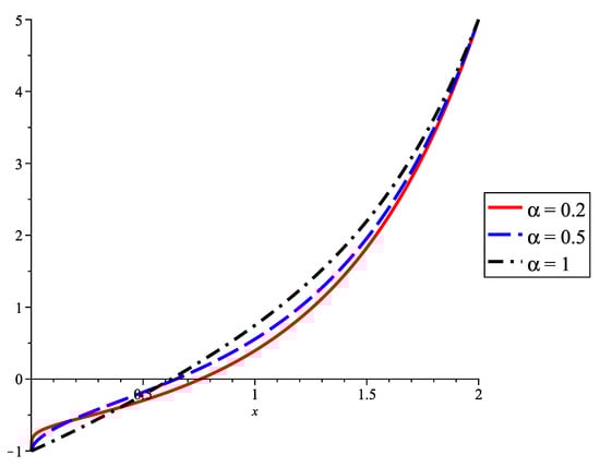
As a numerical example, if we take $b=2$, ${\delta }_1=-1,$ and ${\delta }_2=5$, the solutions to the BVP (12), (13), for $\alpha =0.2$, $\alpha =0.5$, and $\alpha =1$ are presented in Figure 1 by using red, blue, and black lines, respectively.

Figure 1. Solutions to BVP in Example 1 for different values of $\alpha$.

Example 2.

Let us consider the inhomogeneous fractional differential equation

$$\left({\widehat{D}}_{0+}^{3\alpha }y\right)\left(x\right)-x^{\alpha }\left({\widehat{D}}_{0+}^{\alpha }y\right)\left(x\right)-y\left(x\right)=1-2x^{\alpha };x\in [0,b],\alpha \in (0,1].$$

(22)

and the boundary value problem

$$y\left(0\right)={\delta }_1,\left({\widehat{D}}_{0+}^{\alpha }y\right)\left(0\right)={\delta }_2,y\left(b\right)={\delta }_3,$$

(23)

where ${\delta }_1,{\delta }_2,$ and ${\delta }_3$ are arbitrary real numbers.

As in Example 1, let us assume that the function $y=y\left(x\right)$ of the form (14) is a solution to the fractional differential Equation (22). Then, for $n\ge 1$, we find

$$a_{n+3}=\frac{\Gamma (n\alpha +1)}{\Gamma \left(\right(n+3)\alpha +1)}\left(a_n\left(\frac{\Gamma (n\alpha +1)}{\Gamma \left(\right(n-1)\alpha +1)}+1\right)+c_n\right)$$

(24)

and $a_3=\frac{a_0+c_0}{\Gamma (3\alpha +1)}$, where $c_0=1,c_1=-2$, and $c_n=0$, for all $n\ge 2$.

Let $\tilde{y}$ be a solution to the fractional differential Equation (22) satisfying the initial conditions

$$\tilde{y}\left(0\right)={\delta }_1,\left({\widehat{D}}_{0+}^{\alpha }\tilde{y}\right)\left(0\right)={\delta }_2,\left({\widehat{D}}_{0+}^{2\alpha }\tilde{y}\right)\left(0\right)=s,$$

(25)

where s is a real parameter. Then, by Theorem 3, the initial value problem (22), (25) has a unique solution $\tilde{y}(x,s)$, given by (18), where the coefficients ${\tilde{a}}_n$ satisfy (24) and ${\tilde{a}}_0={\delta }_1$, ${\tilde{a}}_1=\frac{{\delta }_2}{\Gamma (\alpha +1)}$, ${\tilde{a}}_2=\frac{s}{\Gamma (2\alpha +1)}$, and ${\tilde{a}}_3=\frac{{\delta }_1+c_0}{\Gamma (3\alpha +1)}$. Hence, for $k\ge 1$, we find

$${\tilde{a}}_{3k}=\frac{{\delta }_1+c_0}{\Gamma (3k\alpha +1)}\prod _{j=1}^{k-1}\left(\frac{\Gamma (3j\alpha +1)}{\Gamma \left(\right(3j-1)\alpha +1)}+1\right),$$

$${\tilde{a}}_{3k+1}=\frac{\Gamma (\alpha +1)({\delta }_2(1+\frac{1}{\Gamma (\alpha +1)})+c_1)}{\Gamma \left(\right(3k+1)\alpha +1)}\prod _{j=1}^{k-1}\left(\frac{\Gamma \left(\right(3j+1)\alpha +1)}{\Gamma (3j\alpha +1)}+1\right)$$

and

$${\tilde{a}}_{3k+2}=\frac{s}{\Gamma \left(\right(3k+2)\alpha +1)}\prod _{j=0}^{k-1}\left(\frac{\Gamma \left(\right(3j+2)\alpha +1)}{\Gamma \left(\right(3j+1)\alpha +1)}+1\right).$$

(26)

Thus, we notice that only the coefficients of the form ${\tilde{a}}_{3k+2}$ depend on s. We denote ${\tilde{a}}_{3k+2}=s{d}_{3k+2}$ and ${\tilde{a}}_{3k}=d_{3k}$, ${\tilde{a}}_{3k+1}=d_{3k+1}$, for every $k=0,1,\dots$ and

$$g\left(x\right)=\sum _{k=0}^{\infty }{d}_{3k}{x}^{3k\alpha }+\sum _{k=0}^{\infty }{d}_{3k+1}{x}^{(3k+1)\alpha },h\left(x\right)=\sum _{k=0}^{\infty }{d}_{3k+2}{x}^{(3k+2)\alpha }.$$

The series above have the radius of convergence ∞, so they are absolutely convergent $[0,b]$ and we have

$$\tilde{y}(x,s)=g\left(x\right)+sh\left(x\right).$$

(27)

To obtain a solution to the boundary value problem (22), (23) we have to find s such that

$$\tilde{y}(b,s)=g\left(b\right)+sh\left(b\right)={\delta }_3,$$

so

$$s=\frac{{\delta }_3-f\left(b\right)}{g\left(b\right)}.$$

The uniqueness of the solution follows as in Example 1.

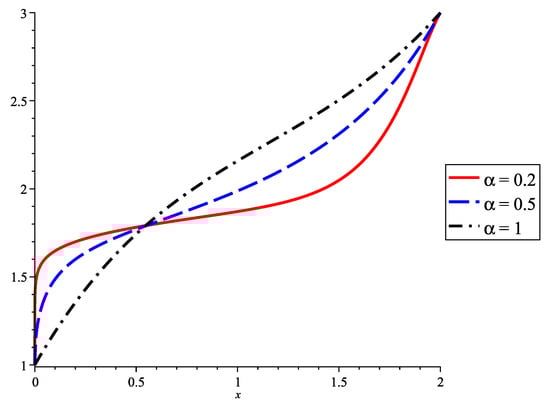
As a numerical example, we take $b=2$, ${\delta }_1=1,$${\delta }_2=2$, and ${\delta }_3=3$. The solutions to the BVP (22), (23), for $\alpha =0.2$, $\alpha =0.5$, and $\alpha =1$ are presented in Figure 2, by using red, blue, and black lines, respectively.

Figure 2. Solutions to BVP in Example 2 for different values of $\alpha$.

4. Fractional Analytic Functions

A function is said to be representable as an $\alpha$-fractional power series at $x_0$ if it is equal to the sum of the fractional Taylor series about $x_0$ on an interval $[x_0,x_0+r)$. Some authors (see [2], Definition 7.8) call such functions α-analytic at $x_0$. In the following, we define the $\alpha$-analytic functions on an open interval.

Definition 4.

Let I be an open interval and $\alpha \in (0,1]$. A real function f defined on I is called α-analytic on I, if, for every $x_0\in I$, there exists $\epsilon >0$ such that $J_{x_0,\epsilon }=[x_0,x_0+\epsilon )\subset I$ and f can be represented as an α-fractional power series at $x_0$, $f\left(x\right)={\displaystyle \sum _{n=0}^{\infty }}{a}_n{(x-x_0)}^{n\alpha }$, for all $x\in J_{x_0,\epsilon }$.

Remark 2.

By Definition 4, it follows that f is an α-fractional analytic on I, if, for every $x_0\in I$, there exists $\epsilon >0$ such that ${\overline{J}}_{x_0,\epsilon }=(x_0-\epsilon ,x_0+\epsilon )\subset I$ and the real function ${\mathit{S}}_{x_0,\epsilon }\left(f\right)$ defined by

$${\mathit{S}}_{x_0,\epsilon }\left(f\right)\left(x\right)=\left\{\begin{array}{cc}f\left(x\right)& \mathrm{if}x\in [x_0,x_0+\epsilon )\\ f(2x_0-x)& \mathrm{if}x\in (x_0-\epsilon ,x_0),\end{array}\right.$$

can be represented as an α-fractional power moduli series (2) at $x_0$ on ${\overline{J}}_{x_0,\epsilon }$.

If $\alpha =1$ in Definition 4, then the classical real analytic functions are obtained. A well-known result (see [27], Corollary 1.2.4) establishes that the sum of a power series, $f\left(x\right)={\displaystyle \sum _{n\ge 0}}{a}_n{(x-x_0)}^n$, is analytic on the interval $(x_0-r,x_0+r)$, where r is the radius of convergence of the series. In the following, we discuss the analyticity of the functions representable as fractional power series.

Let $f\left(x\right)={\displaystyle \sum _{n\ge 0}}{a}_n{(x-x_0)}^{n\alpha }$, for all $x\in (x_0,x_0+r),$$\alpha \in (0,1)$ be a function representable as an $\alpha$-fractional power series at $x_0$. Then, f can be written as $f=g\circ h$, where $g:(-r^{\alpha },r^{\alpha })\to \mathbb{R}$, $g\left(y\right)={\displaystyle \sum _{n\ge 0}}{a}_n{y}^n$, and $h:(x_0,x_0+r)\to \mathbb{R}$, $h\left(x\right)={(x-x_0)}^{\alpha }$. By the remark above, g is an analytic function. Since, for any $x_1\in (x_0,x_0+r)$, $h\left(x\right)$ can be written as $h\left(x\right)={\displaystyle \sum _{n\ge 0}}{(-1)}^n\alpha (\alpha -1)\dots (\alpha -n+1){(x_1-x_0)}^{\alpha -n}{\left(x-x_1\right)}^n$ in a small neighbourhood of $x_1$, it follows that $h\left(x\right)$ is also analytic on $(x_0,x_0+r)$, so the composite function $f=g\circ h$ is also an analytic function (see [27], Proposition 1.4.2).

Theorem 4

([6]). If $f\left(x\right)$ can be represented as an α-fractional power series at $x_0$,

$$f\left(x\right)=\sum _{n\ge 0}{a}_n{(x-x_0)}^{n\alpha },forallx\in [x_0,x_0+r),$$

(28)

where $\alpha \in (0,1]$ and $r>0$, then f is a real analytic function on the interval $(x_0,x_0+r)$.

Obviously, an (integer) power series can be also considered as an $\alpha$-fractional power series, for any $\alpha =\frac{1}{m}$, $m\in {\mathbb{N}}^{*}$. Hence, any real analytic function on an open interval I is also an $\alpha$-analytic function on I (with $\alpha =\frac{1}{m}$). By Theorem 4, it follows that any $\alpha$-analytic function on I is real analytic on I and, from Remark 1, we obtain that $\alpha$ must be a rational number if f is non-constant. On the other hand, if $\alpha =\frac{k}{m}$ with $k>1$, then, for any $x_0\in I$, we have $f\left(x\right)={\displaystyle \sum _{n=0}^{\infty }}\frac{f^{\left(kn\right)}\left(x_0\right)}{\left(kn\right)!}{(x-x_0)}^{kn}$ in a neighbourhood of $x_0$, so $f^{\prime }\left(x_0\right)=0$ for all $x_0\in I$ and the next corollary follows.

Corollary 3.

Let I be an open interval and $f:I\to \mathbb{R}$ be a non-constant function. Then, f is an α-analytic function if and only if $\alpha =\frac{1}{m}$, $m\in {\mathbb{N}}^{*}$, and f is real analytic on I.

5. Conclusions

In this paper, we study the properties of the $\alpha$-fractional power moduli series as a generalization of the $\alpha$-fractional power series. Using the generalized Taylor’s formula with fractional derivatives, a sufficient condition for a function to be represented as an $\alpha$-fractional power moduli series is established.

Moreover, we present a practical method to solve the boundary value problems for fractional differential equations, the solution being expressed as an $\alpha$-fractional power series.

Finally, $\alpha$-analytic functions are defined and we prove that a non-constant function is $\alpha$-analytic on an open interval I if and only if $\alpha =\frac{1}{m}$ with m a positive integer, and the function is real analytic on I.

References

- Diethelm, K. The Analysis of Fractional Differential Equations: An Application-Oriented Exposition Using Differential Operators of Caputo Type; Springer: Berlin, Germany, 2010. [Google Scholar]
- Kilbas, A.A.; Srivastava, H.M.; Trujillo, J.J. Theory and Applications of Fractional Differential Equations; Elsevier: Amsterdam, The Netherlands, 2006. [Google Scholar]
- Li, C.; Zeng, F. Numerical Methods for Fractional Calculus; CRC Press, Taylor & Francis Group: Boca Raton, FL, USA, 2015. [Google Scholar]
- Miller, K.S.; Ross, B. An Introduction to the Fractional Calculus and Fractional Differential Equations; John Willey & Sons: New York, NY, USA, 1993. [Google Scholar]
- Podlubny, I. Fractional Differential Equations; Academic Press: New York, NY, USA, 1999. [Google Scholar]
- El-Ajou, A.; Arqub, O.A.; Zhour, Z.A.; Momani, S. New Results on Fractional Power Series: Theories and Applications. Entropy 2013, 15, 5305–5323. [Google Scholar] [CrossRef]
- Caratelli, D.; Natalini, P.; Ricci, P.E. Examples of expansions in fractional powers, and applications. Symmetry 2023, 15, 1702. [Google Scholar] [CrossRef]
- Caratelli, D.; Natalini, P.; Ricci, P.E. Fractional differential equations and expansions in fractional powers. Symmetry 2023, 15, 1842. [Google Scholar] [CrossRef]
- Krishnasamy, V.S.; Mashayekhi, S.; Razzaghi, M. Numerical solutions of fractional differential equations by using fractional Taylor basis. IEEE/CAA J. Autom. Sin. 2017, 4, 98–106. [Google Scholar] [CrossRef]
- Syam, M.I. A numerical solution of fractional Lienard’s equation by using the residual power series method. Mathematics 2018, 6, 1. [Google Scholar] [CrossRef]
- Dimitrov, Y.; Dimov, I.; Todorov, V. Numerical Solutions of Ordinary Fractional Differential Equations with Singularities. In Advanced Computing in Industrial Mathematics. BGSIAM 2017. Studies in Computational Intelligence; Georgiev, K., Todorov, M., Georgiev, I., Eds.; Springer: Cham, Switzerland, 2019; Volume 793, pp. 77–91. [Google Scholar]
- Ren, F.; Hu, Y. The fractional power series method: An efficient candidate for solving fractional systems. Therm. Sci. 2018, 22, 1745–1751. [Google Scholar] [CrossRef]
- Angstmann, C.N.; Henry, B.I. Generalized fractional power series solutions for fractional differential equations. Appl. Math. Lett. 2020, 102, 106107. [Google Scholar] [CrossRef]
- Srivastava, H.M. An introductory overview of fractional-calculus operators based upon the Fox-Wright and related higher transcendental functions. J. Adv. Eng. Comput. 2021, 5, 135–166. [Google Scholar] [CrossRef]
- Srivastava, H.M. Some parametric and argument variations of the operators of fractional calculus and related special functions and integral transformations. J. Nonlinear Convex Anal. 2021, 22, 1501–1520. [Google Scholar]
- Rezapour, S.; Boulfoul, A.; Tellab, B.; Samei, M.E.; Etemad, S.; George, R. Fixed Point Theory and the Liouville–Caputo Integro-Differential FBVP with Multiple Nonlinear Terms. J. Funct. Spaces 2022, 2022, 6713533. [Google Scholar] [CrossRef]
- Mohammadi, H.; Baleanu, D.; Etemad, S.; Rezapour, S. Criteria for existence of solutions for a Liouville–Caputo boundary value problem via generalized Gronwall’s inequality. J. Inequal. Appl. 2021, 2021, 36. [Google Scholar] [CrossRef]
- Benchohra, M.; Hamani, S.; Ntouyas, S.K. Boundary value problems for differential equations with fractional order and nonlocal conditions. Nonlinear Anal. 2009, 71, 2391–2396. [Google Scholar] [CrossRef]
- Al-Nana, A.A.; Batiha, I.M.; Momani, S.A. Numerical approach for dealing with fractional boundary value problems. Mathematics 2023, 11, 4082. [Google Scholar] [CrossRef]
- Odibat, Z.; Shawagfeh, N. Generalized Taylor’s formula. Appl. Math. Comput. 2007, 186, 286–293. [Google Scholar] [CrossRef]
- Caputo, M. Linear models of dissipation whose Q is almost frequency independent—II. J. R. Astron. Soc. 1967, 13, 529–539. [Google Scholar] [CrossRef]
- Liouville, J. Memoire sur quelques questions de géométrie et de mécanique, et sur un nouveau genre de calcul pour résoudre ces questions. J. Ecole Polytech. 1832, 21, 1–69. [Google Scholar]
- Groza, G.; Jianu, M. Functions represented into fractional Taylor series. ITM Web Conf. 2019, 29, 010117. [Google Scholar] [CrossRef]
- Kiryakova, V. Generalized Fractional Calculus and Applications; Pitman Res. Notes in Math. Ser. 301; Longman: Harlow, UK, 1994. [Google Scholar]
- Abramowitz, M.; Stegun, I.A. Handbook of Mathematical Functions with Formulas, Graphs, and Mathematical Tables; Applied Mathematics Series; United States Department of Commerce: Washington, DC, USA; National Bureau of Standards: Washington, DC, USA; Dover Publications: New York, NY, USA, 1972; Volume 55.
- Ascher, U.M.; Mattheij, R.M.; Russell, R.D. Numerical Solutions of Boundary Value Problems for Ordinary Differential Equations; SIAM: Philadelphia, PA, USA, 1995. [Google Scholar]
- Krantz, S.G.; Parks, H.R. A Primer of Real Analytic Functions; Birkhäuser: Boston, MA, USA, 1992. [Google Scholar]
Disclaimer/Publisher’s Note: The statements, opinions and data contained in all publications are solely those of the individual author(s) and contributor(s) and not of MDPI and/or the editor(s). MDPI and/or the editor(s) disclaim responsibility for any injury to people or property resulting from any ideas, methods, instructions or products referred to in the content. |
© 2024 by the authors. Licensee MDPI, Basel, Switzerland. This article is an open access article distributed under the terms and conditions of the Creative Commons Attribution (CC BY) license (https://creativecommons.org/licenses/by/4.0/).