Consistency Improvement in the Analytic Hierarchy Process

Abstract

Consistency checking is one of the reasons for the Analytic Hierarchy Process (AHP) leadership in publications on multiple criteria decision-making (MCDM). Consistency is a measure of the quality of data input in the AHP. The theory of AHP provides indicators for the consistency of data. When an indicator is out of the desired interval, the data must be reviewed. This article presents a method for improving the consistency of reviewing the data input in an AHP application. First, a conventional literature review is presented on the theme. Then, an innovative tool of artificial intelligence is shown to confirm the main result of the conventional review: this topic is still attracting interest from AHP and MCDM researchers. Finally, a simple technique for consistency improvement is presented and illustrated with a practical case of MCDM: supplier selection by a company.

1. Introduction

The multiple criteria decision-making (MCDM) approach contributes to decision-making in situations where multiple alternatives must be evaluated considering multiple criteria [1]. The MCDM is a methodology, a collection of methods developed from the 1960s to solve decision problems [2]. This article is focused on the Analytic Hierarchy Process (AHP), a leading MCDM method for decades [3,4,5]. One main reason for the AHP’s leadership in publications on MCDM is its solid mathematical foundation [6]. The AHP’s fundamentals provide a ground for research and development of this MCDM method. The AHP theory and practice have “seven pillars”, which include the following [7]:

• Ratio scales derived from reciprocal pairwise comparisons.
• Pairwise comparisons and the 1–9 Saaty Scale.
• Sensitivity of the eigenvector to judgments.
• Extending the scale from 1 to 9 to 1–$\mathbb{R}$.
• Additive synthesis of priorities.
• Rank preservation or rank reversal.
• Group decision-making with an aggregation of individual judgments or priorities.

Another main reason for the great number of AHP publications is the need to solve practical problems with a handy tool. AHP applications include the following [6,8]:

• Educational decisions: Admitting students and faculty selection.
• Financial and marketing decisions: Advertising, credit analysis, downsizing, project management, and resource allocation.
• Governmental or social decisions: Affirmative action, energy and fuel regulations, food and drug, and smoking policies.
• Human resources and personal decisions: Career choices, entrepreneurial development, performance evaluations, and human tracking.
• Sports decisions: Drafts, predictions, and salary cap.
• Supply chain decisions: Information technology, logistics, outsourcing, and supplier and vendor selection.

The pairwise comparison matrix A of a set of n objects is a central element in the AHP. Components of $\mathit{A}=\left[a_{ij}\right]$ represent $w_i/w_j$ [9], where w is the vector of the weights for the compared objects $i=1,2,3\dots n$. Equation (1) presents one way to generate w from A:

$$\mathit{A}\mathit{w}={\lambda }_{\max }\mathit{w}$$

(1)

where w is the right eigenvector of A, and ${\lambda }_{\max }$ is its maximum eigenvalue.

To be consistent means no change of mind. Consistency is “conformity with previous practice” [8]. A 100%-consistent pairwise comparison matrix A satisfies Equation (2):

$$a_{ij}=w_i/w_j$$

(2)

$\forall i,j=1,2,3\dots n$.

A consequence of the consistency of A is presented in Equation (3) [10]:

$$\begin{array}{c}\hfill a_{ij}=\frac{w_i}{w_j}=\frac{w_i/w_k}{w_j/w_k}=\frac{a_{ik}}{a_{jk}}\end{array}$$

$$\begin{array}{c}\hfill a_{ik}=a_{ij}{a}_{jk}\end{array}$$

(3)

$\forall i,j,k=1,2,3\dots n$.

In the AHP, pairwise comparisons are usually performed regarding a linear 1–9 scale, which is named the Saaty Scale here but is also named “The Scale” [11] or “Fundamental Scale of Absolute Numbers” [8]. With the Saaty Scale, A becomes a positive reciprocal matrix, satisfying conditions $a_{ij}>0$ and $a_{ij}=1/a_{ji}$, $\forall i,j=1,2,3\dots n$. A consequence of this positiveness and reciprocity is that ${\lambda }_{\max }\ge n$. A corollary from consistency is ${\lambda }_{\max }=n$ [11].

Despite some criticism and the proposal of different scales [12,13], the Saaty Scale prevails in AHP applications [14]. After all, the Saaty Scale allows for comparisons concerning weight dispersion and weight uncertainty [15]. Nevertheless, the use of the Saaty Scale does not guarantee that A will be a consistent matrix, satisfying Equations (2) and (3). In the example below, A, B, and C are all pairwise comparison matrices obtained with the Saaty Scale. However, only A is 100% consistent; B and C are not:

$$\begin{array}{c}\hfill \mathit{A}=\left[\begin{array}{ccc}1& 3& 9\\ 1/3& 1& 3\\ 1/9& 1/3& 1\end{array}\right],\mathit{B}=\left[\begin{array}{ccc}1& 3& 5\\ 1/3& 1& 3\\ 1/5& 1/3& 1\end{array}\right],\mathit{C}=\left[\begin{array}{ccc}1& 7& 3\\ 1/7& 1& 3\\ 1/3& 1/3& 1\end{array}\right]\end{array}$$

The consistency of A is noted with $a_{12}{a}_{23}$ = 3 × 3 = 9 = $a_{13}$. The inconsistency of B and C is noted with $b_{12}{b}_{23}$ = 3 × 3 ≠ 5 = $b_{13}$ and $c_{12}{c}_{23}$ = 7 × 3 ≠ 3 = $c_{13}$. The eigenvalues for A, B, and C are ${\lambda }_{{\max }_A}$ = 3, ${\lambda }_{{\max }_B}$ ≈ 3.04, and ${\lambda }_{{\max }_C}$ ≈ 3.99, respectively. The eigenvectors are ${\mathit{w}}_A\approx [0.69,0.23,0.08]$, ${\mathit{w}}_B\approx [0.64,0.26,0.10]$, and ${\mathit{w}}_C\approx [0.69,0.19,0.12]$. As A is 100% consistent, one question arises: By how much are B and C inconsistent matrices? Since ${\lambda }_{{\max }_B}$ and $w_B$ are closer to ${\lambda }_{{\max }_A}$ and $w_A$ than ${\lambda }_{{\max }_C}$ and $w_C$, it seems that B is less inconsistent than C. Therefore, Q1 and Q2 are two research questions:

Q1:

How can we measure the consistency of a pairwise comparison matrix?

Q2:

How can we improve the consistency of a pairwise comparison matrix?

To answer Q1 and Q2, this article presents a literature review on consistency measurement and consistency improvement (Section 2), with innovative support from artificial intelligence (AI) in Section 2.2. Then, a simple technique for consistency improvement is presented (Section 3) with a practical case of MCDM: a supplier selection by a manufacturing company (Section 4). Finally, Section 5 presents this article’s conclusions and proposal for future research.

2. Literature Review

2.1. Background

Consistency and the Saaty Scale have been major subjects in AHP theory since the presentation of the seminal works [11,16,17]. The first document published on the AHP [16] introduced the Saaty Scale, with the former name “The Scale” but starting with zero being defined for “not comparable” when “there is no meaning to compare two objects”. The document does not address the consistency measurement, focusing on obtaining the weights with the eigenvector.

The subsequent documents published on the AHP [11,18,19,20,21,22] updated the Saaty Scale, deleting the zero, as presented in Table 1:

Table 1. Saaty Scale [8,11,17,18,19,20,21,22].

Intensity of Importance	Definition	Explanation
1 1	Equal importance	The two compared objectives have the same importance
3	Moderate importance	Experience and judgment slightly favor one object over another
5	Strong importance	Experience and judgment strongly favor one object over another
7	Demonstrated importance	One object is very strongly favored and this dominance is demonstrated in practice
9	Absolute importance	The evidence favoring one object over another is of the highest possible order of affirmation
Reciprocals of above		If object i has one of the above nonzero numbers when compared to j, then j has the reciprocal value when compared to i
Rationals	Ratios arising from the scale	If consistency were to be forced or when measurements are available

¹ In two-object problems, one may use $1+ϵ,0<ϵ\le 1/2$, to indicate very slight dominance between two nearly equal objects.

Documents published previously, other than the AHP’s eponymous book (Saaty, 1980) [17], average 65.3 citations, as presented in Table 2. The outlier is Saaty (1977) [11] with over 6000 citations, the most cited document on MCDM [6].

Table 2. Citations of the first published documents on the AHP.

Authorship (Year) [Reference]	Title of the Document	Citations
Saaty (1974) [16]	Measuring the fuzziness of sets	100
Saaty and Khouja (1976) [18]	A measure of world influence	41
Saaty and Rodgers (1976) [19]	Higher education in the United States (1985–2000). Scenario construction using a hierarchical framework with eigenvector weighting	76
Alexander and Saaty (1977) [20]	The forward and backward processes of conflict analysis	45
Saaty (1977) [11]	A scaling method for priorities in hierarchical structures	6636
Saaty (1977) [21]	Scenarios and priorities in transport planning: Application to Sudan	58
Saaty and Bennett (1977) [22]	A theory of analytical hierarchies applied to political candidacy	72

Source: www.scopus.com (accessed on 6 December 2023).

Saaty (1977) [11] introduced the consistency measurement, proposing the consistency index CI as in Equation (4):

$$CI=\frac{{\lambda }_{\max }-n}{n-1}$$

(4)

If A is 100% consistent, then ${\lambda }_{\max }=n$ and $CI=0$. In this case, Equations (2) and (3) are satisfied.

The consistency ratio CR is a better measure for the consistency of a comparison matrix since it compares CI with a random index RI obtained with the simulation of positive reciprocal matrices [23,24,25], as presented in Equation (5):

$$CR=\frac{CI}{RI}$$

(5)

Table 3 presents values for $RI$ as a function of the matrix order n.

Table 3. Random consistency indexes.

n	Original	ORNL–PITT (1982)	EC–GWU (1990)	UU (1991)	Usual
3	0.416	0.58	0.52333	0.4887	0.52
4	0.851	0.90	0.88604	0.8045	0.89
5	1.115	1.12	1.10983	1.0591	1.11
6	1.150	1.24	1.25390	1.1797	1.25
7	1.345	1.32	1.34516	1.2519	1.35
8	1.334	1.41		1.3171	1.40
9	1.315	1.45		1.3733	1.45
10	1.420	1.49		1.4055	1.49
11	1.395	1.51		1.4213	1.51
12	1.482	1.48		1.4497	1.54
13	1.491	1.56		1.4643	1.56
14	1.470	1.57		1.4822	1.57
15	1.466	1.59		1.4969	1.58

In the AHP literature, $RI$ values vary because they were obtained with different numbers of randomly simulated matrices. Originally, RI was obtained with 50 matrices for each n [11]. A study performed at the University of Pittsburgh (PITT) with support from the Oak Ridge National Laboratory (ORNL) increased the number of matrices to 500 [26]. A statistical experiment conducted at the George Washington University (GWU) with the Software Expert Choice (EC) experimented with incomplete matrices [27], increasing the number of simulated matrices to thousands. Perhaps the most accurate estimation for RI was performed in the University of Ulster (UU), Northern Ireland [28]. However, the usual values for RI are presented in the last column of Table 3. The usual values combine the ORNL–PITT values with EC–GWU: for $n\le 7$, the usual values are the EC-CWU values rounded to hundredths; for $n>7$, the usual values are the same for ORNL–PITT [8].

Table 4 presents values of $CR$ for matrices A, B, and C (Section 1) for $RI$ presented in Table 3.

Table 4. Consistency ratio values with different random consistency indexes.

Matrix	Original	ORNL–PITT	EC–GWU	UU	Usual
A	0	0	0	0	0
B	0.05	0.03	0.04	0.04	0.04
C	1.62	1.16	1.28	1.37	1.29

As ${\lambda }_{{\max }_A}$ = 3, then $C{I}_A$ = 0, resulting in $C{R}_A$ = 0 for all $RI$ values. This result is expected since A is a 100%-consistent matrix, satisfying Equations (2) and (3).

As ${\lambda }_{{\max }_B}\approx 3.04$, then $C{I}_B\approx 0.02$, making $C{R}_B$ vary from 0.03 to 0.04. As ${\lambda }_{{\max }_C}\approx 3.99$, then $C{I}_C\approx 0.22$, making $C{R}_C$ vary from 0.38 to 0.53. $C{R}_B$ and $C{R}_C$ are expected to be greater than zero, since B and C are not 100%-consistent matrices. However, $C{R}_C>C{R}_B$, indicating that C is more inconsistent than B. The question is as follows: is the inconsistency of B or C acceptable? To answer this question, the 0.1 threshold was proposed [11].

The 0.1 threshold considers that the normalized values for $w_i$ are from 0 to 1; the required order for $RI$ was as small as 10% but not smaller than 1% because inconsistency itself is important, since “without it new knowledge that changes preferences cannot be admitted” [9]. Saaty [17] further suggested that for matrices of orders three and four, the thresholds could be 0.5 and 0.8, respectively [29]. For larger matrices, even a CR = 0.2 could be tolerated, but no more [30]. Other consistency indices were proposed, such as the geometrical consistency index [31]. In this article, the usual $CI$, $CR$, and its 0.1 threshold are adopted. This adoption is for an alignment with the original AHP theory and its usual practice.

Considering the 0.1 threshold, B is not 100% consistent, but it is an acceptable matrix, and C is an inconsistent unacceptable matrix. Then, the $c_{ij}$ components of C must be revised to improve its consistency, or simply to increase $C{R}_C$.

One simple way to increase the $CR$ of a comparison matrix is by comparing the differences between its components and the components of a 100%-consistent matrix. As the components with greater differences are more inconsistent with the others, these components are first suggested to be revised. The differences compose the deviations matrix $\overline{\mathit{C}}$ as in Equation (6):

$${\overline{c}}_{ij}=|c_{ij}-w_{C_i}/w_{C_j}|$$

(6)

$\forall i,j=1,2,3\dots n.$

In our case, $\overline{\mathit{C}}$ is as follows:

$$\begin{array}{c}\hfill \overline{\mathit{C}}=\left[\begin{array}{ccc}0& 3.34& 2.74\\ 0.13& 0& 1.43\\ 0.16& 0.30& 0\end{array}\right]\end{array}$$

As $c_{12}=3.34$ is the greatest component of $\overline{\mathit{C}}$, it is suggested that it should be revised from $c_{12}=7$ to $c_{12}^{\prime }=w_1/w_2\approx 0.69/0.19\approx 3.66$, resulting in $C^{\prime }$:

$$\begin{array}{c}\hfill {\mathit{C}}^{\prime }=\left[\begin{array}{ccc}1& 3.66& 3\\ 0.27& 1& 3\\ 1/3& 1/3& 1\end{array}\right]\end{array}$$

${\lambda }_{{max}_{{\mathit{C}}^{\prime }}}\approx 3.64$ and $C{R}_{{\mathit{C}}^{\prime }}\approx 0.17$. C′ is less inconsistent than C, but the inconsistency of both matrices is unacceptable since $C{R}_C$ and $C{R}_{C^{\prime }}$ are greater than the 0.1 threshold.

With one more iteration, ${\mathit{C}}^{\prime \prime }$ is found:

$$\begin{array}{c}\hfill {\mathit{C}}^{\prime \prime }=\left[\begin{array}{ccc}1& 2.66& 3\\ 0.38& 1& 3\\ 1/3& 1/3& 1\end{array}\right]\end{array}$$

${\lambda }_{{max}_{{\mathit{C}}^{\prime \prime }}}\approx 3.04$ and $C{R}_{{\mathit{C}}^{\prime \prime }}\approx 0.04$. Now, C″ is an acceptable pairwise comparison matrix with $C{R}_{C^{\prime \prime }}\approx 0.096$. The changes from C to C″ result in $w_C^{\prime \prime }\approx [0.58,0.27,0.16]$, different than the former $w_c$. Of course, this would need approval by the decision-maker or by whoever is in charge of making the comparisons.

The simple A–B–C example illustrates the concepts and variables of consistency as CI and CR. Section 3 presents a technique for consistency improvement in more complex cases with $n>3$. Before it, the next subsection presents how consistency has been measured and analyzed in the more recent AHP literature.

2.2. Recent Literature on Consistency Measurement and Improvement

The literature on consistency measurement of pairwise comparison matrix is a major part of the AHP literature. Therefore, it has also been prolific in the literature since the 1970s. This section focuses on the last ten years: documents published from 2013. This is the focus of the new Scopus Database tool, its artificial intelligence (AI) tool.

Most literature reviews are based on two databases: Clarivate’s Web of Science or Elsevier’s Scopus [32]. Despite both databases having similar contents, Scopus was selected for this research because it is free through institutional access [5]. Despite expected similar contents between Scopus and Web of Science, a second reason to exclusively search Scopus was the uniformity of search characteristics, such as search strings. Finally, the third reason for choosing Scopus was its new AI tool (https://www.elsevier.com/products/scopus/scopus-ai, accessed on 6 December 2023). Still in a beta phase, this tool allows for focusing on publications from recent years.

The question of “How to measure the consistency for a pairwise comparison matrix?” in the Scopus AI tool resulted in four key insights from the abstracts:

• Inconsistency reduction: Various iterative and non-iterative algorithms have been developed to reduce inconsistency in pairwise comparison matrices [33].
• Inconsistency indices: Different inconsistency indices have been proposed to measure the deviation from a consistent matrix, such as Koczkodaj’s inconsistency index, Saaty’s inconsistency index, geometric inconsistency index, and logarithmic Manhattan distance [34,35,36].
• New measures: Some studies have introduced new inconsistency measures for incomplete pairwise comparison matrices and interval pairwise comparison matrices [36,37].
• Comparative analysis: Comparative analyses have been conducted to evaluate the performance of different inconsistency indices using Monte Carlo simulations [33,37].

Scopus AI concludes that “there are several methods and indices available to measure the consistency of pairwise comparison matrices, and their effectiveness can be evaluated through comparative analyses and simulations” (https://www.scopus.com/search/form.uri?display=basic#scopus-ai, accessed on 29 December 2023).

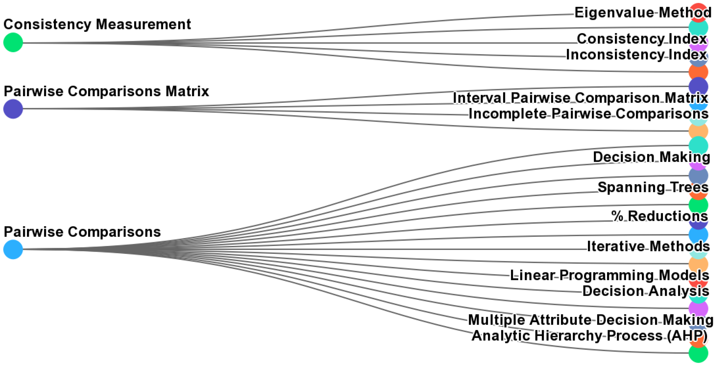
Figure 1 presents a “conceptual map” generated by Scopus AI. This map groups the keywords into three branches, separating pairwise comparisons from the pairwise comparison matrix.

Figure 1. Conceptual map for “How to measure the consistency for a pairwise comparison matrix?”. Source: Scopus AI.

Scopus AI concludes by highlighting three topics for expert research:

• What are the mathematical methods used to measure consistency in pairwise comparison matrices?
• How does the CR help in evaluating the reliability of a pairwise comparison matrix?
• Can inconsistency in a pairwise comparison matrix affect the accuracy of decision-making processes?

These three points are connected, indeed. For instance, if the CR helps in evaluating the reliability of a pairwise comparison matrix, it affects the accuracy of the decision-making process.

The literature review concludes that CR and the 0.1 threshold have been accepted for the consistency measurements and analyses of pairwise comparison matrices.

3. Consistency Improvement

Section 1 and Section 2.1 present the A–B–C example with three 3-n pairwise comparison matrices. Real problems certainly involve more matrices with $n>3$. Therefore, consistency improvement becomes more complex.

With $n=2$, there is no possibility for inconsistency, since $k=i$ or $k=j$, always satisfying Equation (3), $\forall i,j,k=1,2$. With $n=3$, and, for instance, $i=1$, $j=2$, and $k=3$, Equation (3) may not be satisfied, as it occurrs with $b_{13}\ne b_{12}{b}_{23}$ and $c_{13}\ne c_{12}{c}_{23}$. With $n\ge 4$, the possibility for inconsistency increases with three combinations of $n(n-1)/2$ comparisons.

Iterations with just one change in an inconsistent comparison matrix may not be effective. On the other hand, replacing all comparisons seems to be unfair or illogical. Therefore, we propose to change only the $a_{ij}$ comparisons, which brings significant deviation to $a_{ik}{a}_{kj}$, initially computing the expected value ${\gamma }_{ij}$ as in Equation (7):

$${\gamma }_{ij}=\frac{{\sum }_{k=1}^n{a}_{ik}{a}_{jk}}{n-2}$$

(7)

$\forall i,j,k=1,2,3\dots n$ and $j>i$.

The absolute deviation between the value provided in the comparison matrix and the expected value for consistency satisfying Equation (3) is ${\psi }_{ij}=|a_{ij}-{\gamma }_{ij}|$. For inconsistent comparison matrices, we suggest that the $a_{ij}$ with ${\psi }_{ij}$ between the average $\overline{\psi }$ plus or less one-third of its standard deviation must be replaced by $w_i/w_j$.

For instance, let us consider the 4-n pairwise comparison matrix D:

$$\begin{array}{c}\hfill \mathit{D}=\left[\begin{array}{cccc}1& 1/2& 1/3& 9\\ 2& 1& 8& 3\\ 3& 1/8& 1& 2\\ 1/9& 1/3& 1/2& 1\end{array}\right]\end{array}$$

${\lambda }_{{\max }_D}\approx 5.28$ and $C{R}_D\approx 0.43$. As $C{R}_D>0.1$, D is an inconsistent pairwise comparisons matrix, and its inconsistency is unacceptable. For D, ${\psi }_{12}\approx 1.02$, ${\psi }_{13}\approx 3.92$, ${\psi }_{14}\approx 7.92$, ${\psi }_{23}\approx 6.92$, ${\psi }_{24}=14$, and ${\psi }_{34}\approx 11.69$. The average value is $\overline{\psi }\approx 7.58$, and its standard deviation is approximately 4.80. Only ${\psi }_{14}$ and ${\psi }_{23}$ are in the interval [5.98, 9, 18]. Then, D′ is obtained by replacing $d_{14}$ and $d_{23}$ by ${\gamma }_{14}$ and ${\gamma }_{23}$, respectively:

$$\begin{array}{c}\hfill {\mathit{D}}^{\prime }=\left[\begin{array}{cccc}1& 1/2& 1/3& 1\\ 2& 1& 1& 3\\ 3& 1& 1& 2\\ 1& 1/3& 1/2& 1\end{array}\right]\end{array}$$

${\lambda }_{{\max }_{D^{\prime }}}\approx 4.40$ and $C{R}_{D^{\prime }}\approx 0.016$. As $C{R}_{D^{\prime }}<0.1$, D′ is also an inconsistent pairwise comparison matrix, but its inconsistency is acceptable. However, the eigenvector also changes from $w_D=[0.22,0.52,0.18,0.07]$ to $w_{D^{\prime }}=[0.14,0.36,0.36,014]$ to be validated by the decision-maker.

It is important to note that our proposed technique for consistency improvement resulted in individual significant changes in the comparison matrix D to D′. Therefore, replacing $d_{14}$ = 9 and $d_{23}$ = 8 by $d_{14}^{\prime }$ = $d_{23}^{\prime }$ = 1 are big changes that result in a new vector of weights. These must all be validated by the decision-maker. Furthermore, this is a major limitation of our proposal. If the decision maker does not agree with the changes, then he (she or they) must review the comparisons by himself (herself or themselves). However, our proposal is not solely based on mathematics. The comparisons are connected, and the mathematics may capture the connection as presented in the next section, with a case of consistency improvement from the real world.

4. A Case of Consistency Improvement in Supply Chain Decision-Making

Supplier selection is one of the decision-making problems mostly solved by AHP applications [4]. This problem consists of choosing a single alternative (supplier) from a set of alternatives (suppliers). Table 5 presents an example of data for supplier selection considering three criteria (Delivery, Price, and Quality) and four alternatives (Suppliers 1, 2, 3, and 4):

Table 5. Example of data for a supplier selection problem.

Supplier	Delivery	Price [USD]	Quality
1	Slow	200,000	Acceptable
2	Regular	400,000	Excellent
3	Quick	300,000	Good
4	Regular	300,000	Very Good

In this case, it is clear that Quality is the most important criterion, but it is not clear by how much it is more important than others. Furthermore, it is not clear which one is more important: Delivery or Price. Then, a pairwise comparison matrix is a good tool to figure out the relative importance of the criteria. Table 6 presents a comparison matrix among the criteria.

Table 6. Pairwise comparison of the criteria for a supplier selection problem.

Criterion	Delivery	Price	Quality
Delivery	1	1/3	1/5
Price	3	1	1/3
Quality	5	3	1

The comparison matrix of the criteria has the same components of matrix B presented in Section 1. This matrix is equal to ${\mathit{B}}^T$. Then, both matrices have the same ${\lambda }_{\max }\approx 3.04$ and $CR\approx 0.04$. Therefore, this matrix is inconsistent but acceptable, since its $CR<0.1$. The decision-maker who provided the comparison matrix of the criteria understood the concepts of the Saaty Scale.

The eigenvector for the comparison matrix of the criteria has the same components of ${\mathit{w}}_B$, but in reverse order: [0.10, 0.26, 0.64]. It results in Quality being the most important criterion with 64% of weight, followed by Price and Delivery with 26% and 10%, respectively.

Table 7 presents a comparison matrix among Suppliers 1 to 4 regarding criterion Delivery. According to Table 5, Supplier 3 has the best performance in delivering quickly; Suppliers 2 and 4 deliver regularly, and Supplier 3 delivers slowly.

Table 7. Pairwise comparison of suppliers regarding their deliveries.

	Supplier 1	Supplier 2	Supplier 3	Supplier 4
Supplier 1	1	1/3	1/5	1/3
Supplier 2	3	1	1/3	1
Supplier 3	5	3	1	3
Supplier 4	3	1	1/3	1

The comparison matrix of suppliers on their deliveries has ${\lambda }_{\max }$ ≈ 4.064 and $CR$ ≈ 0.024. Therefore, this matrix is inconsistent but acceptable, since its $CR<0.1$. The eigenvector for the comparison matrix is [0.08, 0.20, 0.52, 0.20]. It results in Supplier 3 being the best in Delivery with 52% of weight, followed by Suppliers 2 and 4 tied at 20%, and Supplier 1 being the worst with 8%.

For Price, there are available data as presented in Table 5. Weights for suppliers on Price are obtained by normalizing their reciprocals, as presented in Table 8.

Table 8. Weights for suppliers regarding their prices.

Supplier	Price [USD 1000]	Reciprocal	Weight
1	200	1/200	35%
2	400	1/400	18%
3	300	1/300	24%
4	300	1/300	24%

Table 9 presents a comparison matrix for suppliers regarding the Quality criterion. According to Table 5, suppliers’ performances vary greatly: from Acceptable (Supplier 1) to Excellent (Supplier 2), including Good (Supplier 3) and Very Good (Supplier 4).

Table 9. Pairwise comparisons of suppliers regarding their quality.

	Supplier 1	Supplier 2	Supplier 3	Supplier 4
Supplier 1	1	1/7	1/3	1/5
Supplier 2	7	1	5	3
Supplier 3	3	1/5	1	3
Supplier 4	5	1/3	1/3	1

The comparison matrix of suppliers on their quality Q, has ${\lambda }_{{\max }_Q}\approx 4.39$ and $C{R}_Q\approx 0.146$. Therefore, this matrix is inconsistent and unacceptable, since $C{R}_Q>0.1$. The eigenvector for the comparison matrix is [0.06, 0.58, 0.21, 0.16]. It results in Supplier 2 as the best in Quality with 58% of weight, followed by Suppliers 3, 4, and 1 with 21%, 16%, and 5%, respectively. The weights for Suppliers 1 and 2 are expected to be the lowest and the highest ones. However, there is a clear inversion between Good Supplier 3 and Very Good Supplier 4. Then, Q must be revised.

For Q, ${\psi }_{12}\approx 0.076$, ${\psi }_{13}\approx 0.057$, ${\psi }_{14}\approx 0.514$, ${\psi }_{23}\approx 3.333$, ${\psi }_{24}$ = 5.2, and ${\psi }_{34}$ = 2.4. The average value is $\overline{\psi }\approx 1.93$, and its standard deviation is approximately 2.08. Only ${\psi }_{34}$ is in the interval [1.23, 2.62]. Then, Q′ is obtained by replacing $d_{24}$ = 3 with ${\gamma }_{14}$ = 3/5 as presented in Table 10:

Table 10. Revised pairwise comparison of suppliers regarding their quality.

	Supplier 1	Supplier 2	Supplier 3	Supplier 4
Supplier 1	1	1/7	1/3	1/5
Supplier 2	7	1	5	3
Supplier 3	3	1/5	1	3/5
Supplier 4	5	1/3	5/3	1

${\lambda }_{{\max }_{Q^{\prime }}}\approx 4.08$ and $C{R}_{Q^{\prime }}\approx 0.030$. As $C{R}_{Q^{\prime }}<0.1$, Q′ is also an inconsistent pairwise comparison matrix, but its inconsistency is acceptable. The eigenvector changes from ${\mathit{w}}_Q=[0.05,0.58,0.21,0.16]$ to ${\mathit{w}}_{Q^{\prime }}=[0.06,0.57,0.14,0.23]$, which makes much more sense considering the initial data in Table 5 with more weight for Very Good Supplier 4 than for Good Supplier 3.

Table 11 presents, again, the weights for the suppliers regarding each criterion (decision matrix), and it also presents their overall weights (decision vector).

Table 11. Decision matrix and decision vector for the case of supplier selection.

	Delivery	Price	Quality
Supplier	10%	26%	64%	Overall
1	0.08	0.35	0.06	0.14
2	0.20	0.18	0.57	0.43
3	0.52	0.24	0.14	0.20
4	0.20	0.24	0.23	0.23

Keeping the comparisons of Q (Table 9) and its eigenvector in the decision matrix would result in a different decision vector: [0.14, 0.43, 0.25, 0.18]. Both decision vectors are close to each other, indicating that Supplier 2 has the highest overall performance. However, there are significant changes in the second and third-best suppliers. Therefore, the consistency improvement in this case results in a more reliable decision. Astoundingly, the decision-maker recognized that he caused slight confusion in the last comparison, comparing Supplier 3 to Supplier 4 regarding their quality. Instead of “3”, the decision-maker was thinking of “1/3”, since the quality of Supplier 4 is better than Supplier 3’s. The mathematics of the proposed technique quickly identified this comparison as most divergent among all. Then, the decision-maker agreed with the new comparison matrix (Table 11) and its eigenvector.

Complimentary procedures such as Sensitivity Analysis or Robustness Tests are not conducted in this case because they are out of the scope of this work.

5. Conclusions

Consistency measurement and improvement is still an attractive subject of research in the AHP literature. This is evidenced by the literature review presented in Section 2. After all, consistency checking is an advantage of applying AHP instead of other MCDM methods, which do not include this check. However, when the consistency test fails, the decision process stalls.

This article presents a procedure for the improvement of consistency of pairwise comparison matrices. The simple procedure considers the means and the standard deviations to a consistent matrix. Besides being simple, it is a highly efficient procedure requiring few changes in the pairwise comparison matrix.

The first proposal for future research is the test of the proposed procedure with more cases other than in supply chain management. This proposal is very reliable due to the applicability of the AHP in many fields of decision-making, from computer science and engineering to health and medical applications. Mathematical simulations of inconsistent matrices, for instance, with Monte Carlo experiments or similar algorithms of randomness, could also be interesting.

Finally, some important advances in the AHP not included in this work may be considered in future research, such as the adoption of Fuzzy Sets Theory (FST) or the study of Group Decision-Making. Much older than the AHP literature, FST gained attention earlier this century with the proposal of Fuzzy Hesitant and Fuzzy Intuitionistic Sets. The study on consistency measurements and improvements in hybrid AHP–FST, especially with the new types of fuzzy sets, has not yet been studied.

References

- Alvarez Gallo, S.; Maheut, J. Multi-criteria analysis for the evaluation of urban freight logistics solutions: A systematic literature review. Mathematics 2023, 11, 4089. [Google Scholar] [CrossRef]
- Greco, S.; Ehrgott, M.; Figueira, J.F. Multiple Criteria Decision Analysis: State of the Art Surveys, 2nd ed.; Springer: New York, NY, USA, 2016. [Google Scholar]
- Wallenius, J.; Dyer, J.S.; Fishburn, P.C.; Steuer, R.E.; Zionts, S.; Deb, K. Multiple criteria decision making, multiattribute utility theory: Recent accomplishments and what lies ahead. Manag. Sci. 2008, 54, 1336–1349. [Google Scholar] [CrossRef]
- Khan, S.A.; Chaabane, A.; Dweiri, F.T. Multi-criteria decision-making methods application in supply chain management: A systematic literature review. In Multi-Criteria Methods and Techniques Applied to Supply Chain Management; Salomon, V., Ed.; Tech Open: London, UK, 2018; pp. 3–31. [Google Scholar]
- Ruiz Bargueno, D.; Salomon, V.A.P.; Marins, F.A.S.; Palominos, P.; Marrone, L.A. State of the art review on the Analytic Hierarchy Process and urban mobility. Mathematics 2021, 9, 3179. [Google Scholar] [CrossRef]
- Petrillo, A.; Salomon, V.A.P.; Tramarico, C.L. State-of-the-art review on the Analytic Hierarchy Process with benefits, opportunities, costs, and risks. J. Risk Financ. Manag. 2023, 16, 372. [Google Scholar] [CrossRef]
- Saaty, T.L. Fundamentals of the Analytic Hierarchy Process. In The Analytic Hierarchy Process in Natural Resource and Environmental Decision Making: Managing Forest Ecosystems; Schmoldt, D.L., Kangas, J., Mendoza, G.A., Pesonen, M., Eds.; Springer: Dordrecht, The Netherlands, 2001; Volume 3, pp. 15–35. [Google Scholar] [CrossRef]
- Saaty, T.L. Theory and Applications of the Analytic Network Process: Decision Making with Benefits, Opportunities, Costs, and Risks; RWS: Pittsburgh, PA, USA, 2013. [Google Scholar]
- Saaty, T.L. Fundamentals of Decision Making and Priority Theory with the Analytic Hierarchy Process, 1st ed.; RWS: Pittsburgh, PA, USA, 1994. [Google Scholar]
- Saaty, T.L.; Vargas, L.G. Inconsistency and rank preservation. J. Math. Psychol. 1984, 28, 205–214. [Google Scholar] [CrossRef]
- Saaty, T.L. A scaling method for priorities in hierarchical structures. J. Math. Psychol. 1977, 15, 234–281. [Google Scholar] [CrossRef]
- Ma, D.; Zheng, X. 9/9-9/1 scale method of AHP. In Proceedings of the 2nd International Symposium on the AHP, Pittsburgh, PA, USA, 11–14 August 1991; Volume 1, pp. 197–202. [Google Scholar] [CrossRef]
- Salo, A.A.; Hamalainen, R.P. On the measurement of preferences in the Analytic Hierarchy Process. J. Multi-Criteria Decis. Anal. 1997, 6, 309–319. [Google Scholar] [CrossRef]
- Asadabadi, M.R.; Chang, E.; Saberi, M.; Zhou, Z. Are MCDM methods useful? A critical review of Analytic Hierarchy Process (AHP) and Analytic Network Process (ANP). Cogent Eng. 2019, 6, 1–11. [Google Scholar] [CrossRef]
- Goepel, K.D. Comparison of judgment scales of the Analytical Hierarchy Process: A new approach. Int. J. Inf. Technol. Dec. 2019, 18, 445–463. [Google Scholar] [CrossRef]
- Saaty, T.L. Measuring the fuzziness of sets. J. Cybern. 1974, 4, 53–61. [Google Scholar] [CrossRef]
- Saaty, T.L. The Analytic Hierarchy Process; McGraw-Hill: New York, NY, USA, 1980. [Google Scholar]
- Saaty, T.L.; Khouja, M. A measure of world influence. Confl. Mana. Peace 1976, 2, 31–48. [Google Scholar] [CrossRef]
- Saaty, T.L.; Rodgers, P.C. Higher education in the United States (1985–2000): Scenario construction using a hierarchical framework with eigenvector weighting. Socio Econ. Plan. Sci. 1976, 10, 251–263. [Google Scholar] [CrossRef]
- Alexander, J.M.; Saaty, T.L. The forward and backward processes of conflict analysis. Syst. Res. 1977, 22, 87–98. [Google Scholar] [CrossRef]
- Saaty, T.L. Scenarios and priorities in transport planning: Application to the Sudan. Transport. Res. 1977, 11, 343–350. [Google Scholar] [CrossRef]
- Saaty, T.L.; Bennett, J.P. A theory of analytical hierarchies applied to political candidacy. Syst. Res. 1977, 22, 237–245. [Google Scholar] [CrossRef]
- Saaty, T.L. How to make a decision: The Analytic Hierarchy Process. Eur. J. Oper. Res. 1991, 48, 9–26. [Google Scholar] [CrossRef]
- Wedley, W.C. Consistency prediction for incomplete AHP matrices. Math. Comput. Model. 1993, 17, 151–161. [Google Scholar] [CrossRef]
- Saaty, T.L. Mathematical Principles of Decision Making, Kindle Edition; RWS: Pittsburgh, PA, USA, 2013. [Google Scholar]
- Saaty, T.L.; Vargas, L.G. The Logic of Priorities, 1st ed.; Kluwer: Boston, MA, USA, 1982. [Google Scholar]
- Forman, E.H. Random indices for incomplete pairwise matrices. Eur. J. Oper. Res. 1990, 48, 153–155. [Google Scholar] [CrossRef]
- Donegan, H.A.; Dodd, F.J. A note on Saaty’s random indexes. Math. Comput. Model. 1991, 15, 135–137. [Google Scholar] [CrossRef]
- Pant, S.; Kumar, A.; Ram, M.; Klochkov, Y.; Sharma, H.K. Consistency indices in Analytic Hierarchy Process: A review. Mathematics 2022, 10, 1206. [Google Scholar] [CrossRef]
- Saaty, T.L. Decision Making with Dependence and Feedback: The Analytic Network Process, 2nd ed.; RWS: Pittsburgh, PA, USA, 2001. [Google Scholar]
- Aguaron, J.; Moreno-Jimenez, J. The geometric consistency index: Approximated threshold. Eur. J. Oper. Res. 2003, 147, 137–145. [Google Scholar] [CrossRef]
- Mongeon, P.; Paul-Hus, A. The journal coverage of Web of Science and Scopus: A comparative analysis. Scientometrics 2016, 106, 213–228. [Google Scholar] [CrossRef]
- Mazurek, J. Inconsistency reduction. In Advances in Pairwise Comparisons. Multiple Criteria Decision Making; Springer: Cham, Switzerland, 2023. [Google Scholar] [CrossRef]
- Brunelli, M. Recent advances on inconsistency indices for pairwise comparisons—A commentary. Fund. Inform. 2016, 144, 321–332. [Google Scholar] [CrossRef]
- Csato, L.; Ágoston, K.C.; Bozoki, S. On the coincidence of optimal completions for small pairwise comparison matrices with missing entries. Ann. Oper. Res. 2023. [Google Scholar] [CrossRef]
- Dong, Y.; Chen, X.; Li, C.; Hong, W.; Xu, Y. Consistency issues of interval pairwise comparison matrices. Soft Comput. 2015, 19, 2321–2335. [Google Scholar] [CrossRef]
- Szybowski, J.; Kukalowski, K.; Prusak, A. New inconsistency indicators for incomplete pairwise comparisons matrices. Math. Soc. Sci. 2020, 108, 138–145. [Google Scholar] [CrossRef]
Disclaimer/Publisher’s Note: The statements, opinions and data contained in all publications are solely those of the individual author(s) and contributor(s) and not of MDPI and/or the editor(s). MDPI and/or the editor(s) disclaim responsibility for any injury to people or property resulting from any ideas, methods, instructions or products referred to in the content. |
© 2024 by the authors. Licensee MDPI, Basel, Switzerland. This article is an open access article distributed under the terms and conditions of the Creative Commons Attribution (CC BY) license (https://creativecommons.org/licenses/by/4.0/).