A Two-Grid Algorithm of the Finite Element Method for the Two-Dimensional Time-Dependent Schrödinger Equation

Abstract

In this paper, we construct a new two-grid algorithm of the finite element method for the Schrödinger equation in backward Euler and Crank–Nicolson fully discrete schemes. On the coarser grid, we solve coupled real and imaginary parts of the Schrödinger equation. On the fine grid, real and imaginary parts of the Schrödinger equation are decoupled, and we solve the elliptic equation about real and imaginary parts, respectively. Then, we obtain error estimates of the exact solution with the two-grid solution in the $H^1$-norm and carry out two numerical experiments.

1. Introduction

In this paper, we consider the initial boundary value problem of the following linear Schrödinger equation:

$$\left\{\begin{array}{ccc}i{u}_t(\mathbf{x},t)=-\Delta u(\mathbf{x},t)+V(\mathbf{x})u(\mathbf{x},t)+f(\mathbf{x},t),\hfill & \hfill & (\mathbf{x},t)\in \Omega \times (0,T],\hfill \\ u(\mathbf{x},t)=0,\hfill & \hfill & (\mathbf{x},t)\in \partial \Omega \times (0,T],\hfill \\ u(\mathbf{x},0)=u_0(\mathbf{x}),\hfill & \hfill & \mathbf{x}\in \Omega ,\hfill \end{array}\right.$$

(1)

where $\Delta$ is the usual Laplace operator, $i=\sqrt{-1}$ is the complex unit, and $\Omega \subset {\mathbb{R}}^2$ is a convex polygonal domain with smooth boundary $\partial \Omega$. The functions $u(\mathbf{x},t)$, $u_0(\mathbf{x})$, and $f(\mathbf{x},t)$ are complex-valued, and the trapping potential function $V(\mathbf{x})$ is real-valued and non-negative bounded.

The Schrödinger equation is the most fundamental equation in quantum mechanics. There are many pieces of research solving the Schrödinger equation using the finite element method  [1,2,3,4,5]. The two-grid method was proposed by Xu [6,7] as a discretization method for nonsymmetric, indefinite, and nonlinear partial differential equations. The two-grid method has been applied to elliptic problems [8,9,10], parabolic equations [11,12,13,14], reaction–diffusion equations [15,16], displacement problems [17,18], and Maxwell equations [19,20]. Jin et al. [21] first proposed a two-grid finite element method for solving the Schrödinger-type equation. Chien et al. [22] studied efficient two-grid discretization schemes with two-loop continuation algorithms for computing the nonlinear Schrödinger equation. Wu [23] and Hu [24] constructed two-grid mixed finite element schemes for solving the nonlinear Schrödinger equation. Tian et al. [25,26] studied the two-grid finite element method for solving the linear Schrödinger equation.

In this paper, we improve the two-grid algorithm in [25,26] for the Schrödinger equation (Equation (1)). We obtain the fully discrete finite element scheme by backward Euler and Crank–Nicolson methods in time and construct a new two-grid algorithm in two fully discrete schemes. With this algorithm, we solve the original coupled equation on a much coarser grid with size $H>>h$ and solve the decoupled equation on the fine grid. On the fine grid, we solve the elliptic equation about real and imaginary parts, and two Poisson equations are solved on the fine grid found in [25,26]. In addition, the two-grid solutions are more accurate than those in [25,26].

This paper is organized as follows. We provide some notations in Section 2. In Section 3, we construct a two-grid algorithm in the backward Euler scheme. In Section 4, we provide the two-grid algorithm in the Crank–Nicolson scheme. In Section 5, two numerical examples are carried out to confirm the theoretical analysis. The symbol C is used for a positive constant that is independent of temporal size $\tau$ and spatial sizes h and H.

2. Notation and Preliminaries

We use $W^{m,p}$ to denote the standard Sobolev space of complex-valued measurable functions, defined on $\Omega$ with the norm ${\parallel \varphi \parallel }_{m,p}^p={\sum }_{\left|\alpha \right|\le m}{\parallel D^{\alpha }\varphi \parallel }_{L^p(\Omega )}^p$. To simplify the notation, we also use the symbol $H^m$ for $W^{m,2}$, ${\parallel ·\parallel }_m$ instead of ${\parallel ·\parallel }_{m,2}$ and $\parallel ·\parallel$ instead of ${\parallel ·\parallel }_{0,2}$.

For any two complex-valued functions $u(\mathbf{x}),v(\mathbf{x})\in L^2(\Omega )$, the inner product $(u,v)$ is defined by

$$(u,v)={\int }_{\Omega }u(\mathbf{x})\overline{v}(\mathbf{x})d\mathbf{x},$$

where $\overline{v}(\mathbf{x})$ denotes the complex conjugate of $v(\mathbf{x})$.

The weak solution $u(\mathbf{x},t)$ of Problem (1) can be defined as follows: find $u(\mathbf{x},t)\in H_0^1(\Omega ),\forall t\in [0,T]$ such that

$$\left\{\begin{array}{c}i(u_t,v)=a(u,v)+(f,v),\forall v\in H_0^1(\Omega ),\hfill \\ u(\mathbf{x},0)=u_0(\mathbf{x}),\hfill \end{array}\right.$$

(2)

where

$$a(u,v)=(\nabla u,\nabla v)+(Vu,v).$$

Let ${\Gamma }_h$ be the quasi-uniform triangular or rectangular partition of the domain $\Omega$ with the mesh size $0<h<1$ and $S^h\subset H_0^1(\Omega )$ be the corresponding linear finite element space on ${\Gamma }_h$. In general, given a function $w(\mathbf{x},t)\in H_0^1(\Omega )$, we define its elliptic projection $P_{h}w(\mathbf{x},t)\in S^h$ such that

$$\begin{array}{c}\hfill a(P_{h}w,v_h)=a(w,v_h),\forall v_h\in S^h.\end{array}$$

(3)

Lemma 1

([5]). If, for any $t\in [0,T],u(\mathbf{x},t),u_t(\mathbf{x},t)\in H^2(\Omega )$, then the elliptic projection $P_{h}u(\mathbf{x},t)\in S^h$ has the following error estimates:

$$\begin{array}{ccc}\hfill & \parallel u-P_h{u\parallel }_s\le C{h}^{2-s}{\parallel u\parallel }_2,\hfill & \hfill s=0,1,\end{array}$$

(4)

$$\begin{array}{ccc}\hfill & \parallel {(u-P_{h}u)}_t{\parallel }_s\le C{h}^{2-s}{\parallel u_t\parallel }_2,\hfill & \hfill s=0,1.\end{array}$$

(5)

3. Two-Grid Algorithm in the Backward Euler Fully Discrete Scheme

Let $\tau =\frac{T}{N}$ be the time step, N be a positive integer, and $t_j=j\tau$ and $I_j=[t_{j-1},t_j],$ $j=1,2,\dots ,N$ be the time nodes and time elements, respectively. We also use the symbol $w^j$ for any function $w(\mathbf{x},t_j)$, and, for function series $w^j(\mathbf{x}),j=0,1,\dots ,N$, let

$$\begin{array}{c}\hfill {\partial }_t{w}^j=\frac{1}{\tau }(w^j(\mathbf{x})-w^{j-1}(\mathbf{x})).\end{array}$$

We define the backward Euler fully discrete finite element solution $u_h^n(\mathbf{x})\in S^h,$ $n=0,1,\dots ,N$, to Problem (1) as satisfying

$$\begin{array}{c}\hfill \left\{\begin{array}{c}i({\partial }_t{u}_h^n,v_h)=a(u_h^n,v_h)+(f^n,v_h),\forall v_h\in S^h,\hfill \\ u_h^0(\mathbf{x})=P_h{u}_0(\mathbf{x}).\hfill \end{array}\right.\end{array}$$

(6)

Lemma 2

([25]). Let $u(\mathbf{x},t)$ be the solution defined in (2), function series $u_h^n(\mathbf{x})$ be the fully discrete finite element solution defined in (6), and ${\eta }^n=u_h^n-P_h{u}^n$; then,

$$\begin{array}{c}\hfill \parallel u_h^n-P_h{u}^n\parallel \le C\tau +C{h}^2,\end{array}$$

(7)

$$\begin{array}{c}\hfill \parallel {\eta }^n-{\eta }^{n-1}\parallel \le C\tau (\tau +h^2).\end{array}$$

(8)

Let the finite element space $S^H\subset S^h$ be defined on a coarser quasi-uniform partition of $\Omega$ with mesh size $H<h$. Then, we construct a new two-grid algorithm in the backward Euler fully discrete scheme for Equation (2), Algorithm 1.

Algorithm 1: Two-grid finite element in the backword Euler scheme.

Step 1: Find the fully discrete finite element solutions ${\left\{u_H^n(\mathbf{x})\right\}}_{n=1}^N\subset S^H$ such that $$\begin{array}{c}\hfill \left\{\begin{array}{c}i({\partial }_t{u}_H^n,v_H)=a(u_H^n,v_H)+(f^n,v_H),\forall v_H\in S^H,\hfill \\ u_H^0(\mathbf{x})=P_H{u}_0(\mathbf{x}).\hfill \end{array}\right.\end{array}$$ (9) Step 2: Find ${\left\{{\tilde{u}}_h^n(\mathbf{x})\right\}}_{n=1}^N\subset S^h$ such that $$\begin{array}{c}\hfill \left\{\begin{array}{c}(\nabla {\tilde{u}}_h^n,\nabla v_h)+(V{\tilde{u}}_h^n,v_h)=i({\partial }_t{u}_H^n,v_h)-(f^n,v_h),\forall v_h\in S^h,\hfill \\ {\tilde{u}}_h^0(\mathbf{x})=P_h{u}_0(\mathbf{x}).\hfill \end{array}\right.\end{array}$$ (10)

Theorem 1.

Let $u(\mathbf{x},t)$ be the solution defined in (2), and ${\tilde{u}}_h^n(\mathbf{x},t)$ be the two-grid finite element solution defined in (10); then, we have

$$\begin{array}{cc}\hfill & \parallel {\tilde{u}}_h^n-P_h{u}^n{\parallel }_1\le C\tau +C{h}^2+C{H}^2,\hfill \end{array}$$

(11)

$$\begin{array}{cc}\hfill & \parallel u^n-{\tilde{u}}_h^n{\parallel }_1\le C\tau +Ch+C{H}^2.\hfill \end{array}$$

(12)

Proof. 

It follows from (2) that

$$\begin{array}{c}\hfill (\nabla u^n,\nabla v_h)+(V{u}^n,v_h)=i(u_t^n,v_h)+(f^n,v_h),\end{array}$$

(13)

and, from (10) and (13), we have

$$\begin{array}{c}\hfill (\nabla (u^n-{\tilde{u}}_h^n),\nabla v_h)+(V(u^n-{\tilde{u}}_h^n),v_h)=i(u_t^n-{\partial }_t{u}_H^n,v_h).\end{array}$$

(14)

Let $u^n-{\tilde{u}}_h^n={\rho }^n-{\xi }^n$, with

$$\begin{array}{c}\hfill {\rho }^n=u^n-P_h{u}^n,{\xi }^n={\tilde{u}}_h^n-P_h{u}^n;\end{array}$$

(15)

it follows from (3) and (15) that

$$\begin{array}{c}\hfill a({\rho }^n,v_h)=0.\end{array}$$

(16)

From (16), (14) and (15), we can see that

$$\begin{array}{cc}\hfill (\nabla {\xi }^n,\nabla v_h)+(V{\xi }^n,v_h)& =i({\partial }_t{u}_H^n-{\partial }_t{P}_h{u}^n,v_h)-i({\partial }_t{\rho }^n,v_h)\hfill \\ \hfill & -i(u_t^n-{\partial }_t{u}^n,v_h).\hfill \end{array}$$

(17)

Taking $v_h={\xi }^n$ in (17), we have

$$\begin{array}{cc}\hfill (\nabla {\xi }^n,\nabla {\xi }^{n}h)+(V{\xi }^n,{\xi }^n)& =i({\partial }_t{u}_H^n-{\partial }_t{P}_h{u}^n,{\xi }^n)-i({\partial }_t{\rho }^n,{\xi }^n)\hfill \\ \hfill & -i(u_t^n-{\partial }_t{u}^n,{\xi }^n);\hfill \end{array}$$

(18)

thus,

$$\begin{array}{cc}\hfill \parallel \nabla {\xi }^n{\parallel }^2+ V_0{\parallel {\xi }^n\parallel }^2& \le |({\partial }_t{u}_H^n-{\partial }_t{P}_h{u}^n,{\xi }^n)| + |({\partial }_t{\rho }^n,{\xi }^n)| + |(u_t^n-{\partial }_t{u}^n,{\xi }^n)|\hfill \\ \hfill & \le (\parallel {\partial }_t{u}_H^n-{\partial }_t{P}_h{u}^n\parallel + \parallel {\partial }_t{\rho }^n\parallel + \parallel u_t^n-{\partial }_t{u}^n\parallel )\parallel {\xi }^n\parallel .\hfill \end{array}$$

(19)

By using the Cauchy inequality, we have

$$\begin{array}{c}\hfill \parallel \nabla {\xi }^n{\parallel }^2+ C\parallel {\xi }^n{\parallel }^2 \le \parallel {\partial }_t{u}_H^n-{\partial }_t{P}_h{u}^n{\parallel }^2+ \parallel {\partial }_t{\rho }^n{\parallel }^2+ {\parallel u_t^n-{\partial }_t{u}^n\parallel }^2.\end{array}$$

(20)

It follows from (8) that

$$\begin{array}{c}\hfill \parallel {\partial }_t(u_h^n-P_h{u}^n)\parallel \le C\tau +C{h}^2,\end{array}$$

(21)

and combining with (5) gives

$$\begin{array}{cc}\hfill \parallel {\partial }_t(u^n-P_h{u}^n)\parallel & ={\tau }^{-1}\parallel {\int }_{t_{n-1}}^{t_n}{(u-P_{h}u)}_{t}dt\parallel \hfill \\ \hfill & \le {\tau }^{-1}{\int }_{t_{n-1}}^{t_n}\parallel {(u-P_{h}u)}_t\parallel dt\hfill \\ \hfill & \le C{h}^2.\hfill \end{array}$$

(22)

From (21) and (22), we have

$$\begin{array}{c}\hfill \parallel {\partial }_t(u^n-u_h^n)\parallel \le \parallel {\partial }_t(u_h^n-P_h{u}^n)\parallel + \parallel {\partial }_t(u^n-P_h{u}^n)\parallel \le C\tau +C{h}^2,\end{array}$$

(23)

which implies that

$$\begin{array}{c}\hfill \parallel {\partial }_t(u^n-u_H^n)\parallel \le C\tau +C{H}^2.\end{array}$$

(24)

From (21), (23) and (24), we have

$$\begin{array}{cc}\hfill \parallel {\partial }_t{u}_H^n-{\partial }_t{P}_h{u}^n\parallel & \le \parallel {\partial }_t(u_h^n-P_h{u}^n)\parallel + \parallel {\partial }_t(u^n-u_h^n)\parallel + \parallel {\partial }_t(u^n-u_H^n)\parallel \hfill \\ \hfill & \le C\tau +C{h}^2+C{H}^2.\hfill \end{array}$$

(25)

Combining with (4) yields

$$\begin{array}{cc}\hfill \parallel {\partial }_t{\rho }^n\parallel & ={\tau }^{-1}\parallel (u^n-u^{n-1})-P_h(u^n-u^{n-1})\parallel \hfill \\ \hfill & \le C{\tau }^{-1}{h}^2{\parallel u^n-u^{n-1}\parallel }_2\hfill \\ \hfill & =C{\tau }^{-1}{h}^2\parallel {\int }_{t_{n-1}}^{t_n}{u}_t(·,t)dt{\parallel }_2\hfill \\ \hfill & \le C{\tau }^{-1}{h}^2{\int }_{t_{n-1}}^{t_n}{\parallel u_t(·,t)\parallel }_{2}dt\hfill \\ \hfill & \le C{h}^2.\hfill \end{array}$$

(26)

In addition,

$$\begin{array}{cc}\hfill \parallel u_t^n-{\partial }_t{u}^n{\parallel }^2& = \parallel {\tau }^{-1}{\int }_{t_{n-1}}^{t_n}(t-t_{n-1})u_{tt}(·,t)dt{\parallel }^2\hfill \\ \hfill & ={\tau }^{-2}{\int }_{\Omega }{\left({\int }_{t_{n-1}}^{t_n}(t-t_{n-1})u_{tt}(·,t)dt\right)}^{2}d\Omega \hfill \\ \hfill & \le {\tau }^{-2}{\int }_{\Omega }\left({\int }_{t_{n-1}}^{t_n}{(t-t_{n-1})}^{2}dt\right)\left({\int }_{t_{n-1}}^{t_n}{u}_{tt}^2(·,t)dt\right)d\Omega \hfill \\ \hfill & \le C\tau {\int }_{\Omega }{\int }_{t_{n-1}}^{t_n}{u}_{tt}^2(·,t)dtd\Omega \hfill \\ \hfill & =C\tau {\int }_{t_{n-1}}^{t_n}{\parallel u_{tt}(·,t)\parallel }^{2}dt\hfill \\ \hfill & \le C{\tau }^2.\hfill \end{array}$$

(27)

From (20) and (25)–(27), we have

$$\begin{array}{c}\hfill \parallel \nabla {\xi }^n{\parallel }^2+ C{\parallel {\xi }^n\parallel }^2\le C{\tau }^2+C{h}^4+C{H}^4;\end{array}$$

(28)

thus,

$$\begin{array}{c}\hfill \parallel \nabla {\xi }^n{\parallel }_1 \le C\tau +C{h}^2+C{H}^2.\end{array}$$

(29)

Therefore, the proof of (11) is complete, and (12) follows from (4) and (11).    □

4. Two-Grid Algorithm in the Crank–Nicolson Fully Discrete Scheme

For function series $w^j(\mathbf{x}),j=0,1,\dots$, let

$$\begin{array}{cc}\hfill & {\partial }_t{w}^{j+\frac{1}{2}}=\frac{1}{\tau }(w^{j+1}(\mathbf{x})-w^j(\mathbf{x})),\hfill \\ \hfill & w^{j+\frac{1}{2}}=\frac{1}{2}(w^{j+1}(\mathbf{x})+w^j(\mathbf{x})).\hfill \end{array}$$

Then, the Crank–Nicolson fully discrete finite element solution $u_h^n(\mathbf{x})\in S^h,n=0,1,\dots ,N$, to Problem (1) can be defined by

$$\begin{array}{c}\hfill \left\{\begin{array}{c}i({\partial }_t{u}_h^{n+\frac{1}{2}},v_h)=a(u_h^{n+\frac{1}{2}},v_h)+(f^{n+\frac{1}{2}},v_h),\forall v_h\in S^h,\hfill \\ u_h^0(\mathbf{x})=P_h{u}_0(\mathbf{x}).\hfill \end{array}\right.\end{array}$$

(30)

Lemma 3

([26]). Let $u(\mathbf{x},t)$ be the solution defined in (2), function series $u_h^n(\mathbf{x})$ be the fully discrete finite element solution defined in (30), and ${\eta }^n=u_h^n-P_h{u}^n$; then,

$$\begin{array}{c}\hfill \parallel u_h^n-P_h{u}^n\parallel \le C{\tau }^2+C{h}^2,\end{array}$$

(31)

$$\begin{array}{c}\hfill \parallel {\eta }^n-{\eta }^{n-1}\parallel \le C\tau ({\tau }^2+h^2).\end{array}$$

(32)

Next, we present the two-grid algorithm in the Crank–Nicolson fully discrete scheme for Equation (2), Algorithm 2.

Algorithm 2: Two-grid finite element in the Crank–Nicolson scheme.

Step 1: Find the fully discrete finite element solutions ${\left\{u_H^n(\mathbf{x})\right\}}_{n=1}^N\subset S^H$ such that $$\begin{array}{c}\hfill \left\{\begin{array}{c}i({\partial }_t{u}_H^{n+\frac{1}{2}},v_H)=a(u_H^{n+\frac{1}{2}},v_H)+(f^{n+\frac{1}{2}},v_H),\forall v_H\in S^H,\hfill \\ u_H^0(\mathbf{x})=P_H{u}_0(\mathbf{x}).\hfill \end{array}\right.\end{array}$$ (33) Step 2: Find ${\left\{{\widehat{u}}_h^n(\mathbf{x})\right\}}_{n=1}^N\subset S^h$ such that $$\begin{array}{c}\hfill \left\{\begin{array}{c}(\nabla {\widehat{u}}_h^{n+\frac{1}{2}},\nabla v_h)+(V{\widehat{u}}_h^{n+\frac{1}{2}},v_h)=i({\partial }_t{u}_H^{n+\frac{1}{2}},v_h)-(f^{n+\frac{1}{2}},v_h),\forall v_h\in S^h,\hfill \\ {\widehat{u}}_h^0(\mathbf{x})=P_h{u}_0(\mathbf{x}).\hfill \end{array}\right.\end{array}$$ (34)

Theorem 2.

Let $u(\mathbf{x},t)$ be the solution defined in (2) and ${\widehat{u}}_h^n(\mathbf{x},t)$ be the two-grid finite element solution defined in (34); then, we have

$$\begin{array}{cc}\hfill & \parallel {\widehat{u}}_h^n-P_h{u}^n{\parallel }_1 \le C{\tau }^2+C{h}^2+C{H}^2,\hfill \end{array}$$

(35)

$$\begin{array}{cc}\hfill & \parallel u^n-{\widehat{u}}_h^n{\parallel }_1 \le C{\tau }^2+Ch+C{H}^2.\hfill \end{array}$$

(36)

Proof. 

It follows from (2) that

$$\begin{array}{c}\hfill (\nabla u^{n+\frac{1}{2}},\nabla v_h)+(V{u}^{n+\frac{1}{2}},v_h)=i(u_t^{n+\frac{1}{2}},v_h)+(f^{n+\frac{1}{2}},v_h),\end{array}$$

(37)

and, from (34) and (37), we have

$$\begin{array}{c}\hfill (\nabla (u^{n+\frac{1}{2}}-{\widehat{u}}_h^{n+\frac{1}{2}}),\nabla v_h)+(V(u^{n+\frac{1}{2}}-{\widehat{u}}_h^{n+\frac{1}{2}}),v_h)=i(u_t^{n+\frac{1}{2}}-{\partial }_t{u}_H^{n+\frac{1}{2}},v_h).\end{array}$$

(38)

Let $u^n-{\widehat{u}}_h^n={\rho }^n-{\theta }^n$, with

$$\begin{array}{c}\hfill {\rho }^n=u^n-P_h{u}^n,{\theta }^n={\widehat{u}}_h^n-P_h{u}^n;\end{array}$$

(39)

combining (16) with (38) and (39) gives

$$\begin{array}{cc}\hfill (\nabla {\theta }^{n+\frac{1}{2}},\nabla v_h)+(V{\theta }^{n+\frac{1}{2}},v_h)& =i({\partial }_t{u}_H^{n+\frac{1}{2}}-{\partial }_t{P}_h{u}^{n+\frac{1}{2}},v_h)-i({\partial }_t{\rho }^{n+\frac{1}{2}},v_h)\hfill \\ \hfill & -i(u_t^{n+\frac{1}{2}}-{\partial }_t{u}^{n+\frac{1}{2}},v_h).\hfill \end{array}$$

(40)

Taking $v_h={\theta }^{n+\frac{1}{2}}$ in (40), we have

$$\begin{array}{c}\hfill (\nabla {\theta }^{n+\frac{1}{2}},\nabla {\theta }^{n+\frac{1}{2}})+(V{\theta }^{n+\frac{1}{2}},{\theta }^{n+\frac{1}{2}})=i({\partial }_t{u}_H^{n+\frac{1}{2}}-{\partial }_t{P}_h{u}^{n+\frac{1}{2}},{\theta }^{n+\frac{1}{2}})\\ \hfill -i({\partial }_t{\rho }^{n+\frac{1}{2}},{\theta }^{n+\frac{1}{2}})-i(u_t^{n+\frac{1}{2}}-{\partial }_t{u}^{n+\frac{1}{2}},{\theta }^{n+\frac{1}{2}});\end{array}$$

(41)

thus,

$$\begin{array}{cc}\hfill \parallel \nabla {\theta }^{n+\frac{1}{2}}{\parallel }^2+ V_0{\parallel {\theta }^{n+\frac{1}{2}}\parallel }^2& \le |({\partial }_t{u}_H^{n+\frac{1}{2}}-{\partial }_t{P}_h{u}^{n+\frac{1}{2}},{\theta }^{n+\frac{1}{2}})| + |({\partial }_t{\rho }^{n+\frac{1}{2}},{\theta }^{n+\frac{1}{2}})|\hfill \\ \hfill & + |(u_t^{n+\frac{1}{2}}-{\partial }_t{u}^{n+\frac{1}{2}},{\theta }^{n+\frac{1}{2}})|\hfill \\ \hfill & \le (\parallel {\partial }_t{u}_H^{n+\frac{1}{2}}-{\partial }_t{P}_h{u}^{n+\frac{1}{2}}\parallel +\parallel {\partial }_t{\rho }^{n+\frac{1}{2}}\parallel \hfill \\ \hfill & + \parallel u_t^{n+\frac{1}{2}}-{\partial }_t{u}^{n+\frac{1}{2}}\parallel )\parallel {\theta }^{n+\frac{1}{2}}\parallel .\hfill \end{array}$$

(42)

By using the Cauchy inequality, we have

$$\begin{array}{cc}\hfill \parallel \nabla {\theta }^{n+\frac{1}{2}}{\parallel }^2+ C{\parallel {\theta }^{n+\frac{1}{2}}\parallel }^2& \le \parallel {\partial }_t{u}_H^{n+\frac{1}{2}}-{\partial }_t{P}_h{u}^{n+\frac{1}{2}}{\parallel }^2+ {\parallel {\partial }_t{\rho }^{n+\frac{1}{2}}\parallel }^2\hfill \\ \hfill & + \parallel u_t^{n+\frac{1}{2}}-{\partial }_t{u}^{n+\frac{1}{2}}{\parallel }^2.\hfill \end{array}$$

(43)

It follows from (32) that

$$\begin{array}{c}\hfill \parallel {\partial }_t(u_h^{n+\frac{1}{2}}-P_h{u}^{n+\frac{1}{2}})\parallel \le C{\tau }^2+C{h}^2,\end{array}$$

(44)

and, from (22) and (44), we have

$$\begin{array}{cc}\hfill \parallel {\partial }_t(u^{n+\frac{1}{2}}-u_h^{n+\frac{1}{2}})\parallel & \le \parallel {\partial }_t(u_h^{n+\frac{1}{2}}-P_h{u}^{n+\frac{1}{2}})\parallel + \parallel {\partial }_t(u^{n+\frac{1}{2}}-P_h{u}^{n+\frac{1}{2}})\parallel \hfill \\ \hfill & \le C{\tau }^2+C{h}^2,\hfill \end{array}$$

(45)

which implies that

$$\begin{array}{c}\hfill \parallel {\partial }_t(u^{n+\frac{1}{2}}-u_H^{n+\frac{1}{2}})\parallel \le C{\tau }^2+C{H}^2.\end{array}$$

(46)

From (44)–(46), we have

$$\begin{array}{cc}\hfill \parallel {\partial }_t{u}_H^{n+\frac{1}{2}}-{\partial }_t{P}_h{u}^{n+\frac{1}{2}}\parallel & \le \parallel {\partial }_t(u_h^{n+\frac{1}{2}}-P_h{u}^{n+\frac{1}{2}})\parallel + \parallel {\partial }_t(u^{n+\frac{1}{2}}-u_h^{n+\frac{1}{2}})\parallel \hfill \\ \hfill & + \parallel {\partial }_t(u^{n+\frac{1}{2}}-u_H^{n+\frac{1}{2}})\parallel \hfill \\ \hfill & \le C{\tau }^2+C{h}^2+C{H}^2.\hfill \end{array}$$

(47)

Combining with (4) yields

$$\begin{array}{cc}\hfill \parallel {\partial }_t{\rho }^{n+\frac{1}{2}}\parallel & ={\tau }^{-1}\parallel (u^{n+1}-u^n)-P_h(u^{n+1}-u^n)\parallel \hfill \\ \hfill & \le C{\tau }^{-1}{h}^2{\parallel u^{n+1}-u^n\parallel }_2\hfill \\ \hfill & =C{\tau }^{-1}{h}^2\parallel {\int }_{t_n}^{t_{n+1}}{u}_t(·,t)dt{\parallel }_2\hfill \\ \hfill & \le C{\tau }^{-1}{h}^2{\int }_{t_n}^{t_{n+1}}{\parallel u_t(·,t)\parallel }_{2}dt\hfill \\ \hfill & \le C{h}^2.\hfill \end{array}$$

(48)

In addition,

$$\begin{array}{cc}\hfill \parallel u_t^{n+\frac{1}{2}}-{\partial }_t{u}^{n+\frac{1}{2}}\parallel & =\frac{1}{2\tau }\parallel {\int }_{t_n}^{t_{n+\frac{1}{2}}}{(t-t_n)}^2{u}_{ttt}(·,t)dt+{\int }_{t_{n+\frac{1}{2}}}^{t_{n+1}}{(t-t_{n+1})}^2{u}_{ttt}(·,t)dt\parallel \hfill \\ \hfill & \le \frac{1}{2\tau }\parallel {\int }_{t_n}^{t_{n+\frac{1}{2}}}{\left(\frac{\tau }{2}\right)}^2{u}_{ttt}(·,t)dt+{\int }_{t_{n+\frac{1}{2}}}^{t_{n+1}}{\left(\frac{\tau }{2}\right)}^2{u}_{ttt}(·,t)dt\parallel \hfill \\ \hfill & =\frac{\tau }{8}\parallel {\int }_{t_n}^{t_{n+1}}{u}_{ttt}(·,t)dt\parallel \hfill \\ \hfill & \le \frac{\tau }{8}{\int }_{t_n}^{t_{n+1}}\parallel u_{ttt}(·,t)\parallel dt\hfill \\ \hfill & \le C{\tau }^2.\hfill \end{array}$$

(49)

From (43) and (47)–(49), we have

$$\begin{array}{c}\hfill \parallel \nabla {\theta }^{n+\frac{1}{2}}{\parallel }^2+ C{\parallel {\theta }^{n+\frac{1}{2}}\parallel }^2\le C{({\tau }^2+h^2+H^2)}^2;\end{array}$$

(50)

thus,

$$\begin{array}{c}\hfill \parallel {\theta }^{n+\frac{1}{2}}{\parallel }_1 \le C{\tau }^2+C{h}^2+C{H}^2.\end{array}$$

(51)

Similar to the derivation in [26], we have

$$\begin{array}{c}\hfill \parallel {\theta }^n{\parallel }_1 \le C({\tau }^2+h^2+H^2).\end{array}$$

(52)

Therefore, (35) follows from (52) and (36) follows from (4) and (35). □

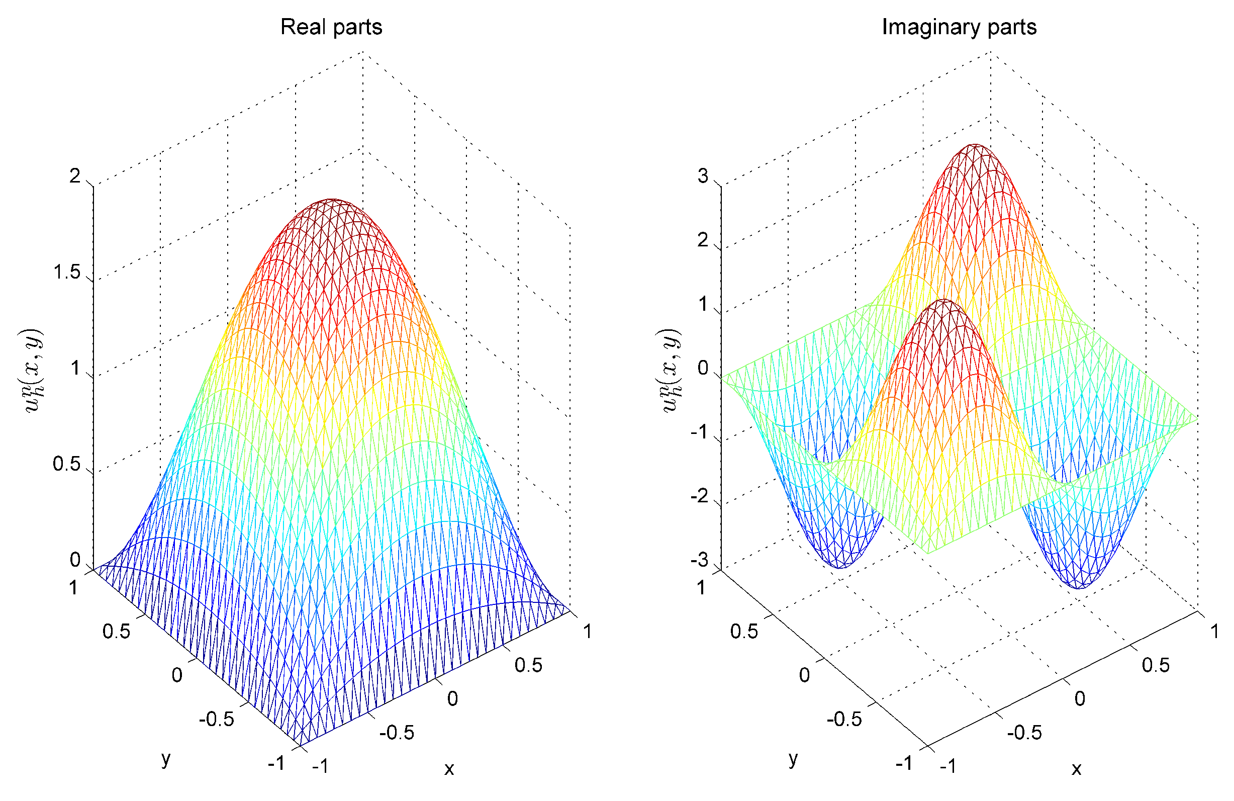
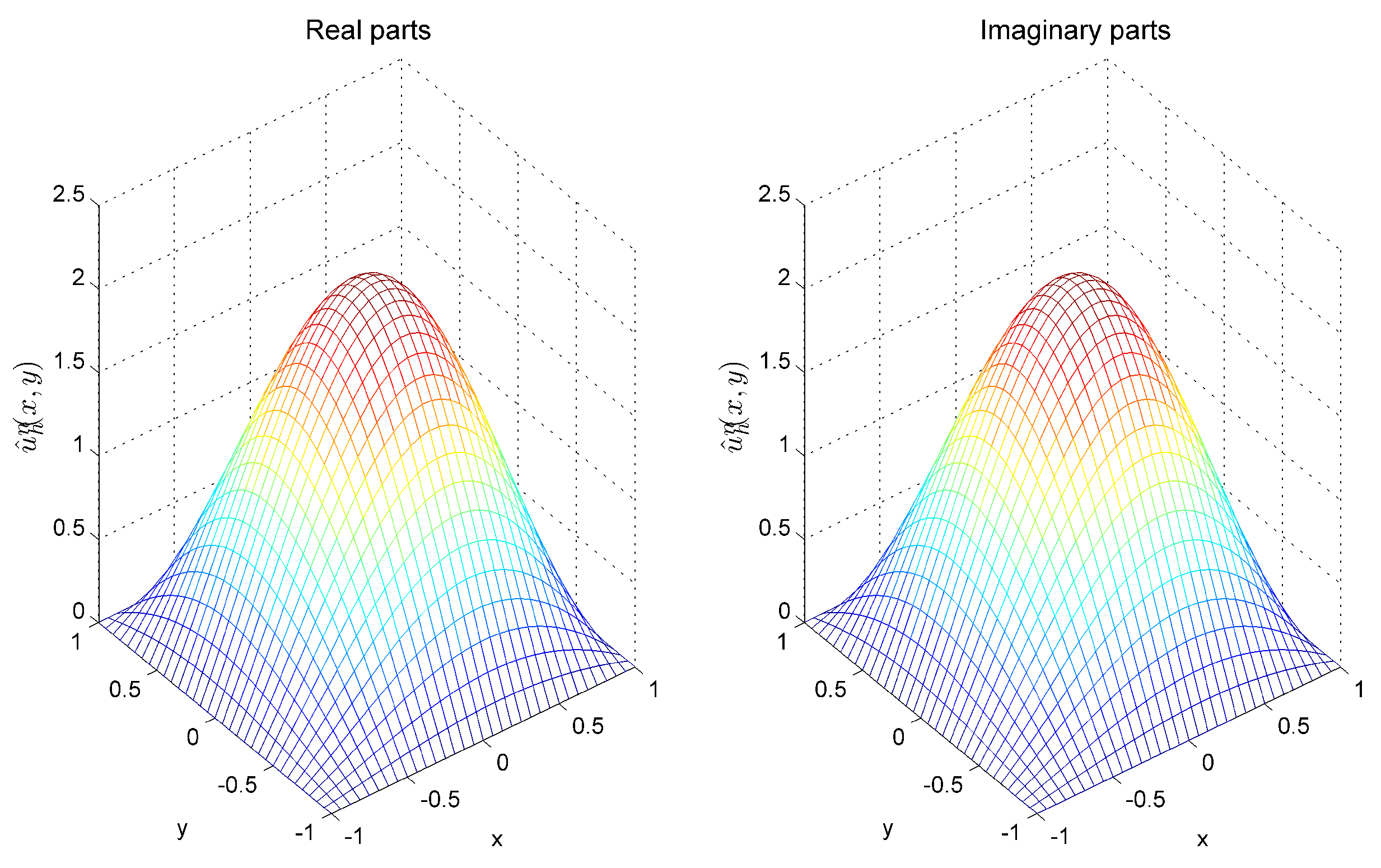
5. Numerical Examples

All simulations were carried out using MATLAB R2011a on a Windows server with Intel Core i5-8265 processor that possessed 8 GB RAM and a 1.60 GHz CPU.

Example 1

([25]). We consider the following linear Schrödinger equation:

$$\left\{\begin{array}{ccc}i{u}_t(\mathbf{x},t)=-\Delta u(\mathbf{x},t)+u(\mathbf{x},t)+f(\mathbf{x},t),\hfill & \hfill & (\mathbf{x},t)\in \Omega \times (0,1],\hfill \\ u(\mathbf{x},t)=0,\hfill & \hfill & (\mathbf{x},t)\in \partial \Omega \times (0,1],\hfill \\ u(\mathbf{x},0)=u_0(\mathbf{x}),\hfill & \hfill & \mathbf{x}\in \Omega ,\hfill \end{array}\right.$$

(53)

where $\Omega =[-1,1]\times [-1,1]$ and the function $f(\mathbf{x},t)$ is chosen corresponding to the exact solution

$u(x,y,t)=2t^4(1-x^2)(1-y^2)+i{e}^t$sin$(\pi (1+x))$sin$(\pi (1+y))$.

Let ${\Gamma }_H$ and ${\Gamma }_h$ be the quasi-uniform triangular partition of $\Omega$ with mesh sizes satisfying $h=H^2$. The linear finite element solution $u_h^n$ is computed by the back Euler fully discrete scheme, the two-grid solution ${\tilde{u}}_h^n$ is computed by Algorithm 1, and $U_h^n$ is the two-grid solution in [25]. The errors and CPU costs with respect to different times are listed in Table 1, Table 2, Table 3 and Table 4. We can see that the two-grid solution can achieve the same accuracy as the finite element solution and the two-grid method can save many CPU costs. In addition, the errors in the two-grid solution are less than those in [25]. The profiles of three solutions at $t=1.0$ on a $32\times 32$ mesh are plotted in Figure 1, Figure 2 and Figure 3.

Table 1. The error and CPU cost at t = 0.1 in the backward Euler scheme.

H	$\parallel {\mathit{u}}^{\mathit{n}}-{\mathit{u}}_{\mathit{h}}^{\mathit{n}}{\parallel }_1$	Order	Time (s)	$\parallel {\mathit{u}}^{\mathit{n}}-{\tilde{\mathit{u}}}_{\mathit{h}}^{\mathit{n}}{\parallel }_1$	Order	Time (s)	$\parallel {\mathit{u}}^{\mathit{n}}-{\mathit{U}}_{\mathit{h}}^{\mathit{n}}{\parallel }_1$
$1/4$	4.8118 × ${10}^{-1}$	/	1.01	5.5043× ${10}^{-1}$	/	0.022	5.6914 × ${10}^{-1}$
$1/8$	1.2050 × ${10}^{-1}$	1.00	26.2	1.3769 × ${10}^{-1}$	1.00	0.227	1.4358 × ${10}^{-1}$
$1/16$	3.0129 × ${10}^{-2}$	1.00	719	3.4431 × ${10}^{-2}$	1.00	5.13	3.5989 × ${10}^{-2}$

Table 2. The error and CPU cost t = 0.2 in the backward Euler scheme.

H	$\parallel {\mathit{u}}^{\mathit{n}}-{\mathit{u}}_{\mathit{h}}^{\mathit{n}}{\parallel }_1$	Order	Time (s)	$\parallel {\mathit{u}}^{\mathit{n}}-{\tilde{\mathit{u}}}_{\mathit{h}}^{\mathit{n}}{\parallel }_1$	Order	Time (s)	$\parallel {\mathit{u}}^{\mathit{n}}-{\mathit{U}}_{\mathit{h}}^{\mathit{n}}{\parallel }_1$
$1/4$	5.3163 × ${10}^{-1}$	/	1.81	5.8987 × ${10}^{-1}$	/	0.023	5.8826 × ${10}^{-1}$
$1/8$	1.3317 × ${10}^{-1}$	1.00	53.5	1.4885 × ${10}^{-1}$	0.99	0.235	1.4925 × ${10}^{-1}$
$1/16$	3.3300 × ${10}^{-2}$	1.00	1337	3.7389 × ${10}^{-2}$	1.00	5.21	3.7566 × ${10}^{-2}$

Table 3. The error and CPU cost at t = 0.5 in the backward Euler scheme.

H	$\parallel {\mathit{u}}^{\mathit{n}}-{\mathit{u}}_{\mathit{h}}^{\mathit{n}}{\parallel }_1$	Order	Time (s)	$\parallel {\mathit{u}}^{\mathit{n}}-{\tilde{\mathit{u}}}_{\mathit{h}}^{\mathit{n}}{\parallel }_1$	Order	Time (s)	$\parallel {\mathit{u}}^{\mathit{n}}-{\mathit{U}}_{\mathit{h}}^{\mathit{n}}{\parallel }_1$
$1/4$	7.1758 × ${10}^{-1}$	/	4.48	7.5505 × ${10}^{-1}$	/	0.024	7.8295 × ${10}^{-1}$
$1/8$	1.7980 × ${10}^{-1}$	1.00	128	1.8546 × ${10}^{-1}$	1.01	0.241	1.9261 × ${10}^{-1}$
$1/16$	4.4970 × ${10}^{-2}$	1.00	3769	4.6007 × ${10}^{-2}$	1.01	5.38	4.7613 × ${10}^{-2}$

Table 4. The error and CPU cost at t = 1.0 in the backward Euler scheme.

H	$\parallel {\mathit{u}}^{\mathit{n}}-{\mathit{u}}_{\mathit{h}}^{\mathit{n}}{\parallel }_1$	Order	Time (s)	$\parallel {\mathit{u}}^{\mathit{n}}-{\tilde{\mathit{u}}}_{\mathit{h}}^{\mathit{n}}{\parallel }_1$	Order	Time (s)	$\parallel {\mathit{u}}^{\mathit{n}}-{\mathit{U}}_{\mathit{h}}^{\mathit{n}}{\parallel }_1$
$1/4$	1.2075 × ${10}^0$	/	8.88	1.2310 × ${10}^0$	/	0.028	1.2626 × ${10}^0$
$1/8$	3.0266 × ${10}^{-1}$	1.00	253	3.0539 × ${10}^{-1}$	1.01	0.243	3.1258 × ${10}^{-1}$
$1/16$	7.6032 × ${10}^{-2}$	1.00	7551	7.6687 × ${10}^{-2}$	1.00	5.56	7.8453 × ${10}^{-2}$

Figure 1. The exact solution in the backward Euler scheme.

Figure 2. The finite element solution in the backward Euler scheme.

Figure 3. The two-grid solution in the backward Euler scheme.

Example 2

([26]). The function $f(\mathbf{x},t)$ in Equation (53) is chosen corresponding to the exact solution

$$u(x,y,t)=(1+i)e^t(1+x)(1+y)\sin (1-\mathrm{x})\sin (1-\mathrm{y}).$$

The domain $\Omega$ is uniformly divided into families ${\Gamma }_H$ and ${\Gamma }_h$ of rectangular meshes with $h=H^2$. The bilinear finite element solution $u_h^n$ is computed by the Crank–Nicolson fully discrete scheme, the two-grid solution ${\widehat{u}}_h^n$ is computed by Algorithm 2, and $U_h^n$ is the two-grid solution in [26]. The errors and CPU costs with respect to different times are listed in Table 5, Table 6, Table 7 and Table 8. It is obvious that errors in the two-grid solution are less than those in [26]. The profiles of three solutions at $t=1.0$ on a $32\times 32$ mesh are plotted in Figure 4, Figure 5 and Figure 6.

Table 5. The error and CPU cost at t = 0.1 in the Crank–Nicolson scheme.

H	$\parallel {\mathit{u}}^{\mathit{n}}-{\mathit{u}}_{\mathit{h}}^{\mathit{n}}{\parallel }_1$	Order	Time (s)	$\parallel {\mathit{u}}^{\mathit{n}}-{\widehat{\mathit{u}}}_{\mathit{h}}^{\mathit{n}}{\parallel }_1$	Order	Time (s)	$\parallel {\mathit{u}}^{\mathit{n}}-{\mathit{U}}_{\mathit{h}}^{\mathit{n}}{\parallel }_1$
$1/4$	8.6473 × ${10}^{-2}$	/	1.55	8.9016 × ${10}^{-2}$	/	1.23	8.9119 × ${10}^{-2}$
$1/8$	2.1611 × ${10}^{-2}$	1.00	29.7	2.2292 × ${10}^{-2}$	1.00	19.2	2.2318 × ${10}^{-2}$
$1/16$	5.4027 × ${10}^{-3}$	1.00	964	5.5751 × ${10}^{-3}$	1.00	606	5.5815 × ${10}^{-3}$

Table 6. The error and CPU cost t = 0.2 in the Crank–Nicolson scheme.

H	$\parallel {\mathit{u}}^{\mathit{n}}-{\mathit{u}}_{\mathit{h}}^{\mathit{n}}{\parallel }_1$	Order	Time (s)	$\parallel {\mathit{u}}^{\mathit{n}}-{\widehat{\mathit{u}}}_{\mathit{h}}^{\mathit{n}}{\parallel }_1$	Order	Time (s)	$\parallel {\mathit{u}}^{\mathit{n}}-{\mathit{U}}_{\mathit{h}}^{\mathit{n}}{\parallel }_1$
$1/4$	9.5565 × ${10}^{-2}$	/	3.15	1.0241 × ${10}^{-1}$	/	2.27	1.0288 × ${10}^{-1}$
$1/8$	2.3884 × ${10}^{-2}$	1.00	59.8	2.5708 × ${10}^{-2}$	1.00	38.7	2.5825 × ${10}^{-2}$
$1/16$	5.9709 × ${10}^{-3}$	1.00	2143	6.4347 × ${10}^{-3}$	1.00	1116	6.4640 × ${10}^{-3}$

Table 7. The error and CPU cost at t = 0.5 in the Crank–Nicolson scheme.

H	$\parallel {\mathit{u}}^{\mathit{n}}-{\mathit{u}}_{\mathit{h}}^{\mathit{n}}{\parallel }_1$	Order	Time (s)	$\parallel {\mathit{u}}^{\mathit{n}}-{\widehat{\mathit{u}}}_{\mathit{h}}^{\mathit{n}}{\parallel }_1$	Order	Time (s)	$\parallel {\mathit{u}}^{\mathit{n}}-{\mathit{U}}_{\mathit{h}}^{\mathit{n}}{\parallel }_1$
$1/4$	1.2901 × ${10}^{-1}$	/	7.51	1.4629 × ${10}^{-1}$	/	5.48	1.4890 × ${10}^{-1}$
$1/8$	3.2240 × ${10}^{-2}$	1.00	148	3.6766 × ${10}^{-2}$	1.00	118	3.7434 × ${10}^{-2}$
$1/16$	8.0599 × ${10}^{-3}$	1.00	5027	9.2073 × ${10}^{-3}$	1.00	2775	9.3754 × ${10}^{-3}$

Table 8. The error and CPU cost at t = 1.0 in the Crank–Nicolson scheme.

H	$\parallel {\mathit{u}}^{\mathit{n}}-{\mathit{u}}_{\mathit{h}}^{\mathit{n}}{\parallel }_1$	Order	Time (s)	$\parallel {\mathit{u}}^{\mathit{n}}-{\widehat{\mathit{u}}}_{\mathit{h}}^{\mathit{n}}{\parallel }_1$	Order	Time (s)	$\parallel {\mathit{u}}^{\mathit{n}}-{\mathit{U}}_{\mathit{h}}^{\mathit{n}}{\parallel }_1$
$1/4$	2.1268 × ${10}^{-1}$	/	14.9	2.2899 × ${10}^{-1}$	/	10.8	2.3462 × ${10}^{-1}$
$1/8$	5.3155 × ${10}^{-2}$	1.00	299	5.7344 × ${10}^{-2}$	1.00	239	5.8793 × ${10}^{-2}$
$1/16$	1.3289 × ${10}^{-2}$	1.00	9594	1.4342 × ${10}^{-2}$	1.00	5455	1.4708 × ${10}^{-2}$

Figure 4. The exact solution in the Crank–Nicolson scheme.

Figure 5. The finite element solution in the Crank–Nicolson scheme.

Figure 6. The two-grid solution in the Crank–Nicolson scheme.

6. Conclusions

In this paper, we have constructed a new two-grid algorithm in two fully discrete finite element schemes for the linear Schrödinger equation and have obtained error estimates of the exact solution with the two-grid solution. In the future, we will consider the two-grid algorithm of the finite element method for the nonlinear Schrödinger equation.

References

- Akrivis, G.D.; Dougalis, V.A.; Karakashian, O.A. On fully discrete Galerkin methods of second-order temporal accuracy for the nonlinear Schrödinger equation. Numer. Math. 1991, 59, 31–53. [Google Scholar] [CrossRef]
- Antonopoulou, D.C.; Karali, G.D.; Plexousakis, M.; Zouraris, G.E. Crank-Nicolson finite element discretizations for a two-dimensional linear Schrödinger-type equation posed in a noncylindrical domain. Math. Comp. 2015, 84, 1571–1598. [Google Scholar] [CrossRef]
- Li, M.; Gu, X.; Huang, C.; Fei, M.; Zhang, G. A fast linearized conservative finite element method for the strongly coupled nonlinear fractional Schrödinger equations. J. Comput. Phys. 2018, 358, 256–282. [Google Scholar] [CrossRef]
- Shi, D.; Wang, P.; Zhao, Y. Superconvergence analysis of anisotropic linear triangular finite element for nonlinear Schrödinger equation. Appl. Math. Lett. 2014, 38, 129–134. [Google Scholar] [CrossRef]
- Tian, Z.; Chen, Y.; Wang, J. Superconvergence analysis of bilinear finite element for the nonlinear Schrödinger equation on the rectangular mesh. Adv. Appl. Math. Mech. 2018, 10, 468–484. [Google Scholar] [CrossRef]
- Xu, J. A novel two-grid method for semilinear equations. SIAM J. Sci. Comput. 1994, 15, 231–237. [Google Scholar] [CrossRef]
- Xu, J. Two-grid discretization techniques for linear and nonlinear PDE. SIAM J. Numer. Anal. 1996, 33, 1759–1777. [Google Scholar] [CrossRef]
- Huang, Y.; Chen, Y. A multi-level iterative method for solving finite element equations of nonlinear singular two-point boundary value problems. Nat. Sci. J. Xiangtan Univ. 1994, 16, 23–26. (In Chinese) [Google Scholar]
- Xu, J.; Zhou, A. Local and parallel finite element algorithms based on two-grid discretizations. Math. Comp. 2000, 69, 881–909. [Google Scholar] [CrossRef]
- Bi, C.; Wang, C.; Lin, Y. A posteriori error estimates of two-grid finite element methods for nonlinear elliptic problems. J. Sci. Comput. 2018, 74, 23–48. [Google Scholar] [CrossRef]
- Dawson, C.N.; Wheeler, M.F. Two-grid method for mixed finite element approximations of non-linear parabolic equations. Contemp. Math. 1994, 180, 191–203. [Google Scholar]
- Chen, Y.; Luan, P.; Lu, Z. Analysis of two-grid methods for nonlinear parabolic equations by expanded mixed finite element methods. Adv. Appl. Math. Mech. 2009, 1, 830–844. [Google Scholar] [CrossRef]
- Chen, C.; Yang, M.; Bi, C. Two-grid methods for finite volume element approximations of nonlinear parabolic equations. J. Comput. Appl. Math. 2009, 228, 123–132. [Google Scholar] [CrossRef]
- Shi, D.; Yang, H. Unconditional optimal error estimates of a two-grid method for semilinear parabolic equation. Appl. Math. Comput. 2017, 310, 40–47. [Google Scholar] [CrossRef]
- Chen, L.; Chen, Y. Two-grid method for nonlinear reaction-diffusion equations by mixed finite element methods. J. Sci. Comput. 2011, 49, 383–401. [Google Scholar] [CrossRef]
- Chen, Y.; Huang, Y.; Yu, D. A two-grid method for expanded mixed finite-element solution of semilinear reaction-diffusion equations. Int. J. Numer. Meth. Eng. 2003, 57, 193–209. [Google Scholar] [CrossRef]
- Chen, Y.; Hu, H. Two-grid method for miscible displacement problem by mixed finite element methods and mixed finite element method of characteristics. Commun. Comput. Phys. 2016, 19, 1503–1528. [Google Scholar] [CrossRef]
- Chen, Y.; Zeng, J.; Zhou, J. Lp error estimates of two-grid method for miscible displacement problem. J. Sci. Comput. 2016, 69, 28–51. [Google Scholar] [CrossRef]
- Zhong, L.; Liu, C.; Shu, S. Two-level additive preconditioners for edge element discretizations of time-harmonic Maxwell equations. Comput. Math. Appl. 2013, 66, 432–440. [Google Scholar] [CrossRef]
- Zhou, J.; Hu, X.; Zhong, L.; Shu, S.; Chen, L. Two-grid methods for Maxwell eigenvalue problems. SIAM J. Numer. Anal. 2014, 52, 2027–2047. [Google Scholar] [CrossRef]
- Jin, J.; Shu, S.; Xu, J. A two-grid discretization method for decoupling systems of partial differential equations. Math. Comp. 2006, 75, 1617–1626. [Google Scholar] [CrossRef]
- Chien, C.S.; Huang, H.T.; Jeng, B.W.; Li, Z.C. Two-grid discretization schemes for nonlinear Schrödinger equations. J. Comput. Appl. Math. 2008, 214, 549–571. [Google Scholar] [CrossRef]
- Wu, L. Two-grid mixed finite-element methods for nonlinear Schrödinger equations. Numer. Methods Partial. Differ. Equ. 2012, 28, 63–73. [Google Scholar] [CrossRef]
- Hu, H. Two-grid method for two-dimensional nonlinear Schrödinger equation by mixed finite element method. Comput. Math. Appl. 2018, 75, 900–917. [Google Scholar] [CrossRef]
- Tian, Z.; Chen, Y.; Huang, Y.; Wang, J. Two-grid method for the two-dimensional time-dependent Schrödinger equation by the finite element method. Comput. Math. Appl. 2019, 77, 3043–3053. [Google Scholar] [CrossRef]
- Wang, J.; Jin, J.; Tian, Z. Two-grid finite element method with Crank-Nicolson fully discrete scheme for the time-dependent Schrödinger equation. Numer. Math. Theor. Meth. Appl. 2020, 13, 334–352. [Google Scholar]