The Second-Order Numerical Approximation for a Modified Ericksen–Leslie Model

Abstract

In this study, two numerical schemes with second-order accuracy in time for a modified Ericksen–Leslie model are constructed. The highlight is based on a novel convex splitting method for dealing with the nonlinear potentials, which is integrated with the second-order backward differentiation formula (BDF2) and leap frog method for temporal discretization and the finite element method for spatial discretization. The unconditional energy stability of both schemes is further demonstrated. Finally, several numerical examples are presented to demonstrate the efficiency and accuracy of the proposed schemes.

1. Introduction

Liquid crystal is typically viewed as a state of matter that is distinct from the solid, liquid, and gaseous states. This is due to the fact that liquid crystal is an intermediate phase between a liquid and a solid. It can flow like a liquid, but it also exhibits a partial order in the mesoscopic scale of the solid phase, which is normally due to its anisotropic microstructures. According to the degree of positional or orientational ordering shown by the molecules, different degrees of ordering can be achieved, which depends on the temperature and the concentration of the solute in the solvent. The nematic phase is considered the simplest liquid crystal phase; it is composed of elongated rod-like molecules with similar sizes. Its centers of mass have no positional order in an isotropic liquid, but they tend to align along certain locally preferred directions and confer an anisotropic structure. In recent years, the hydrodynamic systems that describe the motion of nematic liquid crystals have become more important in technology. Readers are referred to [1] for a review of dynamic phenomena in liquid crystal materials.

To the best of our knowledge, the famous continuum theory for flows of liquid crystal was first initiated by Oseen and then developed mainly by Eriksen and Leslie [2,3,4,5]. As far as liquid crystal is concerned, there are a large number of works in the literature dedicated to diverse features of a system modeling the dynamics of the nematic liquid crystal flows—the so called Ericksen–Leslie model. The Ericksen–Leslie model describes the fluid dynamics of nematic liquid crystals, and it is a coupling between the Navier–Stokes system and the Ginzburg–Landau equations. This system has been investigated widely from various perspectives [6,7,8,9,10].

The Ericksen–Leslie model is a strongly nonlinear coupled system. Due to its complexity, exact solutions of this system are extremely rare. Numerical methods are an important tool for solving these highly nonlinear systems. Consequently, our interest is in constructing numerical approximations for the Ericksen–Leslie model. Lin and Liu [11] developed an extremely significant discovery, which is the existence of energy estimates for the simplified Ericksen–Leslie equations. Liu and Walkington [8] demonstrated implicit Euler time stepping and the finite element approximation in the spatial domain. Lin and Liu [12] discussed a splitting scheme combined with a fixed-point iterative method, which largely reduced the computational time. F.M. Guillen-Gonzalez and J.V. Gutierrez-Santacreu [13] introduced a linear semi-implicit scheme for the Ericksen–Leslie system. V. Girault and F. Guillen-Gonzalez [14] presented a decoupling algorithm. The above papers were all first-order accurate in time for the Ericksen–Leslie system. Then, Santiago, B. et al. [15] proposed a Crank–Nicolson time integration scheme that was unconditionally stable, preserving the energy law. Bao et al. [16] considered a time discretization scheme of a simplified system that preserved spherical constraints at each node, had a discrete energy law, and led to a linear and decoupled elliptic equation solution at each time step. Wang et al. [17] considered a numerical scheme with a second-order backward differentiation formula (BDF) by combining the Lagrange multiplier method and the pressure correction strategy. Cheng et al. [18] proposed and analyzed a first-order exact time difference scheme for the Ericksen–Leslie system. Recently, Wang et al. [19] constructed a first-order sphere-constraint-preserving numerical scheme for the variable-density Ericksen–Leslie equation, and they derived the unconditional energy stability and strict time error estimates. Miao et al. [20] proposed a numerical scheme of the second-order backward differential formula (BDF) for the Ericksen–Leslie model of nematic liquid crystal by combining the convex splitting method and the pressure correction strategy, and this was unconditionally stable in terms of energy. Zhang et al. [10] constructed a second-order numerical scheme with the advantages of complete decoupling, linearization, and unconditional stability of energy in order to numerically approximate the penalized Ericksen–Leslie equations. As far as we know, the second-order numerical method is more accurate than the first-order one in time. So, we developed two second-order time-accurate schemes for the Ericksen–Leslie model in this study. For the backward differentiation formula scheme, this study applied the pressure-correction [21,22] strategy to decouple the pressure from the velocity in order to reduce the computational cost. Then, the leap frog scheme is proposed for the coupling system. It is worth noting that algorithm development is a significant point for the highly complex coupled and nonlinear characteristics.

It is obvious that one of the difficulties in numerically resolving the nonlinear-phase field model is expediently dealing with the nonlinear term in the model. We review some methods for dealing with the potential function, such as the invariant energy quadratization (IEQ) method, the scalar auxiliary variable (SAV) method, the Lagrange multiplier method, and the convex splitting method. Yang [23] mentioned the invariant energy quadratization (IEQ) method, which can be applied to a large number of free energies for phase field models. Shen et al. [24,25] introduced the scalar auxiliary variable method (SAV) for gradient flows, and it is an insufficient case that a scalar auxiliary variable only depends on the time variable. F. Guillen-Gonzalez and G. Tierra [26] presented a linear unconditionally stable scheme for the Cahn–Hilliard equation based on the Lagrange multiplier method. There is the convex splitting method [27,28], which treats the convex part of the potential function implicitly and the concave part explicitly. It was first proposed by Elliott and Stuart [29] and developed by Eyre [30] to solve phase flow equations and nematic liquid crystal flows. However, the IEQ method and SAV method involve more complicated variable coefficients in comparison with the Lagrange multiplier method of linearizing nonlinear potential. The introduction of the Lagrange multiplier and the convex splitting method are extremely common methods, and they are usually used to solve the Cahn–Hilliard equations with double-well potential. For the Ericksen–Leslie model, this study shows a novel convex splitting method for dealing with the penalty term. There has been no recent theoretical or numerical analysis.

The rest of this paper is organized as follows. In Section 2, we briefly discuss the modified Ericksen–Leslie model and the energy dissipation law of the model. In Section 3, fully discrete numerical schemes are constructed, and we prove that the second-order backward differentiation formula and the leap frog scheme satisfy unconditional energy stability. In Section 4, several numerical experiments are carried out to confirm the numerical accuracy and defect dynamics of liquid crystals. We give some concluding remarks in the last section.

2. The Model and Its Energy Law

Some notations are given here. We assume that $\mathrm{\Omega }\in {\mathbb{R}}^d$ (dimension d = 2, 3) is an open and bounded domain with a smooth boundary $\partial \mathrm{\Omega }$. For scalar functions u and v and vector functions $\mathbf{u}=(u_1,u_2)$ and $\mathbf{v}=(v_1,v_2)$, we can define the $L^2$ inner product and norm as follows:

$$\begin{array}{cc}\hfill & (u,v)={\int }_{\mathrm{\Omega }}uvdx,{\parallel u\parallel }^2=(u,u),\hfill \\ \hfill & (\mathbf{u},\mathbf{v})={\int }_{\mathrm{\Omega }}\mathbf{u}{\mathbf{v}}^{T}d\mathbf{x}=\sum _{i=1}^n{\int }_{\mathrm{\Omega }}{u}_i{v}_{i}d\mathbf{x},{\parallel \mathbf{u}\parallel }^2=(\mathbf{u},\mathbf{u}).\hfill \end{array}$$

We provide a brief introduction to the modified Ericksen–Leslie model [31]. We define $Q=(0,T)\times \mathrm{\Omega }$; $\mathbf{u}:\mathrm{\Omega }\to R^2$ is the unknown velocity field, and $\mathbf{d}:\mathrm{\Omega }\to R^2$ is the preferential orientation vector of molecules. The total energy E reads as follows:

$$\begin{array}{c}\hfill E=E_{kin}+E_{ela},\end{array}$$

(1)

where $E_{kin}$ is the kinetic energy and $E_{ela}$ is the elastic energy, and they are, respectively, given in the following:

$$\begin{array}{cc}\hfill & E_{kin}=\frac{1}{2}{\int }_{\mathrm{\Omega }}\mid \mathbf{u}{\mid }^{2}dx,E_{ela}={\int }_{\mathrm{\Omega }}\frac{\lambda }{2}\mid \nabla \mathbf{d}{\mid }^2+\lambda F(\mathbf{d})dx.\hfill \end{array}$$

(2)

Here, $F(\mathbf{d})=\frac{1}{4{ϵ}^2}{(\mid \mathbf{d}{\mid }^2-1)}^2$ is the Ginzburg–Landau potential [32], and $ϵ$ is a model parameter measuring the size of the defect core.

The modified Ericksen–Leslie model reads as follows:

$$\begin{array}{c}\hfill \begin{array}{cc}\hfill & {\partial }_t\mathbf{d}+\mathbf{u}·\nabla \mathbf{d}=\gamma \mathbf{h},inQ,\hfill \\ \hfill & \mathbf{h}=∆\mathbf{d}-f(\mathbf{d})inQ,\hfill \\ \hfill & {\partial }_t\mathbf{u}+\mathbf{u}·\nabla \mathbf{u}=\eta ∆\mathbf{u}-\nabla p-\lambda \mathbf{h}\nabla \mathbf{d},inQ,\hfill \\ \hfill & \nabla ·\mathbf{u}=0,inQ.\hfill \end{array}\end{array}$$

(3)

Here, $\mathbf{h}=-\frac{\delta E}{\delta \mathbf{d}}$ is the molecular field, p is the pressure, $f(\mathbf{d})=F^{\prime }(\mathbf{d})=\frac{1}{{ϵ}^2}({\mathbf{d}}^3-\mathbf{d})$, $\eta$ is dimensionless and is for the viscosity, $\gamma$ is the relaxation time parameter, and $\lambda$ is the elastic parameter. We consider the following boundary conditions:

$$\begin{array}{cc}\hfill & \mathbf{u}{\mid }_{\partial \mathrm{\Omega }}=0,\mathbf{n}·\nabla \mathbf{d}=0,\hfill \end{array}$$

(4)

where $\mathbf{n}$ is the unit outward normal of the domain $\mathrm{\Omega }$. The initial conditions are

$$\begin{array}{c}\hfill \mathbf{d}(\mathbf{x},0)={\mathbf{d}}_0,\mathbf{u}(\mathbf{x},0)={\mathbf{u}}_0,\varphi (\mathbf{x},0)={\varphi }_0,\mathbf{x}\in \mathrm{\Omega }.\end{array}$$

(5)

Remark 1.

This study uses the convex splitting strategy to develop new schemes for the modified Ericksen–Leslie model. The traditional convex splitting strategy refers to treating the convex part of the potential function implicitly and the concave part explicitly, that is, $g(\mathbf{d})=g_1(\mathbf{d})+g_2(\mathbf{d})=\frac{1}{{ϵ}^2}{\mathbf{d}}^3-\frac{1}{{ϵ}^2}\mathbf{d}$. However, the potential function $F(\mathbf{d})$ in this study can be split into the following convex function and concave function, respectively:

$$\begin{array}{c}\hfill F_1(\mathbf{d})=\frac{1}{{ϵ}^2}({\mathbf{d}}^2+\frac{1}{4}),F_2(\mathbf{d})=\frac{1}{{ϵ}^2}(\frac{1}{4}{\mathbf{d}}^4-\frac{3}{2}{\mathbf{d}}^2).\end{array}$$

Correspondingly,

$$\begin{array}{c}\hfill f_1(\mathbf{d})=\frac{2}{{ϵ}^2}\mathbf{d},f_2(\mathbf{d})=\frac{1}{{ϵ}^2}({\mathbf{d}}^3-3\mathbf{d}).\end{array}$$

3. Numerical Schemes

3.1. The Backward Differentiation Formula Scheme

Let $S_h$ be a set of triangulations of $\mathrm{\Omega }$ with $\overline{\mathrm{\Omega }}={\cup }_{k\in S_h}k$, where $h\to 0$ is assumed to be uniformly regular. Here, $h=\underset{k\in S_h}{sup}diam(k)$. We denote the finite element spaces $X_h\in X,Y_h\in Y$. Then, the discrete divergence-free space $V_h$ is given by $V_h=\{v_h\in X_h:(\nabla ·v_h,r_h)=0,\forall r_h\in R_h\}$. The pressure stability relies on the inf-sup condition. There exists $\beta >0$ with no restriction of the mesh grid size h such that $\underset{r_h\in R_h}{inf}\underset{v_h\in V_h}{sup}{\displaystyle \frac{(r_h,\nabla ·v_h)}{\parallel r_h{\parallel }_0{\parallel v_h\parallel }_1}}\ge \beta$. The strategy of pressure correction is the time-marching method, which is composed of two steps. In the first step, the pressure is treated explicitly or ignored. In the second step, the pressure is projected by the former velocity onto the space $V_h$. A pressure-correction scheme is used to decouple the computation of the pressure from that of the velocity. Let N be a positive integer, let the time interval $[0,T]$ be uniformly dissected with $0=t_0<t_1<∆<t_N=T$, and let the time nodes satisfy $t_i=i\tau (i=0,1,∆,N);\tau$ is the time step. For $n\ge 1$, the numerical scheme reads as follows:

• Scheme I Step 1. Given $({\mathbf{d}}_h^{n-1},{\mathbf{d}}_h^n,{\mathbf{u}}_h^{n-1},{\mathbf{u}}_h^n,p_h^n)\in V_h\times V_h\times V_h\times V_h\times Y_h$, find $({\mathbf{d}}_h^{n+1},{\tilde{\mathbf{u}}}_h^{n+1})$$\in (V_h\times V_h)$ as the solution of

  $$\begin{array}{cc}\hfill & D_{\tau }{\mathbf{d}}_h^{n+1}+{\tilde{\mathbf{u}}}_h^{n+1}·\nabla {\widehat{\mathbf{d}}}_h^{n+1}=\gamma {\mathbf{h}}_h^{n+1},\hfill \end{array}$$

  (6)

  $$\begin{array}{cc}\hfill & {\mathbf{h}}_h^{n+1}-∆{\mathbf{d}}_h^{n+1}+f_1({\mathbf{d}}_h^{n+1})+f_2({\mathbf{d}}_h^{n+1},{\widehat{\mathbf{d}}}_h^{n+1})=0,\hfill \end{array}$$

  (7)

  $$\begin{array}{cc}\hfill & D_{\tau }{\tilde{\mathbf{u}}}_h^{n+1}+{\widehat{\mathbf{u}}}_h^{n+1}·\nabla {\tilde{\mathbf{u}}}_h^{n+1}=-\nabla p_h^n+\eta ∆{\tilde{\mathbf{u}}}_h^{n+1}-\lambda {\mathbf{h}}_h^{n+1}\nabla {\widehat{\mathbf{d}}}_h^{n+1},\hfill \end{array}$$

  (8)

  $$\begin{array}{cc}\hfill & {\tilde{\mathbf{u}}}_h^{n+1}{\mid }_{\partial \mathrm{\Omega }}=0,\frac{\partial {\mathbf{d}}_h^{n+1}}{\partial \mathbf{n}}{\mid }_{\partial \mathrm{\Omega }}=0.\hfill \end{array}$$

  (9)

Step 2. Given $({\tilde{\mathbf{u}}}_h^{n+1},p_h^n)\in V_h\times Y_h$, find $({\mathbf{u}}_h^{n+1},p_h^{n+1})\in (V_h\times Y_h)$ as the solution of

$$\begin{array}{cc}\hfill & 3\frac{{\mathbf{u}}_h^{n+1}-{\tilde{\mathbf{u}}}_h^{n+1}}{2\tau }+\nabla (p_h^{n+1}-p_h^n)=0,\hfill \end{array}$$

(10)

$$\begin{array}{cc}\hfill & \nabla ·{\mathbf{u}}_h^{n+1}=0,\hfill \end{array}$$

(11)

where $D_{\tau }{\mathbf{d}}_h^{n+1}={\displaystyle \frac{3{\mathbf{d}}_h^{n+1}-4{\mathbf{d}}_h^n+{\mathbf{d}}_h^{n-1}}{2\tau }}$, $D_{\tau }{\tilde{\mathbf{u}}}_h^{n+1}={\displaystyle \frac{3{\tilde{\mathbf{u}}}_h^{n+1}-4{\mathbf{u}}_h^n+{\mathbf{u}}_h^{n-1}}{2\tau }}$,

• $D_{\tau }{\mathbf{u}}_h^{n+1}={\displaystyle \frac{3{\mathbf{u}}_h^{n+1}-4{\mathbf{u}}_h^n+{\mathbf{u}}_h^{n-1}}{2\tau }}$, ${\widehat{\mathbf{d}}}_h^{n+1}=2{\mathbf{d}}_h^n-{\mathbf{d}}_h^{n-1}$, ${\widehat{\mathbf{u}}}_h^{n+1}=2{\mathbf{u}}_h^n-{\mathbf{u}}_h^{n-1}$,
• $f_1({\mathbf{d}}_h^{n+1})={\displaystyle \frac{2}{{ϵ}^2}}{\mathbf{d}}_h^{n+1}$, $f_2({\mathbf{d}}_h^{n+1},{\widehat{\mathbf{d}}}_h^{n+1})={\displaystyle \frac{1}{{ϵ}^2}}({({\widehat{\mathbf{d}}}_h^{n+1})}^2{\mathbf{d}}_h^{n+1}-3{\widehat{\mathbf{d}}}_h^{n+1})$.

For n = 1, given ${\mathbf{u}}_h^0,p_h^0,{\mathbf{d}}_h^0$, find ${\mathbf{u}}_h^1,{\mathbf{d}}_h^1,p_h^1$ as the solution of

$$\begin{array}{cc}\hfill & \frac{{\mathbf{d}}_h^1-{\mathbf{d}}_h^0}{\tau }+{\mathbf{u}}_h^1·\nabla {\mathbf{d}}_h^0=\gamma {\mathbf{h}}_h^1,\hfill \\ \hfill & {\mathbf{h}}_h^1=∆{\mathbf{d}}_h^1-(f_1({\mathbf{d}}_h^1)+f_2({\mathbf{d}}_h^1,{\mathbf{d}}_h^0)),\hfill \\ \hfill & \frac{{\mathbf{u}}_h^1-{\mathbf{u}}_h^0}{\tau }+{\mathbf{u}}_h^0·\nabla {\mathbf{u}}_h^1=-\nabla p_h^1+\eta ∆{\mathbf{u}}_h^1-\lambda {\mathbf{h}}_h^1\nabla {\mathbf{d}}_h^0,\hfill \\ \hfill & {\mathbf{u}}_h^1{\mid }_{\partial \mathrm{\Omega }}=0,\frac{\partial {\mathbf{d}}_h^1}{\partial \mathbf{n}}{\mid }_{\partial \mathrm{\Omega }}=0,\hfill \\ \hfill & \nabla ·{\mathbf{u}}_h^1=0.\hfill \end{array}$$

(12)

Now, we prove that Scheme I is unconditionally stable in terms of energy.

Theorem 1

(Energy Stability). Scheme I satisfies the discrete energy dissipation law as follows:

$$\begin{array}{c}\hfill \begin{array}{cc}\hfill & \frac{1}{\tau }({\mathrm{\Xi }}^{n+1}-{\mathrm{\Xi }}^n)\le -2\eta \parallel \nabla {\tilde{\mathbf{u}}}_h^{n+1}{\parallel }^2-2\lambda \gamma {\parallel {\mathbf{h}}_h^{n+1}\parallel }^2\le 0,\hfill \end{array}\end{array}$$

(13)

where

$$\begin{array}{c}\hfill \begin{array}{cc}\hfill {\mathrm{\Xi }}^{n+1}=& E^{n+1}+{\displaystyle \frac{1}{2}}\parallel 2{\mathbf{u}}_h^{n+1}-{\mathbf{u}}_h^n{\parallel }^2+{\displaystyle \frac{\lambda }{2}}{\parallel 2\nabla {\mathbf{d}}_h^{n+1}-\nabla {\mathbf{d}}_h^n\parallel }^2\hfill \\ \hfill & +{\displaystyle \frac{\lambda }{{ϵ}^2}}\parallel 2{\mathbf{d}}_h^{n+1}-{\mathbf{d}}_h^n{\parallel }^2+{\displaystyle \frac{\lambda }{2{ϵ}^2}}{\parallel {\widehat{\mathbf{d}}}_h^{n+1}(2{\mathbf{d}}_h^{n+1}-{\mathbf{d}}_h^n)\parallel }^2\hfill \\ \hfill & +{\displaystyle \frac{9\lambda }{2{ϵ}^2}}(1-\parallel {\mathbf{d}}_h^{n+1}{\parallel }^2)+{\displaystyle \frac{2{\tau }^2}{3}}{\parallel \nabla p_h^{n+1}\parallel }^2,\hfill \\ \hfill E^{n+1}=& \frac{1}{2}\parallel {\mathbf{u}}_h^{n+1}{\parallel }^2+{\displaystyle \frac{\lambda }{2}}\parallel \nabla {\mathbf{d}}_h^{n+1}{\parallel }^2+{\displaystyle \frac{\lambda }{4{ϵ}^2}}(\parallel {\mathbf{d}}_h^{n+1}{{\parallel }^2-1)}^2.\hfill \end{array}\end{array}$$

(14)

Proof. 

For (8), we take the inner product with ${\tilde{\mathbf{u}}}_h^{n+1}$ in $L^2$ to obtain

$$\begin{array}{c}\hfill \begin{array}{cc}\hfill & (D_{\tau }{\tilde{\mathbf{u}}}_h^{n+1},{\tilde{\mathbf{u}}}_h^{n+1})+({\widehat{\mathbf{u}}}_h^{n+1}·\nabla {\tilde{\mathbf{u}}}_h^{n+1},{\tilde{\mathbf{u}}}_h^{n+1})-(p_h^n,\nabla ·{\tilde{\mathbf{u}}}_h^{n+1})\hfill \\ \hfill & +\eta (\nabla {\tilde{\mathbf{u}}}_h^{n+1},\nabla {\tilde{\mathbf{u}}}_h^{n+1})=-\lambda ({\mathbf{h}}_h^{n+1}\nabla {\widehat{\mathbf{d}}}_h^{n+1},{\tilde{\mathbf{u}}}_h^{n+1}).\hfill \end{array}\end{array}$$

(15)

Then, we put (6) into the right part of (15) to get

$$\begin{array}{c}\hfill \begin{array}{cc}\hfill \lambda ({\mathbf{h}}_h^{n+1},{\tilde{\mathbf{u}}}_h^{n+1}·\nabla {\widehat{\mathbf{d}}}_h^{n+1})& =\lambda ({\mathbf{h}}_h^{n+1},\gamma ({\mathbf{h}}_h^{n+1}-D_{\tau }{\mathbf{d}}_h^{n+1}))\hfill \\ \hfill & =\lambda \gamma \parallel {\mathbf{h}}_h^{n+1}{\parallel }^2-\lambda ({\mathbf{h}}_h^{n+1},D_{\tau }{\mathbf{d}}_h^{n+1}).\hfill \end{array}\end{array}$$

(16)

Besides, we put (16) into (15) to get

$$\begin{array}{c}\hfill \begin{array}{cc}\hfill & (D_{\tau }{\tilde{\mathbf{u}}}_h^{n+1},{\tilde{\mathbf{u}}}_h^{n+1})+\eta \parallel \nabla {\tilde{\mathbf{u}}}_h^{n+1}{\parallel }^2+\lambda \gamma {\parallel {\mathbf{h}}_h^{n+1}\parallel }^2=\lambda ({\mathbf{h}}_h^{n+1},D_{\tau }{\mathbf{d}}_h^{n+1}).\hfill \end{array}\end{array}$$

(17)

For (7), we take the inner product with $\lambda D_{\tau }{\mathbf{d}}_h^{n+1}$ in $L^2$ to get

$$\begin{array}{c}\hfill \begin{array}{cc}\hfill & \lambda ({\mathbf{h}}_h^{n+1},D_{\tau }{\mathbf{d}}_h^{n+1})+\lambda (\nabla {\mathbf{d}}_h^{n+1},\nabla D_{\tau }{\mathbf{d}}_h^{n+1})+\lambda (f_1({\mathbf{d}}_h^{n+1},D_{\tau }{\mathbf{d}}_h^{n+1})\hfill \\ \hfill & +\lambda (f_2({\mathbf{d}}_h^{n+1},{\widehat{\mathbf{d}}}_h^{n+1}),D_{\tau }{\mathbf{d}}_h^{n+1})=0.\hfill \end{array}\end{array}$$

(18)

Due to

$$\begin{array}{c}\hfill \begin{array}{cc}\hfill (f_1({\mathbf{d}}_h^{n+1}),D_{\tau }{\mathbf{d}}_h^{n+1})=& \frac{1}{2\tau {ϵ}^2}(\parallel {\mathbf{d}}_h^{n+1}{\parallel }^2-\parallel {\mathbf{d}}_h^n{\parallel }^2+{\parallel 2{\mathbf{d}}_h^{n+1}-{\mathbf{d}}_h^n\parallel }^2\hfill \\ \hfill & -\parallel 2{\mathbf{d}}_h^n-{\mathbf{d}}_h^{n-1}{\parallel }^2+\parallel {\mathbf{d}}_h^{n+1}-2{\mathbf{d}}_h^n+{\mathbf{d}}_h^{n-1}{\parallel }^2),\hfill \end{array}\end{array}$$

(19)

we derive

$$\begin{array}{cc}\hfill & (f_2({\mathbf{d}}_h^{n+1},{\widehat{\mathbf{d}}}_h^{n+1}),D_{\tau }{\mathbf{d}}_h^{n+1})={\displaystyle \frac{1}{{ϵ}^2}}({({\widehat{\mathbf{d}}}_h^{n+1})}^2{\mathbf{d}}_h^{n+1}-3{\widehat{\mathbf{d}}}_h^{n+1}),D_{\tau }{\mathbf{d}}_h^{n+1})\hfill \\ \hfill =& \frac{1}{2\tau {ϵ}^2}({\int }_{\mathrm{\Omega }}\frac{1}{2}{({\widehat{\mathbf{d}}}_h^{n+1})}^2[{({\mathbf{d}}_h^{n+1})}^2-{({\mathbf{d}}_h^n)}^2+{(2{\mathbf{d}}_h^{n+1}-{\mathbf{d}}_h^n)}^2-{(2{\mathbf{d}}_h^n-{\mathbf{d}}_h^{n-1})}^2\hfill \\ \hfill & +{({\mathbf{d}}_h^{n+1}-2{\mathbf{d}}_h^n+{\mathbf{d}}_h^{n-1})}^2]d\mathbf{x}+3(-\frac{1}{2}(\parallel {\mathbf{d}}_h^{n+1}{\parallel }^2+{\parallel 2{\mathbf{d}}_h^{n+1}-{\mathbf{d}}_h^n\parallel }^2\hfill \\ \hfill & -2\parallel {\mathbf{d}}_h^{n+1}-{\mathbf{d}}_h^n{\parallel }^2)+\frac{1}{2}(\parallel {\mathbf{d}}_h^n{\parallel }^2-\parallel 2{\mathbf{d}}_h^n-{\mathbf{d}}_h^{n-1}{\parallel }^2-2\parallel {\mathbf{d}}_h^n-{\mathbf{d}}_h^{n-1}{\parallel }^2))\hfill \\ \hfill & +\frac{3}{2}\parallel {\mathbf{d}}_h^{n+1}-2{\mathbf{d}}_h^n+{\mathbf{d}}_h^{n-1}{\parallel }^2)\hfill \\ \hfill =& \frac{1}{4\tau {ϵ}^2}(\parallel {\widehat{\mathbf{d}}}_h^{n+1}{\mathbf{d}}_h^{n+1}{\parallel }^2-\parallel {\widehat{\mathbf{d}}}_h^{n+1}{\mathbf{d}}_h^n{\parallel }^2+{\parallel {\widehat{\mathbf{d}}}_h^{n+1}(2{\mathbf{d}}_h^{n+1}-{\mathbf{d}}_h^n)\parallel }^2\hfill \\ \hfill & -\parallel {\widehat{\mathbf{d}}}_h^{n+1}(2{\mathbf{d}}_h^n-{\mathbf{d}}_h^{n-1}){\parallel }^2+\parallel ({\widehat{\mathbf{d}}}_h^{n+1}({\mathbf{d}}_h^{n+1}-2{\mathbf{d}}_h^n+{\mathbf{d}}_h^{n-1}){\parallel }^2)\hfill \\ \hfill & +\frac{3}{2\tau {ϵ}^2}(-\frac{1}{2}(\parallel {\mathbf{d}}_h^{n+1}{\parallel }^2+4\parallel {\mathbf{d}}_h^{n+1}{\parallel }^2+\parallel {\mathbf{d}}_h^n{\parallel }^2-4{\mathbf{d}}_h^{n+1}{\mathbf{d}}_h^n-2{\parallel {\mathbf{d}}_h^{n+1}\parallel }^2\hfill \\ \hfill & -2\parallel {\mathbf{d}}_h^n{\parallel }^2+4{\mathbf{d}}_h^{n+1}{\mathbf{d}}_h^n)+\frac{1}{2}(\parallel {\mathbf{d}}_h^n{\parallel }^2+4\parallel {\mathbf{d}}_h^n{\parallel }^2+{\parallel {\mathbf{d}}_h^{n-1}\parallel }^2-4{\mathbf{d}}_h^n{\mathbf{d}}_h^{n-1}\hfill \\ \hfill & -2\parallel {\mathbf{d}}_h^n{\parallel }^2-2\parallel {\mathbf{d}}_h^{n-1}{\parallel }^2+4{\mathbf{d}}_h^n{\mathbf{d}}_h^{n-1}))+\frac{9}{4\tau {ϵ}^2}{\parallel {\mathbf{d}}_h^{n+1}-2{\mathbf{d}}_h^n+{\mathbf{d}}_h^{n-1}\parallel }^2\hfill \\ \hfill =& \frac{1}{4\tau {ϵ}^2}(\parallel {\widehat{\mathbf{d}}}_h^{n+1}{\mathbf{d}}_h^{n+1}{\parallel }^2-\parallel {\widehat{\mathbf{d}}}_h^{n+1}{\mathbf{d}}_h^n{\parallel }^2+{\parallel {\widehat{\mathbf{d}}}_h^{n+1}(2{\mathbf{d}}_h^{n+1}-{\mathbf{d}}_h^n)\parallel }^2\hfill \\ \hfill & -\parallel {\widehat{\mathbf{d}}}_h^{n+1}(2{\mathbf{d}}_h^n-{\mathbf{d}}_h^{n-1}){\parallel }^2+\parallel {\widehat{\mathbf{d}}}_h^{n+1}({\mathbf{d}}_h^{n+1}-2{\mathbf{d}}_h^n+{\mathbf{d}}_h^{n-1}){\parallel }^2)\hfill \\ \hfill & +\frac{9}{4\tau {ϵ}^2}(-\parallel {\mathbf{d}}_h^{n+1}{\parallel }^2+\parallel {\mathbf{d}}_h^n{\parallel }^2)+\frac{3}{4\tau {ϵ}^2}(\parallel {\mathbf{d}}_h^n{\parallel }^2-\parallel {\mathbf{d}}_h^{n-1}{\parallel }^2)\hfill \\ \hfill & +\frac{9}{4\tau {ϵ}^2}{\parallel {\mathbf{d}}_h^{n+1}-2{\mathbf{d}}_h^n+{\mathbf{d}}_h^{n-1}\parallel }^2\hfill \\ \hfill =& \frac{1}{4\tau {ϵ}^2}(\parallel {\widehat{\mathbf{d}}}_h^{n+1}{\mathbf{d}}_h^{n+1}{\parallel }^2-\parallel {\widehat{\mathbf{d}}}_h^{n+1}{\mathbf{d}}_h^n{\parallel }^2+{\parallel {\widehat{\mathbf{d}}}_h^{n+1}(2{\mathbf{d}}_h^{n+1}-{\mathbf{d}}_h^n)\parallel }^2\hfill \\ \hfill & -\parallel {\widehat{\mathbf{d}}}_h^{n+1}(2{\mathbf{d}}_h^n-{\mathbf{d}}_h^{n-1}){\parallel }^2+\parallel {\widehat{\mathbf{d}}}_h^{n+1}({\mathbf{d}}_h^{n+1}-2{\mathbf{d}}_h^n+{\mathbf{d}}_h^{n-1}){\parallel }^2)\hfill \\ \hfill & +\frac{9}{4\tau {ϵ}^2}((1-\parallel {\mathbf{d}}_h^{n+1}{\parallel }^2)-(1-\parallel {\mathbf{d}}_h^n{\parallel }^2))+\frac{3}{4\tau {ϵ}^2}(\parallel {\mathbf{d}}_h^n{\parallel }^2-\parallel {\mathbf{d}}_h^{n-1}{\parallel }^2)\hfill \\ \hfill & +\frac{9}{4\tau {ϵ}^2}{\parallel {\mathbf{d}}_h^{n+1}-2{\mathbf{d}}_h^n+{\mathbf{d}}_h^{n-1}\parallel }^2.\hfill \end{array}$$

(20)

Here, the director vector $\mathbf{d}$ is bounded. It is well known that the director vector $\mathbf{d}$ satisfies the following maximum principle [11,13,33]:

“If $\mid {\mathbf{d}}_0\mid \le 1$ in $\mathrm{\Omega }$, then $\mid \mathbf{d}(t)\mid \le 1$ in $\mathrm{\Omega }$ for each $t\in [0,T]$.”

• The derivation can be found in the Appendix A.

By putting (19) and (20) into (18) and (18) into (17), we have

$$\begin{array}{c}\hfill \begin{array}{cc}\hfill & (D_{\tau }{\tilde{\mathbf{u}}}_h^{n+1},{\tilde{\mathbf{u}}}_h^{n+1})+\eta \parallel \nabla {\tilde{\mathbf{u}}}_h^{n+1}{\parallel }^2+\lambda \gamma {\parallel {\mathbf{h}}_h^{n+1}\parallel }^2+\lambda (\nabla {\mathbf{d}}_h^{n+1},\nabla D_{\tau }{\mathbf{d}}_h^{n+1})\hfill \\ \hfill & +\frac{\lambda }{2\tau {ϵ}^2}(\parallel {\mathbf{d}}_h^{n+1}{\parallel }^2-\parallel {\mathbf{d}}_h^n{\parallel }^2+\parallel 2{\mathbf{d}}_h^{n+1}-{\mathbf{d}}_h^n{\parallel }^2-{\parallel 2{\mathbf{d}}_h^n-{\mathbf{d}}_h^{n-1}\parallel }^2\hfill \\ \hfill & +\parallel {\mathbf{d}}_h^{n+1}-2{\mathbf{d}}_h^n+{\mathbf{d}}_h^{n-1}{\parallel }^2)+\frac{\lambda }{4\tau {ϵ}^2}(\parallel {\widehat{\mathbf{d}}}_h^{n+1}{\mathbf{d}}_h^{n+1}{\parallel }^2-{\parallel {\widehat{\mathbf{d}}}_h^{n+1}{\mathbf{d}}_h^n\parallel }^2\hfill \\ \hfill & +\parallel {\widehat{\mathbf{d}}}_h^{n+1}(2{\mathbf{d}}_h^{n+1}-{\mathbf{d}}_h^n){\parallel }^2-{\parallel {\widehat{\mathbf{d}}}_h^{n+1}(2{\mathbf{d}}_h^n-{\mathbf{d}}_h^{n-1})\parallel }^2\hfill \\ \hfill & +\parallel {\widehat{\mathbf{d}}}_h^{n+1}({\mathbf{d}}_h^{n+1}-2{\mathbf{d}}_h^n+{\mathbf{d}}_h^{n-1}){\parallel }^2)+\frac{9\lambda }{4\tau {ϵ}^2}((1-\parallel {\mathbf{d}}_h^{n+1}{\parallel }^2)-(1-\parallel {\mathbf{d}}_h^n{\parallel }^2))\hfill \\ \hfill & +\frac{3\lambda }{4\tau {ϵ}^2}(\parallel {\mathbf{d}}_h^n{\parallel }^2-\parallel {\mathbf{d}}_h^{n-1}{\parallel }^2)+\frac{9\lambda }{4\tau {ϵ}^2}{\parallel {\mathbf{d}}_h^{n+1}-2{\mathbf{d}}_h^n+{\mathbf{d}}_h^{n-1}\parallel }^2=0.\hfill \end{array}\end{array}$$

(21)

According to (10), for any variable $\mathbf{v}$ with $\nabla ·\mathbf{v}$ and $\mathbf{v}·\mathbf{n}{\mid }_{\partial \mathrm{\Omega }}=0$, we easily obtain $({\tilde{\mathbf{u}}}_h^{n+1},\mathbf{v})=({\mathbf{u}}_h^{n+1},\mathbf{v})$. Then, for the first term, we apply the fact that

$$(a-b,a)={\displaystyle \frac{1}{2}}{(\parallel a\parallel }^2-{\parallel b\parallel }^2{+\parallel a-b\parallel }^2)$$

to have

$$\begin{array}{c}\hfill \begin{array}{cc}\hfill (D_{\tau }{\tilde{\mathbf{u}}}_h^{n+1},{\tilde{\mathbf{u}}}_h^{n+1})=& (3\frac{{\tilde{\mathbf{u}}}_h^{n+1}-{\mathbf{u}}_h^{n+1}}{2\tau },{\tilde{\mathbf{u}}}_h^{n+1})+(D_{\tau }{\mathbf{u}}_h^{n+1},{\mathbf{u}}_h^{n+1})\hfill \\ \hfill =& (3\frac{{\tilde{\mathbf{u}}}_h^{n+1}-{\mathbf{u}}_h^{n+1}}{2\tau },{\tilde{\mathbf{u}}}_h^{n+1}-{\mathbf{u}}_h^{n+1})+(D_{\tau }{\mathbf{u}}_h^{n+1},{\mathbf{u}}_h^{n+1})\hfill \\ \hfill =& \frac{3}{4\tau }(\parallel {\tilde{\mathbf{u}}}_h^{n+1}{\parallel }^2-\parallel {\mathbf{u}}_h^{n+1}{\parallel }^2)+(D_{\tau }{\mathbf{u}}_h^{n+1},{\mathbf{u}}_h^{n+1}).\hfill \end{array}\end{array}$$

(22)

To approach the pressure term, we reformulate (10) as

$$\begin{array}{cc}\hfill & \frac{3}{2\tau }{\mathbf{u}}_h^{n+1}+\nabla p_h^{n+1}=\frac{3}{2\tau }{\tilde{\mathbf{u}}}_h^{n+1}+\nabla p_h^n.\hfill \end{array}$$

(23)

By taking the square of both sides of the above equation, we obtain

$$\begin{array}{cc}\hfill & \frac{9}{4{\tau }^2}\parallel {\mathbf{u}}_h^{n+1}{\parallel }^2+\parallel \nabla p_h^{n+1}{\parallel }^2=\frac{9}{4{\tau }^2}\parallel {\tilde{\mathbf{u}}}_h^{n+1}{\parallel }^2+{\parallel \nabla p_h^n\parallel }^2+\frac{3}{\tau }({\tilde{\mathbf{u}}}_h^{n+1},\nabla p_h^n).\hfill \end{array}$$

(24)

It is readily verified that

$$\begin{array}{cc}\hfill & \frac{3}{4\tau }(\parallel {\mathbf{u}}_h^{n+1}{\parallel }^2-\parallel {\tilde{\mathbf{u}}}_h^{n+1}{\parallel }^2)+\frac{\tau }{3}(\parallel \nabla p_h^{n+1}{\parallel }^2-\parallel \nabla p_h^n{\parallel }^2)=({\tilde{\mathbf{u}}}_h^{n+1},\nabla p_h^n).\hfill \end{array}$$

(25)

Noticing the identity

$$(3a-4b+c,a)={\displaystyle \frac{1}{2}}{(\parallel a\parallel }^2-{\parallel b\parallel }^2{+\parallel 2a-b\parallel }^2{-\parallel 2b-c\parallel }^2{+\parallel a-2b+c\parallel }^2),$$

we derive the equality

$$\begin{array}{c}\hfill \begin{array}{cc}\hfill (D_{\tau }{\mathbf{u}}_h^{n+1},{\mathbf{u}}_h^{n+1})=& \frac{1}{4\tau }(\parallel {\mathbf{u}}_h^{n+1}{\parallel }^2-\parallel {\mathbf{u}}_h^n{\parallel }^2+{\parallel 2{\mathbf{u}}_h^{n+1}-{\mathbf{u}}_h^n\parallel }^2\hfill \\ \hfill & -\parallel 2{\mathbf{u}}_h^n-{\mathbf{u}}_h^{n-1}{\parallel }^2+\parallel {\mathbf{u}}_h^{n+1}-2{\mathbf{u}}_h^n+{\mathbf{u}}_h^{n-1}{\parallel }^2).\hfill \end{array}\end{array}$$

(26)

Similarly, we can get

$$\begin{array}{c}\hfill \begin{array}{cc}\hfill (\nabla D_{\tau }{\mathbf{d}}_h^{n+1},\nabla {\mathbf{d}}_h^{n+1})=& \frac{1}{4\tau }(\parallel \nabla {\mathbf{d}}_h^{n+1}{\parallel }^2-\parallel \nabla {\mathbf{d}}_h^n{\parallel }^2+{\parallel 2\nabla {\mathbf{d}}_h^{n+1}-\nabla {\mathbf{d}}_h^n\parallel }^2\hfill \\ \hfill & -\parallel 2\nabla {\mathbf{d}}_h^n-\nabla {\mathbf{d}}_h^{n-1}{\parallel }^2+\parallel \nabla {\mathbf{d}}_h^{n+1}-2\nabla {\mathbf{d}}_h^n+\nabla {\mathbf{d}}_h^{n-1}{\parallel }^2).\hfill \end{array}\end{array}$$

(27)

Hence, combining (21), (22), and (25)–(27), we arrive at

$$\begin{array}{c}\hfill \begin{array}{cc}\hfill & \eta \parallel \nabla {\tilde{\mathbf{u}}}_h^{n+1}{\parallel }^2+\frac{1}{4\tau }(\parallel {\mathbf{u}}_h^{n+1}{\parallel }^2-\parallel {\mathbf{u}}_h^n{\parallel }^2+\parallel 2{\mathbf{u}}_h^{n+1}-{\mathbf{u}}_h^n{\parallel }^2-{\parallel 2{\mathbf{u}}_h^n-{\mathbf{u}}_h^{n-1}\parallel }^2\hfill \\ \hfill & +\parallel {\mathbf{u}}_h^{n+1}-2{\mathbf{u}}_h^n+{\mathbf{u}}_h^{n-1}{\parallel }^2)+\frac{\lambda }{4\tau }(\parallel \nabla {\mathbf{d}}_h^{n+1}{\parallel }^2-\parallel \nabla {\mathbf{d}}_h^n{\parallel }^2+{\parallel 2\nabla {\mathbf{d}}_h^{n+1}-\nabla {\mathbf{d}}_h^n\parallel }^2\hfill \\ \hfill & -\parallel 2\nabla {\mathbf{d}}_h^n-\nabla {\mathbf{d}}_h^{n-1}{\parallel }^2+\parallel \nabla {\mathbf{d}}_h^{n+1}-2\nabla {\mathbf{d}}_h^n+\nabla {\mathbf{d}}_h^{n-1}{\parallel }^2)+\lambda \gamma \parallel {\mathbf{h}}_h^{n+1}{\parallel }^2\hfill \\ \hfill & +\frac{\lambda }{2\tau {ϵ}^2}(\parallel {\mathbf{d}}_h^{n+1}{\parallel }^2-\parallel {\mathbf{d}}_h^n{\parallel }^2+\parallel 2{\mathbf{d}}_h^{n+1}-{\mathbf{d}}_h^n{\parallel }^2-{\parallel 2{\mathbf{d}}_h^n-{\mathbf{d}}_h^{n-1}\parallel }^2\hfill \\ \hfill & +\parallel {\mathbf{d}}_h^{n+1}-2{\mathbf{d}}_h^n+{\mathbf{d}}_h^{n-1}{\parallel }^2)+\frac{\lambda }{4\tau {ϵ}^2}(\parallel {\tilde{\mathbf{d}}}_h^{n+1}{\mathbf{d}}_h^{n+1}{\parallel }^2-{\parallel {\widehat{\mathbf{d}}}_h^{n+1}{\mathbf{d}}_h^n\parallel }^2\hfill \\ \hfill & +\parallel {\widehat{\mathbf{d}}}_h^{n+1}(2{\mathbf{d}}_h^{n+1}-{\mathbf{d}}_h^n){\parallel }^2-{\parallel {\widehat{\mathbf{d}}}_h^{n+1}(2{\mathbf{d}}_h^n-{\mathbf{d}}_h^{n-1})\parallel }^2\hfill \\ \hfill & +\parallel {\widehat{\mathbf{d}}}_h^{n+1}({\mathbf{d}}_h^{n+1}-2{\mathbf{d}}_h^n+{\mathbf{d}}_h^{n-1}){\parallel }^2)+\frac{9\lambda }{4\tau {ϵ}^2}((1-\parallel {\mathbf{d}}_h^{n+1}{\parallel }^2)-(1-\parallel {\mathbf{d}}_h^n{\parallel }^2))\hfill \\ \hfill & +\frac{3\lambda }{4\tau {ϵ}^2}(\parallel {\mathbf{d}}_h^n{\parallel }^2-\parallel {\mathbf{d}}_h^{n-1}{\parallel }^2)+\frac{9\lambda }{4\tau {ϵ}^2}{\parallel {\mathbf{d}}_h^{n+1}-2{\mathbf{d}}_h^n+{\mathbf{d}}_h^{n-1}\parallel }^2\hfill \\ \hfill & +\frac{\tau }{3}(\parallel \nabla p_h^{n+1}{\parallel }^2-\parallel \nabla p_h^n{\parallel }^2)=0.\hfill \end{array}\end{array}$$

(28)

Then, multiplying (28) by $2\tau$, we can derive

$$\begin{array}{c}\hfill \begin{array}{cc}\hfill & E^{n+1}-E^n+\frac{1}{2}(\parallel 2{\mathbf{u}}_h^{n+1}-{\mathbf{u}}_h^n{\parallel }^2-\parallel 2{\mathbf{u}}_h^n-{\mathbf{u}}_h^{n-1}{\parallel }^2+\parallel {\mathbf{u}}_h^{n+1}-2{\mathbf{u}}_h^n+{\mathbf{u}}_h^{n-1}{\parallel }^2)\hfill \\ \hfill & +\frac{\lambda }{2}(\parallel 2\nabla {\mathbf{d}}_h^{n+1}-\nabla {\mathbf{d}}_h^n{\parallel }^2-\parallel 2\nabla {\mathbf{d}}_h^n-\nabla {\mathbf{d}}_h^{n-1}{\parallel }^2+\parallel \nabla {\mathbf{d}}_h^{n+1}-2\nabla {\mathbf{d}}_h^n+\nabla {\mathbf{d}}_h^{n-1}{\parallel }^2)\hfill \\ \hfill & +\frac{\lambda }{{ϵ}^2}(\parallel 2{\mathbf{d}}_h^{n+1}-{\mathbf{d}}_h^n{\parallel }^2-\parallel 2{\mathbf{d}}_h^n-{\mathbf{d}}_h^{n-1}{\parallel }^2+\parallel {\mathbf{d}}_h^{n+1}-2{\mathbf{d}}_h^n+{\mathbf{d}}_h^{n-1}{\parallel }^2)\hfill \\ \hfill & +2\tau \eta \parallel \nabla {\tilde{\mathbf{u}}}_h^{n+1}{\parallel }^2+\frac{\lambda }{2{ϵ}^2}(\parallel {\widehat{\mathbf{d}}}_h^{n+1}(2{\mathbf{d}}_h^{n+1}-{\mathbf{d}}_h^n){\parallel }^2-{\parallel {\widehat{\mathbf{d}}}_h^{n+1}(2{\mathbf{d}}_h^n-{\mathbf{d}}_h^{n-1})\parallel }^2\hfill \\ \hfill & +\parallel {\widehat{\mathbf{d}}}_h^{n+1}({\mathbf{d}}_h^{n+1}-2{\mathbf{d}}_h^n+{\mathbf{d}}_h^{n-1}){\parallel }^2)+\frac{9\lambda }{2{ϵ}^2}((1-\parallel {\mathbf{d}}_h^{n+1}{\parallel }^2)-(1-\parallel {\mathbf{d}}_h^n{\parallel }^2))\hfill \\ \hfill & +2\tau \lambda \gamma \parallel {\mathbf{h}}_h^{n+1}{\parallel }^2+\frac{3\lambda }{2{ϵ}^2}(\parallel {\mathbf{d}}_h^n{\parallel }^2-\parallel {\mathbf{d}}_h^{n-1}{\parallel }^2)+\frac{9\lambda }{2{ϵ}^2}{\parallel {\mathbf{d}}_h^{n+1}-2{\mathbf{d}}_h^n+{\mathbf{d}}_h^{n-1}\parallel }^2\hfill \\ \hfill & +\frac{2{\tau }^2}{3}(\parallel \nabla p_h^{n+1}{\parallel }^2-\parallel \nabla p_h^n{\parallel }^2)=0.\hfill \end{array}\end{array}$$

(29)

Due to the definition of ${\mathrm{\Xi }}^{n+1}$, we have

$$\begin{array}{c}\hfill \begin{array}{cc}\hfill & {\mathrm{\Xi }}^{n+1}+2\tau \eta \parallel \nabla {\tilde{\mathbf{u}}}_h^{n+1}{\parallel }^2+2\tau \lambda \gamma {\parallel {\mathbf{h}}_h^{n+1}\parallel }^2\le {\mathrm{\Xi }}^n.\hfill \end{array}\end{array}$$

(30)

The proof is complete. □

3.2. The Leap Frog Scheme

We now consider the fully discrete version of the leap frog scheme for solving the model, where we use a new convex splitting method. Let $S_h$ be a quasi-uniform triangulation of the domain $\mathrm{\Omega }$ of mesh size h. We define the spaces as follows:

$$\begin{array}{c}\hfill X_h=H_0^1(\mathrm{\Omega }),Y_h=H^1(\mathrm{\Omega }),M=H^1(\mathrm{\Omega })\cap L_0^1(\mathrm{\Omega }).\end{array}$$

Scheme II The initial conditions are ${\mathbf{d}}_h^0,{\mathbf{u}}_h^0$ and $p_h^0=0$. Given ${\mathbf{d}}_h^n,{\mathbf{u}}_h^n,p_h^n$ for $n\ge 0$, we can find $({\mathbf{d}}_h^{n+1},{\mathbf{u}}_h^{n+1},p_h^{n+1})\in X_h\times X_h\times Y_h$ by

$$\begin{array}{cc}\hfill & D_{\tau }^{\prime }{\mathbf{d}}_h^{n+1}+{\overline{\mathbf{u}}}_h^{n+1}·\nabla {\mathbf{d}}_h^n=\gamma {\overline{\mathbf{h}}}_h^{n+1},\hfill \end{array}$$

(31)

$$\begin{array}{cc}\hfill & {\overline{\mathbf{h}}}_h^{n+1}=∆{\overline{\mathbf{d}}}_h^{n+1}-(f_1({\overline{\mathbf{d}}}_h^{n+1})+f_2({\overline{\mathbf{d}}}_h^{n+1},{\mathbf{d}}_h^n)),\hfill \end{array}$$

(32)

$$\begin{array}{cc}\hfill & D_{\tau }^{\prime }{\mathbf{u}}_h^{n+1}+{\mathbf{u}}_h^n·\nabla {\overline{\mathbf{u}}}_h^{n+1}=-\nabla {\overline{p}}_h^{n+1}+\eta ∆{\overline{\mathbf{u}}}_h^{n+1}-\lambda {\overline{\mathbf{h}}}_h^{n+1}\nabla {\mathbf{d}}_h^n,\hfill \end{array}$$

(33)

$$\begin{array}{cc}\hfill & \nabla ·{\overline{\mathbf{u}}}_h^{n+1}=0,\hfill \end{array}$$

(34)

where $D_{\tau }^{\prime }{\mathbf{d}}_h^{n+1}={\displaystyle \frac{{\mathbf{d}}_h^{n+1}-{\mathbf{d}}_h^{n-1}}{2\tau }}$, $D_{\tau }^{\prime }{\mathbf{u}}_h^{n+1}={\displaystyle \frac{{\mathbf{u}}_h^{n+1}-{\mathbf{u}}_h^{n-1}}{2\tau }}$, ${\overline{\mathbf{d}}}_h^{n+1}={\displaystyle \frac{{\mathbf{d}}_h^{n+1}+{\mathbf{d}}_h^{n-1}}{2}}$, ${\overline{\mathbf{u}}}_h^{n+1}={\displaystyle \frac{{\mathbf{u}}_h^{n+1}+{\mathbf{u}}_h^{n-1}}{2}}$, ${\overline{\mathbf{h}}}_h^{n+1}={\displaystyle \frac{{\mathbf{h}}_h^{n+1}+{\mathbf{h}}_h^{n-1}}{2}}$, ${\overline{p}}_h^{n+1}={\displaystyle \frac{p_h^{n+1}+p_h^{n-1}}{2}}$, $f_1({\overline{\mathbf{d}}}_h^{n+1})={\displaystyle \frac{2}{{ϵ}^2}}{\overline{\mathbf{d}}}_h^{n+1}$, $f_2({\overline{\mathbf{d}}}_h^{n+1},{\mathbf{d}}_h^n)$$={\displaystyle \frac{1}{{ϵ}^2}}({({\mathbf{d}}_h^n)}^2{\overline{\mathbf{d}}}_h^{n+1}-3{\mathbf{d}}_h^n)$.

Now, we prove that Scheme II is unconditionally stable in terms of energy.

Theorem 2

(Energy Stability). Let $\{{\mathbf{u}}_h^{n+1},p_h^{n+1},{\mathbf{d}}_h^{n+1}\}$ be the solutions of Scheme II. For all $\tau >0$ and $1\le n\le N$, Scheme II satisfies unconditional energy stability with respect to the discrete energy

$$\begin{array}{c}\hfill \begin{array}{cc}\hfill & \frac{{\mathrm{\Gamma }}^{n+1}-{\mathrm{\Gamma }}^n}{\tau }\le -2\eta \parallel \nabla {\overline{\mathbf{u}}}_h^{n+1}{\parallel }^2-2\lambda \gamma {\parallel {\overline{\mathbf{h}}}_h^{n+1}\parallel }^2\le 0,\hfill \end{array}\end{array}$$

(35)

where

$$\begin{array}{c}\hfill \begin{array}{cc}\hfill {\mathrm{\Gamma }}^{n+1}=& \frac{1}{2}(\parallel {\mathbf{u}}_h^{n+1}{\parallel }^2+\parallel {\mathbf{u}}_h^n{\parallel }^2)+\frac{\lambda }{2\tau }(\parallel \nabla {\mathbf{d}}_h^{n+1}{\parallel }^2+\parallel \nabla {\mathbf{d}}_h^n{\parallel }^2)\hfill \\ \hfill & +\frac{\lambda }{{ϵ}^2}(\parallel {\mathbf{d}}_h^{n+1}{\parallel }^2+\parallel {\mathbf{d}}_h^n{\parallel }^2)+\frac{\lambda }{2{ϵ}^2}{\parallel {\mathbf{d}}_h^{n+1}{\mathbf{d}}_h^n-3\parallel }^2.\hfill \end{array}\end{array}$$

Proof. 

For (33), we apply the fact that

$$(a-b,a+b)={\parallel a\parallel }^2-{\parallel b\parallel }^2,$$

and we take the inner product with ${\overline{\mathbf{u}}}_h^{n+1}$ in $L^2$ to get

$$\begin{array}{c}\hfill \begin{array}{cc}\hfill & \frac{1}{4\tau }(\parallel {\mathbf{u}}_h^{n+1}{\parallel }^2-\parallel {\mathbf{u}}_h^{n-1}{\parallel }^2)+(({\mathbf{u}}_h^n·\nabla ){\overline{\mathbf{u}}}_h^{n+1},{\overline{\mathbf{u}}}_h^{n+1})-(p_h^{n+1},\nabla ·{\overline{\mathbf{u}}}_h^{n+1})\hfill \\ \hfill & +\eta \parallel \nabla {\overline{\mathbf{u}}}_h^{n+1}{\parallel }^2=-\lambda ({\overline{\mathbf{h}}}_h^{n+1}\nabla {\mathbf{d}}_h^n,{\overline{\mathbf{u}}}_h^{n+1})=-\lambda ({\overline{\mathbf{h}}}_h^{n+1},\nabla {\mathbf{d}}_h^n{\overline{\mathbf{u}}}_h^{n+1}).\hfill \end{array}\end{array}$$

(36)

Then, by putting (31) into the right part of (36), we obtain

$$\begin{array}{c}\hfill \begin{array}{cc}\hfill \lambda ({\overline{\mathbf{h}}}_h^{n+1},\nabla {\mathbf{d}}_h^n{\overline{\mathbf{u}}}_h^{n+1})& =\lambda ({\overline{\mathbf{h}}}_h^{n+1},\gamma ({\overline{\mathbf{h}}}_h^{n+1}-D_{\tau }^{\prime }{\mathbf{d}}_h^{n+1}))\hfill \\ \hfill & =\lambda \gamma \parallel {\overline{\mathbf{h}}}_h^{n+1}{\parallel }^2-\lambda ({\overline{\mathbf{h}}}_h^{n+1},D_{\tau }^{\prime }{\mathbf{d}}_h^{n+1}).\hfill \end{array}\end{array}$$

(37)

Similarly, we put (37) into (36) to get

$$\begin{array}{c}\hfill \begin{array}{cc}\hfill & \frac{1}{4\tau }(\parallel {\mathbf{u}}_h^{n+1}{\parallel }^2-\parallel {\mathbf{u}}_h^{n-1}{\parallel }^2)+\eta \parallel \nabla {\overline{\mathbf{u}}}_h^{n+1}{\parallel }^2+\lambda \gamma {\parallel {\overline{\mathbf{h}}}_h^{n+1}\parallel }^2=\lambda ({\overline{\mathbf{h}}}_h^{n+1},D_{\tau }{\mathbf{d}}_h^{n+1}).\hfill \end{array}\end{array}$$

(38)

By taking the inner product of (32) with $\lambda D_{\tau }^{\prime }{\mathbf{d}}_h^{n+1}$ in the $L^2$ space, we find

$$\begin{array}{c}\hfill \begin{array}{cc}\hfill & \lambda ({\overline{\mathbf{h}}}_h^{n+1},D_{\tau }^{\prime }{\mathbf{d}}_h^{n+1})+\lambda (\nabla {\overline{\mathbf{d}}}_h^{n+1},\nabla D_{\tau }^{\prime }{\mathbf{d}}_h^{n+1})+\lambda (f_1({\overline{\mathbf{d}}}_h^{n+1}),D_{\tau }^{\prime }{\mathbf{d}}_h^{n+1})\hfill \\ \hfill & +\lambda (f_2({\overline{\mathbf{d}}}_h^{n+1},{\mathbf{d}}_h^n),D_{\tau }^{\prime }{\mathbf{d}}_h^{n+1})=0.\hfill \end{array}\end{array}$$

(39)

Due to

$$\begin{array}{cc}\hfill (\nabla {\overline{\mathbf{d}}}_h^{n+1},\nabla D_{\tau }^{\prime }{\mathbf{d}}_h^{n+1})& =\frac{1}{4\tau }(\parallel \nabla {\mathbf{d}}_h^{n+1}{\parallel }^2-\parallel \nabla {\mathbf{d}}_h^{n-1}{\parallel }^2),\hfill \end{array}$$

(40)

$$\begin{array}{cc}\hfill (f_1({\overline{\mathbf{d}}}_h^{n+1}),D_{\tau }^{\prime }{\mathbf{d}}_h^{n+1})& =\frac{1}{2\tau {ϵ}^2}(\parallel {\mathbf{d}}_h^{n+1}{\parallel }^2-\parallel {\mathbf{d}}_h^{n-1}{\parallel }^2),\hfill \end{array}$$

(41)

we have

$$\begin{array}{c}\hfill \begin{array}{cc}\hfill & (f_2({\overline{\mathbf{d}}}_h^{n+1},{\mathbf{d}}_h^n),D_{\tau }^{\prime }{\mathbf{d}}_h^{n+1})={\displaystyle \frac{1}{{ϵ}^2}}({({\mathbf{d}}_h^n)}^2{\overline{\mathbf{d}}}_h^{n+1}-3{\mathbf{d}}_h^n,D_{\tau }^{\prime }{\mathbf{d}}_h^{n+1})\hfill \\ \hfill =& \frac{1}{2\tau {ϵ}^2}({\int }_{\mathrm{\Omega }}\frac{1}{2}{({\mathbf{d}}_h^n)}^2({({\mathbf{d}}_h^{n+1})}^2-{({\mathbf{d}}_h^{n-1})}^2)d\mathbf{x}-3{\int }_{\mathrm{\Omega }}{\mathbf{d}}_h^n({\mathbf{d}}_h^{n+1}-{\mathbf{d}}_h^{n-1})d\mathbf{x})\hfill \\ \hfill =& \frac{1}{2\tau {ϵ}^2}{\int }_{\mathrm{\Omega }}\frac{1}{2}({({\mathbf{d}}_h^{n+1}{\mathbf{d}}_h^n)}^2-{({\mathbf{d}}_h^n{\mathbf{d}}_h^{n-1})}^2-6{\mathbf{d}}_h^{n+1}{\mathbf{d}}_h^n+6{\mathbf{d}}_h^n{\mathbf{d}}_h^{n-1})d\mathbf{x}\hfill \\ \hfill =& \frac{1}{4\tau {ϵ}^2}{\int }_{\mathrm{\Omega }}({({\mathbf{d}}_h^{n+1}{\mathbf{d}}_h^n-3)}^2-{({\mathbf{d}}_h^n{\mathbf{d}}_h^{n-1}-3)}^2)d\mathbf{x}\hfill \\ \hfill =& \frac{1}{4\tau {ϵ}^2}(\parallel {\mathbf{d}}_h^{n+1}{\mathbf{d}}_h^n{-3\parallel }^2-\parallel {\mathbf{d}}_h^n{\mathbf{d}}_h^{n-1}-3{\parallel }^2).\hfill \end{array}\end{array}$$

(42)

In addition, we put (40)–(42) into (39) and (39) into (38) to have

$$\begin{array}{c}\hfill \begin{array}{cc}\hfill & \frac{1}{4\tau }(\parallel {\mathbf{u}}_h^{n+1}{\parallel }^2-\parallel {\mathbf{u}}_h^{n-1}{\parallel }^2)+\frac{\lambda }{4\tau }(\parallel \nabla {\mathbf{d}}_h^{n+1}{\parallel }^2-\parallel \nabla {\mathbf{d}}_h^{n-1}{\parallel }^2)\hfill \\ \hfill & +\eta \parallel \nabla {\overline{\mathbf{u}}}_h^{n+1}{\parallel }^2+\lambda \gamma \parallel {\overline{\mathbf{h}}}_h^{n+1}{\parallel }^2+\frac{\lambda }{2\tau {ϵ}^2}(\parallel {\mathbf{d}}_h^{n+1}{\parallel }^2-\parallel {\mathbf{d}}_h^{n-1}{\parallel }^2)\hfill \\ \hfill & +\frac{\lambda }{4\tau {ϵ}^2}(\parallel {\mathbf{d}}_h^{n+1}{\mathbf{d}}_h^n{-3\parallel }^2-\parallel {\mathbf{d}}_h^n{\mathbf{d}}_h^{n-1}-3{\parallel }^2)=0.\hfill \end{array}\end{array}$$

(43)

Then, multiplying both sides by $2\tau$ in (43), we can deduce

$$\begin{array}{c}\hfill \begin{array}{cc}\hfill & {\mathrm{\Gamma }}^{n+1}+2\tau \eta \parallel \nabla {\overline{\mathbf{u}}}_h^{n+1}{\parallel }^2+2\tau \lambda \gamma {\parallel {\overline{\mathbf{h}}}_h^{n+1}\parallel }^2\le {\mathrm{\Gamma }}^n.\hfill \end{array}\end{array}$$

(44)

The proof is complete. □

4. Numerical Experiments

In this section, we present several numerical experiments to verify the accuracy, stability, and efficiency of the proposed schemes. All programs were implemented with the free finite element software FreeFem++ 3.28 [34]. Firstly, we investigate the numerical accuracy and conduct a convergence test of the proposed schemes with respect to time and space. Then, we conduct some numerical simulations of liquid crystal flows in two-dimensional space while focusing on the flow-induced defect dynamics, which represent rod-like nematic liquid crystals. Finally, we numerically check the conditional stability, which depends on the trend of diminishing energy, by showing the evolution of the kinetic and elastic energies.

4.1. Accuracy and Convergence Test

We first verify the convergence rates of the two different schemes by conducting two-dimensional simulations, and the computational domain is set to $[-1,1]\times [-1,1]$. By setting some suitable functions, we assume that the initial conditions of the system are as follows:

$$\begin{array}{c}\hfill \mathbf{u}=\mathbf{0},p=0,\mathbf{d}=(sin(2\pi (cosx-siny)),cos(2\pi (cosx-siny))).\end{array}$$

The convergence rates with respect to the time step $\tau$ are calculated with the formula $\frac{log(E_i/E_{i+1})}{log({\tau }_i/{\tau }_{i+1})}$, $\mathrm{where}{E}_i\mathrm{and}{E}_{i+1}$ are the relative errors corresponding to the time steps ${\tau }_i$ and ${\tau }_{i+1}$, respectively.

4.1.1. The Order of Temporal Convergence

We first verified the temporal convergence order. We fixed the grid size to $h=\frac{1}{50}$, so the grid size was small enough and the spatial discretization errors were negligible compared to the time discretization error. In Table 1, Table 2, Table 3 and Table 4, we verify the temporal convergence order of Scheme I for different parameter values. In the experiment, we used different time step sizes ($\tau =0.0625,0.03125,0.015625$) for the $H^1$-errors of $\mathbf{u},\mathbf{d}$ and the $L^2$-errors of p. In Table 1, by fixing the values of the other parameters and taking the values of $\gamma$ as 0.21 and 0.19 respectively, it was found that the order of convergence was 2. Similarly, we took the values of $\lambda$ as 0.19 and 0.21, respectively, in Table 2. We took the values of $\eta$ as 0.19 and 0.21, respectively, in Table 4. We took the values of $ϵ$ as 0.06 and 0.07, respectively, in Table 4. In conclusion, the temporal convergence order of Scheme I was close to 2 in comparison with the different variables $\gamma ,\lambda ,\eta ,ϵ$ in Table 1, Table 2, Table 3 and Table 4. In Table 5, Table 6, Table 7 and Table 8, we verify the temporal convergence order of Scheme II for different parameter values. In the experiment, we used different time step sizes ($\tau =0.03125,0.015625,0.0078125$) for the $H^1$-errors of $\mathbf{u},\mathbf{d}$ and the $L^2$-errors of p. Similarly, different parameter values ($\gamma =0.015,0.02,\lambda =0.25,0.28,\eta =0.45,0.55,ϵ=0.05,0.06$) were taken in Table 5, Table 6, Table 7 and Table 8, respectively. For Scheme II, we reached the same conclusion with a similar analysis—the temporal convergence order was close to 2. The numerical results were consistent with the accuracy of the proposed schemes, indicating their correctness.

Table 1. The temporal convergence order of Scheme I with different values of $\gamma$.

$\mathit{\gamma }$	$\mathit{\tau }$	d-Error	Order	u-Error	Order	p-Error	Order
0.21	$0.0625$	$0.34299$		$0.11631$		$0.32683$
	$0.03125$	$0.09425$	$1.8636$	$0.02967$	$1.9707$	$0.08991$	$1.8620$
	$0.015625$	$0.02271$	$2.0529$	$0.00753$	$1.9750$	$0.02212$	$2.0226$
0.19	$0.0625$	$0.33641$		$0.10992$		$0.31852$
	$0.03125$	$0.09317$	$1.8523$	$0.02794$	$1.9757$	$0.08935$	$1.8338$
	$0.015625$	$0.02426$	$1.9411$	$0.00711$	$1.9747$	$0.02307$	$1.9532$

Table 2. The temporal convergence order of Scheme I with different values of $\lambda$.

$\mathit{\lambda }$	$\mathit{\tau }$	d-Error	Order	u-Error	Order	p-Error	Order
0.19	$0.0625$	$0.33956$		$0.10741$		$0.30724$
	$0.03125$	$0.09417$	$1.8503$	$0.02728$	$1.9772$	$0.08539$	$1.8472$
	$0.015625$	$0.02446$	$1.9447$	$0.00693$	$1.9770$	$0.02151$	$1.9890$
0.21	$0.0625$	$0.34036$		$0.11892$		$0.33942$
	$0.03125$	$0.09181$	$1.8902$	$0.03023$	$1.9757$	$0.09414$	$1.8502$
	$0.015625$	$0.02358$	$1.9608$	$0.00771$	$1.9720$	$0.02373$	$1.9876$

Table 3. The temporal convergence order of Scheme I with different values of $\eta$.

$\mathit{\eta }$	$\mathit{\tau }$	d-Error	Order	u-Error	Order	p-Error	Order
0.19	$0.0625$	$0.34019$		$0.11625$		$0.31611$
	$0.03125$	$0.08624$	$1.9799$	$0.02956$	$1.9756$	$0.08799$	$1.8449$
	$0.015625$	$0.02162$	$1.9956$	$0.00751$	$1.9768$	$0.02239$	$1.9746$
0.21	$0.0625$	$0.33973$		$0.11023$		$0.33044$
	$0.03125$	$0.09419$	$1.8507$	$0.02809$	$1.9723$	$0.09156$	$1.8516$
	$0.015625$	$0.02446$	$1.9451$	$0.00713$	$1.9765$	$0.02287$	$2.0014$

Table 4. The temporal convergence order of Scheme I with different values of $ϵ$.

$\mathit{ϵ}$	$\mathit{\tau }$	d-Error	Order	u-Error	Order	p-Error	Order
0.06	$0.0625$	$0.40213$		$0.15011$		$0.41299$
	$0.03125$	$0.10961$	$1.8753$	$0.03807$	$1.9791$	$0.11633$	$1.8278$
	$0.015625$	$0.02819$	$1.9588$	$0.00971$	$1.9713$	$0.02835$	$2.0365$
0.07	$0.0625$	$0.33995$		$0.11316$		$0.32333$
	$0.03125$	$0.09428$	$1.8503$	$0.02880$	$1.9740$	$0.08756$	$1.8846$
	$0.015625$	$0.02448$	$1.9454$	$0.00734$	$1.9711$	$0.02206$	$1.9883$

Table 5. The temporal convergence order of Scheme II with different values of $\gamma$.

$\mathit{\gamma }$	$\mathit{\tau }$	d-Error	Order	u-Error	Order	p-Error	Order
0.015	$0.03125$	$0.19661$		$0.42594$		$0.51343$
	$0.015625$	$0.05368$	$1.8729$	$0.10340$	$2.0424$	$0.13021$	$1.9793$
	$0.0078125$	$0.01320$	$2.0237$	$0.02884$	$1.8421$	$0.03388$	$1.9422$
0.02	$0.03125$	$0.28796$		$0.25789$		$0.44004$
	$0.015625$	$0.08050$	$1.8388$	$0.06252$	$2.0443$	$0.12265$	$1.8431$
	$0.0078125$	$0.01959$	$2.0383$	$0.01586$	$1.9784$	$0.03462$	$1.8247$

Table 6. The temporal convergence order of Scheme II with different values of $\lambda$.

$\mathit{\lambda }$	$\mathit{\tau }$	d-Error	Order	u-Error	Order	p-Error	Order
0.25	$0.03125$	$0.11689$		$0.35949$		$0.40146$
	$0.015625$	$0.02852$	$2.0352$	$0.08765$	$2.0362$	$0.10130$	$1.9866$
	$0.0078125$	$0.00767$	$1.8947$	$0.02301$	$1.9288$	$0.02613$	$1.9546$
0.28	$0.03125$	$0.13932$		$0.54288$		$0.57504$
	$0.015625$	$0.03389$	$2.0392$	$0.12727$	$2.0927$	$0.14874$	$1.9508$
	$0.0078125$	$0.00957$	$1.8239$	$0.03530$	$1.8502$	$0.03792$	$1.9718$

Table 7. The temporal convergence order of Scheme II with different values of $\eta$.

$\mathit{\eta }$	$\mathit{\tau }$	d-Error	Order	u-Error	Order	p-Error	Order
0.45	$0.03125$	$0.17905$		$0.82395$		$0.79063$
	$0.015625$	$0.04531$	$1.9824$	$0.20411$	$2.0132$	$0.21686$	$1.8662$
	$0.0078125$	$0.01205$	$1.9098$	$0.05520$	$1.8866$	$0.05943$	$1.8675$
0.55	$0.03125$	$0.14819$		$0.61768$		$0.69639$
	$0.015625$	$0.03640$	$2.0253$	$0.15156$	$2.0270$	$0.18340$	$1.9249$
	$0.0078125$	$0.00994$	$1.8722$	$0.04168$	$1.8621$	$0.04780$	$1.9398$

Table 8. The temporal convergence order of Scheme II with different values of $ϵ$.

$\mathit{ϵ}$	$\mathit{\tau }$	d-Error	Order	u-Error	Order	p-Error	Order
0.05	$0.03125$	$0.16191$		$0.71126$		$0.74159$
	$0.015625$	$0.04029$	$2.0067$	$0.16924$	$2.0713$	$0.18711$	$1.9867$
	$0.0078125$	$0.01138$	$1.8232$	$0.04607$	$1.8771$	$0.04761$	$1.9745$
0.06	$0.03125$	$0.11519$		$0.32705$		$0.37503$
	$0.015625$	$0.02803$	$2.0388$	$0.07847$	$2.0592$	$0.09197$	$2.0278$
	$0.0078125$	$0.00716$	$1.9681$	$0.02139$	$1.8747$	$0.02355$	$1.9651$

In addition, using Scheme I, Scheme II, and the scheme in [20] to solve the modified Ericksen–Leslie system, we compared the total CPU usage times with different time steps. As shown in Table 9, Scheme II took less CPU usage time than Scheme I, which indicated that Scheme II was more computationally efficient and had a lower computational cost.

Table 9. The total CPU usage times of different schemes.

$\mathit{\tau }$	Scheme I	Scheme II	Original Method
$0.03125$	$10.253$	$8.599$	$36.832$
$0.015625$	$20.979$	$17.55$	$71.479$
$0.0078125$	$41.003$	$35.749$	$148.039$

In order to better compare the novel convex splitting method proposed in this study with the original convex splitting method, we compared the errors of the scheme in [20] with Scheme II of this study. As shown in Figure 1, the error tended to decrease as the time step decreases.

Figure 1. Errors of $\mathbf{u},\mathbf{d}$ in $H^1$.

4.1.2. The Order of Spatial Convergence

To verify the spatial convergence order, we fixed the time step $\tau =0.01$ so that the errors were only dominated by the spatial discretization error. We used different grid sizes ($h=\frac{1}{32},\frac{1}{64}$, $\frac{1}{128}$) for the $H^1$-errors of $\mathbf{u},\mathbf{d}$ and the $L^2$-errors of p. In Table 10, Table 11, Table 12 and Table 13, we verify the spatial convergence order of Scheme I for different parameter values. In Table 10, by fixing the values of the other parameters and taking the values of $\gamma$ as 0.8 and 1, respectively, it was found that the order of convergence was 2. Similarly, we took the values of $\lambda$ as 0.5 and 0.7, respectively, in Table 11. We took the values of $\eta$ as 0.08 and 0.09, respectively, in Table 12. We took the values of $ϵ$ as 0.07 and 0.08, respectively, in Table 13. In conclusion, the spatial convergence order of Scheme I was close to 2 in comparison with the different variables $\gamma ,\lambda ,\eta ,ϵ$ in Table 10, Table 11, Table 12 and Table 13. In Table 14, Table 15, Table 16 and Table 17, we verify the spatial convergence order of Scheme II for different parameter values. Similarly, different parameter values of $\gamma =0.1, 0.2, \lambda =1, 0.8, \eta =0.1, 0.2, ϵ=0.07, 0.08$ were taken in Table 14, Table 15, Table 16 and Table 17, respectively. For Scheme II, we obtained the same conclusion with a similar analysis—the spatial convergence order was close to 2. These results are in full agreement with the theoretical expectation of accuracy for the $P2$ element of $\mathbf{u},\mathbf{d}$ and the $P1$ element of p, indicating the correctness of our schemes.

Table 10. The spatial convergence order of Scheme I with different values of $\gamma$.

$\mathit{\gamma }$	h	d-Error	Order	u-Error	Order	p-Error	Order
0.8	$\frac{1}{32}$	$0.03701$		$0.05387$		$0.08411$
	$\frac{1}{64}$	$0.00968$	$1.9345$	$0.01520$	$1.8254$	$0.02177$	$1.9497$
	$\frac{1}{128}$	$0.00271$	$1.8376$	$0.00420$	$1.8522$	$0.00545$	$1.9972$
1	$\frac{1}{32}$	$0.02756$		$0.05562$		$0.08628$
	$\frac{1}{64}$	$0.00725$	$1.9267$	$0.01569$	$1.8258$	$0.02188$	$1.9791$
	$\frac{1}{128}$	$0.00198$	$1.8715$	$0.00436$	$1.8468$	$0.00549$	$1.9928$

Table 11. The spatial convergence order of Scheme I with different values of $\lambda$.

$\mathit{\lambda }$	h	d-Error	Order	u-Error	Order	p-Error	Order
0.5	$\frac{1}{32}$	$0.02442$		$0.06460$		$0.10979$
	$\frac{1}{64}$	$0.00656$	$1.8953$	$0.01743$	$1.8895$	$0.02725$	$2.0102$
	$\frac{1}{128}$	$0.00181$	$1.8555$	$0.00466$	$1.9018$	$0.00660$	$2.0458$
0.7	$\frac{1}{32}$	$0.02567$		$0.09305$		$0.15457$
	$\frac{1}{64}$	$0.00714$	$1.8460$	$0.02532$	$1.8774$	$0.03819$	$2.0170$
	$\frac{1}{128}$	$0.00196$	$1.8640$	$0.00685$	$1.8865$	$0.00931$	$2.0367$

Table 12. The spatial convergence order of Scheme I with different values of $\eta$.

$\mathit{\eta }$	h	d-Error	Order	u-Error	Order	p-Error	Order
0.08	$\frac{1}{32}$	$0.02685$		$0.04027$		$0.05563$
	$\frac{1}{64}$	$0.01438$	$1.9518$	$0.01561$	$1.8332$	$0.01456$	$1.9338$
	$\frac{1}{128}$	$0.00397$	$1.8546$	$0.00398$	$1.9706$	$0.00380$	$1.9366$
0.09	$\frac{1}{32}$	$0.02678$		$0.03626$		$0.05746$
	$\frac{1}{64}$	$0.00693$	$1.9503$	$0.01016$	$1.8356$	$0.01467$	$1.9693$
	$\frac{1}{128}$	$0.00193$	$1.8439$	$0.00280$	$1.8574$	$0.00366$	$2.0008$

Table 13. The spatial convergence order of Scheme I with different values of $ϵ$.

$\mathit{ϵ}$	h	d-Error	Order	u-Error	Order	p-Error	Order
0.07	$\frac{1}{32}$	$0.02744$		$0.05073$		$0.08868$
	$\frac{1}{64}$	$0.00723$	$1.9246$	$0.01361$	$1.8979$	$0.02196$	$2.0138$
	$\frac{1}{128}$	$0.00196$	$1.8817$	$0.00363$	$1.9076$	$0.00530$	$2.0496$
0.08	$\frac{1}{32}$	$0.02341$		$0.03742$		$0.06559$
	$\frac{1}{64}$	$0.00609$	$1.9404$	$0.01002$	$1.9012$	$0.01639$	$2.0004$
	$\frac{1}{128}$	$0.00155$	$1.9753$	$0.00265$	$1.9173$	$0.00394$	$2.0575$

Table 14. The spatial convergence order of Scheme II with different values of $\gamma$.

$\mathit{\gamma }$	h	d-Error	Order	u-Error	Order	p-Error	Order
0.1	$\frac{1}{32}$	$0.20571$		$0.01638$		$0.21204$
	$\frac{1}{64}$	$0.05759$	$1.8366$	$0.00405$	$2.0163$	$0.06053$	$1.8084$
	$\frac{1}{128}$	$0.01516$	$1.9253$	$0.00097$	$2.0607$	$0.01617$	$1.9041$
0.2	$\frac{1}{32}$	$0.15486$		$0.02831$		$0.18484$
	$\frac{1}{64}$	$0.04232$	$1.8715$	$0.00744$	$1.9284$	$0.05269$	$1.8105$
	$\frac{1}{128}$	$0.01128$	$1.9068$	$0.00184$	$2.0145$	$0.01411$	$1.9004$

Table 15. The spatial convergence order of Scheme II with different values of $\lambda$.

$\mathit{\lambda }$	h	d-Error	Order	u-Error	Order	p-Error	Order
1	$\frac{1}{32}$	$0.04682$		$0.02348$		$0.18415$
	$\frac{1}{64}$	$0.01237$	$1.9198$	$0.00611$	$1.9428$	$0.05253$	$1.8097$
	$\frac{1}{128}$	$0.00322$	$1.9421$	$0.00151$	$2.0204$	$0.01398$	$1.9094$
0.8	$\frac{1}{32}$	$0.07849$		$0.09336$		$0.07836$
	$\frac{1}{64}$	$0.02055$	$1.9335$	$0.02379$	$1.9725$	$0.02232$	$1.8116$
	$\frac{1}{128}$	$0.00527$	$1.9641$	$0.00576$	$2.0464$	$0.00611$	$1.8689$

Table 16. The spatial convergence order of Scheme II with different values of $\eta$.

$\mathit{\eta }$	h	d-Error	Order	u-Error	Order	p-Error	Order
0.1	$\frac{1}{32}$	$0.13489$		$0.02945$		$0.18592$
	$\frac{1}{64}$	$0.03659$	$1.8821$	$0.00749$	$1.9749$	$0.04951$	$1.9086$
	$\frac{1}{128}$	$0.00956$	$1.9362$	$0.00185$	$2.0193$	$0.01321$	$1.9053$
0.2	$\frac{1}{32}$	$0.17717$		$0.03014$		$0.18198$
	$\frac{1}{64}$	$0.04683$	$1.9197$	$0.00764$	$1.9795$	$0.04843$	$1.9096$
	$\frac{1}{128}$	$0.01218$	$1.9422$	$0.00194$	$1.9745$	$0.01276$	$1.9243$

Table 17. The spatial convergence order of Scheme II with different values of $ϵ$.

$\mathit{ϵ}$	h	d-Error	Order	u-Error	Order	p-Error	Order
0.07	$\frac{1}{32}$	$0.20571$		$0.02832$		$0.18484$
	$\frac{1}{64}$	$0.05454$	$1.9152$	$0.00686$	$2.0455$	$0.05269$	$1.8105$
	$\frac{1}{128}$	$0.01455$	$1.9068$	$0.00162$	$2.0826$	$0.01412$	$1.9004$
0.08	$\frac{1}{32}$	$0.17718$		$0.02833$		$0.18525$
	$\frac{1}{64}$	$0.04611$	$1.9421$	$0.00698$	$2.0212$	$0.04965$	$1.8996$
	$\frac{1}{128}$	$0.01219$	$1.9197$	$0.00169$	$2.0458$	$0.01321$	$1.9102$

Figure 2 illustrates the variation in the error with the grid size for both schemes. It can be seen in the figure that the error became smaller and smaller as the mesh increased.

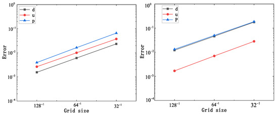
Figure 2. The trend of the errors with the grid size: Scheme I (left); Scheme II (right).

4.2. Annihilation and Stable Defects

The numerical example was associated with the phenomenon of the annihilation of singularities. We considered many numerical experiences consisting of the motions of the singularity. We simulated evolutions of the director vector $\mathbf{d}$ field over time under certain conditions. The motion of defect points in liquid crystals can be simulated via the long-time behavior of the harmonic map flow. Moreover, the disappearance of singularity is affected by the direction. Finally, the defects would move toward a steady state. We simulated the dynamic evolution of singularities until the simulation reached the steady state. For the different initial values of $\mathbf{d}$, we give the annihilation phenomena of the singularities. A comparison of the annihilation for different initial directors in two schemes is presented. We considered the computational domain in the unit circle $\mathrm{\Omega }=(x,y):x^2+y^2<1$, and the following parameters were chosen: $\tau =0.05$, $h=\frac{1}{50}$, $\gamma =0.18,\lambda =0.01,\eta =0.1$, and $ϵ=0.05$.

For Scheme I, we chose the initial conditions as follows:

$$\begin{array}{c}\hfill \mathbf{u}=\mathbf{0},p=0,\mathbf{d}=(sin(\pi {(x^2+y^2)}^2),cos(\pi {(x^2+y^2)}^2)).\end{array}$$

The evolutions of the director field $\mathbf{d}$ and the velocity field $\mathbf{u}$ at different times are displayed in Figure 3 and Figure 4, where $T=3$ is the stoping time of the iteration.

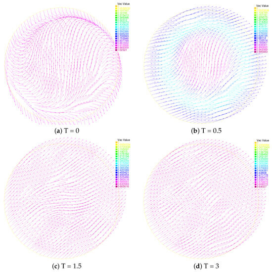
Figure 3. Evolution of the director fields of Scheme I: T = 0 (top left), T = 0.5 (top right), T = 1.5 (bottom left), T = 3 (bottom right).

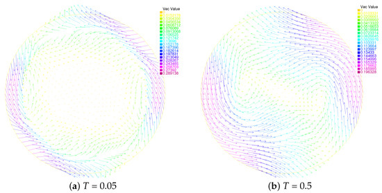
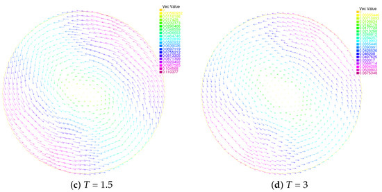
Figure 4. Evolution of the velocity fields of Scheme I: T = 0.05 (top left), T = 0.5 (top right), T = 1.5 (bottom left), T = 3 (bottom right).

For Scheme II, the initial conditions were taken as follows:

$$\begin{array}{c}\hfill \mathbf{u}=\mathbf{0},p=0,\mathbf{d}=(sin(2\pi (cosx-siny)),cos(2\pi (cosx-siny))).\end{array}$$

By changing the initial directors, we present the phenomenon of the annihilation of singularities. We also found a small difference in the molecule orientation near the boundary. Figure 5 and Figure 6 show the simulation results for the annihilation of singularities.

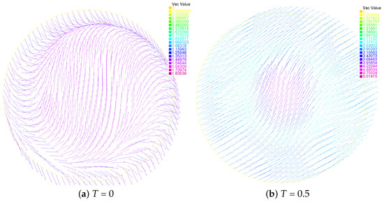
Figure 5. Evolution of the director fields of Scheme II: T = 0 (top left), T = 0.5 (top right), T = 1.5 (bottom left), T = 3 (bottom right).

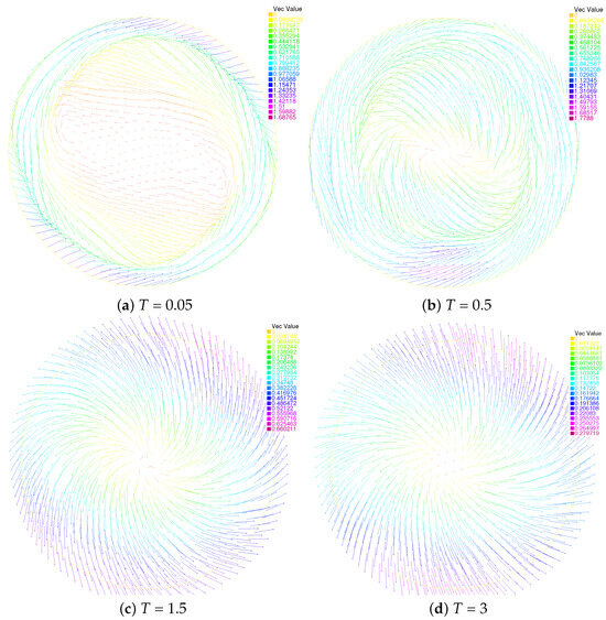
Figure 6. Evolution of the velocity fields of Scheme II: T = 0.05 (top left), T = 0.5 (top right), T = 1.5 (bottom left), T = 3 (bottom right).

‘Vec Value’ in Figure 3, Figure 4, Figure 5 and Figure 6 is the abbreviation of ‘Vector Value’. The arrows in the figure represent the directions of the molecules, and different colors represent different numerical sizes. In Figure 3, we plot the director field $\mathbf{d}$ at four different times: at $t=0$, where the singularities are swirled around with the flow; at $t=0.5$, where the singularities clearly keep on moving with the flow; after $t=1.5$, where the change trend starts moving in one direction. Figure 5 is the same. In Figure 4, we plot the velocity field $\mathbf{u}$ at four different times: at $t=0.05$, where the singularities are swirled around with the flow; at $t=0.5$, where the singularities keep on moving closer and closer to each other with the flow; at $t=1.5$, with the singularities just prior to annihilation; finally, at $t=3$, where the steady state is reached. Similarly, we find that the steady state begins to be reached roughly after $t=1.5$ in Figure 6.

4.3. The Dissipation of Energy

In this section, we describe the test of the energy decay for the proposed schemes. The discrete energy functional for Scheme I can be written as

$$E({\mathbf{u}}_h^{n+1},{\mathbf{d}}_h^{n+1})={\int }_{\mathrm{\Omega }}({\displaystyle \frac{1}{2}}\mid {\mathbf{u}}_h^{n+1}{\mid }^2+{\displaystyle \frac{\lambda }{2}}\mid \nabla {\mathbf{d}}_h^{n+1}{\mid }^2+{\displaystyle \frac{\lambda }{4{ϵ}^2}}{(\mid {\mathbf{d}}_h^{n+1}{\mid }^2-1)}^2)dx.$$

In the test, we considered a numerical experience consisting of the motion of two singularities. In order to simulate the time behavior of different energies interacting in the system, we defined the kinetic and elastic energies as

$$\begin{array}{c}\hfill E_{kin}=\frac{1}{2}{\parallel \mathbf{u}\parallel }^2,E_{ela}=\frac{\lambda }{2}{\parallel \nabla \mathbf{d}\parallel }^2+\frac{\lambda }{4{ϵ}^2}{\parallel {\mathbf{d}}^2-1\parallel }^2.\end{array}$$

Scheme I of the Ericksen–Leslie hydrodynamic model was computed in the domain $[-1,1]\times [-1,1]$, and the initial conditions were

$$\begin{array}{c}\hfill \mathbf{u}=\mathbf{0},p=0,{\mathbf{d}}_0=(\frac{\overline{\mathbf{d}}}{\sqrt{\mid \overline{\mathbf{d}}{\mid }^2+{ϵ}^2}}),\overline{\mathbf{d}}=(x^2+y^2-0.25,y).\end{array}$$

The evolution of the kinetic and elastic energies is depicted in Figure 7, Figure 8, Figure 9 and Figure 10. Here, Figure 7 and Figure 8 show the results of the kinetic energy and elastic energy in comparison with the different time steps. Similarly, it was found that the energies were acceptable for $E_{kin}$ and $E_{ela}$ in comparison with the variables $\gamma , \lambda , \eta$, and $ϵ$ in Figure 9 and Figure 10, respectively.

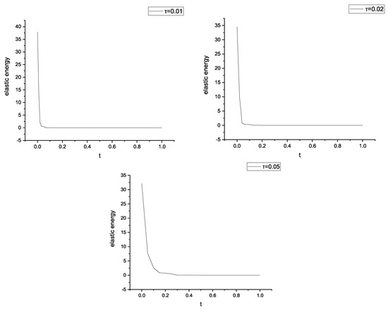
Figure 7. The different time steps of elastic energy.

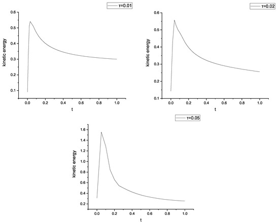
Figure 8. The different time steps of kinetic energy.

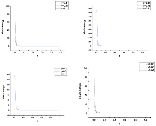
Figure 9. The different parameters of elastic energy.

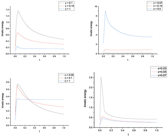
Figure 10. The different parameters of kinetic energy.

In Figure 7 and Figure 8, we also plot the condition parameters in terms of the time step $\tau$ for different values of $E_{kin}$ and $E_{ela}$. No matter how large or small, the elastic energy changed only a little. However, the degree of kinetic energy dissipation became more obvious with the increase in the time step.

It was obvious that the condition parameters of the matrix were not sensitive to $\gamma , \lambda , \eta ,$ and $ϵ$, as shown in Figure 9. The velocity was dissipated, and the elastic energy showed a slow decay.

Furthermore, we found that the kinetic energy reached its maximum level at the annihilation time in Figure 10. The results verified our expectations. Therefore, these numerical results were achieved as expected.

5. Conclusions

To study numerical approximations for the modified Ericksen–Leslie model, this study designed two different fully discrete finite element schemes. One was the numerical scheme of the second-order backward differentiation formula, and the other was the leap frog scheme. Their key idea was based on a novel convex splitting method, which was a unique way to skillfully deal with the nonlinear term. We not only rigorously proved the unconditional energy stability, but we also showed a detailed practical implementation for both schemes. A large number of numerical results showed that the order of convergence of the two schemes was of the second order in both time and space. Significantly, the numerical experiments also showed that the leap frog scheme was more computationally efficient than the backward differentiation formula.

References

- Rey, A.D.; Denn, M.M. Dynamical phenomena in liquid-crystalline materials. Annu. Rev. Fluid Mech. 2002, 34, 233–266. [Google Scholar] [CrossRef]
- Ericksen, J. Hydrostatic theory of liquid crystal. Arch. Ration. Mech. Anal. 1962, 9, 371–378. [Google Scholar] [CrossRef]
- Ericksen, J.L. Conservation laws for liquid crystals. J. Rheol. 1961, 5, 23–34. [Google Scholar] [CrossRef]
- Ericksen, J.L. Liquid Crystals with Variable Degree of Orientation. IMA Preprint Ser. 1989, 559. [Google Scholar] [CrossRef]
- Leslie, F.M. Some constitutive equations for liquid crystals. Arch. Ration. Mech. Anal. 1968, 28, 265–283. [Google Scholar] [CrossRef]
- Ball, J.M. Mathematics and liquid crystals. Mol. Cryst. Liq. Cryst. 2017, 647, 1–27. [Google Scholar] [CrossRef]
- Climent-Ezquerra, B.; Guillen-González, F. Convergence to equilibrium for smectic-A liquid crystals in domains without constraints for the viscosity. Nonlinear Anal. 2014, 102, 208–219. [Google Scholar] [CrossRef]
- Liu, C.; Walkington, N.J. Approximation of liquid crystal flows. SIAM J. Numer. Anal. 2000, 37, 725–741. [Google Scholar] [CrossRef]
- Chen, C.J.; Yang, X.F. Fully-decoupled, energy stable second-order time-accurate and finite element numerical scheme of the binary immiscible Nematic-Newtonian model. Comput. Methods Appl. Mech. Eng. 2022, 395, 114963. [Google Scholar] [CrossRef]
- Zhang, X.; Wang, D.X.; Zhang, J.W.; Jia, H.E. Fully decoupled linear BDF2 scheme for the penalty incompressible Ericksen-Leslie equations. Math. Comput. Simulat. 2023, 212, 249–266. [Google Scholar] [CrossRef]
- Lin, F.; Liu, C. Nonparabolic dissipative systems modeling the flow of liquid crystals. Commun. Pure Appl. Math. 1995, 48, 501–537. [Google Scholar] [CrossRef]
- Ping, L.; Liu, C. Simulations of singularity dynamics in liquid crystal flows: A C0 finite element approach. J. Comput. Phys. 2006, 215, 348–362. [Google Scholar]
- Guillen-Gonzalez, F.M.; Gutirrez-Santacreu, J.V. A linear mixed finite element scheme for a nematic EricksenCLeslie liquid crystal model. ESAIM Math. Model. Numer. Anal. 2013, 47, 1433–1464. [Google Scholar] [CrossRef]
- Girault, V.; Guillen-Gonzalez, F. Mixed formulation, approximation and decoupling algorithm for a penalized nematic liquid crystals model. Math. Comput. 2011, 80, 781–819. [Google Scholar] [CrossRef]
- Badia, S.; Guilln-Gonzlez, F.; Gutirrez-Santacreu, J.V. Finite element approximation of nematic liquid crystal flows using a saddle-point structure. J. Comput. Phys. 2011, 230, 1686–1706. [Google Scholar] [CrossRef]
- Bao, X.; Chen, R.; Zhang, H. Constraint-preserving energy-stable scheme for the 2D simplified Ericksen-Leslie system. J. Comput. Math. 2021, 39, 1. [Google Scholar] [CrossRef]
- Wang, D.; Miao, N.; Liu, J. A second-order numerical scheme for the Ericksen-Leslie equation. AIMS Math. 2022, 7, 15834–15853. [Google Scholar] [CrossRef]
- Cheng, K.; Wang, C.; Wise, S.M. An energy stable finite difference scheme for the Ericksen–Leslie system with penalty function and its optimal rate convergence analysis. Commun. Math. Sci. 2023, 21, 1135–1169. [Google Scholar] [CrossRef]
- Wang, D.; Liu, F.; Jia, H.; Zhang, J. Error estimates of a sphere-constraint-preserving numerical scheme for Ericksen-Leslie system with variable density. Discret. Contin. Dyn. Syst.-B 2023, 28, 5814–5838. [Google Scholar] [CrossRef]
- Miao, N.; Wang, D.; Zhang, H.; Liu, J. A second-order BDF convex splitting numerical scheme for the ericksen-leslie equation. Numer. Algorithms 2023, 94, 293–314. [Google Scholar] [CrossRef]
- Ren, Y.; Liu, D. Pressure correction projection finite element method for the 2D/3D time-dependent thermomicropolar fluid problem. Comput. Math. Appl. 2023, 136, 136–150. [Google Scholar] [CrossRef]
- Wang, S.; Zhu, M.; Cao, H.; Xie, X.; Li, B.; Guo, M.; Li, H.; Xu, Z.; Tian, J.; Ma, D. Contact Pressure Distribution and Pressure Correction Methods of Bolted Joints under Mixed-Mode Loading. Coatings 2022, 12, 1516. [Google Scholar] [CrossRef]
- Yang, X.F. Linear, first and second-order, unconditionally energy stable numerical schemes for the phase field model of homopolymer blends. J. Comput. Phys. 2016, 327, 294–316. [Google Scholar] [CrossRef]
- Shen, J.; Xu, J.; Yang, J. The scalar auxiliary variable (SAV) approach for gradient flows. J. Comput. Phys. 2018, 353, 407–416. [Google Scholar] [CrossRef]
- Shen, J.; Xu, J.; Yang, J. A new class of efficient and robust energy stable schemes for gradient flows. SIAM Rev. 2019, 61, 474–506. [Google Scholar] [CrossRef]
- Guilln-Gonzlez, F.; Tierra, G. On linear schemes for a Cahn Hilliard diffuse interface model. J. Comput. Phys. 2013, 234, 140–171. [Google Scholar] [CrossRef]
- Xu, X.; Van Zwiete, G.J.; van der Zee, K.G. Stabilized second-order convex splitting schemes for cahn-hilliard models with application to diffuse-interface tumor-growth models. Int. J. Numer. Methods Biomed. Eng. 2014, 30, 180–203. [Google Scholar]
- Shen, J.; Wang, C.; Wang, S.; Wang, X. Second-order convex splitting schemes for gradient flows with ehrlich-schwoebel type energy: Application to thin film epitaxy. SIAM J. Numer. Anal. 2012, 50, 105–125. [Google Scholar] [CrossRef]
- Elliott, C.M.; Stuart, A.M. The global dynamics of discrete semilinear parabolic equations. SIAM J. Numer. Anal. 1993, 30, 1622–1663. [Google Scholar] [CrossRef]
- Eyre, D.J. Unconditionally gradient stable time marching the Cahn-Hilliard equation. MRS Online Proc. Libr. (OPL) 1998, 529, 39–46. [Google Scholar] [CrossRef]
- Chandrasekhar, S. Liquid Crystals; Cambridge University Press: Cambridge, UK, 1992. [Google Scholar]
- de Gennes, P.G. The Physics of Liquid Crystals; Oxford University Press: London, UK, 1974. [Google Scholar]
- Ezquerra, M.B.C.; González, F.M.G.; Medar, M.A.R. Reproductivity for a nematic liquid crystal model. Z. FüR Angew. Math. Und Phys. Zamp 2006, 57, 984–998. [Google Scholar] [CrossRef][Green Version]
- Hecht, F.; Pironneau, O.; Ohtsuka, K. FreeFEM++. 2010. Available online: http://www.freefem.org/ff++/ (accessed on 16 February 2024).
Disclaimer/Publisher’s Note: The statements, opinions and data contained in all publications are solely those of the individual author(s) and contributor(s) and not of MDPI and/or the editor(s). MDPI and/or the editor(s) disclaim responsibility for any injury to people or property resulting from any ideas, methods, instructions or products referred to in the content. |
© 2024 by the authors. Licensee MDPI, Basel, Switzerland. This article is an open access article distributed under the terms and conditions of the Creative Commons Attribution (CC BY) license (https://creativecommons.org/licenses/by/4.0/).