KDTM: Multi-Stage Knowledge Distillation Transfer Model for Long-Tailed DGA Detection

Abstract

As the most commonly used attack strategy by Botnets, the Domain Generation Algorithm (DGA) has strong invisibility and variability. Using deep learning models to detect different families of DGA domain names can improve the network defense ability against hackers. However, this task faces an extremely imbalanced sample size among different DGA categories, which leads to low classification accuracy for small sample categories and even classification failure for some categories. To address this issue, we introduce the long-tailed concept and augment the data of small sample categories by transferring pre-trained knowledge. Firstly, we propose the Data Balanced Review Method (DBRM) to reduce the sample size difference between the categories, thus a relatively balanced dataset for transfer learning is generated. Secondly, we propose the Knowledge Transfer Model (KTM) to enhance the knowledge of the small sample categories. KTM uses a multi-stage transfer to transfer weights from the big sample categories to the small sample categories. Furthermore, we propose the Knowledge Distillation Transfer Model (KDTM) to relieve the catastrophic forgetting problem caused by transfer learning, which adds knowledge distillation loss based on the KTM. The experimental results show that KDTM can significantly improve the classification performance of all categories, especially the small sample categories. It can achieve a state-of-the-art macro average F1 score of 84.5%. The robustness of the KDTM model is verified using three DGA datasets that follow the Pareto distributions.

1. Introduction

The Internet has brought great convenience to people but it has also brought hidden dangers of network security while facilitating our lives. Botnet [1,2] attacks are one of the most common and destructive threats [3]. They are large-scale network attacks carried out by remotely controlled devices infected by malware. The botnet attack controls the infected hosts through the command and control (C&C) server [4] to launch DDoS attacks [5], send spam [6], generate false Internet traffic [7], and commit many other crimes and malicious acts. To bypass the detection of security devices, the production process of attackers is becoming more and more complex. To establish and maintain communication with the C&C server, attackers integrate the Domain Generation Algorithm (DGA) into the system to dynamically and randomly generate the domain names. This can increase the robustness of the botnet and the persistent control of the infected hosts. Therefore, if DGA domain names can be accurately detected, botnet control can be avoided. In the initial stage, the network security field uses the DGA domain names collected by information security intelligence to generate a blacklist [8]. Malicious domain names [9] are determined by checking against the blacklist, but the randomness and variability of DGA make it difficult to update the blacklist. Therefore, a scheme of using machine learning to detect DGA domain names was derived [10].

Traditional approaches mainly use feature extraction methods based on machine learning. They follow the process as below: statistical feature detection of domain name characters [10], Domain Name Server (DNS) traffic information detection [11], and traditional machine learning models to detect DGA domain names [12]. However, manual feature extraction is time-consuming and some hidden features are easy to ignore. Then came deep learning methods to detect DGA domain names, and additional conditions were considered for the deep learning methods to improve the detection ability [13]. In Section 2, we summarize the related work of deep learning on DGA detection. It can be seen that imbalanced sample sizes between categories can affect the overall detection results. However, the categories that can not be detected in network security are more dangerous. Therefore, to more accurately detect DGA categories with fewer samples, we introduced the long-tailed concept in the DGA detection problem in this paper. The DGA dataset follows the Pareto distribution. It greatly affects the classification ability of deep models. The classification results usually tend to the categories that contain large amounts of data, while the tail categories that contain small amounts of data have low accuracy. Or, even worse, to reduce the impact of long-tailed problems on deep network models, tail categories were cut off in previous DGA studies [14,15,16], leading to an incomplete DGA classification.

Although the long-tailed DGA problem was ignored in the literature, there are optimization methods for long-tailed problems in other fields. From the data perspective, the solutions mainly use resampling to balance the data volume between categories, but this causes over-fitting and losses of information [17]. From an algorithm perspective, the solutions mainly adjust the hyperparameters to balance the weights of the categories or adjust some training strategies to balance the impact of the categories. For example, the head categories transfer the knowledge to the tail categories [18]. However, some head knowledge may be forgotten during the transfer process, resulting in decreased accuracy of head categories. Knowledge distillation [19] can alleviate the catastrophic forgetting problem caused by transfer learning. Inspired by it, we propose a multi-stage Knowledge Distillation Transfer Model (KDTM) for long-tailed DGA detection. We divide the training task into multiple stages. Then, we use the Data Balanced Review Method (DBRM) to fill in the data for each stage to balance the category data at each stage. Finally, we apply multi-stage transfer weights with knowledge distillation to transfer the knowledge from the previous stage to the subsequent stage sequentially. We expect that the tail categories with insufficient knowledge can learn more from the head categories so that the overall classification accuracy can be improved, especially for the tail categories. The main contributions of this paper are as follows:

• We propose DBRM, which is a sampling method to transform long-tailed distribution data into a relatively balanced dataset. This method is used during the transfer learning phase to reduce the gap between the head and tail categories.
• We propose the Knowledge Transfer Model (KTM), which divides weight transfer into multi-stages and gradually transfers head category knowledge to tail categories to improve the classification performance of tail categories. The experimental results show that when all categories of data are equally divided into two stages, KTM has the best performance, with an overall performance of 79%.
• We propose KDTM, which applies knowledge distillation to compensate for the forgetting of head categories with large sample sizes during the transfer of the KTM. Further, it improves the detection accuracy of categories with small sample sizes. The experimental results show that the overall performance of all categories can reach 84.5%, and the accuracy of the tail categories has been improved by 12%.

The remaining chapters of this paper are briefly introduced as follows: Section 2 introduces recently related work for long-tailed problems and DGA detection methods. Section 3 defines the long-tailed DGA detection problem and our framework for resolving the problem. Section 4 introduces the dataset, ablation study, and experimental results. Section 5 concludes with the conclusions.

2. Related Work

2.1. DGA Detection

Botnets use DNS services to hide their C&C server [20]. The communication between the C&C server and the infected host runs the same set of DGA to generate the same list of alternative domain names. The infected host regularly connects and receives commands from the C&C server and the hackers control the infected host by sending the commands to the C&C server. At the initial stage of network security, a blocklist database is established to determine whether a domain name is malicious [8]. However, DGA can generate hundreds and thousands of domain names shortly, which makes it difficult to maintain and update the blacklist and it is difficult to detect unknown DGA domain names using an out-of-date blacklist.

Therefore, it is more convenient and effective to use machine learning methods to detect DGA domain names [21,22,23]. Traditional DGA domain name detection is mainly based on feature extraction and machine learning. It classifies the DGA domain names by detecting the difference in character distribution between the legal domain names and the DGA domain names. Davuth in [10] made the bigram of domain names as a feature, filtered the bigrams with low frequency through the method of artificial threshold and used the Support Vector Machine (SVM) classifier to detect random domain names. Bilge [11] used DNS analysis to detect the domain of malicious activities and described the different attributes of DNS names and the way to query them by extracting 15 features from the DNS traffic.

Then comes deep learning methods for DGA detection with the advantage of reducing the cost of manual feature extraction. Recurrent Neural Network (RNN) [24] is applied in various natural language tasks due to its ability to capture meaningful temporal relationships between sequences. However, RNN is prone to the gradient disappearance problem in the long-chain operation and does not have the ability to learn long-term information dependence. Woodbridge [14] used Long Short-Term Memory (LSTM) networks to achieve the real-time detection of DGA domain names without the context information and manually created features. LSTM adds state information on the basis of RNN to enable it to learn long-term information dependence. It is good at text and speech processing in the long-term learning mode. In order to compare the advantages of deep learning methods, Tong [25] proposed an LSTM network with an attention layer method for binary classification and multi-classification of DGA families. Yu [15] used the feature-based random forest model, which is an effective traditional machine learning method. However, compared with the LSTM network and Convolutional Neural Network (CNN), this method does not perform well on some specific DGA categories. Chen [16] proposed an LSTM model combined with an attention mechanism. This model focused on the more important substrings in the domain to improve the representation of the domain and achieve better performance, especially for long domain names. A model combining BiLSTM and CNN with an attention mechanism was proposed in [26], which effectively improved the detection accuracy of DGA categories. However, the classification results of the categories with a small amount of data were not ideal. The reason is that the imbalance of DGA data leads to large classification errors for those tail categories. In this condition, when dealing with the DGA data, we found that many studies chose to cut off the tail categories so that those DGA categories could not be classified. We have summarized the related work in the past few years in Table 1. We use the number of categories as the standard to classify DGA families into Many, Medium, and Few, which can provide a clearer view of the distribution of data volume within the dataset. In the traditional deep learning model [27,28,29], without considering the difference in sample size between categories. The higher the degree of imbalance in the dataset, the greater the impact on the overall performance of DGA detection (where we use the Macro average value to evaluate). In subsequent research, ref. [25,26,30,31,32,33] chose to cut out a few sample categories to improve the detection accuracy of other categories. But in network security, the uncommon DGA categories with few samples are the ones that we should be cautious about because hackers use uncommon DGA to increase the probability of successful intrusion. Therefore, we need to consider the long-tailed problem of DGA and use methods to address it to improve the overall performance of detection.

Table 1. Related work of detecting Domain Generation Algorithm (DGA) domain names based on deep models. We divided DGA Families into Many, Medium, and Few categories based on the sample size of the categories for analysis. The sample size of Many categories is greater than 10,000, while the sample size of Few categories is less than 1000. Other categories are classified into Medium. The imbalance factor [34] is one of the indicators used to evaluate whether a dataset is balanced. The Macro average F1 score [35] is used to evaluate the model detection effect.

Method	Year	Datasets	DGA Families			Family Sample Range (Max–Min)	Imbalance Factor	Macro Average F1 score
			Many	Medium	Few
LSTM [14]	2016	Bambenek Consulting (DGA) Alexa(whitelist)	30			81,281–9	9031	0.541
RNN [27]	2017	Bambenek Consulting and DGArchive (DGA) Alexa (whitelist)	42	11	10	434,215–52	8157	0.66
SVM and LSTM-based models [28]	2017	Bambenek Consulting (DGA) Alexa (whitelist)	1	9	27	42,166–25	1686	0.2695
LSTM.MI [36]	2018	Bambenek Consulting (DGA) Alexa (whitelist)	1	9	27	42,166–25	1686	0.5671
CNN [37]	2019	DGArchive (DGA) Alexa (whitelist)	73			-	-	0.6123
ATT_CNN + BiLSTM [30]	2019	360netlab and Bambenek Consulting (DGA) Alexa (whitelist)	13	3	3	25,000–210	119	0.81
ATT_CNN + BiLSTM [26]	2020	360netlab Alexa (whitelist)	13	8	3	26,520–210	126	0.83
CNN_LSTM [38]	2020	OSINT Feeds (DGA) Alexa and OpenDNS (whitelist)	-	-	-	-	-	-
B-LSTM/B-RNN/B-GRU [29]	2021	Bambenek Consulting (DGA) Alexa (whitelist)	1	9	27	42,166–25	1686	0.47
ATT_BiLSTM [32]	2021	Bambenek Consulting (DGA) Alexa (whitelist)	11	9	0	439,223–2000	219	0.8369
LA_Bin07/LA_Mul07 [25]	2022	UMUDGA (DGA) Alexa (whitelist)	50	0	0	500,000–10,000	50	-
Extended Character Feature in BiLSTM [31]	2022	360netlab (DGA) Alexa (whitelist)	10	16	13	498,620–193	2583	0.7514
MHSA-RCNN-SABILSTM [33]	2022	360netlab and Bambenek Consulting (DGA) Alexa (whitelist)	11	9	0	439,223–2000	219	0.8397
PEPC [39]	2022	DGArchive, Bambenek Consulting and 360netlab (DGA) Alexa (whitelist)	20			-	-	0.8046
TLM [40]	2023	360netlab (DGA) Alexa (whitelist)	10	9	12	452,428–132	3427	0.766

2.2. Long-Tailed Problem

At present, the long-tailed problem in DGA detection has not received widespread attention from scholars, but there have been many studies on the long-tailed problem in other application scenarios. The traditional approach to solve the long-tailed problem is resampling consisting of over-sampling for the classes with few samples [41] and sub-sampling [42] for classes with many samples. However, over-sampling tends to overfit the minor class, it can not learn the robust and general abilities, and it often performs worse on imbalanced data. Under-sampling causes serious information loss for the class with many samples resulting in under-fitting. In DGA data with multiple categories and large data volume differences between categories, the direct use of resampling is not applicable.

During the training, re-weighting aims to re-balance the classes by altering the loss values for the distinct classes. The most intuitive way for loss re-weighting is to use the label frequencies of training samples directly, known as weighted softmax loss. In addition to loss re-weighting, the balanced softmax in [43] used the label frequencies to alter the model detection during the training, allowing the past information to mitigate the bias of the data imbalance. Therefore, if re-weighting is used in DGA detection, it sets different weights for different categories based on losses and greater weights for the few-shot category. However, it requires excessive human intervention to manually decide the weights.

Transfer learning [44,45,46,47,48] aims to improve the training of the model on a target domain by transferring information from a source domain (e.g., datasets, tasks, or classes). Tail data can be seen as samples to fine-tune downstream tasks using a large-scale model [49]. Head-to-tail knowledge transfer [18,50] aims to improve model performance on the tail categories by transferring knowledge from the head categories. There are two main types of head-to-tail knowledge transfer: feature transfer and weight transfer. Feature Transfer Learning (FTL) [18] uses head-class and intra-class variance to direct the feature augmentation for the tail-class samples, resulting in more intra-class variance in tail-class features and improving the tail-class performance. GIST was [51] proposed to transfer the weights of the classifier from the head to the tail. The head categories with most of the weight parameters of the classifier can be used to enhance the classifier weights of the tail categories. However, if there are many tail categories, not all tail categories can learn the knowledge of the head categories. At the same time, there are multiple categories in the DGA categories that have high similarities and are easily confusing. Therefore, it is necessary to divide categories into multiple stages, so that the weights can be gradually transferred to the tail categories. However, during the transfer process, it may cause catastrophic forgetting [52] for header categories knowledge.

2.3. Knowledge Distillation

Knowledge distillation uses a pre-trained teacher model to guide a student model [19,53]. Knowledge distillation for long-tailed learning has been the subject of several recent studies. To deal with the long-tailed instance segmentation, the Learning to Segment the Tail (LST) [54] method created a class-incremental learning technique, in which knowledge distillation was employed to combat catastrophic forgetting. The Learning From Multiple Experts (LFME) method [55] used the numerous subgroups datasets and then trained the multiple experts with the subsets. LFME used adaptive knowledge distillation with instance selection from easy to hard, which trained a unified student model based on these experts. Routing dIverse Distribution-aware Experts (RIDE) [56] presented a knowledge distillation approach by training a student network with fewer experts based on the multi-expert framework. Therefore, knowledge distillation can be used as an auxiliary method for transfer learning to alleviate catastrophic forgetting and can be applied to our problem.

3. Method

We have provided a detailed explanation of our method in this section. In Section 3.1, we define the DGA long-tailed problem. Section 3.2, Section 3.3, and Section 3.4, respectively, introduce the specific implementations of DBRM, KTM, and KDTM.

3.1. Long-Tailed DGA Detection Problem

DGA domain name categories $c\in \left\{1,2,\dots ,C\right\}$ from a long-tailed DGA dataset $D={\left\{(x_i,y_i)\right\}}_{i=1}^H$, where $x_i$ denotes an input of the $i-th$ sample and the $y_i$ denotes the corresponding category. We assume a training

$$f:arg\underset{\omega }{m}inL(D,\omega )$$

(1)

where $\omega$ denotes the model parameters. During model training, the model parameters are adjusted iteratively and accordingly, with the goal of minimizing the loss function L. In multiple classification problems, the difference in the sample size of different categories in D will make $\omega$ more biased toward categories with more samples. Therefore, the larger the sample size gap between categories, the easier for few-shot categories to be ignored. This will also affect the final training results of f. Therefore, the data imbalance of D is defined as a Pareto distribution.

The Pareto distribution [57] is named after Vilfredo Pareto. The Pareto principle is also known as the 80–20 rule. If X is a random variable with Pareto distribution, the probability that X is bigger than a number x, i.e., the tail function, is given by:

$$\overline{F}\left(x\right)=P_r(X>x)\left\{\begin{array}{cc}{\left(\frac{x_m}{x}\right)}^a& x\ge x_m\\ 1& x<x_m\end{array}\right.$$

(2)

The scale parameter $x_m$ (the minimal possible value of X) and the shape parameter $\alpha$, often known as the tail index, defines the Pareto distribution. $H:={\sum }_{c=1}^C{H}_c$ is defined as the total sample size of dataset D, and $H_c$ as the sample size of category c. $H_c$ is sorted in descending order so that $H_1\ge H_2\ge \cdots \ge H_C$. The imbalance factor [34] to measure the long-tailed distribution is defined below:

$$IF=\frac{max\left\{H_1,H_2,\dots ,H_C\right\}}{min\left\{H_1,H_2,\dots ,H_C\right\}}=\frac{H_1}{H_C}$$

(3)

However, it cannot reflect the overall characteristics of DGA datasets as the middle categories are not considered in $IF$. In this paper, we use $\alpha$ of $\overline{F}\left(x\right)$ to measure the long-tailed problem of DGA datasets. The larger the $\alpha$, the greater $IF$, the more imbalanced D, and the more significant the gap between $H_1$ and $H_C$. Therefore, for the detection of long-tailed datasets D, we want to detect more few-shot categories and improve the overall detection result of f by changing D to relatively balanced datasets, and modifying the training strategies of $\omega$ and L for knowledge enhancement in the few-shot categories. Algorithm 1 shows the specific implementation structure of our method. We divide the model into multiple stages for training, using DBRM to obtain a relatively balanced dataset in each stage, using KTM for knowledge transfer in each stage, and KDTM using the transferred ${\omega }_n$ and L to enhance knowledge.

Algorithm 1 Knowledge distillation transfer model

1: $N:$ denotes the number of stages 2: $K_N:$ denotes first category of stage N 3: $n:$ denotes current stage 4:   Input: ${\left\{D_c\right\}}_{c\in \left(0,K_N\right]}$                  ▹ Data pre-processing 5:   Output: ${\omega }_N$                 ▹ The final stage model parameters 6: ${\omega }_1⟵arg\underset{{\omega }_1}{m}in{L}_{CE}({\left\{D_c\right\}}_{c\in \left[K_1,K_2\right)},{\omega }_1)$           ▹ Base classes training 7: for$n=2$ to N do 8:   $D_n^{br}⟵$ DBRM$\left({\left\{D_c\right\}}_{c\in \left[K_1,K_{n+1}\right)}\right)$ 9:    ${\omega }_n⟵$ KTM$(D_n^{br},{\omega }_{n-1})$ 10:   ${\omega }_n⟵arg\underset{{\omega }_n}{m}in{L}_{KD}(D_n^{br},{\omega }_n)$ 11: end for 12: return${\omega }_n$

3.2. DBRM

We divide training into multiple stages, but there is also a significant difference in sample size between each stage. We use an under-sampling strategy to obtain a relatively balanced dataset at each transfer stage to narrow the sample size gap between stages. For example, if we split the training data into two stages: the first stage is from category 0 to category 15 (containing 90% of the data in the DGA dataset) and the second stage is the remaining classes. When training for the second stage, if all the data used in the first stage are inputted into the second stage, the data volume in the second stage is imbalanced.

We assume that the latter stage does not inherit the data from the previous stage. In this case, the detector may forget the previous stage category. This results in the deep model being unable to detect all categories. To solve this problem, we define the DBRM strategy as below:

(1)

$K\in R^d$ is the step size for each stage category, and for stage N, ${\left\{K_n\right\}}_{n=1,2,\dots ,N}$ is the step size of stage n. Categories $[K_1,K_2)$ are termed as base categories and $K_1=1$. For stage n, categories $[K_1,K_n)$ are the old categories, $[K_n,K_{n+1})$ are the new categories, and $[K_{n+1},K_N]$ are the future categories. Datasets $D_n^{new}={\left\{D_c\right\}}_{c\in \left[K_n,K_{n+1}\right)}$ contain new categories and $D_n^{old}={\left\{D_c\right\}}_{c\in \left[K_1,K_n\right)}$ contain old categories.

(2)

Obtain the review datasets $D_n^{sample}$: For each category in $[K_1,K_n)$, randomly sample $H_{K_n}$ samples from $D_n^{old}$.

(3)

By using the balanced datasets $D_n^{sample}$ of the old categories, we replay $D_n^{sample}$ into each stage $D_n^{old}$ to obtain a relatively balanced datasets $D_n^{br}=D_n^{sample}\cup D_n^{new}$ as the training datasets.

In addition, we have concretely presented DBRM in Figure 1 for better understanding. To narrow the gap between large sample size categories and small sample size categories, we use an under-sampling strategy in large sample size categories for each transfer stage based on small sample size categories. This can maintain a relatively balanced sample size during the migration phase and, to a greater extent, avoid the model’s neglect of small sample size categories. Figure 1 shows that DBRM reduces the amount of data for large sample categories in the base data through an under-sampling strategy. In the final stage N, it can be seen that the amount of data for large sample categories is relatively balanced with that for small sample categories.

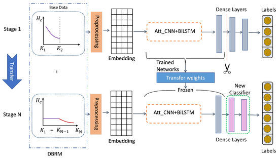
Figure 1. The architecture of the Knowledge Transfer Model (KTM). The purple and red lines indicate the distribution trend of sample size for each category.

3.3. KTM

3.3.1. Base Data

Dataset D is obtained by sorting all categories in descending order according to the number of samples. Multi-stage learning divides D into multiple non-overlapping sub-datasets $D_n$, $n=1,2,\cdots ,N$. $D_1$ is used to train the base teacher model and includes the categories with relatively large amounts of data in dataset D.

3.3.2. Preprocessing

As shown in Table 2, there are many types of characters in the DGA dataset. we replace the characters in the domain name with numbers. We map alphabetic characters (a–z), numbers (0–9), and special characters (., _, -) to integers 0 to 39; DGA domain names have different lengths. Since the maximum length of DGA domain names is 73, we use the filling to make all the domain names have equal lengths so that domain names are ready to be inputted into the deep learning model.

Table 2. The detailed Domain Generation Algorithm (DGA) dataset.

DGA Family	Sample	DGA Family	Sample
Alexa (whitelist)	google.com	qadars	9u78d6349qf8.top
banjori	bplbfordlinnetavox.com	locky	tcrgkleyeivrlix.work
emotet	fdfptbhnadweuudl.eu	dyre	g6a8ff179bf317e57b2b6665d3fdc47dc0.to
rovnix	oysyt45p4r3ul7sbdo.com	chinad	j0xx9q0a0p57o0up.cn
tinba	lkhhrrnldtoy.me.uk	cryptolocker	lmnlbvkcomdoh.biz
pykspa_v1	vjdibcn.cc	vawtrak	agifdocg.top
simda	welorav.info	pykspa_v2_fake	bvuhnesrlz.net
ramnit	hpgfsqdgbwvonp.com	dircrypt	extuhmqqtzwavpmfw.com
gameover	2okay8f2i4l7xadz0c1tt8rlw.biz	conficker	bxsujqbjrz.cc
ranbyus	eruvxfflddfkekhvd.su	matsnu	half-page-belt.com
virut	uiufzg.com	nymaim	yxcaitrv.in
murofet	wjspslenzlfruiy.com	fobber_v2	nqietkrebr.com
necurs	twxsbhjatburhmg.nf	fobber_v1	ayppvfettvcxdosqu.net
symmi	tucapefube.ddns.net	tempedreve	crpejdbfqf.net
shifu	updesxi.info	pykspa_v2_real	rjsxrxre.info
suppobox	alexandriawashington.net	padcrypt	cccdocfealldbnbf.tk

3.3.3. Embedding

Embedding is a method to convert discrete variables into continuous vectors of fixed length. It is very suitable for deep learning [58], using low-dimensional vectors to encode objects and preserve their meanings. Word embedding performs well in natural language processing, but because DGA domain names are generated using random characters and do not conform to the word rule in natural language, we use character-level embedding. In this paper, according to the padding size, the embedding input size is 73 and the output dimension is 32. To prevent over-fitting, we also use dropout and L2 regularization.

3.3.4. Att_BiLSTM + CNN Model

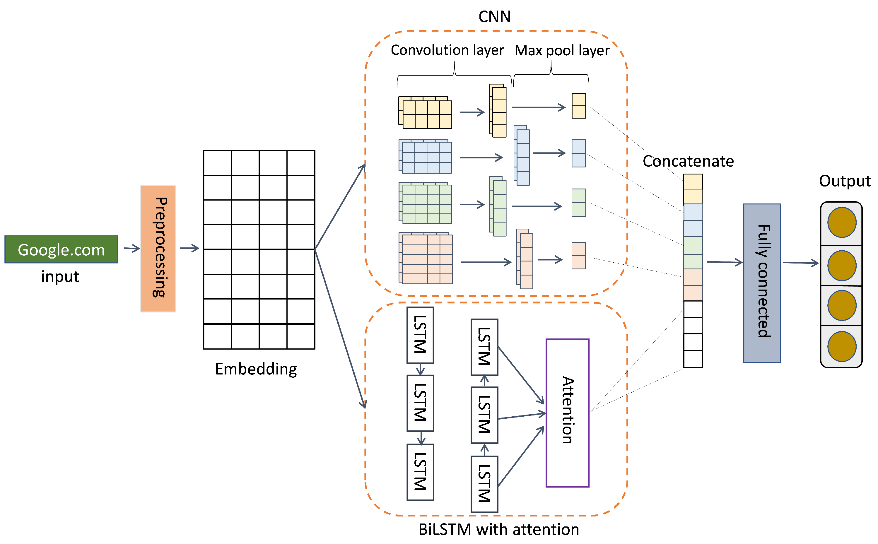
We use BiLSTM + CNN with an attention mechanism (ATT_BiLSTM + CNN) model [32] as the base teacher and comparison model, as shown in Figure 2.

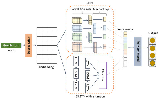
Figure 2. The architecture of the Att_CNN + BiLSTM model.

CNN [32] uses local area features to achieve target tasks. In the feature extraction stage, the convolution layer and pooling layer are repeatedly executed to automatically extract data features. Therefore, CNN can be used to learn the local sequence information of the DGA detection task and extract text features. BiLSTM [59] is a sequence processing model, and its name indicates that it is composed of bidirectional LSTM. It is commonly used in natural language tasks to model context information. By simulating human attention, an attention mechanism [60] is presented as a solution to the problem. In a nutshell, it is the process of swiftly separating high-value information from a large volume of data. Therefore, BiLSTM can learn global sequence information and understand the semantic information of the DGA data. We build the model and first input the pre-processing domain names into BiLSTM with attention and the CNN embedding layer, respectively. CNN includes four 1D convolution operations with different filter sizes from 2 to 5 and maximum pooling. We set the output size of the BiLSTM layer to be 256. To output each sequence, we set the theretun_sequence to True, add self-attention to BiLSTM to focus on important characters in the domain name, and then concatenate BiLSTM with attention and the CNN output layer. Finally, we obtain the DGA classification result through the full connection layer with ReLu as the activation function.

3.3.5. Transfer Weights

The specific segmentation of multiple stages is determined by the number of categories in the DGA datasets. We need to set the number of segmentation stages N, the total number of categories C of dataset D, and the number of categories in each stage $K=C/N$. If K is a non-integer, the stages except for the last stage contain rounded K categories, and the last stage contains the remaining categories. We use transfer learning to transfer the divided stage from the first stage to the last stage.

Transfer learning applies the knowledge learned from one task to other tasks. Transfer learning includes source domain $D_s$, $D_s=\left\{(x_{s_1},y_{s_1}),\dots ,(x_{s_i},y_{s_i})\right\}$ and target domain $D_T$, $D_T=\left\{(x_{T_1},y_{T_1}),\dots ,(x_{T_i},y_{T_i})\right\}$. $x_{s_i}$ is the data instance and $y_{s_i}$ is the corresponding class label, the inputs $x_{T_i}$ and $y_{T_i}$ are the corresponding outputs. So, transfer learning uses knowledge in the source domain $D_s$ and learning task $T_s$ to help improve the learning of target predictive function $f_T(·)$ in $D_T$.

As shown in Figure 1, starting from Stage 1, we use ${\left\{D_c\right\}}_{c\in \left[K_1,K_2\right)}$ as the input to train the base teacher model and save it as the basic pre-training model ${\omega }_1$. For Stage 2, we use $D_2^{br}$ as the model input. We obtain ${\omega }_2$ by loading and freezing the weight of ${\omega }_1$ trunk, and ${\omega }_2$ uses the weights of ${\omega }_1$ by changing the output layer. We gradually transfer data to obtain ${\left\{{\omega }_n\right\}}_{n=3,\dots ,N}$ using the same method. This multi-stage and gradual transfer approach can enable ${\omega }_n$ to learn from $\left\{{\omega }_{n-1}\right\}$ knowledge. Based on the above, ${\omega }_N$ can learn knowledge of all categories as the final model. We achieve weight transfer by freezing model parameters and cutting the last part of the dense layers to replace the new dense layers. This allows us to use the parameters of the frozen model and train only the latest dense layers. After completing the multi-stage weight transfer, the head categories with large sample data will transfer knowledge to the tail categories with small sample data. This can enhance the features of categories with small sample data.

3.4. KDTM

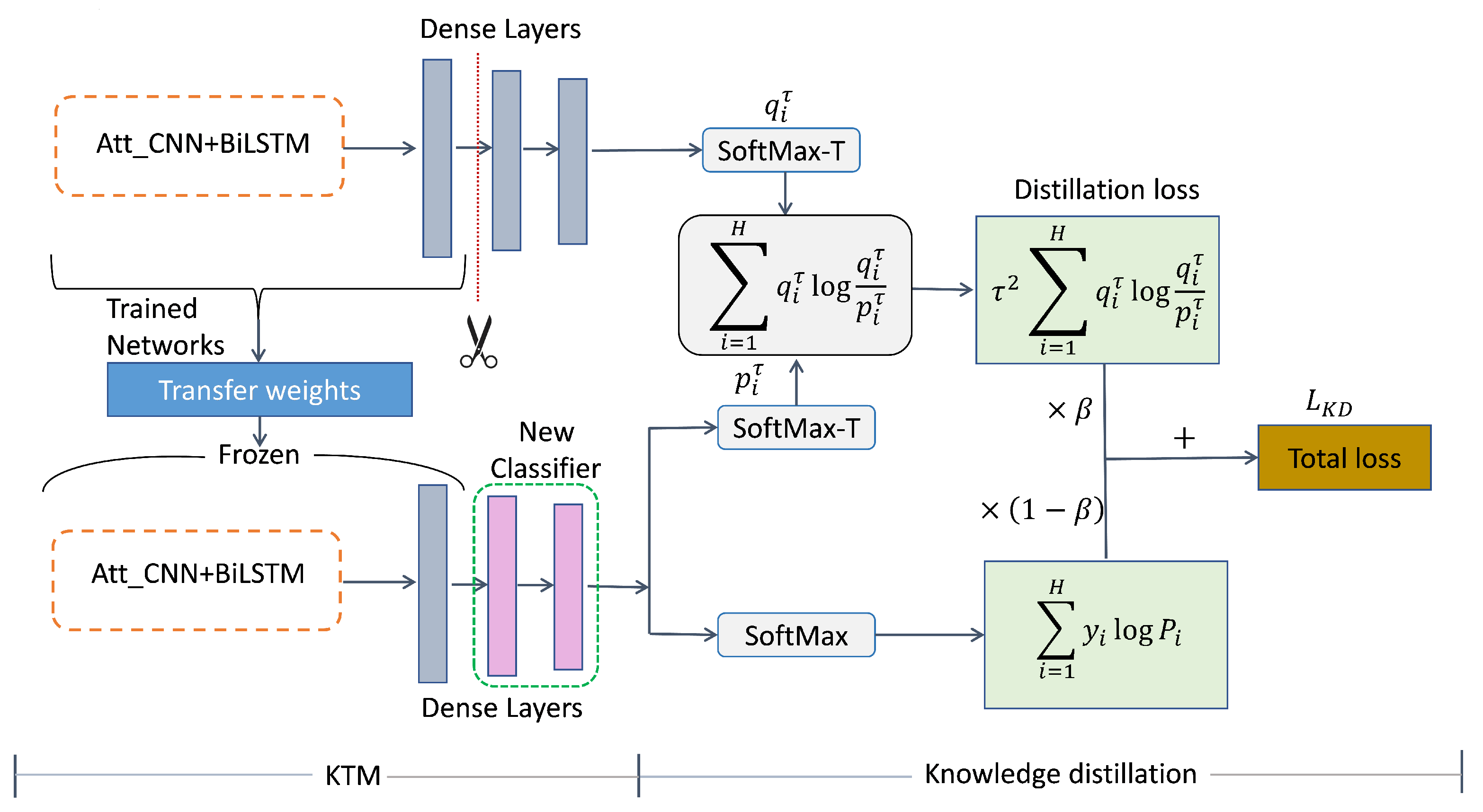
To further optimize KTM, we propose KDTM to alleviate ${\omega }_n$’s forgetting of ${\omega }_{n-1}$, which is the forgetting of head category knowledge. In Figure 3, we specifically demonstrate how KDTM uses knowledge distillation to retain the memory of ${\omega }_n$.

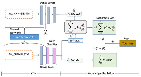
Figure 3. The architecture of the Knowledge Distillation Transfer Model (KDTM).

Knowledge Distillation

In our knowledge distillation, to alleviate the catastrophic forgetting of $\left\{{\omega }_{n-1}\right\}$ during the weights transfer process through knowledge distillation. ${\omega }_{n-1}$ is the exporter of the knowledge, and ${\omega }_{n-1}$ is the recipient of knowledge. Suppose that the ${\omega }_n$ predicts $p=\left(p_1,p_2,\dots ,p_H\right)\in R^H$ to obtain the Softmax function [61]:

$$p_i=\frac{exp\left(z_j\right)}{{\sum }_{k=1}^{H}exp\left(z_k\right)}$$

(4)

where $z_j$ is the ${\omega }_n$’s logits, H is the total number of labels. We add $\tau \in \left[1,20\right]$ to $p_i$ to smooth the output results and preserve the similarity information between ${\omega }_n$ and ${\omega }_{n-1}$. We denote the probability of each category, which is the inputting of the logits of ${\omega }_n$ to the Softmax-T function [19]:

$$p_i^{\tau }=\frac{exp\left(z_j/\tau \right)}{{\sum }_{k=1}^{H}exp\left(z_k/\tau \right)}$$

(5)

Similarly, $q_i^{\tau }$ denotes the probability of each category, which is the output of inputting the logits of ${\omega }_{n-1}$ into the Softmax-T function. Based on the above information, we have defined our distillation loss function as:

$$L_{KD}=(\beta +1)\sum _{i=1}^H{y}_{i}lo{g}_{p_i}+\beta {\tau }^2\sum _{i=1}^H{q}_i^{\tau }log\frac{q_i^{\tau }}{p_i^{\tau }}$$

(6)

where ${\sum }_{i=1}^H{q}_i^{\tau }log\frac{q_i^{\tau }}{p_i^{\tau }}$ denotes the Kullback–Leibler (KL) divergence loss [62] of $q_i^{\tau }$ and $p_i^{\tau }$ at the same temperature $\tau$, and can be expanded to:

$${\sum }_{i=1}^H{q}_i^{\tau }log\frac{q_i^{\tau }}{p_i^{\tau }}={\sum }_{i=1}^H{q}_i^{\tau }log{q}_i^{\tau }-q_i^{\tau }log{p}_i^{\tau }$$

(7)

which measures the distribution difference between ${\omega }_{n-1}$ and ${\omega }_n$. Similarly, ${\omega }_n$ can also receive knowledge of ${\omega }_{n-1}$.

The knowledge of ${\omega }_{n-1}$ can also have a certain error rate for ${\omega }_n$. Therefore, using ${\sum }_{i=1}^H{y}_{i}lo{g}_{p_i}$, which is the cross entropy [63] of ${\omega }_n$ including Softmax [64] $p_i$ can effectively reduce the possibility of errors being propagated to ${\omega }_n$. The weighted parameter $\beta \in [0,1]$ can balance the two parts of loss. To ensure the same contribution of the two parts of loss on the gradient amount, it is necessary to multiply the coefficient of ${\tau }^2$ before the second part of the loss.

Knowledge distillation is conducted based on transfer weights. Knowledge distillation has been proposed as a way to alleviate the catastrophic forgetting problem during the transfer weights process, but it can also add more knowledge of $\left\{{\omega }_{n-1}\right\}$ to ${\omega }_n$. For tail categories with small sample data, knowledge distillation means that more head category features will be transferred to the tail categories.

4. Experiments

We conducted extensive experiments to demonstrate how KDTM can improve the overall performance of DGA detection. Firstly, we conducted ablation experiments on the design in Section 4.3. Then, we benchmark our method on three long-tailed datasets with Pareto distributions, showing that it rivals or outperforms existing DGA detection methods.

4.1. Datasets

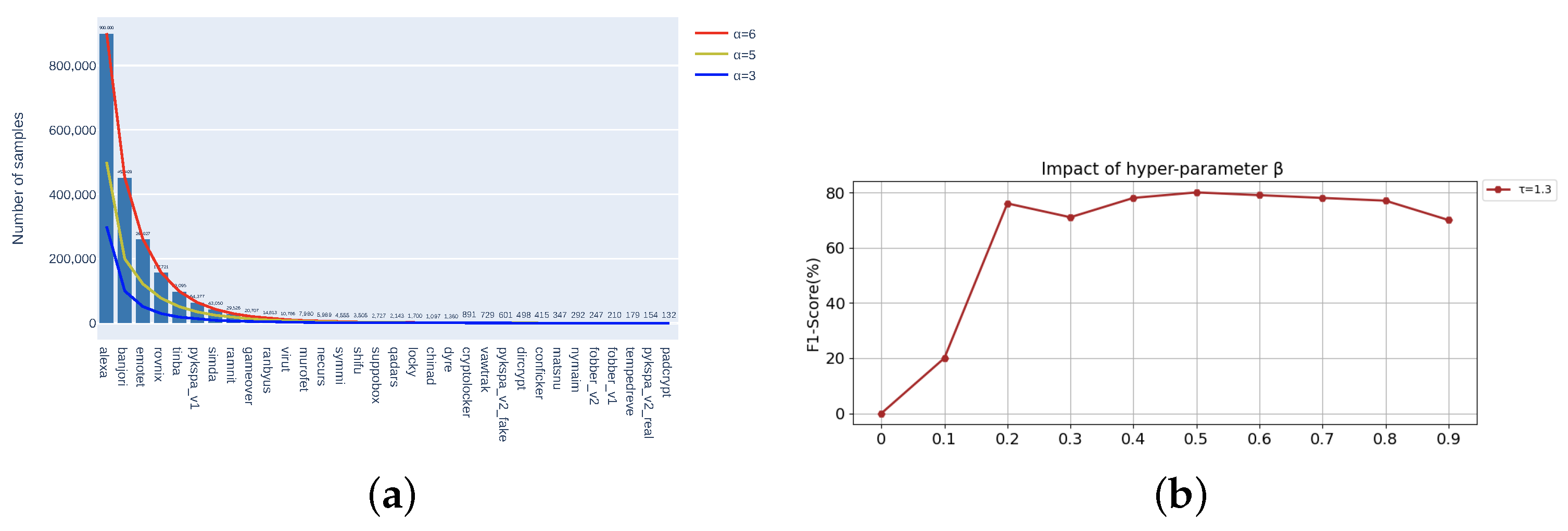
To better compare with other methods, we chose the dataset commonly used in deep learning DGA detection. Following [32], the long-tailed DGA dataset used in our experiments includes two broad categories of whitelist domain names and blacklist domain names. The whitelist domain names are obtained from the Alexa website (Alexa, The web information company (Seattle, WA, USA), http://www.alexa.com/ (accessed on 20 January 2023)), which ranks the domain names according to the number of users and visits. DGA domain names were obtained from a public dataset downloaded from the 360netlab (360netlab, https://data.netlab.360.com/dga/ or https://github.com/chrmor/DGA_domains_dataset (accessed on 20 January 2023) intelligence website including 31 DGA families. To verify the generalization of KDTM, we reshape the DGA datasets to follow Pareto distributions with $\alpha =3,5,6$ as shown in Figure 4a. When $\alpha =6$, the Pareto distribution basically matches the distribution of the original data. If $\alpha >6$, some tail categories will have too little data, and even some categories may not be able to obtain samples, so we choose power value $\alpha \le 6$. Overall, $\alpha =6$ contains 20.89281 M samples from 32 categories with the maximum of 9 M samples and the minimum of 132 samples, $\alpha =5$ contains 9.262 M samples with the maximum of 5 M samples and minimum of 169 samples, and $\alpha =3$ contains 5.5569 M samples with the maximum of 3 M samples and the minimum of 168 samples. From Figure 4a, it can be seen that for the difference in data volume between the head and tail, $\alpha =6>\alpha =5>\alpha =3$.

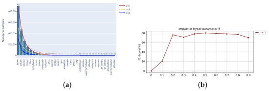
Figure 4. (a) The specific distribution of the datasets used to test model robustness . (b) The optimal value selection of hyper-parameter $\beta$ in $L_{KD}$.

4.2. Evaluation

We use $precision$ , $recall$, $F1$ score, and $macroaverageF1-Score$ [35] values as the evaluation indicators for model comparison.

$$precision=\frac{TP}{TP+FP}$$

(8)

$$recall=\frac{TP}{TP+FN}$$

(9)

$$F1=\frac{2\ast precision\ast recall}{precision+recall}$$

(10)

$$macroaverageF1-Score=\frac{sum(per\_class\_F1\_Score)}{count\left(class\right)}$$

(11)

where $TP$ is the true positive, $FP$ is the false positive, $FN$ is the false negative. The F1 score is the harmonic mean value of the precision rate and recall rate, which is equivalent to the comprehensive evaluation index of the precision rate and recall rate. Therefore, we mainly use the F1 score for comparison. The Macro average directly adds the evaluation indicators of different categories to calculate the average. By giving all categories the same weights, it treats each category equally, and better evaluates the overall effect of the model in the imbalanced multi-classification problem. We further reported the Macro average F1 score on three groups of categories, Many (category sample > 10,000), Medium (category sample 1000∼10,000), and Few (category sample < 1000), to comprehensively evaluate our model. We use the TensorFlow [65] toolbox to train our models. The models are trained with a batch size of 64 and the Adam [66] optimizer.

4.3. Ablation Study

4.3.1. Hyperparameter Tuning

$\beta$ and $\tau$ are the two hyperparameters in knowledge distillation. To prevent the information from being affected by the noise in the negative label, $\tau$ is set relatively low. Following [67], we use $\tau =1.3$. Figure 4b shows that the model can obtain the optimal result when $\beta =0.5$ and $\tau =1.3$. We can see that as a weighting parameter of two parts of loss in knowledge distillation, the F1 score value also increases with increased $\beta$. When $\beta =0.4$, F1 score tends to be stable, and the best result is when $\beta =0.5$.

4.3.2. Choosing N-Stage in KTM

We divide the total 32 categories of DGA datasets into multiple stages. In Table 3, to verify the impact of the number of stages on the classification performance, we choose the number of stages as follows: $N=2$, $N=3$, $N=4$ and $N=8$. The 2-stage, 4-stage, and 8-stage can be evenly distributed to each stage of $K=32/N$. The 3-stage is an example of uneven distribution, with $K=32/3$ categories in the first and second stages and $K=32/3$ categories in the third stage. The F1 scores of the Many, Medium, and Few categories of the 3-stage are all the lowest due to the uneven distribution of each stage category. The results of the 8-stage are also poor because the number of categories in each stage is too small and the transfer frequency is too high. According to the division rules of Many, Medium, and Few, Table 3 shows the results of transfer learning in multiple stages, we can see from the results that the 2-stage performs best in Many, Medium, Few, and All, and the 3-stage with non-average segmentation has the worst effect. With fewer stages and more even segmentation, the performance is better.

Table 3. Ablation studies comparing Knowledge Transfer Model (KTM) results across multiple stages through F1 scores, recall, and precision in the Many, Medium, and Few categories on Domain Generation Algorithm (DGA) long-tailed datasets of $\alpha =6$. The bolded values are the best in the same metrics and data blocks.

Metrics	N-Stage	Many	Medium	Few	All
F1	N = 2	0.941	0.930	0.558	0.792
	N = 3	0.686	0.660	0.245	0.497
	N = 4	0.870	0.875	0.580	0.766
	N = 8	0.761	0.678	0.349	0.561
Recall	N = 2	0.952	0.929	0.562	0.799
	N = 3	0.626	0.711	0.257	0.512
	N = 4	0.916	0.860	0.596	0.780
	N = 8	0.704	0.763	0.368	0.594
Precision	N = 2	0.922	0.935	0.652	0.825
	N = 3	0.798	0.782	0.353	0.627
	N = 4	0.853	0.900	0.594	0.769
	N = 8	0.818	0.677	0.421	0.630

4.3.3. Baseline and KTM

To demonstrate the effectiveness of KTM, we compare the baseline model without transfer learning with KTM. The baseline model is ATT_ BiLSTM + CNN, which is also the network architecture of KTM before using transfer weights. Figure 5a compares the baseline model and KTM per-class F1 score on DGA long-tailed datasets of $\alpha =6$. The blue part represents KTM, the gray part represents the baseline, and the darker part represents the overlapping part of the two values. From the results, it can be seen that the F1 score of KTM is much larger than that of the baseline model after the "Necaurs" category, which also proves that the combination of DBRM and weight transfer has a prominent contribution in categories with small sample sizes. In addition, categories with relatively large sample sizes also maintained relatively high accuracy. The overall effect of KTM is far superior to the baseline model.

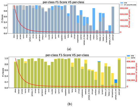
Figure 5. Ablation study comparing baseline model, Knowledge Transfer Model (KTM), and Knowledge Distillation Transfer Model (KDTM) per-class F1 score on Domain Generation Algorithm (DGA) long-tailed datasets of $\alpha =6$. (a) Comparison between KTM and baseline model (ATT_BiLSTM + CNN), where dark regions are the areas where their values overlap. (b) Comparison between KTM and KDTM.

4.3.4. Knowledge Distillation

Figure 5b compares the F1 scores of KTM and KDTM on the long-tailed dataset of α = 6. It shows the F1 score of KDTM (yellow) and KTM (blue) for all categories and their overlapping parts are shown in green. The red line is the distribution of the sample size of the categories, which follows the long-tailed distribution with $\alpha =6$. KDTM can greatly improve the accuracy of small sample categories while ensuring the accuracy of large sample categories and detect more DGA small sample categories. It can be seen that knowledge distillation has a memory ability for large sample categories of knowledge. This ability optimizes the forgetting of old knowledge when transferring weights and obtaining new knowledge to the small sample categories and it narrows the classification gap between the large sample categories and small sample categories in long-tailed data.

4.4. Comparison Methods and Results

4.4.1. Compared Methods

Considering the overall poor performance of deep learning in DGA detection in Table 1, we have chosen multiple methods that have been released in the past three years and have a relatively high Macro average F1 score, the BiLSTM with attention mechanism model (ATT_BiLSTM) [32] and CNN + BiLSTM model with attention mechanism (ATT_BiLSTM + CNN) [26]. The former two are the most recent and popular deep learning models for DGA detection problems.

4.4.2. Results

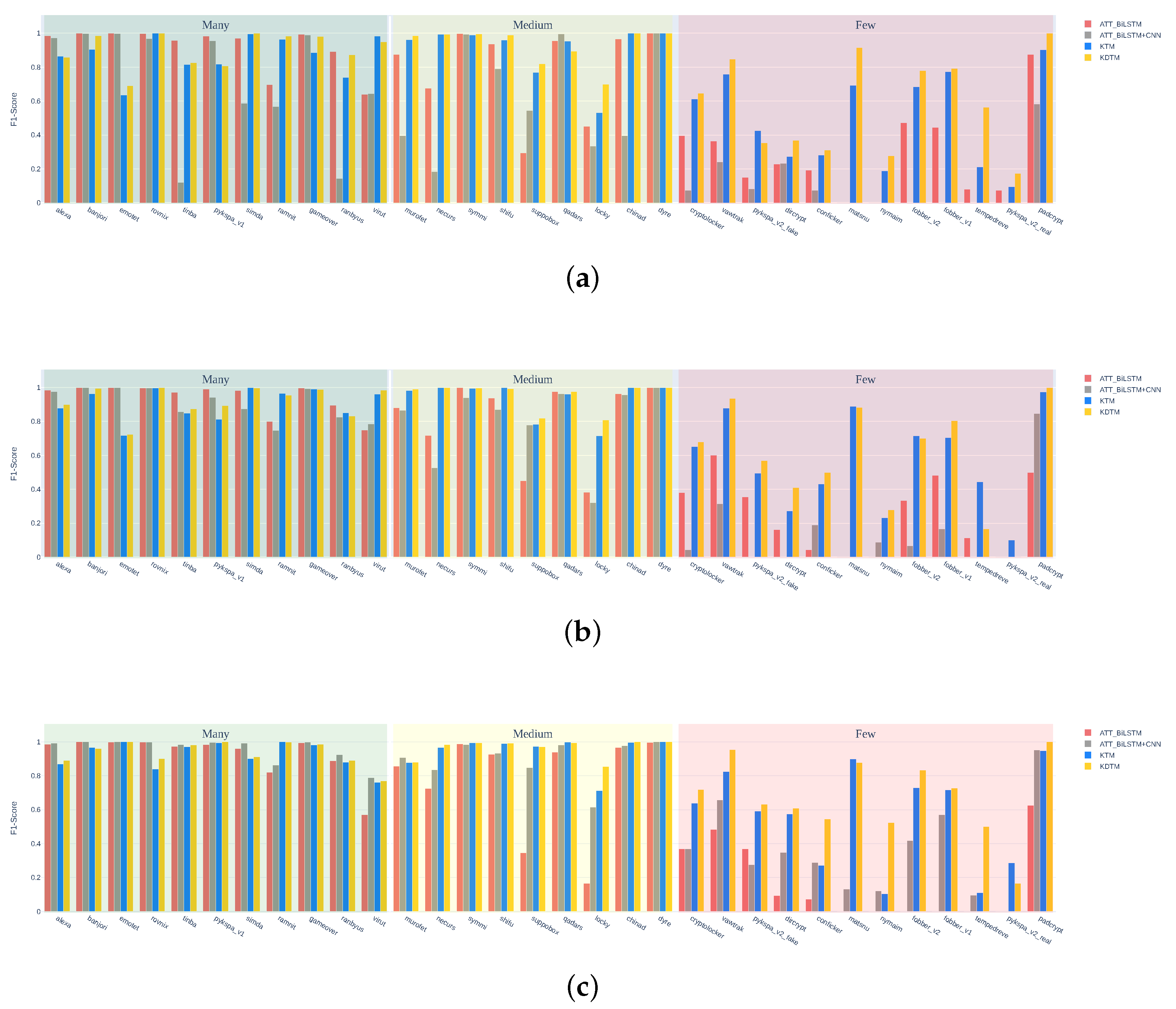
Figure 6 shows the detailed classification performance of each DGA category for all comparative models when using a DGA long-tailed distribution dataset with $\alpha =3$, $\alpha =5$, and $\alpha =6$. As expected, ATT_BiLSTM and ATT_BiLSTM + CNN have high accuracy in detecting categories belonging to Many, but for many categories belonging to Few, the detection accuracy is low, and some can not even be classified. We find that this situation is related to the dependence of traditional models on sample size. KTM knowledge transfer has a significant effect on categories belonging to Few. Compared to the two traditional models, categories from “dircrypt” to “pykspa_v2_real” can be basically classified. But the category knowledge in Many can also be forgotten through layer-upon-layer transmission, and KDTM has made improvements to this issue. The detection results of each category in Many are not inferior to traditional models, and even “emotet” and “pykspa_v1” can achieve an accuracy of 1. This shows that our model effectively reduces the impact of transfer learning on Many categories. Our model has achieved the best detection results for almost every category after the category “necurs”, such as with the category “conficker”, showing a 42% improvement in F1 score compared to other models. The overall category average precision, recall, and F1 score increased by 8%, 3%, and 5%, respectively.

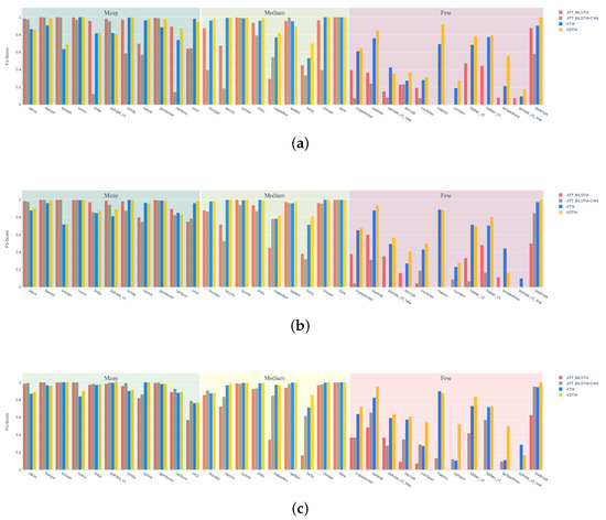
Figure 6. The detailed classification performance of each Domain Generation Algorithm (DGA) category for all comparative models when using a DGA long-tailed distribution dataset with (a) $\alpha =3$, (b) $\alpha =5$, (c) $\alpha =6$.

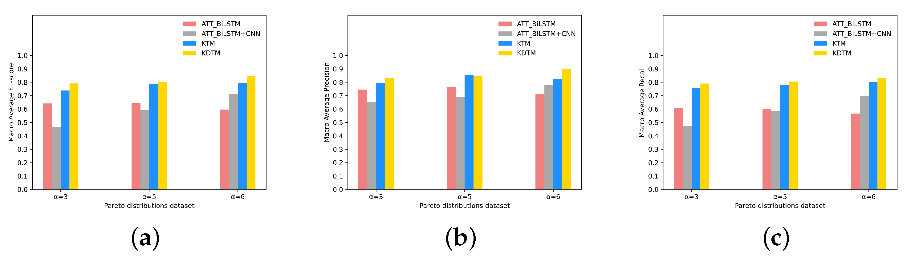
Figure 7 shows all categories of Macro average F1 scores, Macro average precision, and Macro average recall of comparing models on the datasets with different Pareto distributions. From the results, it can be seen that our KDTM model results are optimal on three datasets with different Pareto distributions, demonstrating the robustness of KDTM. As $\alpha$ increases, the overall detection performance of the KDTM model shows an upward trend in the Macro average F1 score. Except for the downward trend of ATT_BiLSTM, other comparative models also show an upward trend. When $\alpha =3$, the optimal result for the Many categories detection appears in ATT_BiLSTM, as $\alpha$ increases, the accuracy of Many, Medium, and Few categories decreases. This indicates that although the amount of data has increased, the increase in imbalance factors has led to a widening gap in the amount of data between the Many and Few categories, resulting in a decrease in accuracy. This is the most common phenomenon in traditional models when encountering imbalanced datasets. ATT_BiLSTM + CNN compared with ATT_BiLSTM, adding CNN can obtain more text features, so as the data volume increases, more information can be obtained. The results showed that the detection results of ATT_BiLSTM + CNN increased with the increase in $\alpha$ in the Many and Medium categories, but there was no significant improvement effect in the Few categories. KTM used transfer learning to transfer the knowledge in the Many categories to the Few categories, so when the amount of data in the Many increases, the knowledge in the relative Few will also increase. KDTM inherits this advantage and retains more of the forgotten knowledge in the Many categories. As the imbalance factor increases and the number of Many categories of data increases, our model will also perform well.

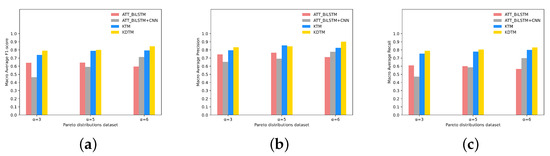
Figure 7. All categories of (a) Macro average F1 scores, (b) Macro average precision, and (c) Macro average recall of comparing models on the datasets with different Pareto distributions.

Table 4 also shows that KDTM has the best overall classification performance and can achieve optimal detection performance for categories belonging to Medium and Few. The accuracy of the corresponding Medium and Few categories will increase as $\alpha$ increases, achieving the optimal result in $\alpha =6$. Specifically, while ensuring that the accuracy of the Many categories is close to the optimal result, the Few categories can also have a significant improvement. Compared with other models in $\alpha =3$, the Few categories’ Macro average F1 score has increased by 28%, 42%, and 9%, respectively, in $\alpha =5$ by 33%, 43%, and 2%, and in $\alpha =6$ by 50%, 32%, and 12%, respectively. In Table 5, we use the Macro average F1 score to compare our model with existing DGA deep learning models. The results show that the overall performance of our model has reached state-of-the-art compared with recent models.

Table 4. Macro average F1 scores on Pareto distribution $\alpha =3$, $\alpha =5$, and $\alpha =6$ datasets. Comparison with the other methods with different metrics. The bolded values are the best in the same metrics, $\alpha$ and data blocks.

Model	Metrics	$\mathit{\alpha }=3$				$\mathit{\alpha }=5$				$\mathit{\alpha }=6$
		Many	Medium	Few	All	Many	Medium	Few	All	Many	Medium	Few	All
ATT_BiLSTM [32]	Precision	0.984	0.873	0.515	0.746	0.972	0.897	0.491	0.766	0.949	0.907	0.344	0.711
	Recall	0.99	0.79	0.36	0.608	0.962	0.772	0.247	0.601	0.918	0.735	0.122	0.565
	F1	0.987	0.797	0.415	0.641	0.967	0.813	0.247	0.645	0.918	0.767	0.167	0.596
ATT_BiLSTM + CNN [26]	Precision	0.983	0.687	0.506	0.652	0.946	0.834	0.367	0.691	0.943	0.889	0.536	0.777
	Recall	0.796	0.683	0.208	0.472	0.916	0.83	0.108	0.585	0.967	0.913	0.287	0.697
	F1	0.808	0.583	0.25	0.464	0.926	0.802	0.142	0.591	0.954	0.898	0.352	0.714
KTM	Precision	0.984	0.836	0.724	0.794	0.955	0.886	0.761	0.855	0.917	0.948	0.652	0.824
	Recall	0.943	0.916	0.58	0.753	0.947	0.938	0.514	0.779	0.946	0.943	0.561	0.799
	F1	0.942	0.87	0.588	0.739	0.948	0.908	0.565	0.787	0.929	0.945	0.558	0.792
KDTM	Precision	0.888	0.901	0.775	0.833	0.963	0.915	0.695	0.844	0.926	0.97	0.836	0.902
	Recall	0.975	0.941	0.633	0.79	0.971	0.933	0.575	0.805	0.954	0.958	0.618	0.829
	F1	0.927	0.916	0.67	0.792	0.966	0.919	0.577	0.801	0.939	0.963	0.674	0.845

Table 5. Comparison of Macro average F1 score between our models and existing Domain Generation Algorithm (DGA) deep learning detection models. The bolded values are the best method and Macro average F1 score.

Method	Year	Macro Average F1 Score
LSTM [14]	2016	0.542
RNN [27]	2017	0.660
SVM and LSTM-based models [28]	2017	0.267
LSTM.MI [36]	2018	0.567
CNN [37]	2019	0.612
B-LSTM/B-RNN/B-GRU [29]	2020	0.470
ATT_BiLSTM [32]	2021	0.837
Extended Character Feature in BiLSTM [31]	2022	0.751
MHSA-RCNN-SABILSTM [33]	2022	0.838
PEPC [39]	2022	0.805
TLM [40]	2023	0.766
KTM	2024	0.792
KDTM	2024	0.845

Overall, the KDTM can significantly improve the detection accuracy of categories with small sample sizes and the overall detection accuracy of the model while ensuring the accuracy of categories with large sample sizes, enabling DGA detection to detect more categories.

5. Conclusions

In this paper, we propose KTM to optimize the long-tailed DGA detection problem. It divides the DGA detection task into multiple stages and uses the DBRM for balancing the data difference at each stage for the long-tailed DGA dataset. KTM uses transfer learning to transfer the knowledge from the big sample categories to the small sample categories stage by stage, which improves the overall accuracy, especially for tail categories. We propose KDTM, which adds knowledge distillation to alleviate catastrophic forgetting from the process of transfer weights. It can also be seen from the experimental results that compared with the traditional deep learning models, our method performs better in the tail categories and our model improves the overall accuracy to 84.5%. We also verify that in the long-tailed DGA detection, multi-stage transfer learning has the best effect by averaging each stage category and dividing the task into two stages. We use three DGA datasets to follow Pareto distributions to verify the generalization of the model by applying the model to datasets with different Pareto distributions. KDTM has a good effect compared with other models in a variety of DGA long-tailed distributions and is more conducive to dealing with changes in data in practical scenarios. KDTM’s more friendly feature towards tail categories can detect newly generated small sample categories, enhancing its defense against hacker attacks. In the future, as many categories in DGA are prone to confusion, we will add feature difference analysis of tail categories to solve the detection confusion caused by feature similarity between categories.

References

- Hoque, N.; Bhattacharyya, D.K.; Kalita, J.K. Botnet in DDoS attacks: Trends and challenges. IEEE Commun. Surv. Tutorials 2015, 17, 2242–2270. [Google Scholar] [CrossRef]
- Feily, M.; Shahrestani, A.; Ramadass, S. A survey of botnet and botnet detection. In Proceedings of the 2009 Third International Conference on Emerging Security Information, Systems and Technologies, Athens, Greece, 18–23 June 2009; pp. 268–273. [Google Scholar]
- Silva, S.S.; Silva, R.M.; Pinto, R.C.; Salles, R.M. Botnets: A survey. Comput. Netw. 2013, 57, 378–403. [Google Scholar] [CrossRef]
- Curts, R.J.; Campbell, D.E. Rethinking Command & Control. In Proceedings of the 2006 Command and Control Research and Technology Symposium, San Diego, CA, USA, 20–22 June 2006. [Google Scholar]
- Zargar, S.T.; Joshi, J.; Tipper, D. A survey of defense mechanisms against distributed denial of service (DDoS) flooding attacks. IEEE Commun. Surv. Tutorials 2013, 15, 2046–2069. [Google Scholar] [CrossRef]
- Cormack, G.V. Email spam filtering: A systematic review. Found. Trends® Inf. Retr. 2008, 1, 335–455. [Google Scholar] [CrossRef]
- Odlyzko, A.M. Internet traffic growth: Sources and implications. In Optical Transmission Systems and Equipment for WDM Networking II; SPIE: Bellingham, WA, USA, 2003; Volume 5247, pp. 1–15. [Google Scholar]
- Antonakakis, M.; Perdisci, R.; Nadji, Y.; Vasiloglou, N.; Dagon, D. From Throw-Away Traffic to Bots: Detecting the Rise of DGA-Based Malware. In Proceedings of the Usenix Conference on Security Symposium, Bellevue, WA, USA, 8–10 August 2012. [Google Scholar]
- Stone-Gross, B.; Cova, M.; Cavallaro, L.; Gilbert, B.; Szydlowski, M. Your Botnet is My Botnet: Analysis of a Botnet Takeover. In Proceedings of the 2009 ACM Conference on Computer and Communications Security, CCS 2009, Chicago, IL, USA, 9–13 November 2009. [Google Scholar]
- Davuth, N.; Kim, S.R. Classification of Malicious Domain Names using Support Vector Machine and Bi-gram Method. Int. J. Secur. Its Appl. 2013, 7, 51–58. [Google Scholar]
- Bilge, L.; Kirda, E.; Kruegel, C.; Balduzzi, M. EXPOSURE: Finding Malicious Domains Using Passive DNS Analysis. In Proceedings of the Network and Distributed System Security Symposium, NDSS 2011, San Diego, CA, USA, 6–9 February 2011. [Google Scholar]
- Zhou, Y.L.; Li, Q.S.; Miao, Q.; Team, C.; Beijing; Yim, K. DGA-Based Botnet Detection Using DNS Traffic. J. Internet Serv. Inf. Secur. 2013, 3, 116–123. [Google Scholar]
- Anderson, H.S.; Woodbridge, J.; Filar, B. DeepDGA: Adversarially-Tuned Domain Generation and Detection. In Proceedings of the 2016 ACM Workshop on Artificial Intelligence and Security 2016, Vienna, Austria, 28 October 2016. [Google Scholar]
- Woodbridge, J.; Anderson, H.S.; Ahuja, A.; Grant, D. Predicting Domain Generation Algorithms with Long Short-Term Memory Networks. arXiv 2016, arXiv:1611.00791. [Google Scholar]
- Yu, B.; Gray, D.L.; Jie, P.; Cock, M.; Nascimento, A. Inline DGA Detection with Deep Networks. In Proceedings of the IEEE International Conference on Data Mining Workshops, New Orleans, LA, USA, 18–21 November 2017. [Google Scholar]
- Chen, Y.; Zhang, S.; Liu, J.; Li, B. Towards a Deep Learning Approach for Detecting Malicious Domains. In Proceedings of the 2018 IEEE International Conference on Smart Cloud (SmartCloud), New York, NY, USA, 21–23 September 2018; pp. 190–195. [Google Scholar]
- Zhang, Z.; Pfister, T. Learning fast sample re-weighting without reward data. In Proceedings of the IEEE/CVF International Conference on Computer Vision, Montreal, BC, Canada, 11–17 October 2021; pp. 725–734. [Google Scholar]
- Yin, X.; Yu, X.; Sohn, K.; Liu, X.; Chandraker, M. Feature transfer learning for face recognition with under-represented data. In Proceedings of the IEEE/CVF Conference on Computer Vision and Pattern Recognition, Long Beach, CA, USA, 16–17 June 2019; pp. 5704–5713. [Google Scholar]
- Hinton, G.; Vinyals, O.; Dean, J. Distilling the knowledge in a neural network. arXiv 2015, arXiv:1503.02531. [Google Scholar]
- Tuan, T.A.; Anh, N.V.; Luong, T.T.; Long, H.V. UTL_DGA22-a dataset for DGA botnet detection and classification. Comput. Netw. 2023, 221, 109508. [Google Scholar] [CrossRef]
- Yadav, S.; Reddy, A.K.K.; Reddy, A.N.; Ranjan, S. Detecting algorithmically generated malicious domain names. In Proceedings of the 10th ACM SIGCOMM Conference on Internet Measurement, Melbourne, Australia, 1–3 November 2010; pp. 48–61. [Google Scholar]
- Wang, W.; Shirley, K. Breaking bad: Detecting malicious domains using word segmentation. arXiv 2015, arXiv:1506.04111. [Google Scholar]
- Hsu, C.H.; Huang, C.Y.; Chen, K.T. Fast-flux bot detection in real time. In Proceedings of the Recent Advances in Intrusion Detection: 13th International Symposium, RAID 2010, Ottawa, ON, Canada, 15–17 September 2010; Proceedings 13. Springer: Berlin/Heidelberg, Germany, 2010; pp. 464–483. [Google Scholar]
- Zaremba, W.; Sutskever, I.; Vinyals, O. Recurrent neural network regularization. arXiv 2014, arXiv:1409.2329. [Google Scholar]
- Tuan, T.A.; Long, H.V.; Taniar, D. On detecting and classifying DGA botnets and their families. Comput. Secur. 2022, 113, 102549. [Google Scholar] [CrossRef]
- Ren, F.; Jiang, Z.; Wang, X.; Liu, J. A DGA domain names detection modeling method based on integrating an attention mechanism and deep neural network. Cybersecurity 2020, 3, 4. [Google Scholar] [CrossRef]
- Lison, P.; Mavroeidis, V. Automatic detection of malware-generated domains with recurrent neural models. arXiv 2017, arXiv:1709.07102. [Google Scholar]
- Mac, H.; Tran, D.; Tong, V.; Nguyen, L.G.; Tran, H.A. DGA botnet detection using supervised learning methods. In Proceedings of the 8th International Symposium on Information and Communication Technology, Nha Trang, Vietnam, 7–8 December 2017; pp. 211–218. [Google Scholar]
- Ravi, V.; Alazab, M.; Srinivasan, S.; Arunachalam, A.; Soman, K. Adversarial defense: DGA-based botnets and DNS homographs detection through integrated deep learning. IEEE Trans. Eng. Manag. 2021, 70, 249–266. [Google Scholar] [CrossRef]
- Ren, F.; Jiang, Z.; Liu, J. Integrating an attention mechanism and deep neural network for detection of DGA domain names. In Proceedings of the 2019 IEEE 31st International Conference on Tools with Artificial Intelligence (ICTAI), Portland, OR, USA, 4–6 November 2019; pp. 848–855. [Google Scholar]
- Pan, R.; Chen, J.; Ma, H.; Bai, X. Using extended character feature in Bi-LSTM for DGA domain name detection. In Proceedings of the 2022 IEEE/ACIS 22nd International Conference on Computer and Information Science (ICIS), Zhuhai, China, 26–28 June 2022; pp. 115–118. [Google Scholar]
- Namgung, J.; Son, S.; Moon, Y.S. Efficient Deep Learning Models for DGA Domain Detection. Secur. Commun. Netw. 2021, 2021. [Google Scholar] [CrossRef]
- Sarojini, S.; Asha, S. Detection for domain generation algorithm (DGA) domain botnet based on neural network with multi-head self-attention mechanisms. Int. J. Syst. Assur. Eng. Manag. 2022, 1–16. [Google Scholar] [CrossRef]
- Cui, Y.; Jia, M.; Lin, T.Y.; Song, Y.; Belongie, S. Class-balanced loss based on effective number of samples. In Proceedings of the IEEE/CVF Conference on Computer Vision and Pattern Recognition, Long Beach, CA, USA, 15–20 June 2019; pp. 9268–9277. [Google Scholar]
- Calvo, R.A.; Lee, J.M. Coping with the news: The machine learning way. In Proceedings of the AusWEB 2003, Gold Coast, Australian, 5–9 July 2003. [Google Scholar]
- Tran, D.; Mac, H.; Tong, V.; Tran, H.A.; Nguyen, L.G. A LSTM based framework for handling multiclass imbalance in DGA botnet detection. Neurocomputing 2018, 275, 2401–2413. [Google Scholar] [CrossRef]
- Zhou, S.; Lin, L.; Yuan, J.; Wang, F.; Ling, Z.; Cui, J. CNN-based DGA detection with high coverage. In Proceedings of the 2019 IEEE International Conference on Intelligence and Security Informatics (ISI), Shenzhen, China, 1–3 July 2019; pp. 62–67. [Google Scholar]
- Simran, K.; Balakrishna, P.; Vinayakumar, R.; Soman, K. Deep learning based frameworks for handling imbalance in DGA, Email, and URL Data Analysis. In Proceedings of the Computational Intelligence, Cyber Security and Computational Models. Models and Techniques for Intelligent Systems and Automation: 4th International Conference, ICC3 2019, Coimbatore, India, 19–21 December 2019; Springer: Singapore, 2020; pp. 93–104. [Google Scholar]
- Huang, W.; Zong, Y.; Shi, Z.; Wang, L.; Liu, P. PEPC: A Deep Parallel Convolutional Neural Network Model with Pre-trained Embeddings for DGA Detection. In Proceedings of the 2022 International Joint Conference on Neural Networks (IJCNN), Padua, Italy, 18–23 July 2022; pp. 1–8. [Google Scholar]
- Fan, B.; Liu, Y.; Cuthbert, L. Improvement of DGA Long Tail Problem Based on Transfer Learning. In Computer and Information Science; Lee, R., Ed.; Springer International Publishing: Cham, Switzerland, 2023; pp. 139–152. [Google Scholar] [CrossRef]
- Pouyanfar, S.; Tao, Y.; Mohan, A.; Tian, H.; Kaseb, A.S.; Gauen, K.; Dailey, R.; Aghajanzadeh, S.; Lu, Y.H.; Chen, S.C.; et al. Dynamic sampling in convolutional neural networks for imbalanced data classification. In Proceedings of the 2018 IEEE conference on multimedia information processing and retrieval (MIPR), Miami, FL, USA, 10–12 April 2018; pp. 112–117. [Google Scholar]
- He, H.; Garcia, E.A. Learning from imbalanced data. IEEE Trans. Knowl. Data Eng. 2009, 21, 1263–1284. [Google Scholar]
- Ren, J.; Yu, C.; Sheng, S.; Ma, X.; Zhao, H.; Yi, S.; Li, H. Balanced meta-softmax for long-tailed visual recognition. arXiv 2020, arXiv:2007.10740. [Google Scholar]
- Wang, Y.X.; Ramanan, D.; Hebert, M. Learning to model the tail. In Proceedings of the 31st International Conference on Neural Information Processing Systems, Long Beach, CA, USA, 4–9 December 2017; pp. 7032–7042. [Google Scholar]
- Chu, P.; Bian, X.; Liu, S.; Ling, H. Feature space augmentation for long-tailed data. In Proceedings of the Computer Vision–ECCV 2020: 16th European Conference, Glasgow, UK, 23–28 August 2020; Proceedings, Part XXIX 16. Springer: Cham, Switzerland, 2020; pp. 694–710. [Google Scholar]
- Wang, J.; Lukasiewicz, T.; Hu, X.; Cai, J.; Xu, Z. RSG: A Simple but Effective Module for Learning Imbalanced Datasets. In Proceedings of the IEEE/CVF Conference on Computer Vision and Pattern Recognition, Nashville, TN, USA, 20–25 June 2021; pp. 3784–3793. [Google Scholar]
- Pan, S.J.; Yang, Q. A survey on transfer learning. IEEE Trans. Knowl. Data Eng. 2009, 22, 1345–1359. [Google Scholar] [CrossRef]
- Tan, C.; Sun, F.; Kong, T.; Zhang, W.; Yang, C.; Liu, C. A survey on deep transfer learning. In Proceedings of the International Conference on Artificial Neural Networks, Rhodes, Greece, 4–7 October 2018; Springer: Cham, Switzerland, 2018; pp. 270–279. [Google Scholar]
- Ma, H.; Ng, B.K.; Lam, C.T. PK-BERT: Knowledge Enhanced Pre-trained Models with Prompt for Few-Shot Learning. In Computer and Information Science; Lee, R., Ed.; Springer International Publishing: Cham, Switzerland, 2023; pp. 31–44. [Google Scholar] [CrossRef]
- Liu, J.; Sun, Y.; Han, C.; Dou, Z.; Li, W. Deep representation learning on long-tailed data: A learnable embedding augmentation perspective. In Proceedings of the IEEE/CVF Conference on Computer Vision and Pattern Recognition, Seattle, WA, USA, 13–19 June 2020; pp. 2970–2979. [Google Scholar]
- Liu, B.; Li, H.; Kang, H.; Hua, G.; Vasconcelos, N. Gistnet: A geometric structure transfer network for long-tailed recognition. In Proceedings of the IEEE/CVF International Conference on Computer Vision, Montreal, BC, Canada, 11–17 October 2021; pp. 8209–8218. [Google Scholar]
- Lee, S.W.; Kim, J.H.; Jun, J.; Ha, J.W.; Zhang, B.T. Overcoming catastrophic forgetting by incremental moment matching. Adv. Neural Inf. Process. Syst. 2017, 30, e08475. [Google Scholar] [CrossRef]
- Gou, J.; Yu, B.; Maybank, S.J.; Tao, D. Knowledge distillation: A survey. Int. J. Comput. Vis. 2021, 129, 1789–1819. [Google Scholar] [CrossRef]
- Hu, X.; Jiang, Y.; Tang, K.; Chen, J.; Miao, C.; Zhang, H. Learning to segment the tail. In Proceedings of the IEEE/CVF Conference on Computer Vision and Pattern Recognition, Seattle, WA, USA, 13–19 June 2020; pp. 14045–14054. [Google Scholar]
- Xiang, L.; Ding, G.; Han, J. Learning from multiple experts: Self-paced knowledge distillation for long-tailed classification. In Proceedings of the European Conference on Computer Vision, Glasgow, UK, 23–28 August 2020; Springer: Cham, Switzerland, 2020; pp. 247–263. [Google Scholar]
- Wang, X.; Lian, L.; Miao, Z.; Liu, Z.; Yu, S.X. Long-tailed recognition by routing diverse distribution-aware experts. arXiv 2020, arXiv:2010.01809. [Google Scholar]
- Arnold, B.C. Pareto distribution. Wiley StatsRef Stat. Ref. Online 2014, 1–10. [Google Scholar] [CrossRef]
- Weston, J.; Ratle, F.; Mobahi, H.; Collobert, R. Deep Learning via Semi-supervised Embedding. In Proceedings of the 25th International Conference on Machine Learning, Edinburgh, UK, 26 June 26–1 July 2012. [Google Scholar]
- Zhang, J.; Tao, D. Empowering things with intelligence: A survey of the progress, challenges, and opportunities in artificial intelligence of things. IEEE Internet Things J. 2020, 8, 7789–7817. [Google Scholar] [CrossRef]
- Niu, Z.; Zhong, G.; Yu, H. A review on the attention mechanism of deep learning. Neurocomputing 2021, 452, 48–62. [Google Scholar] [CrossRef]
- Jang, E.; Gu, S.; Poole, B. Categorical reparameterization with gumbel-softmax. arXiv 2016, arXiv:1611.01144. [Google Scholar]
- Censor, B.Y. Proximity Function Minimization Using Multiple Bregman Projections, with Applications to Split Feasibility and Kullback–Leibler Distance Minimization. Ann. Oper. Res. 2001, 105, 77–98. [Google Scholar]
- Ye, J. Single valued neutrosophic cross-entropy for multicriteria decision making problems. Appl. Math. Model. 2014, 38, 1170–1175. [Google Scholar] [CrossRef]
- Salakhutdinov, R.; Hinton, G.E. Replicated Softmax: An Undirected Topic Model. In Proceedings of the International Conference on Neural Information Processing Systems, Vancouver, BC, Canada, 7–10 December 2009. [Google Scholar]
- Pang, B.; Nijkamp, E.; Wu, Y.N. Deep learning with tensorflow: A review. J. Educ. Behav. Stat. 2020, 45, 227–248. [Google Scholar] [CrossRef]
- Kingma, D.P.; Ba, J. Adam: A method for stochastic optimization. arXiv 2014, arXiv:1412.6980. [Google Scholar]
- Tang, J.; Shivanna, R.; Zhao, Z.; Lin, D.; Singh, A.; Chi, E.H.; Jain, S. Understanding and improving knowledge distillation. arXiv 2020, arXiv:2002.03532. [Google Scholar]
Disclaimer/Publisher’s Note: The statements, opinions and data contained in all publications are solely those of the individual author(s) and contributor(s) and not of MDPI and/or the editor(s). MDPI and/or the editor(s) disclaim responsibility for any injury to people or property resulting from any ideas, methods, instructions or products referred to in the content. |
© 2024 by the authors. Licensee MDPI, Basel, Switzerland. This article is an open access article distributed under the terms and conditions of the Creative Commons Attribution (CC BY) license (https://creativecommons.org/licenses/by/4.0/).