1. Introduction
Consider the linear matrix equation
where
and
. The solution
X of (
1) is called the inner inverse of
A. For arbitrary
, all the inner inverses of
A can be expressed as
where
is the Moore–Penrose generalized inverse of
A.
Inner inverses play a role in solving systems of linear equations, finding solutions to least squares problems, and characterizing the properties of linear transformations [
1]. They are also useful in various areas of engineering, such as robotics, big data analysis, network learning, sensory fusion, and so on [
2,
3,
4,
5,
6].
To calculate the inner inverse of a matrix, various methods can be used, such as the Moore–Penrose pseudoinverse, singular value decomposition (SVD), or the method of partitioned matrices [
1]. To our knowledge, few people discuss numerical methods for solving all the inner inverses of a matrix. In [
7], the authors designed an iterative method based on gradient (GBMC) to solve the matrix Equation (
1), which has the following iterative formula:
Here,
is called the convergence factor. If the initial matrix
, then the sequence
converges to
. Recently, various nonlinear and linear recurrent neural network (RNN) models have been developed for computing the pseudoinverse of any rectangular matrices (for more details, see [
8,
9,
10,
11]). The gradient-based neural network (GNN), whose derivation is based on the gradient of an nonnegative energy function, is an alternative for calculating the Moore–Penrose generalized inverses [
12,
13,
14,
15]. These methods for solving the inner inverses and for other generalized inverses of a matrix frequently use the matrix–matrix product operation, and consume a lot of computing time. In this paper, we aimed to explore two block Kaczmarz methods to solve (
1) by the product of the matrix and vector.
In this paper, we denote
,
,
,
,
and
as the conjugate transpose, the Moore–Penrose pseudoinverse, the inner inverse, the 2-norm, the Frobenius norm of
A and the inner product of two matrices
A and
B, respectively. In addition, for a given matrix
,
,
,
,
and
, are used to denote its
ith row,
jth column, the column space of
A, the maximum singular value and the smallest nonzero singular value of
A, respectively. Recall that
and
. For an integer
, let
. Let
denote the expected value conditional on the first k iterations; that is,
where
is the column chosen at the
sth iteration.
The rest of this paper is organized as follows. In
Section 2, we derive the projected randomized block Kaczmarz method (MII-PRBK) for finding the inner inverses of a matrix and give its theoretical analysis. In
Section 3, we discuss the randomized average block Kaczmarz method (MII-RABK) and its convergence results. In
Section 4, some numerical examples are provided to illustrate the effectiveness of the proposed methods. Finally, some brief concluding remarks are described in
Section 5.
2. Projected Randomized Block Kaczmarz Method for Inner Inverses of a Matrix
The classical Kaczmarz method is a row iterative scheme for solving the linear consistent system
that requires only
cost per iteration and storage and has a linear rate of convergence [
16]. At each step, the method projects the current iteration onto the solution space of a single constraint. In this section, we are concerned with the randomized Kaczmarz method to solve the matrix Equation (
1). At the
kth iteration, we find the next iterate
that is closest to the current iteration
in the Frobenius norm under the
ith condition
. Hence,
is the optimal solution of the following constrained optimization problem:
Using the Lagrange multiplier method, turn (
2) into the unconstrained optimization problem
Differentiating Lagrangian function
with respect to
X and setting to zero gives
. Substituting into (
3) and differentiating
with respect to
Y, we can obtain
. So, the projected randomized block Kaczmarz for solving
iterates as
where
is selected with probability
. We describe this method as Algorithm 1, which is called the MII-PRBK algorithm.
| Algorithm 1 Projected randomized block Kaczmarz method for matrix inner inverses (MII-PRBK) |
Input: , - 1:
for do - 2:
Pick i with probability - 3:
Compute - 4:
end for
|
The following lemmas will be used extensively in this paper. Their proofs are straightforward.
Lemma 1. Let be given. For any vector , it holds that Lemma 2 ([
17]).
Let be given. For any matrix , if , it holds that Using Lemma 2 twice, and the fact , we can obtain Lemma 3.
Lemma 3. Let be given. For any matrix , if and , it holds that Remark 1. Lemma 3 can be seen as a special case of Lemma 1 in [18]. That is, let For any matrix , it holds Notice that is well defined because and . Theorem 1. The sequence generated by the MII-PRBK method starting from any initial matrix converges linearly to in the mean square form. Moreover, the solution error in expectation for the iteration sequence obeyswhere . Proof. For
, by (
4) and
, we can obtain
and
Combining (
9), (
10) and
, it follows from
and
that
By taking the conditional expectation, we have
The second inequality is obtained by Lemma 3 because and on induction.
By the law of total expectation, we have
This completes the proof. □
3. Randomized Average Block Kaczmarz Method for Inner Inverses of a Matrix
In practice, the main drawback of (
4) is that each iteration is expensive and difficult to parallelize, since the Moore–Penrose inverse
is needed to compute. In addition,
is unknown or too large to store in some practical problem. It is necessary to develop the pseudoinverse-free methods to compute the inner inverses of large-scale matrices. In this section, we exploit the average block Kaczmarz method [
16,
19] for solving linear equations to matrix equations.
At each iteration, the PRBK method (
4) does an orthogonal projection of the current estimate matrix
onto the corresponding hyperplane
. Next, instead of projecting on the hyperplane
, we consider the approximate solution
by projecting the current estimate
onto the hyperplane
. That is,
Then, we take a convex combination of all directions
(the weight is
) with some stepsize
, and obtain the following average block Kaczmarz method:
Setting
, we obtain the following randomized block Kaczmarz iteration
where
is selected with probability
. The cost of each iteration of this method is
if the square of the row norm of
A has been calculated in advance. We describe this method as Algorithm 2, which is called the MII-RABK algorithm.
| Algorithm 2 Randomized average block Kaczmarz method for matrix inner inverses (MII-RABK) |
Input: , and - 1:
for do - 2:
Pick i with probability - 3:
Compute - 4:
end for
|
In the following theorem, with the idea of the RK method [
20], we show that the iteration (
11) converges linearly to the matrix
for any initial matrix
.
Theorem 2. Assume . The sequence generated by the MII-RABK method starting from any initial matrix converges linearly to in mean square form. Moreover, the solution error in expectation for the iteration sequence obeyswhere . Proof. For
, by (
11) and
, we have
then
By taking the conditional expectation, we have
Noting that
and
, we have
by induction. Then, by Lemma 3 and
, we can obtain
Finally, by (
13) and induction on the iteration index
k, we obtain the estimate (
12). This completes the proof. □
Remark 2. If or , then , which is the unique minimum norm least squares solution of (2). Theorems 1 and 2 imply that the sequence generated by the MII-PRBK or MII-RABK method with or converges linearly to . Remark 3. Noting thatthis means that the convergence factor of the MII-PRBK method is smaller than that of MII-RABK method. However, in practice, it is very expensive to calculate the pseudoinverse of large-scale matrices. Remark 4. Replacing in (11) with , we obtain the following relaxed projected randomized block Kaczmarz method (MII-PRBKr)where is the step size, and i is selected with probability . By the similar approach as used in the proof of Theorem 2, we can prove that the iteration satisfies the following estimatewhere . It is obvious that when , the MII-PRBKr iteration (14) is actually the MII-PRBK iteration (4). 4. Numerical Experiments
In this section, we will present some experiment results of the proposed algorithms for solving the inner inverse, and compare them with GBMC [
7] for rectangular matrices. All experiments are carried out by using MATLAB (version R2020a) in a personal computer with Intel(R) Core(TM) i7-4712MQ CPU @2.30 GHz, RAM 8 GB and Windows 10.
All computations are started with the random matrices
, and terminated once the relative error (RE) of the solution, defined by
at the current iteration
, satisfies
or exceeds the maximum iteration
. We report the average number of iterations (denoted as “IT”) and the average computing time in seconds (denoted as“CPU”) for 10 trials repeated runs of the MII-PRBK and MII-RABK methods. For clarity, we restate three methods as follows.
We underscore once again the difference between the two algorithms; that is, Algorithm 1 needs the Moore–Penrose generalized inverse , whereas Algorithm 2 replaces with (which is easier to implement) and adds a stepsize parameter .
Example 1. For given , the entries of A are generated from a standard normal distribution by a Matlab built-in function, i.e., or .
Firstly, we test the impact of
in the MII-RABK method on the experimental results. To do this, we vary
from
to
by step
, where
satisfies
in Theorem 2.
Figure 1 plots the IT and CPU versus different
with different matrices in
Table 1. From
Figure 1, it can be seen that the number of iteration steps and the running time first decrease and then increase with the increase in
, and almost achieve the minimum value when
for all matrices. Therefore, we set
in this example.
The results of numerical experiments are listed in
Table 1 and
Table 2. From these tables, it can be seen that the MII-GMBC method has the least number of iteration steps, whereas the MII-PRBK method has the least running time.
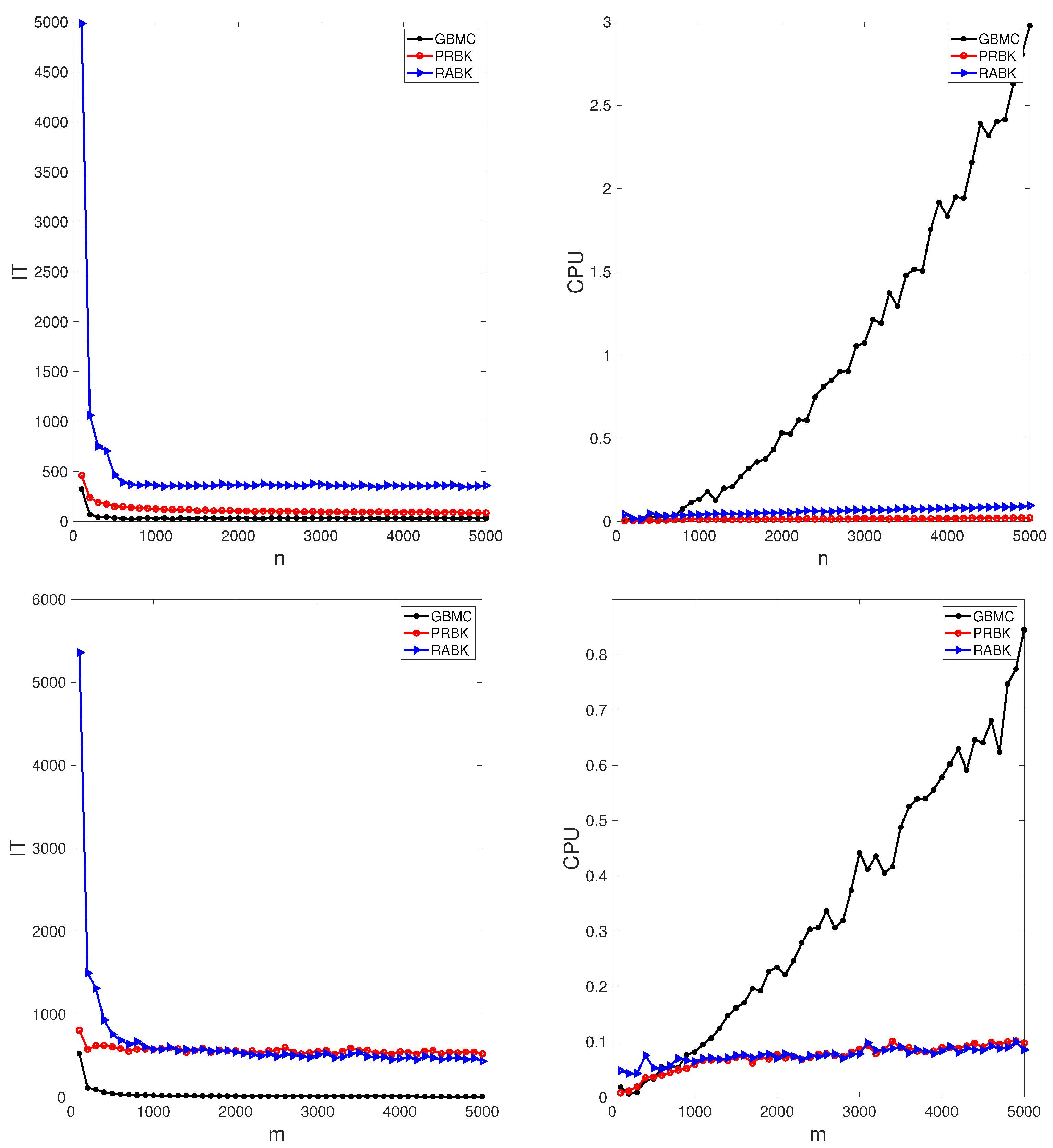
Figure 2 plots the iteration steps and running time of different methods with the matrices
(top) and
(bottom). It is pointed out that the initial points on the left plots (i.e.,
and
) indicate that the MII-RABK method requires a very large number of iteration steps, which is related to Kaczmarz’s anomaly [
21]. That is, the MII-RABK method enjoys a faster rate of convergence in the case where
m is considerably smaller or larger than
n. However, the closer
m and
n are, the slower the convergence is. As the number of rows or columns increases, the iteration steps and runtime of the MII-PRBK and MII-RABK methods are increasing relatively slowly, while the runtime of the GMBC method grows dramatically (see the right plots in
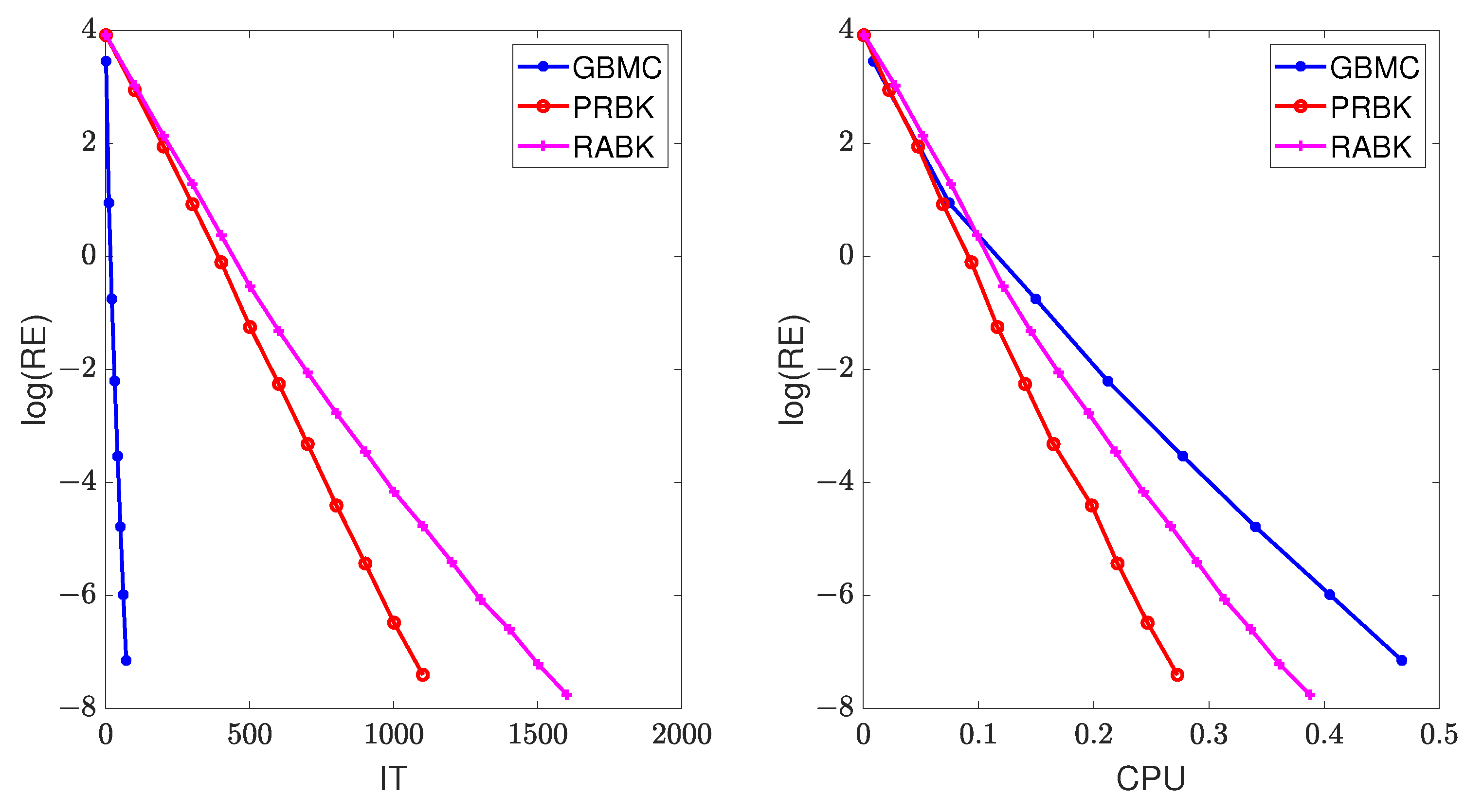
Figure 2). Therefore, our proposed methods are more suitable for large matrices. The curves of relative error
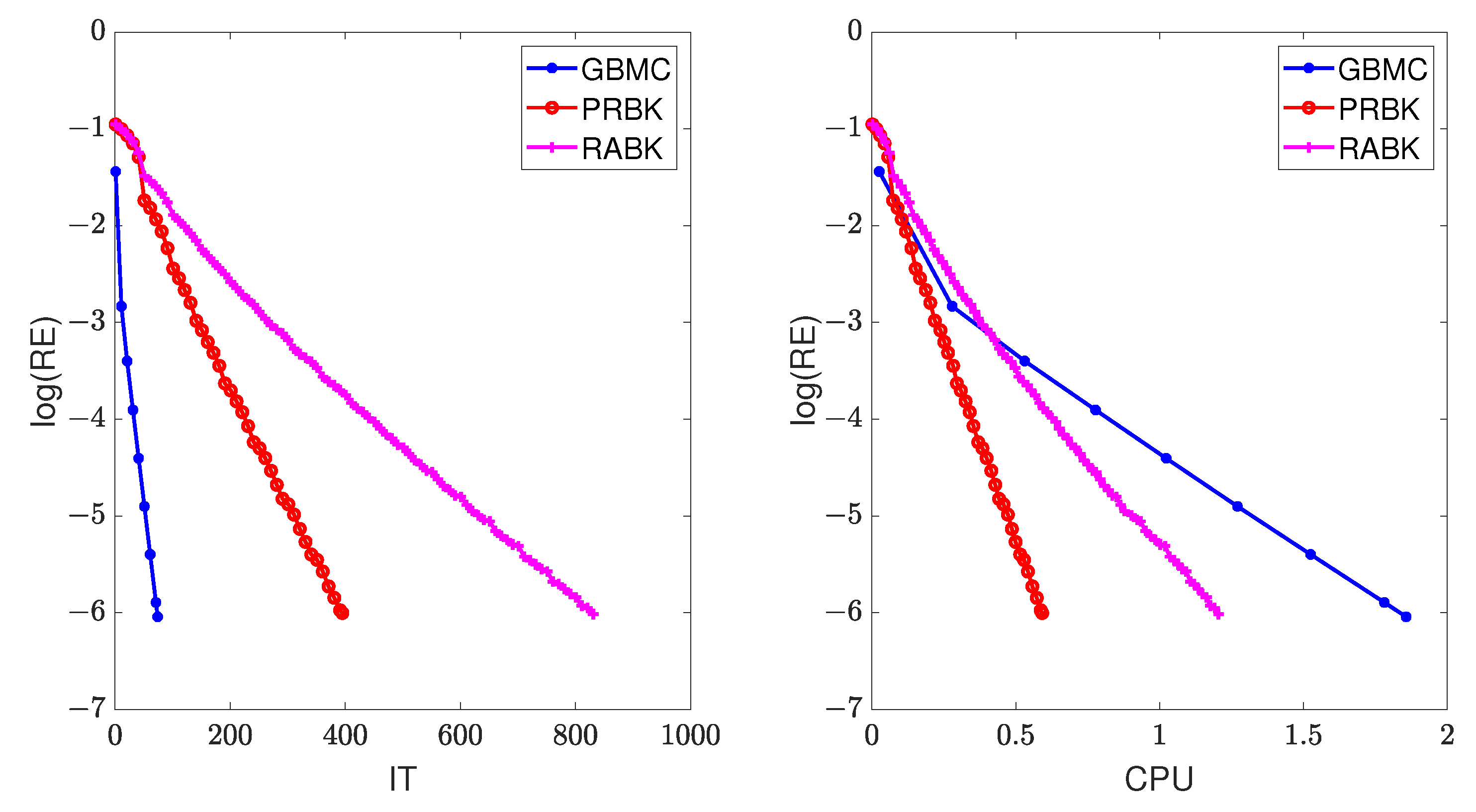
versus the number of iterations “IT” and running time “CPU”, given by the GMBC, MII-PRBK, MII-RABK methods for
, are shown in
Figure 3. From
Figure 3, it can be seen that the relative error of GBMC method decays the fastest when the number of iterations increases and the relative error of MII-PRBK decays the fastest when the running time grows. This is because at each iteration, the GMBC method requires matrix multiplication which involves
flopping operations, whereas the MII-PRBK and MII-RABK methods only cost
flops.
Example 2. For given , the sparse matrix A is generated by a Matlab built-in function , with approximately normally distributed nonzero entries. The input parameters d and are the percentage of nonzeros and the reciprocal of condition number, respectively. In this example, or .
In this example, we set
. The numerical results of IT and CPU are listed in
Table 3 and
Table 4, and the curves of relative error versus IT and CPU are drawn in
Figure 4. From
Table 3 and
Table 4, we can observe that the MII-PRBK method has the least iteration steps and running time. The computational efficiency of the MII-PRBK and MII-RABK methods has been improved by at least 33 and 7 times compared to the GBMC method. Moreover, the advantages of the proposed methods are more pronounced when the matrix size increases.
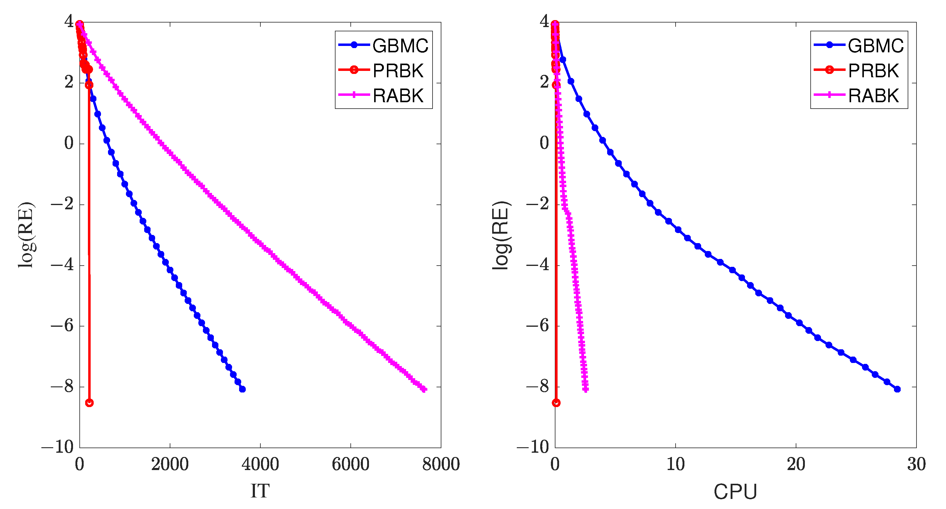
Example 3. Consider dense Toeplitz matrices. For given , or .
In this example, we set . The numerical results of IT and CPU are listed in Table 5, and the curves of the relative error versus IT and CPU are drawn in Figure 5. We can observe the same phenomenon as that in Example 1. Example 4. Consider sparse Toeplitz matrices. For given , or .
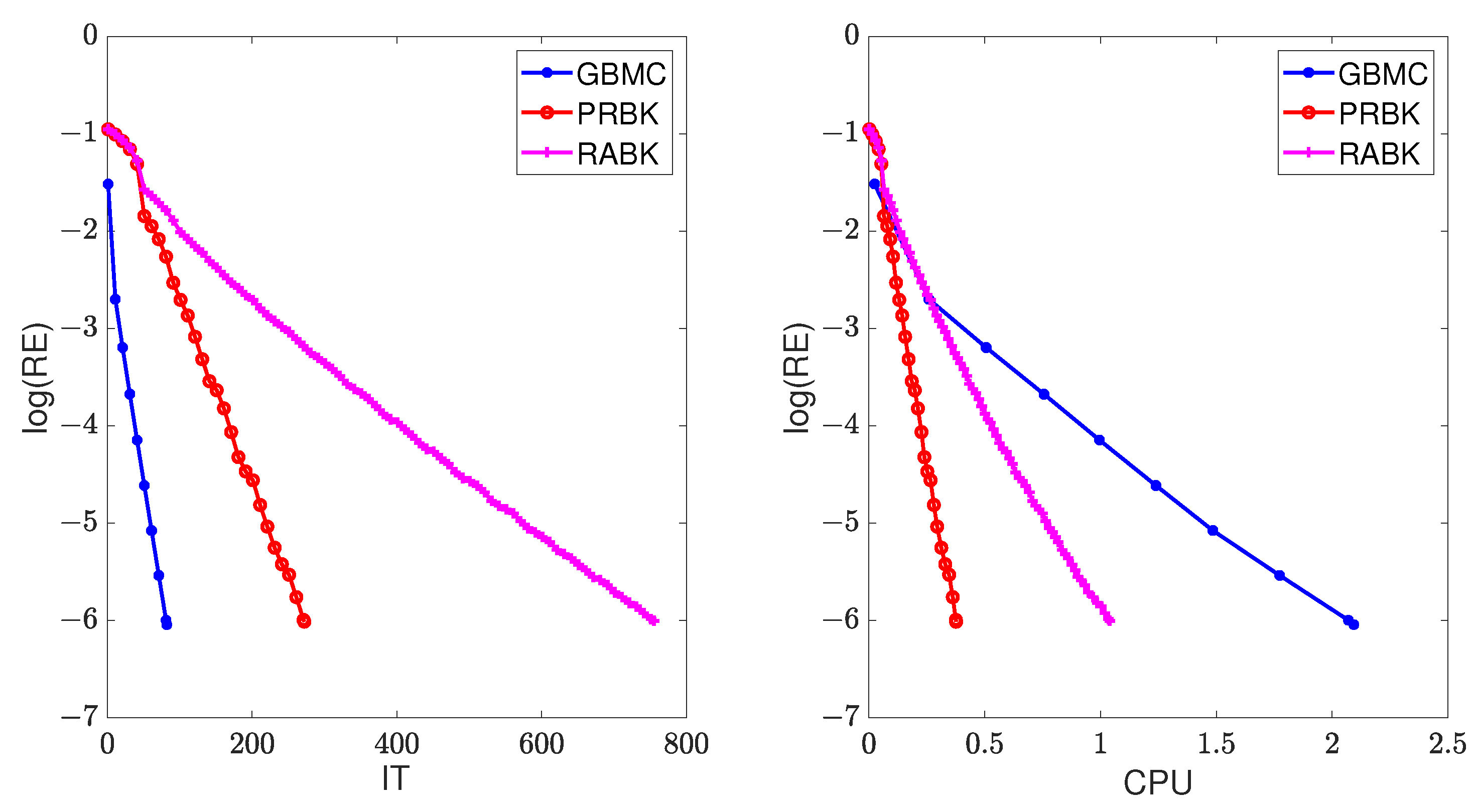
In this example, we set
. The numerical results of IT and CPU are listed in
Table 6, and the curves of the relative error versus IT and CPU are drawn in
Figure 6. Again, we can draw the same conclusion as that in Example 1.


