A New Random Coefficient Autoregressive Model Driven by an Unobservable State Variable

Abstract

A novel random coefficient autoregressive model is proposed, and a feature of the model is the non-stationarity of the state equation. The autoregressive coefficient is an unknown function with an unobservable state variable, which can be estimated by the local linear regression method. The iterative algorithm is constructed to estimate the parameters based on the ordinary least squares method. The ordinary least squares residuals are used to estimate the variances of the errors. The Kalman-smoothed estimation method is used to estimate the unobservable state variable because of its ability to deal with non-stationary stochastic processes. These methods allow deriving the analytical solutions. The performance of the estimation methods is evaluated through numerical simulation. The model is validated using actual time series data from the S&P/HKEX Large Cap Index.

1. Introduction

Autoregressive (AR) models constitute a pivotal class within the realm of time series analysis and have found extensive applications across various domains, including economics, finance, industry, and meteorology. The traditional AR model, with fixed autoregressive coefficients, has seen rapid advancements. However, in the process of solving practical problems, observational data are often characterized as nonlinear and dynamic, which cannot be explained by traditional AR models. By introducing random coefficients, the parameters of the model are allowed to change over time. This makes the models better adapt to the characteristics and changes in complex data, thereby enhancing the model’s fitting and predictive capabilities. This research has attracted wide interest among statisticians and scholars in related fields. The references to nonlinear time series are burgeoning. Notably, a well-known class of nonlinear AR models is random coefficient AR (RCAR) models. A study by Nicholls and Quinn (1982) [1] contained a detailed study of RCAR models, including statistical properties of the model, estimation methods, and hypothesis testing. Based on this foundation, Aue et al. (2006) [2] proposed the quasi-maximum likelihood method for estimating the parameters of an RCAR(1) process. Zhao et al. (2015) [3] investigated the parameter estimation of the RCAR model and its limiting properties under a sequence of martingale errors. This work was subsequently expanded by Horváth and Trapani (2016) [4] to encompass panel data, broadening the applicability of the theory. Most recently, Proia and Soltane (2018) [5] introduced an RCAR process in which the coefficients are correlated. Regis (2022) [6] presented a structured overview of the literature on RCAR models. The autoregressive coefficient discussed in Regis (2022) [6] incorporates a stochastic process, which is a characteristic also shared by our model. However, a key distinction lies in the time-varying nature of the random coefficient’s variance in our model. Furthermore, the existing structure in Regis (2022) [6] to which our model relates is the Dynamic Factor Model (DFM) mentioned in Section 6.2 of Regis (2022) [6]. The DFM consists of three equations relating to an observation, an unobservable latent process, and a time-varying parameter. Similarly, both models incorporate a state variable evolving as a random walk. The difference is that in the DFM the latent process has a linear time-varying autoregressive (TV-AR) structure, whereas in our model it is the observed process that has a nonlinear TV-AR structure. In this regard, the proposed model is at a higher level than the existing structures. This research introduces a novel model aimed at addressing gaps in the existing literature, with an enhanced ability to handle non-stationarity and non-linearity. By leveraging the strengths of multiple approaches, the proposed model offers a more robust framework for capturing the inherent complexity of the data. Moreover, the conventional nonparametric autoregressive models were discussed by Härdle et al. (1998) [7], Kreiss and Neumann (1998) [8], and Vogt (2012) [9], where the nonparametric component is typically related to past observational variables. It is important to note that, despite their nonlinear nature, these models are fundamentally based on stationary processes.

Differing from the aforementioned, this paper presents a nonlinear, non-stationary AR model. There has been some work on non-stationary RCAR models. For instance, Berkes et al. (2009) [10] considered a non-stationary RCAR(1) model by controlling the log expectation of the random coefficients. They demonstrated that, under such conditions, the variance of the error term cannot be estimated via the quasi-maximum-likelihood method, while proving the asymptotic normality of the quasi-maximum-likelihood estimators for the other parameters. Subsequently, Aue and Horváth (2011) [11] proposed a unified quasi-likelihood estimation procedure for both the stationary and non-stationary cases of the model. By contrast, our model features an autoregressive coefficient represented as a potentially nonlinear unknown function. Additionally, its argument at each time-point is defined by a non-stationary unobservable state equation. While the estimation process becomes more intricate, it significantly broadens the model’s applicability. Our model is also regarded as a novel random coefficient autoregressive model, incorporating a time-varying state equation.

Time-varying parameter models are recognized for their superior predictive capabilities and adaptability to data, especially in economic contexts. One of the characteristics of time-varying parameter models is that their parameters change over time, also known as time-varying parameters. The class of TV-AR time series models has been extensively studied. Ito et al. (2022, 2014, 2016) [12,13,14] studied the estimation of TV-AR and time-varying vector autoregressive (TV-VAR) models and applied them to stock prices and exchange rates. Dahlhaus et al. (1999) [15] delved into nonparametric estimation for TV-AR processes. The autoregressive coefficient in our model is an unknown function that depends on an unobservable state variable. This state variable is time-varying. Compared with the traditional TV-AR model, our model is more suitable for handling nonlinear time series data and dynamic data.

Another important feature of our model is its non-stationarity. The combination of time-varying elements and non-stationary traits is particularly significant. The non-stationarity is primarily reflected through its state equation, which allows for the model to be interpreted within the framework of state-space models. These models were initially introduced for predicting rocket trajectories in the field of engineering control, as described by Kalman (1960) [16]. A key advantage of state-space models is their capacity to incorporate unobservable state variables into an observable model, thereby enabling the derivation of estimation results. The integration of “state-space” concepts with time series analysis has emerged as a significant trend in statistics and economics, offering effective solutions to a variety of time series analysis problems. Theil and Wage (1964) [17] discussed the model that decomposes time series into a trend term and a seasonal term from the perspective of adaptive forecasting. The model was based on an autoregressive integrated moving average (ARIMA) process. Gardner (1985) [18] discussed the ARIMA(0,1,1) process from the perspective of exponential smoothing and demonstrated the rationality of the exponential smoothing method through a state-space model. State-space models offer a flexible way to decompose time series into observation and state equations. This flexibility enables better modeling of various components, including level, trend, and seasonality. Durbin and Koopman (2012) [19] provided a comprehensive overview of the application of state-space methods to time series, encompassing linear and nonlinear models, estimation methods, statistical properties, and simulation studies. In recent years, there have been some advancements in applying state-space models to autoregressive time series. Kreuzer and Czado (2020) [20] presented a Gibbs sampling approach for general nonlinear state-space models with an autoregressive state equation. Azman et al. (2022) [21] implemented the state-space model framework for volatility incorporating the Kalman filter and directly forecasted cryptocurrency prices. Additionally, Giacomo (2023) [22] proposed a novel state-space method by integrating a random walk with drift and autoregressive components for time series forecasting.

Existing RCAR and state-space models primarily analyze stationary processes. However, in practical applications like financial markets and macroeconomic data, time series often exhibit non-stationarity. And in time series, the effect of the previous moment on the current moment may not be fixed and is likely to change over time. To address these challenges, this paper introduces a novel model designed to accommodate such dynamic changes in time series. The autoregressive coefficient of our model is an unknown function of an unobservable state variable that is controlled by a non-stationary autoregressive state equation. The combination of nonlinearity, state-space formulation, and non-stationarity is novel and more suitable to explain real phenomena. Our model is applicable to a wide range of data types without presupposing the data distribution. Moreover, it offers an enhanced portrayal of data volatility, particularly for the non-stationary data with the trends and seasonality. Given the non-linear and non-stationary nature of our model, it is well suited to capture the complexities of time-varying financial and economic data. The accuracy of model fitting and prediction is improved because it takes into account the characteristics and variations of the data in a more comprehensive way.

Regarding the estimation methods, the existing methods are mainly based on the least squares and maximum likelihood classes of methods. These traditional methods usually require many conditions, such as the error terms being independent identically distributed (i.i.d.) or normally distributed. The introduction of the state equation enables estimation using the Kalman-smoothing method.This method eliminates the need for error terms to be i.i.d. or Gaussian, making it better suited for nonlinear and non-stationary scenarios while enhancing computational efficiency. This provides another efficient approach, especially when the model is extended to more complicated cases. A brief description of the methods used in this paper follows. The unknown function is initially estimated by using the local linear method. The ordinary least squares (OLS) and Kalman-smoothing methods are used to estimate the unobservable state variable. The variances of the errors are estimated using the OLS residuals. The theoretical underpinnings and development of these methods can be referred to in many studies in the literature. Fan and Gijbels (1996) [23] and Fan (1993) [24] presented the theory and utilization of local linear regression techniques. The OLS method, noted for its flexibility and broad applicability, is further elaborated by Balestra (1970) [25] and Young and Basawa (1993) [26]. For non-stationary stochastic processes, the Kalman-smoothing estimation method is particularly suitable, as discussed by Durbin and Koopman (2012) [19]. Given the nonlinearity of our model, the ideology of extended Kalman filtering (EKF) (Durbin and Koopman (2012) [19]) is used in this paper. Under the detectability condition that the filtering error tends to zero, Picard (1991) [27] proved the EKF is a suboptimal filter, while the smoothing problem is also investigated. Pascual (2019) [28] has also contributed to the understanding of EKF for the simultaneous estimation of state and parameters in a generalized autoregressive conditional heteroscedastic (GARCH) process. Some traditional understanding of Kalman filtering can also be found in Craig and Robert (1985) [29], Durbin and Koopman (2012) [19], Yan et al. (2019) [30], Hamilton (1994) [31].

The rest of this paper is organized as follows. Section 2 introduces the random coefficient autoregressive model driven by an unobservable state variable. Section 3 details the estimation methods and their corresponding algorithms. Section 4 presents the results of numerical simulations. The model is applied to a real stock indices dataset for trend forecasting in Section 5. Finally, Section 6 concludes the paper.

2. Model Definition

In this section, a new random coefficient autoregressive model is introduced. It differs from traditional random coefficients, which usually consist of a constant and a function of time. This aspect of the model presents one of the methodological challenges discussed in this paper.

The random coefficient autoregressive model driven by an unobservable state variable is defined as

$$\begin{array}{cc}& y_t=g\left({\beta }_t\right)y_{t-1}+{\epsilon }_t,{\epsilon }_t\sim N(0,{\sigma }_{\epsilon }^2),\hfill \\ & {\beta }_t={\beta }_{t-1}+{\eta }_t,{\eta }_t\sim N(0,{\sigma }_{\eta }^2),\hfill \end{array}$$

(1)

for $t=1,\dots ,T$, where:

(i)

$y_t$ is an observable variable and ${\beta }_t$ is an unobservable state variable;

(ii)

$\left\{{\epsilon }_t\right\}$ and $\left\{{\eta }_t\right\}$ are two independent sequences of i.i.d. random variables. ${\epsilon }_t$ is independent of $y_{t-1}$, and ${\eta }_t$ is independent of ${\beta }_{t-1}$. The residual variances, ${\sigma }_{\epsilon }^2$ and ${\sigma }_{\eta }^2$, are assumed to be constant;

(iii)

The unknown function $g(·)$ is bounded. It has bounded and continuously differentiable up to order 2;

(iv)

For the initial value of $\left\{y_t\right\}$ and $\left\{{\beta }_t\right\}$, we assume $y_0=0$ and ${\beta }_0=0.$

Remark 1.

For the setting of initial values, the more general conditions can also be considered. The use of ’burn-in’ period would yield a more appropriate representation of a time series for $y_0$. And ${\beta }_0$ could be assumed to follow a normal distribution with known mean and variance, i.e., ${\beta }_0\sim N({\mu }_0,{\sigma }_0^2)$. This may increase the volatility of the model. As our model is already non-stationary, these assumptions would not affect subsequent studies.

The first equation of (1) is known as the observation equation, while the second is referred to as the state equation. The non-stationarity in our model stems from the cumulative nature of the state equation. The recursive formulation of the state equation, ${\beta }_t={\beta }_0+{\sum }_{i=1}^t{\eta }_i$, represents a random walk process. In particular, when $g(·)$ is the identity, the model coincides with the TV-AR model of Ito et al. (2022) [12].

The subsequent proposition establishes the conditional mean, second-order conditional origin moment, and conditional variance of the model, which plays an important role in the study of the process properties and parameter estimation.

Proposition 1.

Suppose $\left\{y_t\right\}$ is a process defined by (1), and ${\mathcal{F}}_{y,t-1}$ is a σ-field generated by $\{y_1,\cdots ,y_{t-1},{\eta }_1,\cdots ,{\eta }_t,{\beta }_0\}$. Then, when $t\ge 1$, we have

(1) 

$E[y_t|{\mathcal{F}}_{y,t-1}]=g\left({\beta }_t\right)y_{t-1};$

(2) 

$E[y_t^2|{\mathcal{F}}_{y,t-1}]=g^2\left({\beta }_t\right)y_{t-1}^2+{\sigma }_{\epsilon }^2;$

(3) 

$Var[y_t|{\mathcal{F}}_{y,t-1}]={\sigma }_{\epsilon }^2.$

Proof. 

According to (1), we have

(1)

$\begin{array}{ll}E[y_t|{\mathcal{F}}_{y,t-1}]& =E[g\left({\beta }_t\right)y_{t-1}+{\epsilon }_t|{\mathcal{F}}_{y,t-1}]\\ & =E[g\left({\beta }_t\right)y_{t-1}|{\mathcal{F}}_{y,t-1}]+E[{\epsilon }_t|{\mathcal{F}}_{y,t-1}]\\ & =g\left({\beta }_t\right)y_{t-1};\end{array}$

(2)

$\begin{array}{ll}E[y_t^2|{\mathcal{F}}_{y,t-1}]& =E[{(g\left({\beta }_t\right)y_{t-1}+{\epsilon }_t)}^2|{\mathcal{F}}_{y,t-1}]\\ & =E[{\left(g\left({\beta }_t\right)y_{t-1}\right)}^2|{\mathcal{F}}_{y,t-1}]+E[{\epsilon }_t^2|{\mathcal{F}}_{y,t-1}]+2g\left({\beta }_t\right)y_{t-1}E[{\epsilon }_t|{\mathcal{F}}_{y,t-1}]\\ & =g^2\left({\beta }_t\right)y_{t-1}^2+{\sigma }_{\epsilon }^2;\end{array}$

(3)

$Var[y_t|{\mathcal{F}}_{y,t-1}]=E[y_t^2|{\mathcal{F}}_{y,t-1}]-E^2[y_t|{\mathcal{F}}_{y,t-1}]={\sigma }_{\epsilon }^2.$

□

3. Methodology

The model presented in (1) has three interesting aspects: the unknown function $g(·)$, the two variances of the errors (${\sigma }_{\epsilon }^2$ and ${\sigma }_{\eta }^2$), and the unobservable state variable ${\left\{{\beta }_t\right\}}_{t=1}^T$. The primary objective of this section is to estimate them. Assume ${\left\{y_t\right\}}_{t=1}^T$ is a sample derived from the model (1). The function $g(·)$ is approximated using the local linear regression method. The unobservable state variable ${\left\{{\beta }_t\right\}}_{t=1}^T$ is estimated utilizing both the OLS and Kalman-smoothing methods. The OLS residuals are used to estimate ${\sigma }_{\epsilon }^2$ and ${\sigma }_{\eta }^2$. Then, these estimators ${\widehat{\sigma }}_{\epsilon }^2$ and ${\widehat{\sigma }}_{\eta }^2$ are incorporated into the Kalman-smoothing method. Additionally, the corresponding algorithmic implementations for these estimation methods are provided.

3.1. Local Linear Regression Method

Suppose that ${\left\{y_t\right\}}_{t=1}^T$ is a sample generated from model (1) and ${\left\{{\beta }_t\right\}}_{t=1}^T$ is known at this stage. To estimate the unknown function $g(·)$, we employ the local linear method. Namely, for any given point w, consider the first-order Taylor series expansion

$$g\left(W\right)\approx g\left(w\right)+g^{\prime }\left(w\right)(W-w),$$

(2)

where W is a point in a small neighborhood of w. Denote $a=g\left(w\right)$ and $b=g^{\prime }\left(w\right)$. For predetermined parameters ${\beta }_t$, find the estimators $\widehat{g}(w;{\beta }_t)=\widehat{a}$ and ${\widehat{g}}^{\prime }(w;{\beta }_t)=\widehat{b}$ of $g\left(w\right)$ and $g^{\prime }\left(w\right)$ in (2) by minimizing the sum of weighted squares

$$\sum _{t=1}^T{\{y_t-[a+b({\beta }_t-w)]y_{t-1}\}}^2{K}_h({\beta }_t-w),$$

(3)

with respect to a and b. The function $K_h(·)$ is a kernel-weighted function defined as $K_h(·)={\displaystyle \frac{K(·/h)}{h}}$, with $K(·)$ being a non-negative kernel function, often a symmetric probability density function, and $h=h\left(T\right)>0$ is a bandwidth. Upon straightforward derivation, we obtain the following estimators:

$$\begin{array}{cc}& \widehat{g}(w;{\beta }_t)={\displaystyle \frac{A_1{B}_1-A_2{B}_0}{A_1^2-A_0{A}_2}},\hfill \\ & {\widehat{g}}^{\prime }(w;{\beta }_t)={\displaystyle \frac{A_1{B}_0-A_0{B}_1}{A_1^2-A_0{A}_2}},\hfill \end{array}$$

(4)

provided that $A_1^2-A_0{A}_2\ne 0$. The sums $A_j$ and $B_j$ are defined as follows, respectively:

$$A_j=\sum _{t=1}^T{y}_{t-1}^2{({\beta }_t-w)}^j{K}_h({\beta }_t-w),j=0,1,2,$$

and

$$B_j=\sum _{t=1}^T{y}_t{y}_{t-1}{({\beta }_t-w)}^j{K}_h({\beta }_t-w),j=0,1.$$

The derivation process is detailed in Appendix A. With the estimator $\widehat{g}(·;{\beta }_t)$ for the unknown function now available, the estimation of the parameter ${\beta }_t$ will be discussed in the subsequent sections.

3.2. OLS Estimation and Its Implementation

In practice, the variances of the errors, which represent the uncertainty or noise in the data, are often unknown. In this subsection, we estimate them using OLS. First, ${\beta }_t$ can be estimated using OLS. Then, the OLS residuals are used to estimate ${\sigma }_{\epsilon }^2$ and ${\sigma }_{\eta }^2$.

Now, we have the estimator $\widehat{g}(·;{\beta }_t)$. Assume an initial estimate ${\widehat{\beta }}_t$ of ${\beta }_t$. Similar to (2), $\widehat{g}\left({\beta }_t\right)$ could be replaced by the first-order Taylor series expansion of $\widehat{g}\left({\beta }_t\right)$ at ${\widehat{\beta }}_t$. By neglecting higher-order terms, the model (1) can be linearized as

$$\begin{array}{cc}& y_t=[\widehat{g}({\widehat{\beta }}_t;{\widehat{\beta }}_t)+{\widehat{g}}^{\prime }({\widehat{\beta }}_t;{\widehat{\beta }}_t)({\beta }_t-{\widehat{\beta }}_t)]y_{t-1}+{\epsilon }_t,\hfill \\ & {\beta }_t={\beta }_{t-1}+{\eta }_t.\hfill \end{array}$$

(5)

To simplify the problem, we express it in the following matrix form:

$$\begin{array}{cc}& \mathit{Y}=\mathit{Z}{\widehat{\mathit{g}}}_{{\widehat{\beta }}_t}-\mathit{Z}{\widehat{\mathit{g}}}_{{\widehat{\beta }}_t}^{\prime }{\widehat{\mathit{\beta }}}_t+\mathit{Z}{\widehat{\mathit{g}}}_{{\widehat{\beta }}_t}^{\prime }\mathit{\beta }+\mathit{\epsilon },\hfill \\ & \mathit{\beta }=\mathit{C}({\mathit{\beta }}_0+\mathit{\eta }),\hfill \end{array}$$

(6)

where

$$\mathit{Y}=\left(\begin{array}{c}{y}_1\\ ⋮\\ y_T\end{array}\right),\mathit{\beta }=\left(\begin{array}{c}{\beta }_1\\ ⋮\\ {\beta }_T\end{array}\right),\mathit{Z}=\left(\begin{array}{ccc}{y}_0& & 0\\ & \ddots & \\ 0& & y_{T-1}\end{array}\right),$$

$${\widehat{\mathit{\beta }}}_t=\left(\begin{array}{c}{\widehat{\beta }}_1\\ ⋮\\ {\widehat{\beta }}_T\end{array}\right),{\widehat{\mathit{g}}}_{{\widehat{\beta }}_t}=\left(\begin{array}{c}\widehat{g}\left({\widehat{\beta }}_1\right)\\ ⋮\\ \widehat{g}\left({\widehat{\beta }}_T\right)\end{array}\right),{\widehat{\mathit{g}}}_{{\widehat{\beta }}_t}^{\prime }=\left(\begin{array}{ccc}{\widehat{g}}^{\prime }\left({\widehat{\beta }}_1\right)& & 0\\ & \ddots & \\ 0& & {\widehat{g}}^{\prime }\left({\widehat{\beta }}_T\right)\end{array}\right),$$

$${\mathit{\beta }}_0=\left(\begin{array}{c}{\beta }_0\\ 0\\ ⋮\\ 0\end{array}\right),\mathit{\epsilon }=\left(\begin{array}{c}{\epsilon }_1\\ ⋮\\ {\epsilon }_T\end{array}\right),\mathit{\eta }=\left(\begin{array}{c}{\eta }_1\\ ⋮\\ {\eta }_T\end{array}\right),\mathit{C}=\left(\begin{array}{ccc}1& & 0\\ ⋮& \ddots & \\ 1& \cdots & 1\end{array}\right).$$

The model (6) can be written in another matrix form to apply conventional regression analysis:

$$\left(\begin{array}{c}\mathit{Y}-\mathit{Z}{\widehat{\mathit{g}}}_{{\widehat{\beta }}_t}+\mathit{Z}{\widehat{\mathit{g}}}_{{\widehat{\beta }}_t}^{\prime }{\widehat{\mathit{\beta }}}_t\\ -{\mathit{\beta }}_0\end{array}\right)=\left(\begin{array}{c}\mathit{Z}{\widehat{\mathit{g}}}_{{\widehat{\beta }}_t}^{\prime }\\ -{\mathit{C}}^{-1}\end{array}\right)\mathit{\beta }+\left(\begin{array}{c}\mathit{\epsilon }\\ \mathit{\eta }\end{array}\right).$$

(7)

Then, the OLS estimate of $\mathit{\beta }$ is

$$\widehat{\mathit{\beta }}={\left({\widehat{\mathit{g}}}_{{\widehat{\beta }}_t}^{\prime 2}{\mathit{Z}}^2+{\left({\mathit{C}}^T\right)}^{-1}{\mathit{C}}^{-1}\right)}^{-1}\left({\widehat{\mathit{g}}}_{{\widehat{\beta }}_t}^{\prime }\mathit{Z}\mathit{Y}-{\widehat{\mathit{g}}}_{{\widehat{\beta }}_t}^{\prime }{\mathit{Z}}^2{\widehat{\mathit{g}}}_{{\widehat{\beta }}_t}+{\widehat{\mathit{g}}}_{{\widehat{\beta }}_t}^{\prime 2}{\mathit{Z}}^2{\widehat{\mathit{\beta }}}_t+{\left({\mathit{C}}^T\right)}^{-1}{\mathit{\beta }}_0\right).$$

(8)

The derivation is detailed in Appendix B.

For the implementation of the OLS estimation, an iterative algorithm is outlined as follows:

• Step 1. The initialization step is to specify the initial estimator $\widehat{\mathit{\beta }}$ by fitting the state equation. Or, just specify the initial estimator as some reasonable numerical value.
• Step 2. Calculate $\widehat{g}(·;{\widehat{\beta }}_t)$ and ${\widehat{g}}^{\prime }(·;{\widehat{\beta }}_t)$ using Equation (4), replacing ${\beta }_t$ with ${\widehat{\beta }}_t$ in all formulas.
• Step 3. Update $\widehat{\mathit{\beta }}$ using Equation (8).
• Step 4. Repeat Steps 2 and 3 until convergence to obtain the iterative estimates of $\mathit{\beta }$.

Then, the estimators of ${\sigma }_{\epsilon }^2$ and ${\sigma }_{\eta }^2$ are defined by

$$\begin{array}{cc}& {\widehat{\sigma }}_{\epsilon }^2={\displaystyle \frac{1}{T}}{\displaystyle \sum _{t=1}^T}{[y_t-\widehat{g}({\widehat{\beta }}_t;{\widehat{\beta }}_t)y_{t-1}]}^2,\hfill \\ & {\widehat{\sigma }}_{\eta }^2={\displaystyle \frac{1}{T}}{\displaystyle \sum _{t=1}^T}{({\widehat{\beta }}_t-{\widehat{\beta }}_{t-1})}^2.\hfill \end{array}$$

(9)

Kalman-Smoothing Estimation and Its Implementation

The extended Kalman filter (EKF) operates on the principle of linearizing the model before applying the Kalman filter to the linearized version. We apply the EKF concept to linearize the model and derive the Kalman-smoothing estimation for the parameters within this linearized framework. Expand the unknown function $g\left({\beta }_t\right)$ from (1) using a Taylor series around the expected value $E\left({\beta }_t\right)$. The model (1) implicitly poses ${\beta }_t\sim N({\beta }_0,t{\sigma }_{\eta }^2)$. By neglecting higher-order terms, the linearized model can be derived as

$$\begin{array}{cc}& y_t=[g\left({\beta }_0\right)+g^{\prime }\left({\beta }_0\right)({\beta }_t-{\beta }_0)]y_{t-1}+{\epsilon }_t,\hfill \\ & {\beta }_t={\beta }_{t-1}+{\eta }_t,\hfill \end{array}$$

(10)

where $g\left({\beta }_0\right)$ and $g^{\prime }\left({\beta }_0\right)$ are determined using (4). Following Durbin and Koopman (2012) [19], we use the matrix form of model (10) to derive the Kalman-smoothed estimate of $\mathit{\beta }$ under the assumption ${\beta }_0=0$. For $t=1,\dots ,T$, the model is expressed as

$$\begin{array}{cc}& \mathit{Y}=\mathit{Z}{\mathit{g}}_{{\beta }_0}+{\mathit{Zg}}_{{\beta }_0}^{\prime }\mathit{\beta }+\mathit{\epsilon },\mathit{\epsilon }\sim N(0,{\mathsf{\Sigma }}_{\epsilon }),\hfill \\ & \mathit{\beta }=\mathit{C}\mathit{\eta },\mathit{\eta }\sim N(0,{\mathsf{\Sigma }}_{\eta }),\hfill \end{array}$$

(11)

with

$$\begin{array}{c}{\mathsf{\Sigma }}_{\epsilon }=\left(\begin{array}{ccc}{\sigma }_{\epsilon }^2& & 0\\ & \ddots & \\ 0& & {\sigma }_{\epsilon }^2\end{array}\right),{\mathsf{\Sigma }}_{\eta }=\left(\begin{array}{ccc}{\sigma }_{\eta }^2& & 0\\ & \ddots & \\ 0& & {\sigma }_{\eta }^2\end{array}\right).\end{array}$$

According to the regression lemma by Durbin and Koopman (2012) [19], the Kalman-smoothed estimate of $\mathit{\beta }$ is the conditional expectation given all $y_t$ observations:

$$\widehat{\mathit{\beta }}=E(\mathit{\beta }|\mathit{Y})=E\left(\mathit{\beta }\right)+Cov(\mathit{\beta },\mathit{Y}){[Var\left(\mathit{Y}\right)]}^{-1}[\mathit{Y}-E\left(\mathit{Y}\right)].$$

(12)

Proposition 2.

Under the condition that the variance matrixes of the errors (${\mathsf{\Sigma }}_{\epsilon }$ and ${\mathsf{\Sigma }}_{\eta }$) are known, the Kalman-smoothed estimator for model (11) is given by

$$\widehat{\mathit{\beta }}=\mathit{C}{\mathsf{\Sigma }}_{\eta }{\mathit{C}}^T{\mathit{g}}_{{\beta }_0}^{\prime T}{\mathit{Z}}^T{[\mathit{Z}{\mathit{g}}_{{\beta }_0}^{\prime }\mathit{C}{\mathsf{\Sigma }}_{\eta }{\mathit{C}}^T{\mathit{g}}_{{\beta }_0}^{\prime T}{\mathit{Z}}^T+{\mathsf{\Sigma }}_{\epsilon }]}^{-1}[\mathit{Y}-\mathit{Z}{\mathit{g}}_{{\beta }_0}].$$

(13)

Proof. 

From model (11), we establish the following:

(i)

$E\left(\mathit{\beta }\right)=E\left(\mathit{C}\mathit{\eta }\right)=0$;

(ii)

$Cov(\mathit{\beta },\mathit{Y}|\mathit{Z})=Var\left(\mathit{\beta }\right){\mathit{g}}_{{\beta }_0}^{\prime T}{\mathit{Z}}^T=\mathit{C}{\mathsf{\Sigma }}_{\eta }{\mathit{C}}^T{\mathit{g}}_{{\beta }_0}^{\prime T}{\mathit{Z}}^T$;

(iii)

$Var(\mathit{Y}|\mathit{Z})=\mathit{Z}{\mathit{g}}_{{\beta }_0}^{\prime }Var\left(\mathit{\beta }\right){\mathit{g}}_{{\beta }_0}^{\prime T}{\mathit{Z}}^T+{\mathsf{\Sigma }}_{\epsilon }=\mathit{Z}{\mathit{g}}_{{\beta }_0}^{\prime }\mathit{C}{\mathsf{\Sigma }}_{\eta }{\mathit{C}}^T{\mathit{g}}_{{\beta }_0}^{\prime T}{\mathit{Z}}^T+{\mathsf{\Sigma }}_{\epsilon }$;

(iv)

$E(\mathit{Y}|\mathit{Z})=E(\mathit{Z}{\mathit{g}}_{{\beta }_0}+{\mathit{Zg}}_{{\beta }_0}^{\prime }\mathit{\beta }+\mathit{\epsilon }|\mathit{Z})=\mathit{Z}{\mathit{g}}_{{\beta }_0}$.

Substituting these into Equation (12) yields the Kalman-smoothed estimate of $\mathit{\beta }$. □

Remark 2.

The elements in matrixes ${\mathsf{\Sigma }}_{\epsilon }$ and ${\mathsf{\Sigma }}_{\eta }$ using the OLS residuals obtained from Equation (9).

To implement the Kalman-smoothing estimation, the iterative algorithm is as follows:

• Step 1. The initialization step is to specify the initial estimator $\widehat{\mathit{\beta }}$ by fitting the state equation. Or, just specify the initial estimator as some reasonable numerical value.
• Step 2. Compute ${\widehat{\mathit{g}}}_{{\beta }_0}$ and ${\widehat{\mathit{g}}}_{{\beta }_0}^{\prime }$ by calculating $\widehat{g}({\beta }_0;{\widehat{\beta }}_t)$ and ${\widehat{g}}^{\prime }({\beta }_0;{\widehat{\beta }}_t)$ with (4).
• Step 3. Update $\widehat{\mathit{\beta }}$ using

  $$\begin{array}{c}{\widehat{\mathit{\beta }}}_{new}=\mathit{C}{\mathsf{\Sigma }}_{\eta }{\mathit{C}}^T{\widehat{\mathit{g}}}^{\prime }{({\beta }_0;\widehat{\mathit{\beta }})}^T{\mathit{Z}}^T{[\mathit{Z}{\widehat{\mathit{g}}}^{\prime }({\beta }_0;\widehat{\mathit{\beta }})\mathit{C}{\mathsf{\Sigma }}_{\eta }{\mathit{C}}^T{\widehat{\mathit{g}}}^{\prime }{({\beta }_0;\widehat{\mathit{\beta }})}^T{\mathit{Z}}^T+{\mathsf{\Sigma }}_{\epsilon }]}^{-1}[\mathit{Y}-\mathit{Z}\widehat{\mathit{g}}({\beta }_0;\widehat{\mathit{\beta }})].\end{array}$$
• Step 4. Repeat Steps 2 and 3 until convergence to obtain the iterative estimates of $\mathit{\beta }$.

4. Simulation

In this section, the numerical simulations of the two proposed methods are utilized to assess the effectiveness of parameter estimation under identical conditions. We select sample of sizes $T(T=100,200,300)$ with $M(M=1000)$ replications for each parameter configuration. Given the non-stationarity of our model, the Gaussian kernel function is applied throughout the simulation, defined as $K\left(x\right)={\displaystyle \frac{1}{\sqrt{2\pi }}}{e}^{-{\displaystyle \frac{x^2}{2}}}$. Compared to other kernel functions, the Gaussian kernel is widely used for its smoothing and good mathematical properties, especially when dealing with data with different variances and distributions, which helps to reduce the variance of the estimates and provide stable estimates. Since the Gaussian kernel function is used for kernel density estimation, we employ Silverman’s (1986) [32] “rule of thumb” to select the bandwidth, which is given by $h=1.06\sigma T^{-1/5}$, where $\sigma$ is the standard deviation of the dependent variable. This is a common practice in the field. In the data generation process, experimental data are generated according to model (1), with $g\left(w\right)=cos\left(\pi w\right),{\sigma }_{\epsilon }^2=\{{0.07}^2,{0.02}^2,{0.01}^2\},{\sigma }_{\eta }^2={0.02}^2$. 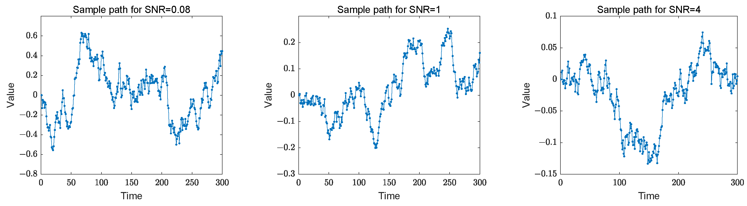The selection of these parameters is relevant to the results of the real data example. Meanwhile, the signal-to-noise ratio (SNR) serves as a guide, calculated as the variance of ${\eta }_t$ relative to ${\epsilon }_t$ (Ito et al. (2022) [12]). Consequently, three representative SNR values, {0.08, 1, 4}, are considered by adjusting the variance of the error term in the observation equation. These three sample paths of our model are plotted in Figure 1. We can see that the sample paths are non-stationary and that variation in the parameter combinations results in a change in the sample dispersion of the samples.

Figure 1. Sample paths for SNR = {0.08, 1, 4} with sample size $T=300$.

The performance of the parameter estimates derived from the two methods is assessed using the mean absolute deviation (MAD) and the mean squared error (MSE). Let ${\beta }_{t,m}$ represent the true values and ${\widehat{\beta }}_{t,m}$ represent the corresponding estimates. The sample means and the evaluation criteria are defined as:

$$\begin{array}{c}\overline{\beta }={\displaystyle \frac{1}{MT}}{\displaystyle \sum _{m=1}^M}{\displaystyle \sum _{t=1}^T}{\beta }_{t,m},\overline{\widehat{\beta }}={\displaystyle \frac{1}{MT}}{\displaystyle \sum _{m=1}^M\sum _{t=1}^T}{\widehat{\beta }}_{t,m},\\ \mathrm{MAD}={\displaystyle \frac{1}{MT}}{\displaystyle \sum _{m=1}^M\sum _{t=1}^T}|{\beta }_{t,m}-{\widehat{\beta }}_{t,m}|,\mathrm{MSE}={\displaystyle \frac{1}{MT}}{\displaystyle \sum _{m=1}^M\sum _{t=1}^T}{({\beta }_{t,m}-{\widehat{\beta }}_{t,m})}^2.\end{array}$$

(14)

The MAD compares each element of $\mathit{\beta }$ and can be interpreted as the median distance between the estimate and the true process, reflecting the level of similarity between $\mathit{\beta }$ and $\widehat{\mathit{\beta }}$. The non-stationary nature of the data generation process can sometimes lead to the occurrence of outliers. In our analysis, we focus on the means of the estimated parameters. The simulated results are summarized in Table 1 and Table 2. The estimators of ${\sigma }_{\epsilon }^2$ and ${\sigma }_{\eta }^2$, derived from Equation (9), are formulated as follows:

$$\begin{array}{cc}& {\widehat{\sigma }}_{\epsilon }^2={\displaystyle \frac{1}{MT}}{\displaystyle \sum _{m=1}^M\sum _{t=1}^T}{[y_{t,m}-\widehat{g}({\widehat{\beta }}_{t,m};{\widehat{\beta }}_{t,m})y_{t-1,m}]}^2,\hfill \\ & {\widehat{\sigma }}_{\eta }^2={\displaystyle \frac{1}{MT}}{\displaystyle \sum _{m=1}^M\sum _{t=1}^T}{({\widehat{\beta }}_{t,m}-{\widehat{\beta }}_{t-1,m})}^2,\hfill \end{array}$$

(15)

where $y_{t,m}$ represents the observation at time t, generated by each repetition. The simulation results are given in Table 3. As the sample size increases, the variance estimates asymptotically approach the true values, reflecting the consistency of the estimators.

Table 1. Simulation results for different settings; we report mean of true values ($\overline{\beta }$), mean of estimated parameters ($\overline{\widehat{\beta }}$), MAD, and MSE for OLS estimation.

${\mathit{\sigma }}_{\mathit{\epsilon }}^{\mathbf{2}}$	SNR	T	$\overline{\mathit{\beta }}$	$\overline{\widehat{\mathit{\beta }}}$	MAD	MSE
${0.07}^2$	0.08	100	−0.00170	−0.00264	0.11497	0.01997
		200	0.00026	0.00248	0.08160	0.01003
		300	0.00029	0.00169	0.06627	0.00667
${0.02}^2$	1	100	0.00272	0.00369	0.11423	0.01983
		200	−0.00259	−0.00299	0.08184	0.01008
		300	0.00160	0.00232	0.06695	0.00673
${0.01}^2$	4	100	0.00115	0.00328	0.11272	0.02003
		200	−0.00107	−0.00336	0.08114	0.00993
		300	0.00010	0.00274	0.06820	0.00690

Table 2. Simulation results for different settings; we report mean of true values ($\overline{\beta }$), mean of estimated parameters ($\overline{\widehat{\beta }}$), MAD, and MSE for Kalman-smoothing estimation.

${\mathit{\sigma }}_{\mathit{\epsilon }}^{\mathbf{2}}$	SNR	T	$\overline{\mathit{\beta }}$	$\overline{\widehat{\mathit{\beta }}}$	MAD	MSE
${0.07}^2$	0.08	100	0.00296	0.00157	0.11152	0.01912
		200	−0.00193	−0.00099	0.08011	0.00974
		300	−0.00105	−0.00254	0.06698	0.00674
${0.02}^2$	1	100	−0.00003	−0.00093	0.11334	0.01964
		200	0.00161	0.00099	0.08133	0.00992
		300	−0.00368	−0.00277	0.06587	0.00654
${0.01}^2$	4	100	0.00005	0.00348	0.11294	0.01954
		200	0.00287	0.00113	0.08119	0.00992
		300	0.00029	0.00069	0.06720	0.00675

Table 3. Simulation results for different settings; we report the OLS residuals.

	SNR = 0.08		SNR = 1		SNR = 4
$\mathit{T}$	${\widehat{\mathit{\sigma }}}_{\mathit{\epsilon }}^{\mathbf{2}}$	${\widehat{\mathit{\sigma }}}_{\mathit{\eta }}^{\mathbf{2}}$	${\widehat{\mathit{\sigma }}}_{\mathit{\epsilon }}^{\mathbf{2}}$	${\widehat{\mathit{\sigma }}}_{\mathit{\eta }}^{\mathbf{2}}$	${\widehat{\mathit{\sigma }}}_{\mathit{\epsilon }}^{\mathbf{2}}$	${\widehat{\mathit{\sigma }}}_{\mathit{\eta }}^{\mathbf{2}}$
100	0.00541	0.00030	0.00031	0.00034	0.00021	0.00036
200	0.00449	0.00034	0.00037	0.00037	0.00018	0.00039
300	0.00479	0.00038	0.00042	0.00038	0.00013	0.00039

Table 1 and Table 2 display some important statistical metrics for the estimators obtained by 1000 replications across various sample sizes. First, note that the order of magnitude of the MAD is much larger compared to the order of magnitude of $\overline{\beta }$. As shown in (14), the comparison between $\overline{\beta }$ and $\overline{\widehat{\beta }}$ is the mean of all the true and estimated values. Since the expectation of ${\beta }_t$ is 0, the overall means of the sample are all very close to 0. In contrast, the MAD compares each element of the true and estimated values at the corresponding time point. Also, the values of ${\beta }_{t,m}$ can be both positive and negative. As a result, they may cancel each other out when absolute values are not used. This, combined with the variability of ${\beta }_t$, explains why MAD exhibits a relatively large magnitude. Observing the trend, both the MAD and MSE decrease with an increase in sample size. This trend indicates that the precision of the OLS and Kalman-smoothing estimations improves as the sample size grows. Specifically, for smaller sample sizes (e.g., $T=100$), the estimation error is relatively large. However, as the sample size increases to $T=300$, the error metrics for both methods decrease significantly, indicating that larger sample sizes reduce estimation error and improve the predictive performance. Additionally, while varying parameter selections have a minimal impact on the estimation outcomes, it is evident that the impact on the two methods is different. OLS performs better at lower SNR values, as indicated by the smaller MAD and MSE in Table 1 for $T=300$. The Kalman-smoothing works relatively well when the SNR approaches 1. Furthermore, in the assessment of performance for nine different parameter settings, including various SNR and sample sizes T, based on the comparison of the 18 MAD and MSE values in Table 1 and Table 2, the OLS estimation performs better for 4 values, while the Kalman-smoothing estimation performs better for the remaining 14 values. But their differences are very small. In practice, the Kalman-smoothing estimation is observed to be more computationally efficient. Therefore, for models of this nature, the Kalman-smoothing estimation may be deemed more appropriate. Table 3 shows the behavior of the OLS residuals. As the sample size increases, the residuals get closer to the true values. This is an expected result since larger sample sizes typically have higher accuracy.

We calculate the mean of the estimation measures to focus on the overall performance of the methods. However, this approach does not allow us to verify the proximity of each estimated value ${\widehat{\beta }}_{t,n}$ to the true ${\beta }_{t,n}$ across the sample period. Moreover, as the sample size increases, the number of parameters to be estimated also grows, potentially introducing a significant bias in fitting the function $g(·)$. To address this, we fit the curves of $cos\left(\pi w\right)$ by substituting the true ${\beta }_{t,n}$ into the estimator $\widehat{g}(w;{\beta }_{t,n})$ from Equation (4). Due to the fact that there are as many estimators as observations T and the non-stationarity of the model, the asymptotic theories are not involved in the previous section. 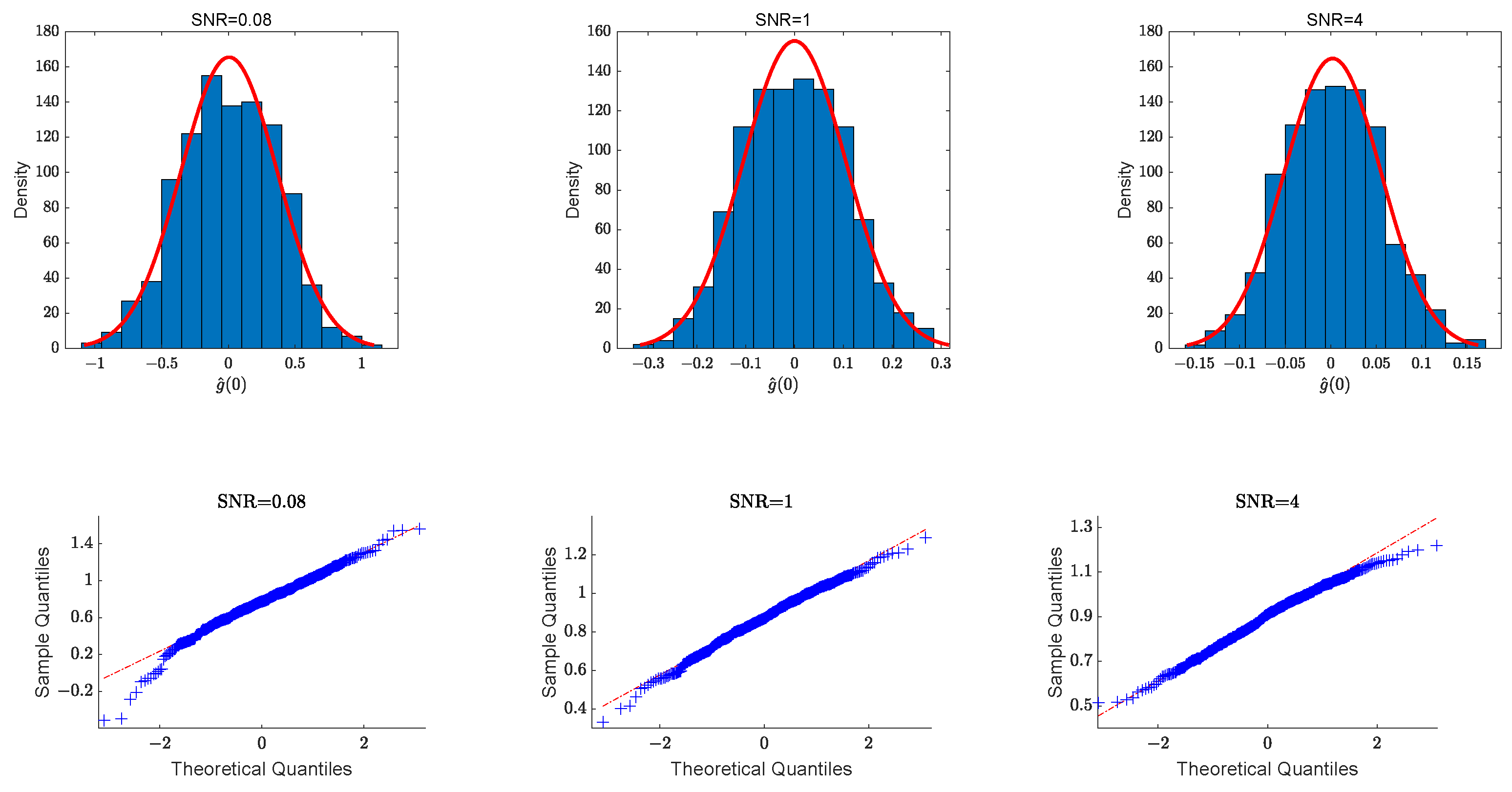However, the asymptotic nature of $\widehat{g}(·)$ is verified using histograms and Q-Q plots. Since the values of ${\beta }_t$ are near 0, Figure 2 shows the histograms and Q-Q plots of $\widehat{g}(·)$ at point 0 for three parameter selections when the sample size is $T=300$. We can see that the vertical bars and distribution curves in the histograms and the scatter and straight lines in the Q-Q plots are very close to each other, meaning that empirically the estimates of the unknown function are asymptotically normal. 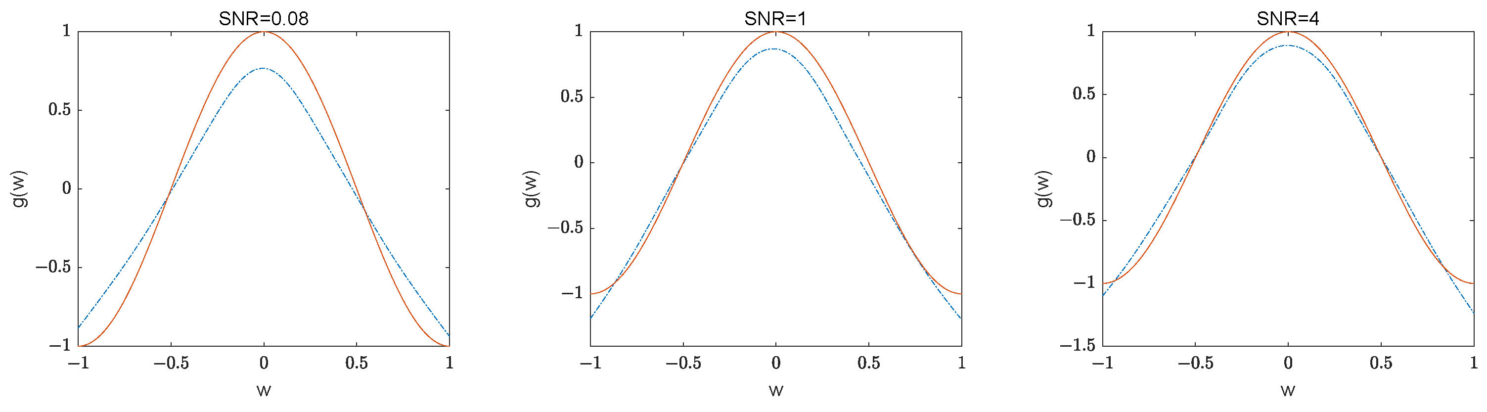Figure 3 presents the fitted curves of the function for SNR = {0.08, 1, 4} with sample size $T=300$. It is evident that the fitted curves are close to the real curves. The estimators for the unknown function $g(·)$ are assessed using the root mean squared error (RMSE), defined as RMSE = ${\left[{\displaystyle \frac{1}{T_{grid}}}{\displaystyle {\sum }_{t=1}^{T_{grid}}}{(\widehat{g}\left(w_t\right)-g\left(w_t\right))}^2\right]}^{1/2}$, where $\{w_t,t=1,\dots ,T_{grid}\}$ represent the regular grid points. Table 4 indicates that the RMSE values for $\widehat{g}(·)$ are small and decrease as the sample size increases.

Figure 2. The histograms and Q-Q plots of the $\widehat{g}\left(0\right)$ for the three parameter selections with sample size $T=300$. The red line in the histogram is the curve of normal density.

Figure 3. The real curve (red solid curve) and the fitted curve (blue dashed curve) of function $g\left(w\right)=cos\left(\pi w\right)$ when the sample size is $T=300$.

Table 4. Simulation results of RMSE for $\widehat{g}(·)$ under various SNR and sample sizes.

	SNR = 0.08			SNR = 1			SNR = 4
$\mathit{T}$	100	200	300	100	200	300	100	200	300
RMSE	0.4763	0.1924	0.1847	0.5247	0.1458	0.1086	0.5609	0.1483	0.0800

In summary, the simulation results substantiate the validity and effectiveness of the estimation methods used in this paper.

5. Real Data Example

This section utilized the closing points of the S&P/HKEX Large Cap Index (SPHKL) to demonstrate an application of our model and estimation methods. The dataset, spanning from 6 September 2020 to 28 January 2024, is accessible online at the website (https://cn.investing.com/indices/s-p-hkex-lc-chart, accessed on 11 February 2024). A stock index encapsulates the overall trend and volatility of stock prices in the market, making it a complex financial time series with characteristics such as time dependence, nonlinearity, and non-stationarity. Given these attributes, forecasting stock indices holds substantial practical importance for both investors and regulatory bodies. The dataset comprises 178 weekly observations, and Figure 4 illustrates their closing points along with the Partial Autocorrelation Function (PACF) plots. It is intuitively obvious from the sample path that the dataset is non-stationary.

Figure 4. Time plot and PACF plot of SPHKL closing points from 6 September 2020 to 28 January 2024.

We have also performed the Augmented Dickey–Fuller (ADF) test to examine the stationarity of the data. The results indicate the presence of unit root, with the p-value of 0.2172, suggesting that the dataset exhibits non-stationary behavior with a stochastic trend. The PACF plot corroborates this by revealing first-order autocorrelation, validating the suitability of our model for this dataset. The descriptive statistics for the data are displayed in Table 5. Its large variance implies that the data exhibit higher volatility and randomness, and the complexity of data interpretation also increases accordingly.

Table 5. Descriptive statistics for stock index data.

Sample Size	Minimum	Maximum	Median	Mean	Variance
178	20,559.76	48,702.22	30,917.10	32,965.24	47,385,547.70

For the analysis, the dataset is divided into a training set, encompassing 168 data points from 6 September 2020 to 19 November 2023 and a test set, comprising 10 data points from 26 November 2023 to 28 January 2024. The training set is used to fit the model and estimate the parameters, while the test set serves to evaluate the predictive ability of the model. The OLS method is used to estimate the parameters. The local linear regression method, as defined by $g({\widehat{\beta }}_t;{\widehat{\beta }}_t)$ in Equation (4), is used to estimate the function. 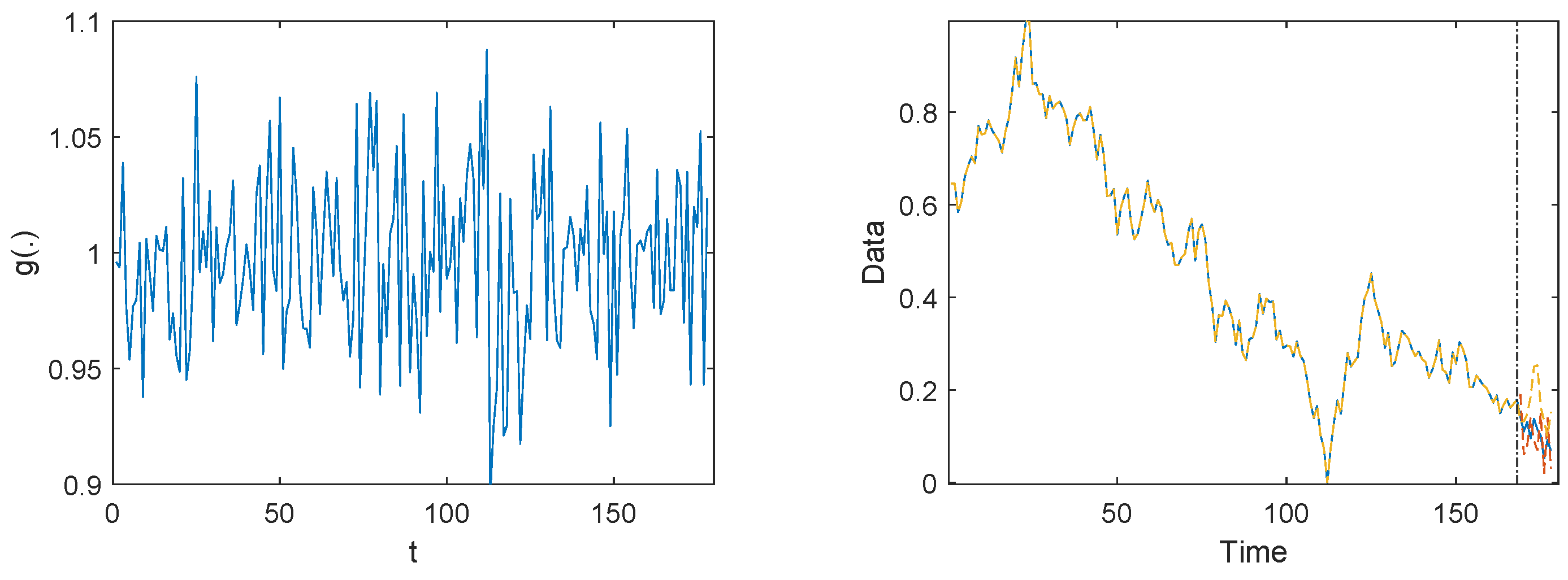The estimator of function $g(·)$ is presented in Figure 5. From the figure, we can see that there is a clear unsteady volatility. This volatility suggests that the model captures the dynamics in the time series data and that the autoregressive coefficient is not constant but varies over time. The estimated value of $\overline{\widehat{\beta }}$ is 0.0016, while the variances are estimated as ${\widehat{\sigma }}_{\epsilon }^2=0.00787$ and ${\widehat{\sigma }}_{\eta }^2=0.00005$.

Figure 5. The estimated function curve for t time points and sample path of the normalized data. The vertical line is used to distinguish between the training sample and the test sample. Shown to the right of the vertical line are blue for real data, red for forecast data using the proposed model, and yellow for forecast data using the RCA(1) model.

The h-step-ahead predictive values of the stock index data are formulated as follows:

$$E(y_{t+h}|y_t)=\prod _{k=1}^{h}g\left({\widehat{\beta }}_{t+k}\right)y_t.$$

The training set expands as more observations become available because ${\widehat{\beta }}_t$ changes with t. That is, for each additional prediction step, a further ${\beta }_t$ must be estimated. Because of the large order of magnitude of the sample data, the data are Min-Max Normalized $(y_t-min\left(y_t\right))/(max\left(y_t\right)-min\left(y_t\right))$ to eliminate the impact of the order of magnitude, allowing the data to be analyzed at the same scale. The descriptive statistics for the transformed data are displayed in Table 6. The sample path of the normalized data and the forecast data are presented in Figure 5. It is shown that the prediction on the test set seems to overestimate variability. This may be due to the complexity of our model, which could lead to overfitting. This overfitting may result in the model capturing noise in the training data rather than the underlying data-generating process, thereby inflating the estimated variability.

Table 6. Descriptive statistics for the normalized data.

Sample Size	Minimum	Maximum	Median	Mean	Variance
178	0	1	0.3680	0.4408	0.0598

The mean absolute deviation (MAD) and the root mean square error (RMSE) between the real stock index data and the predicted data are used to evaluate the predictive effectiveness of the model. Table 7 presents the results, comparing our model’s predictive performance with the RCA(1) model proposed by Nicholls and Quinn (1982) [1], which is defined as $y_t=(\alpha +B_t)y_{t-1}+{\epsilon }_t$, where $\alpha$ is a constant parameter, $B_t$ is a random term with mean zero and variance $\gamma$. The parameter estimates we obtained using the least squares method are $\widehat{\alpha }$ = 0.99207 and $\widehat{\gamma }$ = 0.05494. The data predicted by the RCA(1) model are also shown in Figure 5. A comparison of the prediction curves demonstrates that our model outperforms the RCA(1) model in predicting non-stationary data.

Table 7. The distance and error between forecasts and observations for stock index data.

Model	MAD	RMSE
Model (1)	0.0583	0.0642
RCA (1)	0.0678	0.0762

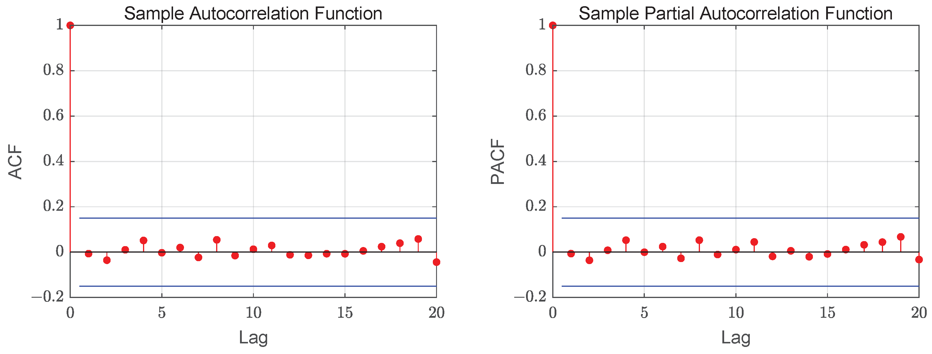
The results verify the performance of our model and method. To verify the adequacy of the model, we analyze the standardized Pearson residuals. Figure 6 exhibits the ACF and PACF plots of the residuals, which indicate the absence of correlation among the residuals. For our model, the mean and variance of the Pearson residuals are 0.0685 and 1.0003, respectively. As discussed in Aleksandrov and Wei (2019) [33], for an adequately chosen model, the variance of the residuals should take a value approximating 1. Accordingly, the proposed model is deemed to fit the data satisfactorily.

Figure 6. The ACF and PACF plots of the Pearson residual.

6. Conclusions

In recent years, despite advances in autoregressive models with random coefficients, research on nonlinear time series models driven by non-stationary state-space remains scarce. To address the intricacies of nonlinear and non-stationary characteristics, we introduce a novel random coefficient autoregressive model, incorporating an unobservable state variable. This model significantly enhances flexibility and efficiency in handling non-stationary data, particularly within the realms of economics and finance. To estimate the model’s unknown function and the parameters, we have developed methodologies using local linear regression, OLS, and Kalman smoothing. The analytical formulas for $\widehat{g}(·), {\widehat{g}}^{\prime }(·)$, $\widehat{\mathit{\beta }}$, ${\widehat{\sigma }}_{\epsilon }^2$, and ${\widehat{\sigma }}_{\eta }^2$ derived from these methods are presented. Numerical simulations demonstrate that our estimation approach is reliable, given a reasonably large sample size. When applied to a real data example, our model exhibits commendable performance. Additionally, our future research focuses on proving the asymptotic theory of estimators in non-stationary processes, while extending our findings to a higher-order AR(p) model represents a significant direction for advancing this field.