Enhancing Explainable Artificial Intelligence: Using Adaptive Feature Weight Genetic Explanation (AFWGE) with Pearson Correlation to Identify Crucial Feature Groups

Abstract

The ‘black box’ nature of machine learning (ML) approaches makes it challenging to understand how most artificial intelligence (AI) models make decisions. Explainable AI (XAI) aims to provide analytical techniques to understand the behavior of ML models. XAI utilizes counterfactual explanations that indicate how variations in input features lead to different outputs. However, existing methods must also highlight the importance of features to provide more actionable explanations that would aid in the identification of key drivers behind model decisions—and, hence, more reliable interpretations—ensuring better accuracy. The method we propose utilizes feature weights obtained through adaptive feature weight genetic explanation (AFWGE) with the Pearson correlation coefficient (PCC) to determine the most crucial group of features. The proposed method was tested on four real datasets with nine different classifiers for evaluation against a nonweighted counterfactual explanation method (CERTIFAI) and the original feature values’ correlation. The results show significant enhancements in accuracy, precision, recall, and F1 score for most datasets and classifiers; this indicates the superiority of the feature weights selected via AFWGE with the PCC over CERTIFAI and the original data values in determining the most important group of features. Focusing on important feature groups elaborates the behavior of AI models and enhances decision making, resulting in more reliable AI systems.

1. Introduction

The decision-making process of the majority of AI models is difficult to understand since they employ ‘black box’ machine learning (ML) methodologies. Users mostly find it hard to trust these systems due to their lack of clarity. Moreover, the inferences of intelligent models from instances cannot be monitored in detail because the training dataset is usually too large, and the learned model is too complicated for users [1]. As a result of these difficulties, researchers have become interested in explainable artificial intelligence (XAI). By offering analytical techniques to investigate and comprehend the behavior of the model, this field of research aims to validate important ML system properties that developers optimize, such as robustness, causality, usability, and trust. Explainable ML is concerned with providing post hoc explanations for existing black box models [2]. Explainability can answer explanatory questions such as ‘what’ questions (e.g., what event happened?), ‘how’ questions (e.g., how did that event happen?), and ‘why’ questions (e.g., why did that event happen?) [3].

A counterfactual explanation is a commonly used explanation approach that determines how the output changes by changing input features [4]. Simple explanations that are reflective of human cognition may be provided via counterfactual explanations, which can also encourage spontaneous causal reasoning about the result of a specific model [5]. Moreover, counterfactual explanations encourage analyzing the features of data instances and capturing the relationships between them and their impact on the outcomes [6]. Recent studies provide counterfactual explanations by perturbing input data to understand the limitations and biases of AI models and their training data rather than changing their predictions [7]. These explanations should change a few features, making them easy to understand and follow for end users, to improve human trust in AI models [8]. In fact, counterfactual explanations serve as significant mechanisms for assisting users in understanding automated systems and their decision-making processes. They emphasize that when the purpose of XAI is to enhance human–machine team performance, rather than just explaining model prediction, it is essential to study the user’s understanding of these decisions. For that, a more user-centered and psychologically grounded approach to XAI is required to study how explanations change the way users understand AI models [9].

For the AI model itself, providing counterfactual explanations highlighting the most important features as well as a group of features that affect the decision not only enhances the explainability of AI models for users but also boosts their performance. However, to the best of our knowledge, none of the proposed explanation techniques provide counterfactuals that include the importance of individual features or groups of features in the explanation. Our proposed method, thus, aims to bridge this gap by utilizing the feature weights from counterfactual explanations to identify the most crucial group of features that may have a significant impact on the decision-making process. Feature selection (FS) is one of the important steps in ML that keeps only the most meaningful group of features of a dataset while excluding others considered either irrelevant or redundant. This process enhances the performance of any ML model by increasing its accuracy, decreasing the complexity of the computational process, and reducing the amount of overfitting that might occur during training [10,11]. Some approaches that are frequently used for FS are correlation-based methods, which evaluate the associations between features in order to determine the most important groups of features. The Pearson correlation coefficient (PCC) is a widely used method for FS in ML learning, often integrated with other techniques, such as genetic algorithms (GAs), to enhance performance [12]. Therefore, in the current research, we used the PCC together with the feature weights obtained through adaptive feature weight genetic explanation (AFWGE) [13] to identify the most important group of features underlying a model’s decision. AFWGE is a novel technique that embeds feature weights while evolving and optimizing the counterfactual explanations, aiming to produce more accurate explanations than their nonweighted counterparts, as used in [14]. Therefore, it is intriguing to explore the potential of this technique in identifying the most important group of features that collectively have a significant impact on the decision-making process, which was the primary objective of this study.

The remaining parts of this paper are organized as follows: Section 2 provides an overview of related work, while Section 3 describes the formulation of the problem. Then, the proposed approach is explained in Section 4, followed by the provision of comprehensive experimental results in Section 5. Finally, Section 6 presents a summary and recommendations for future research.

2. Related Work

This section provides an overview of the most significant studies on counterfactual explanations and feature selection methods. The review focuses on foundational and recent works in these fields, highlighting their contributions and limitations. A summary of these works is presented in Table 1 for clarity and comparison.

2.1. Counterfactual Explanation

A counterfactual explanation is a post hoc explanation for potentially sophisticated black box models. These methods seek to explain how a fixed model leads to a particular prediction by perturbing variables to measure how the prediction changes. The counterfactual explanation describes the change to an input data point that would change a model’s prediction of it. Counterfactual explanations were proposed as a new approach in [15] to clarify automated choices, solving a number of concerns brought up by other studies regarding algorithmic interpretability and responsibility.

It was suggested [16] that an individual may modify a model’s decision by changing the feasible input variables. Multiple tests were conducted using an integer programming procedure for a credit scoring process. For data input, three real datasets, GiveMeCredit, German, and Credit [17], were utilized in each test. Differences were found in the difficulty of obtaining the given counterfactual condition across genders, indicating a substantial variation in the counterfactual generation cost. The authors of [14] presented a unified methodology to understand classification models and assess their robustness and fairness in the CERTIFAI tool. They used a unique GA to provide counterfactual explanations for the robustness, transparency, interpretability, and fairness of AI models. CERTIFAI was used in experiments to estimate the reliability of traditional classifiers such as decision trees (DTs), support vector machines (SVMs), and multilayer perceptron (MLP). Moreover, this tool was applied to assess the interpretability and fairness of such classifiers on the UCI Adult dataset. The study findings show how the proposed GA can give users convincing counterfactual explanations.

GeCo was introduced in [18] to seek optimal counterfactual explanations with the fewest modifications. GeCo also uses GAs to prioritize counterfactuals based on the number of modifications. The tests included a comparison of GeCo with five competitive tools, MACE [19], DiCE [20], WIT [21], CERTIFAI, and SimCF [22], using four real datasets. The datasets were Credit [17], Adult, Allstate, and Yelp. GeCo efficiently generated a plausible counterfactual explanation in a linear runtime that is almost as optimal as the ideal explanation in terms of distance. A new formulation of the optimization problem of counterfactual generation is presented in [23]. This formulation results in a single sparse counterfactual explanation that is efficiently produced through the normalization of continuous features and the selection of predictive features using a custom GA. The effectiveness of the proposed technique was assessed using credit-scoring datasets: German and Home Loan Equity. The assessment was based on a comparison of the generated counterfactual explanations with the provided explanations by credit-scoring specialists and the explanations of CERTIFAI [14] as a comparison. The results show that the presented method generates more sparse counterfactuals than CERTIFAI. In [6], a framework is proposed to adjust explanations based on user emotions, creating a more personalized, context-aware interaction with AI systems. By integrating emotional features, this approach aims to enhance user trust and satisfaction, making AI explanations more accessible and intuitive. This work underscores the need for a balance between factual accuracy and empathetic design in XAI, offering insights that align well with human-centered AI methodologies.

Most of the suggested explanation methods only estimate the importance of certain features using the model’s outcomes. After counterfactuals are generated, the importance of a feature is usually measured as the number of modifications of that feature in the generated counterfactuals [14]. With the exception of [13], none of the explanation methods manage to identify the importance of individual features or groups of features within the explanations themselves. On the contrary, the authors of [13] introduced an adaptive feature weight genetic explanation (AFWGE) method. This novel approach for generating counterfactual explanations uses GA with embedded feature weights as a reliable indicator of feature importance, providing valuable insights into understanding and interpreting the mechanisms underlying the model. By embedding feature weights as part of the counterfactual solution, AFWGE optimizes feature values and their weights alongside each other during the evolutionary process of the GA to generate more accurate counterfactual decisions. The empirical results on four datasets (Adult [24], Diagnostic Wisconsin Breast Cancer [25], Pima Indians Diabetes [26], and Iris [27]) show that AFWGE has significantly enhanced counterfactual generation performance, producing more efficient counterfactual explanations than CERTIFAI [14], which does not include feature weights in the counterfactual explanations. The results indicate that the counterfactual distances produced via AFWGE are significantly shorter than those of CERTIFAI. Similarly, the number of feature changes with AFWGE is significantly smaller than with CERTIFAI. Additionally, AFWGE changes features according to weights, demonstrating closer correlations to the dataset features’ correlations compared to the number of feature changes’ correlations exhibited by CERTIFAI. Moreover, AFWGE generates counterfactual explanations that fulfill fundamental properties: validity, proximity, sparsity, plausibility, and actionability of explanations.

2.2. Feature Selection (FS) Using the Pearson Correlation Coefficient (PCC)

One of the helpful phases in data modeling is feature selection, which aids in eliminating noisy, redundant, and irrelevant data. The goal is to create a predictive model with fewer input variables. It eliminates features from the model that might be redundant or useless predictors. Reducing the input features may lead to an improvement in the model’s performance in addition to lowering the computational cost of modeling. Additionally, we can increase the model’s generality by removing weak predictors [10].

A model may have its own features selected in many methods. Finding the most relevant and significant features may be accomplished by using the correlation between the features. Correlation-based feature selection (CFS) works well with higher-dimensional datasets. The CFS approach selects relevant features only based on the fundamental features of the data, without the use of algorithms for ML [28]. The features that are selected via the use of CFS yield a better level of accuracy in comparison to other methods [29]. In a dataset, it is common for some features to have a strong correlation with others. The presence of such strongly correlated features results in duplicate information that does not help enhance the model’s performance. The correlation among features is calculated using the CFS approach, and the highly correlated features, meaning they are similar, are not included [30]. Assuming that features p1 and p2 have a strong correlation, indicating that they contain similar types of information, a classification model that incorporates both p1 and p2 has an equivalent level of predictive capability to a dataset that includes either p1 or p2 individually.

A new FS method is introduced in [31], where a three-step process is used to reduce the number of features: First, remove redundant features using pairwise correlation. Then, let different methods select their own feature sets independently. After that, make sure that the individual feature sets have the same size. The individual feature sets are blended using both union and quorum procedures. Network anomaly detection was evaluated on both combined and individual sets with classifiers such as random forest (RF), DT, K-nearest neighbor (K-NN), Gaussian naïve Bayes, and logistic regression (LR). The experimental results on the UNSW-NB15 dataset indicated that the RF algorithm, when using both the union and quorum feature sets, achieved F1 scores of 99% and 99.02%, respectively.

The authors of [32] presented a gene FS technique that utilizes ReliefF [33] and a PCC algorithm. First, this technique uses ReliefF to evaluate the feature weight, then it sorts the features based on the weight and filters out genes that are not important based on a predetermined threshold. Next, any redundancies in the chosen feature subsets are removed using the PCC approach. To validate the proposed FS approach, three gene expression datasets were used for testing (Colon, Leukemia, and Prostate) with two classifiers, K-NN and SVM. In the experiment, the proposed approach achieved improved classification accuracy by successfully removing irrelevant and redundant genes.

The method introduced in [34] for selecting features consists of two stages. In the first step, the PCC is used to group features by finding the features that are correlated and then dividing them into groups based on how correlated they are (high, medium, or low). In the second step, the Triplet FS (TFS) method is introduced to prevent collinearity among features. This way, the features are selected based on the different correlations between each group. Lastly, the features in the triplet group are selected, and the LR approach is used to identify the disease. With an accuracy of 95.4%, an FPR of 1%, an FNR of 4%, a sensitivity of 97%, and a specificity of 96%, the classifier was able to differentiate between benign and malign types on the Breast Cancer dataset. Combining the PCC method with the TFS algorithm raised the accuracy, sensitivity, and specificity of breast cancer diagnosis. In [35], the authors focused on enhancing the accuracy of breast cancer diagnostics through machine learning techniques. The authors proposed a four-layered data exploration approach, including feature distribution analysis, correlation assessment, feature elimination, and hyperparameter optimization, to identify robust features for classifying tumors as malignant or benign. They developed and evaluated predictive models using the Wisconsin Diagnostic Breast Cancer (WDBC) and Breast Cancer Coimbra Dataset (BCCD). The results demonstrated that the polynomial SVM achieved 99.3% accuracy; LR, 98.06%; and KNN, 97.35% on the WDBC dataset, indicating the effectiveness of their approach.

The authors of [12] provided a hybrid FS method combining the PCC with a GA. The classifier decides whether someone has an illness by means of the acquired features as input. The chosen datasets—heart disease, diabetes, and hepatitis—were obtained from the UCI repository. The tests were intended to evaluate the performance of the GA and the PCC. The suggested approach had respective accuracies of 96.87%, 89.53%, and 97.03% on the hepatitis, diabetes, and heart disease datasets. The results revealed that the hybrid GA with PCC efficiently identifies relevant features, leading to superior accuracy for medical datasets. Another hybrid methodology introduced in [36], is an example of an approach to FS, namely, the ScC model. Stability (measuring how constant or stable the feature is) and correlation are employed as the criteria for eliminating data instances, specifically, instances with high stability and low correlation values. The suggested ScC model selects the most relevant features to maximize the accuracy of the classification. Four distinct classification algorithms were used to gauge the effectiveness of ScC. The performance of the proposed approach was evaluated using nine different benchmark datasets: Austra, Heart Disease, Phishing, Sonar, Iono, South-German-Credit, Spam-Base, Messidor, and Pop-Failure. Three state-of-the-art dimensionality-reduction methods were considered for comparison with the ScC method: PCA, rough set (RS), and weight-guided (WG). The results indicated that the ScC method reduces a given dataset with high predictive accuracy.

Two enhanced feature selection approaches using correlation and clustering are provided in [37]. In the correlation-based approach, feature correlation is used to determine a relationship type for each feature by selecting features based on a specific threshold. In the clustering-based version, the correlation data are analyzed using clustering to determine features that stand in for the whole cluster. The selected group of features of the two approaches was evaluated against the ReliefF feature selection approach by comparing the models’ performances. The two proposed approaches produced superior results, where their selected features increased the learning models’ accuracy.

The PCC is effective in eliminating redundant features and improving classification accuracy when combined with other methods such as ReliefF and GAs [12,32,34]. Of course, it has proven to have higher accuracy and provide better feature reduction when compared to conventional FS methods. More importantly, the PCC was successfully used with very good results for gene expression analysis [32], medical diagnosis [12], and network anomaly detection [31], proving its flexibility and efficiency.

The current study aimed to employ the feature weights obtained via the AFWGE method [13] with the commonly used PCC [29] to identify and manage redundancy among features. AFWGE is an approach for generating counterfactual explanations of AI models where a custom GA is employed, incorporating adaptive feature weights to enhance the algorithm’s performance. AFWGE makes use of experimentally determined feature weights. These weights take specific values in the algorithm, where they are equally initialized and then evolved adaptatively during the search. Consequently, search accuracy, exploration, exploitation, convergence speed, and overall algorithm behavior are guided by these adaptive weights. In fact, these weights have a significant impact on the behavior of the method since they are also optimized together with the main optimization of the counterfactual solution. In this current study, we advanced AFWGE by integrating the feature weights generated by AFWGE with the commonly used PCC to manage feature redundancy effectively. Here, the feature weights computed by AFWGE serve as a reliable indicator of feature importance, guiding the PCC computations to evaluate the correlations among features and identify the most crucial feature groups. This approach not only reduces redundancy but also enhances the interpretability, providing deeper insights into the underlying mechanisms of the AI model.

The weights for the features computed via AFWGE guide the computations of the PCC efficiently for evaluating the correlations between features and identifying the most crucial group of features. Thus, highly correlated feature weights are finally reduced to one feature. This ensures that the finally obtained set of features is nonredundant and contains the most influential ones that increase the efficiency of the learning model to avoid overfitting. Incorporating feature weights with the PCC provides a finer and more effective process for FS, which eventually improves model performance and explainability. Interestingly, this study highlights the role of AFWGE feature weights as reliable indicators of feature importance, providing valuable insights into understanding and interpreting the underlying mechanisms of the model.

Table 1. Summary of the literature review.

	Method	Model	Property
Counterfactual Explanation	Integer programming	LR	Produce flip-sets	[16]
	GA	DT, SVM, MLP	Assess interpretability	[14]
	GA	MLP	Real-time performance	[18]
	GA	RF, artificial neural networks	Select predictive features using RF	[23]
	Emotion lexicons	Large language models	Emotional features for human-centered AI	[6]
	GA	MLP	Feature weights obtained through adaptive feature weight genetic explanation	[13]
Features Selection	Ensemble learning	RF, DT, K-NN, Gaussian naïve Bayes, LR	Union and quorum procedures	[31]
	PCC and ReliefF	K-NN, SVM	Removing irrelevant and redundant genes	[32]
	PCC and TFS	LR	Lowering the number of false positive and false negative reports	[34]
	4-layered data exploration	SVM, LR, KNN	Improving diagnostic accuracy	[35]
	PCC and GA	K-NN	Hybrid GA with PCC efficiently identifies relevant features	[12]
	Stability and correlation	LR, fast and large margin, RF, gradient-boosted trees	Pick optimal reduction with high stability and low correlation	[36]
	Correlation and clustering	LR, artificial neural networks	Superior to ReliefF	[37]

Table 1. Summary of the literature review.

	Method	Model	Property
Counterfactual Explanation	Integer programming	LR	Produce flip-sets	[16]
	GA	DT, SVM, MLP	Assess interpretability	[14]
	GA	MLP	Real-time performance	[18]
	GA	RF, artificial neural networks	Select predictive features using RF	[23]
	Emotion lexicons	Large language models	Emotional features for human-centered AI	[6]
	GA	MLP	Feature weights obtained through adaptive feature weight genetic explanation	[13]
Features Selection	Ensemble learning	RF, DT, K-NN, Gaussian naïve Bayes, LR	Union and quorum procedures	[31]
	PCC and ReliefF	K-NN, SVM	Removing irrelevant and redundant genes	[32]
	PCC and TFS	LR	Lowering the number of false positive and false negative reports	[34]
	4-layered data exploration	SVM, LR, KNN	Improving diagnostic accuracy	[35]
	PCC and GA	K-NN	Hybrid GA with PCC efficiently identifies relevant features	[12]
	Stability and correlation	LR, fast and large margin, RF, gradient-boosted trees	Pick optimal reduction with high stability and low correlation	[36]
	Correlation and clustering	LR, artificial neural networks	Superior to ReliefF	[37]

3. Problem Formulation

The feature selection problem is concerned with finding the best subgroup of features from a dataset to train the learning model, where this subgroup improves performance compared with using all features or at least provides the same performance as using all features, which can be mathematically described as follows:

Let $\mathsf{{\rm X}}\in {\mathbb{R}}^{n\times p}$ be the dataset with n samples and p features, and let $\mathrm{y}\in {\mathbb{R}}^n$ be the target variable. Define $\mathcal{F}=\{1, 2, \dots , p\}$ as the set of all features. We want to select a subgroup $S\subseteq \mathcal{F}$ that optimizes the performance of the learning model. Let ${\mathsf{{\rm X}}}_s$ denote the subset of $\mathsf{{\rm X}}$ containing only the features in $S$. Let $\mathcal{L}({\mathsf{{\rm X}}}_s,\mathrm{y})$ be the performance metric (e.g., accuracy, precision, recall, and F1 score) of the learning model trained on ${\mathsf{{\rm X}}}_s$ and evaluated on $\mathrm{y}$. The feature selection problem can be formulated as an optimization problem [38]:

$$\underset{S\subseteq \mathcal{F}}{\max }\mathcal{L}\left({\mathsf{{\rm X}}}_s,\mathrm{y}\right)$$

(1)

$$\mathrm{s}\mathrm{u}\mathrm{b}\mathrm{j}\mathrm{e}\mathrm{c}\mathrm{t} \mathrm{t}\mathrm{o} \mathcal{L}\left({\mathsf{{\rm X}}}_s,\mathrm{y}\right)\ge \mathcal{L}\left(\mathsf{{\rm X}},\mathrm{y}\right)-ϵ$$

(2)

where $\mathsf{ϵ}\ge 0$ is a small tolerance value that allows subgroup $S$ to perform slightly worse than using all features $\mathcal{F}$. This formulation seeks the subset $S$ that maximizes the performance of the learning model with a guarantee that it is at least as good as when using all features within tolerance $\mathsf{ϵ}$.

Subgroup $S$ must contain the features most relevant to the prediction problem that are not redundant. Feature $f_i$ is relevant if a change in the feature’s value results in a change in the value of the predicted class variable $C$. Feature $f_i$ is strongly relevant if the use of $f_i$ in the predictive model eliminates the ambiguity in the classification of instances. Feature $f_i$ is weakly relevant if $f_i$ becomes strongly relevant when a subset of the features is removed from the set of available features. This implies that a feature is irrelevant if it is not strongly relevant, and it is not weakly relevant [39]. For redundancy, feature $f_i$ is redundant relative to class variable $C$ and a second feature $f_j$ if $f_i$ has stronger predictive power for $f_j$ than for the class variable $C$ [40]. However, to make feature selection decisions, several researchers have explained a redundant feature as one that has a high correlation with all the other features [41].

4. Proposed Method

To optimize the feature selection and identify the most important group of features, we compute the PCC of the feature weights that are produced via the adaptive feature weight genetic explanation (AFWGE) in the generated counterfactuals, as explained in detail in [13]. AFWGE is a method that extends the standard GA with adaptive feature weights, allowing for improved counterfactual explanations. For a standard GA, the approach considers a normal population of random solutions, usually called chromosomes. Every chromosome represents one potential solution to the problem under study. The solutions are iteratively updated based on which operations, such as selection, crossover, and mutation, are applied, with the goal of optimizing a fitness function. It is an iterative process that repeats until some termination condition is met, such as when a certain number of generations is reached. AFWGE follows this structure but introduces adaptive feature weights that evolve together with counterfactual solutions.

AFWGE aims to analyze the explainability of a predictive model given the model as a black box model and the data instances. First, AFWGE initializes the population of chromosomes, with each chromosome composed of two parts: the feature values and the weights assigned to those features (Figure 1). The feature weights are initialized uniformly and adaptively evolve throughout the search process with the purpose of influencing the algorithm’s behavior. After that, the rating process based on an objective function is realized; in this sense, it is assumed that those solutions are ranked as better if they produce a minimal distance concerning the original instance. This is followed by the selection step, where a subset of the fittest within the population is selected for crossover. During the crossover phase, a number of pairs of chromosomes exchange feature values over selected features and create offspring. After that, mutation is applied to the offspring after crossover. In this stage, feature values and weights are both mutated. This population is then filtered out after mutation in order to remove all the chromosomes returning the same prediction as the original instance. This ensures that only those chromosomes whose predictions differ from the ones of the original instance remain in the population, while the algorithm focuses on the construction of valid counterfactual explanations. The process iterates until it meets a stop condition, such as when the best fitness score has not improved over five generations. Finally, AFWGE provides a list of the counterfactual explanations with the final feature weights. The analysis highlights the role of feature weights as reliable indicators of feature importance, providing valuable insights for understanding and interpreting the mechanisms underlying the model.

Figure 1. AFWGE flowchart.

Therefore, when given a black box predictive model and dataset as inputs to the AFWGE method, this produces superior counterfactual explanations with the weights of the final features (Figure 2). Then, these feature weights are used as the input and combined with correlation-based redundancy reduction, where the correlation between the features is computed using the PCC [42] to obtain the most crucial group of features. This technique calculates the linear relationship between each of the two features’ weights, thus detecting possible redundancy. If two features are found to have high absolute PCC values with each other, then we retain the one that has lower absolute PCC values with the other features and eliminate the other. The PCC is represented by Equation (3):

$$\rho \left(X,Y\right)={\displaystyle \frac{cov(X,Y)}{\sigma X\sigma Y}}={\displaystyle \frac{E\left[\left(X-\mu x\right)\left(Y-\mu y\right)\right]}{\sigma X\sigma Y}}$$

(3)

Figure 2. Process flow diagram of the proposed method.

The PCC, computed using Equation (3), is used to assess the linear correlation between two variables, X and Y. The function cov(X, Y) is the covariance of X and Y. σX and σY are the deviations of X and Y, respectively; μx and μy are the respective means; and E is the expected value.

We can obtain a formula for ρ(X,Y) by substituting the estimates of the covariances and variances based on a sample input into the formula above. Given paired data {(x₁,y₁), (x₂,y₂), …, (x_n,y_n)}, consisting of n pairs, ρ(X,Y) is defined as per Equation (4), where n is sample size, x_i, y_i are the individual sample points indexed with i, and $\overline{x}$ and $\overline{y}$ are the sample means of variables X and Y, respectively.

$$\rho \left(X,Y\right)={\displaystyle \frac{{\sum }_{i=1}^n(x_i-\overline{x})(y_i-\overline{y})}{\sqrt{{\sum }_{i=1}^n{y_1(x_i-\overline{x})}^2}\sqrt{{\sum }_{i=1 }^n{(y_i-\overline{y})}^2}}}$$

(4)

ρ(X,Y) ranges from + 1 to −1, where a value of + 1 indicates that X is completely positively linearly correlated to Y. Conversely, a value of 0 signifies that X is not linearly correlated to Y at all. Finally, a value of −1 indicates that X is completely negatively linearly correlated to Y. X and Y are typically considered to exhibit an extremely strong correlation with each other when ρ(X,Y) is greater than 0.8. Moreover, X and Y exhibit a strong correlation to each other when ρ(X,Y) is greater than 0.6 [43].

5. Computational Experiments

We empirically tested the usefulness of our proposed method for users, model developers, and regulators in two steps: first, training and testing the classifier with original Data (having all the features); second, training and testing the classifier with the updated dataset that had the set of crucial features alone, obtained via our proposed method. In the following subsections, we explain all the details concerning the experimental setup and the implementation environment used to test our approach, followed by all the details of the results obtained.

5.1. Experimental Setup

5.1.1. Datasets

We took the same four real datasets used in AFWGE [13] and CERTIFAI [14]: (1) the Adult dataset [24], used to predict whether the income of an adult exceeds 5000 USD/year using U.S. census data from 1994; (2) the Diagnostic Wisconsin Breast Cancer dataset [25] to diagnose whether a breast tumor is malignant or benign; (3) Pima Indians Diabetes [26] to predict whether or not a patient has diabetes, based on certain diagnostic measurements, where all patients are women at least 21 years old and of Pima Indian heritage; and (4) the Iris dataset [27] to predict the type of the Iris plant from three types. Table 2 provides the details of the dataset considered for the experiments.

Table 2. Characteristics of the datasets.

	Adult	Breast Cancer	Pima Indians Diabetes	Iris
Dataset Size	48,842	569	768	150
Sample Size	30,163	569	768	150
Number of Features	14	30	8	4
Outcome Classes	2	2	2	3
Dataset Size	48,842	569	768	150

5.1.2. Rival Methods

The aim of the experiments was to select the most important group of features underlying a counterfactual explanation by computing the PCC for the feature weights from AFWGE and then finding the most important group of features, as explained in Section 4. After that, the dataset was updated by taking the important group features that were obtained and excluding the rest. Next, we trained and tested the classifier on the updated dataset.

As previously motioned, both CERTIFAI and AFWGE use custom GAs. However, the main difference between them is that AFWGE assesses feature importance by incorporating feature weights as part of the solution and dynamically evolves them alongside feature values throughout the evolutionary process, while CERTIFAI assesses feature importance by computing the number of feature changes in the produced counterfactual explanations. Therefore, for each dataset, we compared each classifier’s performance using three different feature groups:

• Original data feature groups: The important group of features identified using the PCC for feature values from Original Data;
• AFWGE feature groups: The important group of features identified using the PCC for the feature weights produced via AFWGE [13];
• CERTIFAI feature groups: The important group of features identified using the PCC for the number of feature changes, as produced via CERTIFAI [14].

5.1.3. Evaluation Metrics

To measure the performance of each classifier, we used the following widely accepted performance statistics: accuracy, precision, recall, and F1 score.

5.1.4. The Classification Models

We chose nine ML classifiers to evaluate the same four datasets: Adult, Breast Cancer, Pima Indians Diabetes, and Iris. These included three simple learners: LR, linear and radial SVM (L-SVM and R-SVM), and DT and ensemble learners (RF, which uses a set of homogenous DTs as its base classifiers). Additionally, we used AdaBoost, K-NN, Gradient Boosting, and MLP.

5.1.5. Setup

We used the scikit-learn library within the Python implementation environment on macOS. The classifier parameters were left as the default by the scikit-learn library. All datasets were evaluated with the same model configurations. To obtain the feature weights selected via AFWGE and the number of features changes of CERTIFAI, we reimplemented AFWGE and CERTIFAI in Python 3.10 on MAC studio Apple (Cupertino, CA, USA) M1 Ultra with 128 GB RAM on the same four real datasets used in AFWGE and CERTIFAI with the same parameters as in [13]. We implemented all three methods for finding the most important group of features, using either AFWGE, CERTIFAI, or Original Data in Python 3.10. All experiments were run on a MAC 1.4 GHz Quad-Core Intel Core i5 with 8 GB RAM. For the PCC threshold, we applied multiple tests with values equal to 0.6, 0.7, 0.8, 0.9, 0.95, and 0.99. These threshold values were chosen to systematically evaluate the impact of varying levels of correlation on feature reduction. These values provided a balanced range from high to extremely high correlation, allowing us to explore the trade-off between feature redundancy and model interpretability. Studies aiming to improve model performance also indicated better results with a PCC threshold of 0.6 or higher, which is a commonly used threshold in feature selection studies [44]. While these thresholds performed well across the datasets used in this study, their applicability may vary depending on the dataset characteristics, such as feature dimensionality and the degree of correlation among features. However, selecting an optimal threshold for a dataset may require more analysis to understand its correlation structure.

5.2. Experimental Results

This section presents the outcomes of training and testing the classifiers using the three different methods for calculating the most important group of features and comparing them according to the aforementioned evaluation criteria. First, we present the PCC results of each method. Then, we assess and compare the classifier metrics, each in a separate subsection: accuracy, precision (Appendix A), recall (Appendix B), and F1 score. Next, we provide an extensive evaluation of the proposed method’s performance. Finally, we provide insights into the relationship between the collective importance of feature groups and the importance of individual features.

5.2.1. PCC Results

Examining the heatmaps of the Pearson correlation coefficients for the Adult, Breast Cancer, Pima Indians Diabetes, and Iris datasets was crucial for understanding the relationships between features in each dataset. These heatmaps are visual representations of the strength and direction of the linear relationship between two features. These give insights into the relevance of features and possible redundancies. Moreover, the heatmaps demonstrate how the different inputs used to compute the PCC for each method can impact the correlation values for each dataset, as shown next. This comparison highlights how the AFWGE feature weights serve as indicators of feature correlations compared to the number of feature changes in CERTIFAI and the original feature values.

• Adult:

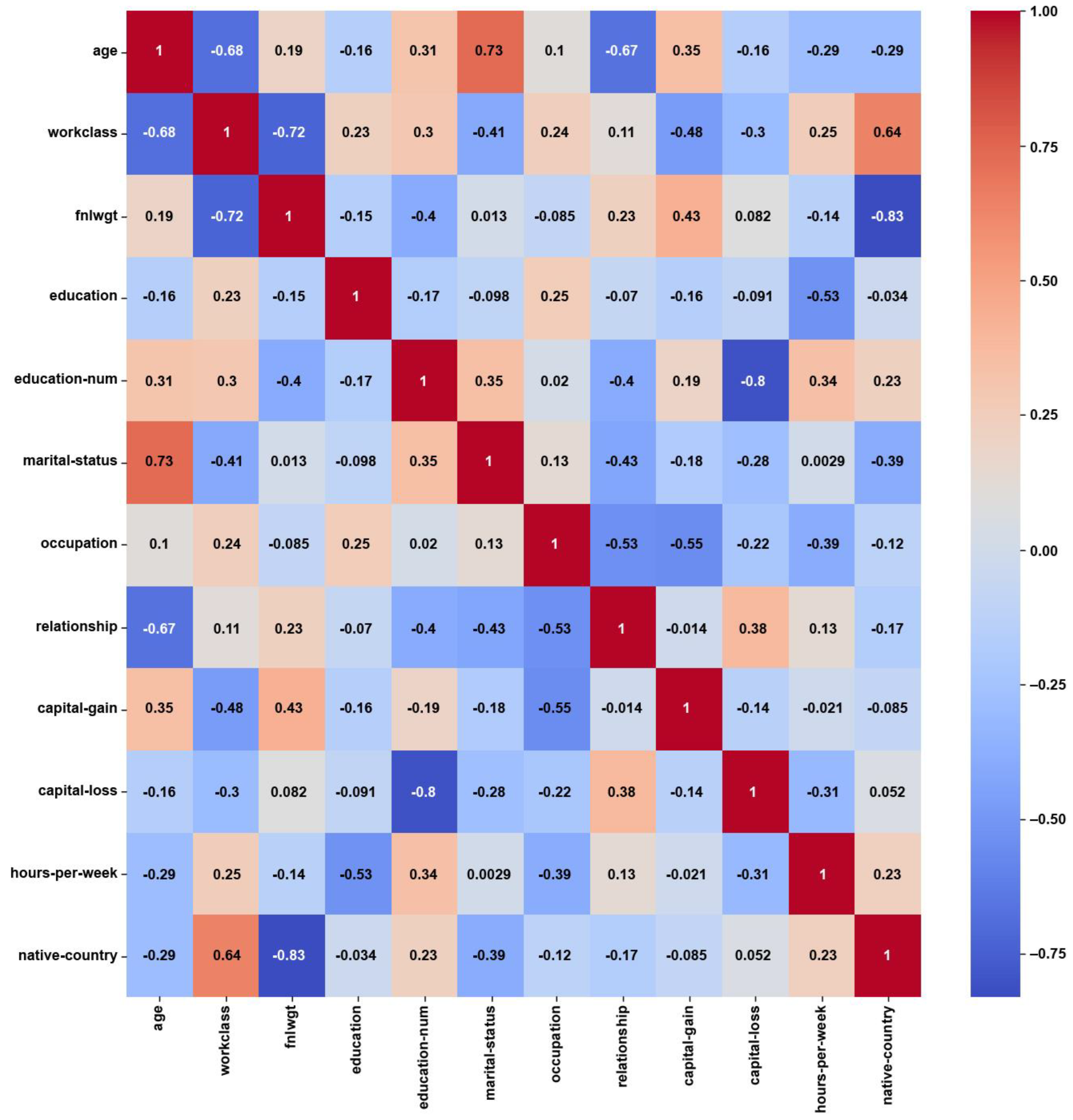
For the Adult dataset, the heatmap in Figure 3 shows weak correlations, with maximum PCC values of around ±0.3, which might have been caused by the notable class imbalance. About 75% of the instances belong to the ‘income ≤ 50 K’ class, while the remaining 25% belong to the ‘income > 50 K’ class. On the other hand, the feature weights by AFWGE (Figure 4) and the number of feature changes by CERTIFAI (Figure 5) show higher correlations, with maximum PCC values of around ±0.8 and ±0.7, respectively. These high correlations are not due to the unified numerical type of features (i.e., the weights by AFWGE or the number of changes by CERTIFAI); rather, the weights of the features by AFWGE and the number of feature changes by CERTIFAI seem to provide more efficient encoding of categorical features and expressing all features, in general, to interpret correlations accurately.

Figure 3. Adult heatmap of Original Data PCC using feature values from Original Data.

Figure 4. Adult heatmap of AFWGE PCC using the feature weights produced by AFWGE.

Figure 5. Adult heatmap of CERTIFAI PCC using the number of feature changes produced by CERTIFAI.

• Breast Cancer:

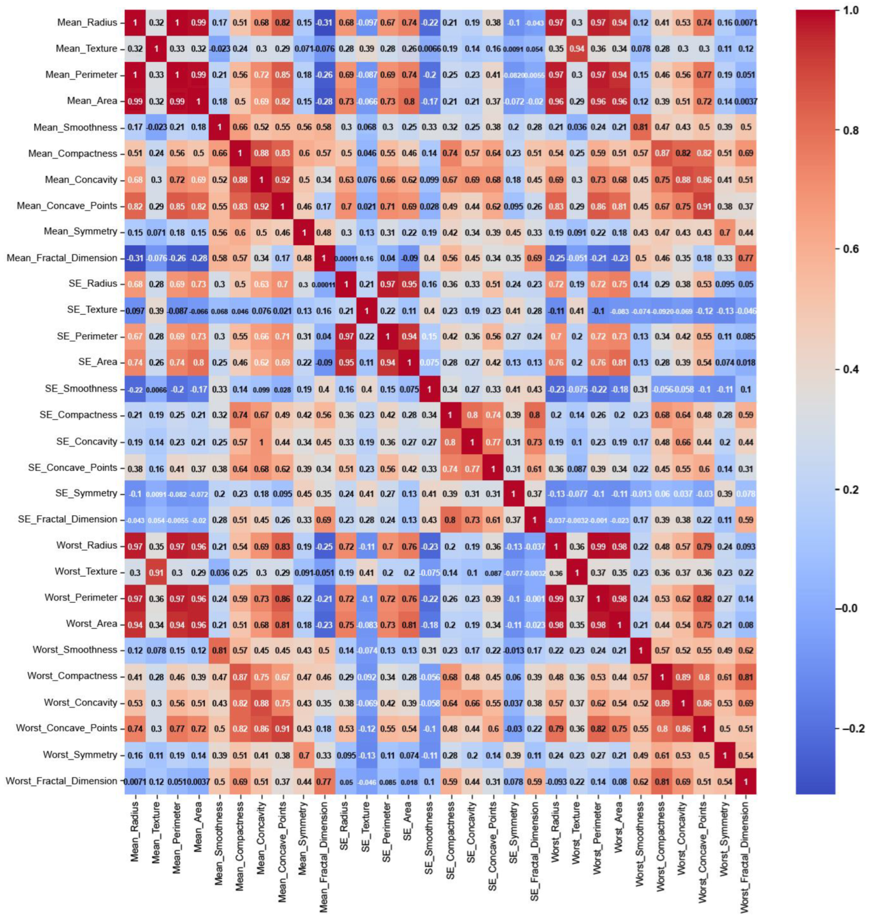
This dataset is balanced with two classes (malignant and benign), consisting entirely of numerical features related to medical measurements, and is likely to show stronger and more meaningful correlations. The heatmap of the Original Data PCC using the feature values from the Breast Cancer dataset in Figure 6 shows strong correlations, with maximum PCC values of around 0.9 and PCC values of at least 0.7 for most features; it represents 21% of all feature correlation pairs (92 pairs out of 435). Ambiguity is introduced by the high correlations among the features since feature selection methods might struggle to distinguish which feature to keep when multiple features are highly correlated. 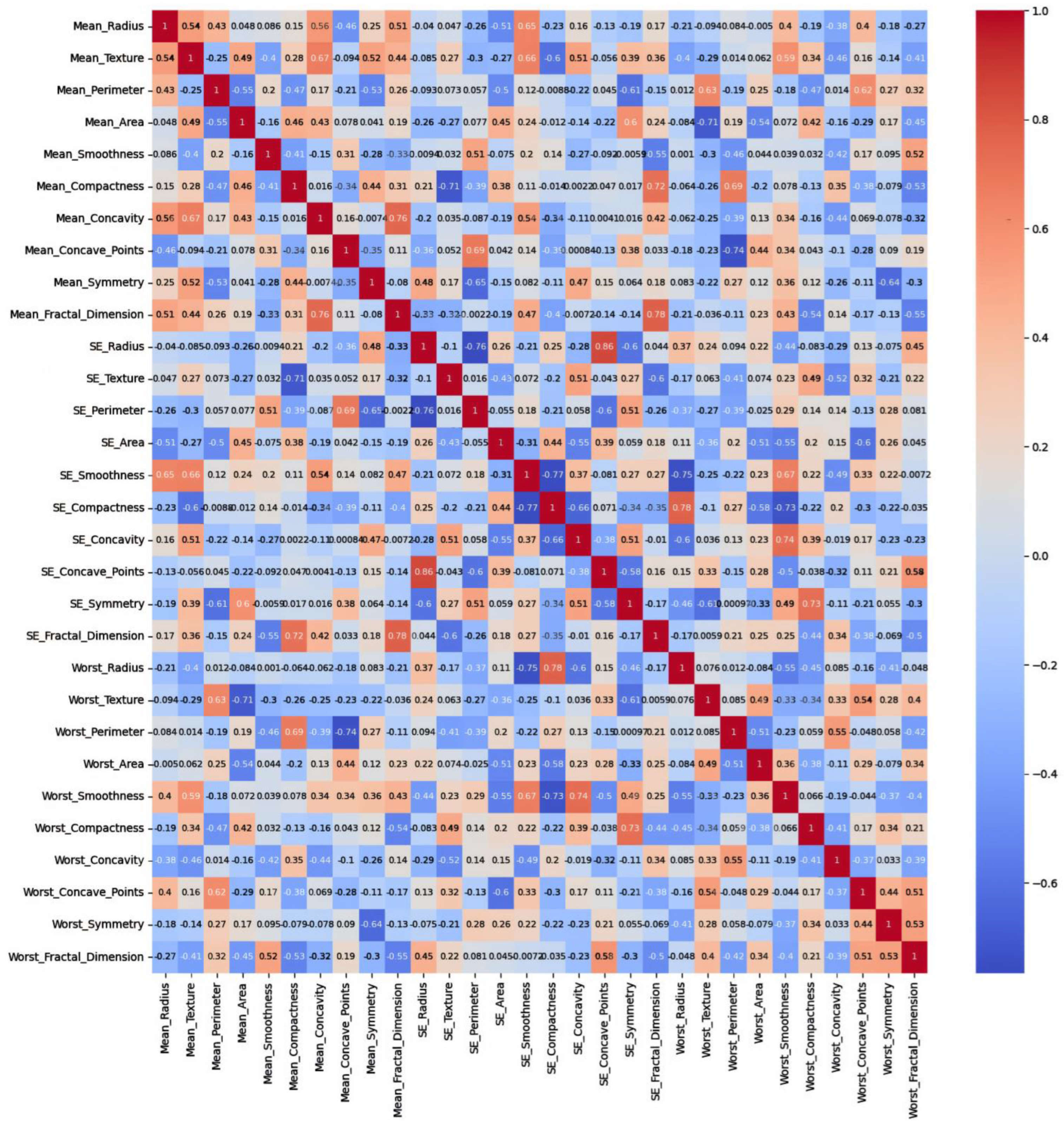This can lead to uncertain decisions about which features are truly significant, potentially leading to the exclusion of valuable features or the inclusion of redundant ones [37]. On the other hand, the feature weights of AFWGE (Figure 7) and the number of feature changes of CERTIFAI (Figure 8) show how these high correlations are filtered by eliminating a number of them. Feature correlation pairs with PCC values of at least 0.7 were eliminated by AFWGE (15 pairs out of 435) and CERTIFAI (20 pairs out of 435). This filtration prevents ambiguity in the feature selection process.

Figure 6. Breast Cancer heatmap of Original Data PCC using feature values from Original Data.

Figure 7. Breast Cancer heatmap of AFWGE PCC using the feature weights produced by AFWGE.

Figure 8. Breast Cancer heatmap of CERTIFAI PCC using the number of feature changes produced by CERTIFAI.

• Pima Indians Diabetes:

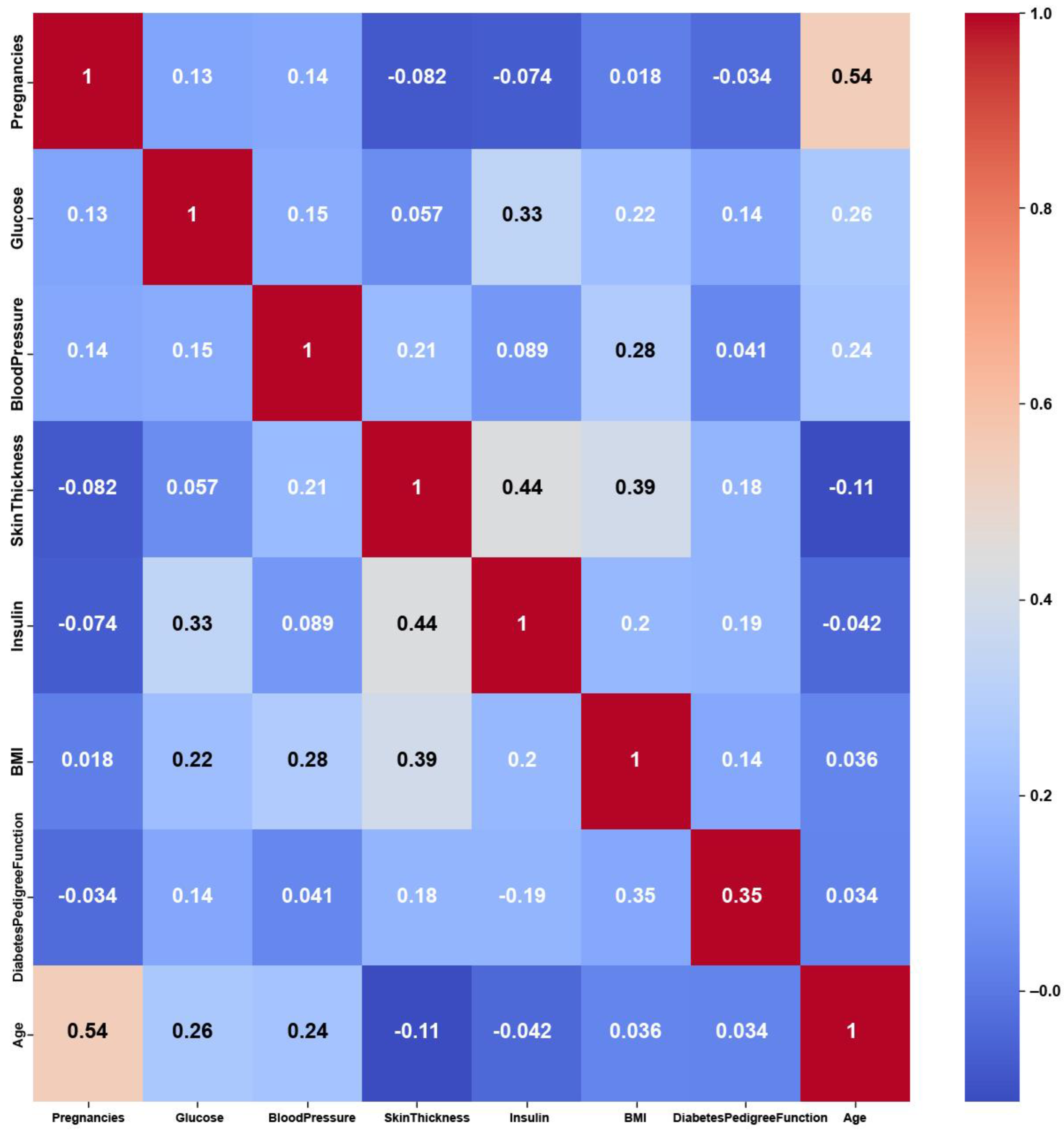
The Pima Indians Diabetes dataset consists of numerical features, yet it shows weak correlations among these features, as shown in Figure 9, with maximum PCC values of around 0.5. The weak correlations might have been due to dataset imbalance, with 35% labeled as diabetic and 65% of the instances labeled as nondiabetic. Nevertheless, the features might not be strongly correlated with each other, but they are still relevant for predicting diabetes. On the other hand, the feature weights of AFWGE (Figure 10) and the number of feature changes of CERTIFAI (Figure 11) show higher correlations than Original Data. However, they still do not have strong PCC values, i.e., not exceeding 0.6 for either AFWGE or CERTIFAI.

Figure 9. Pima Indians Diabetes heatmap of Original Data PCC using feature values from Original Data.

Figure 10. Pima Indians Diabetes heatmap of AFWGE PCC using the feature weights produced by AFWGE.

Figure 11. Pima Indians Diabetes heatmap of CERTIFAI PCC using the number of feature changes produced by CERTIFAI.

• Iris

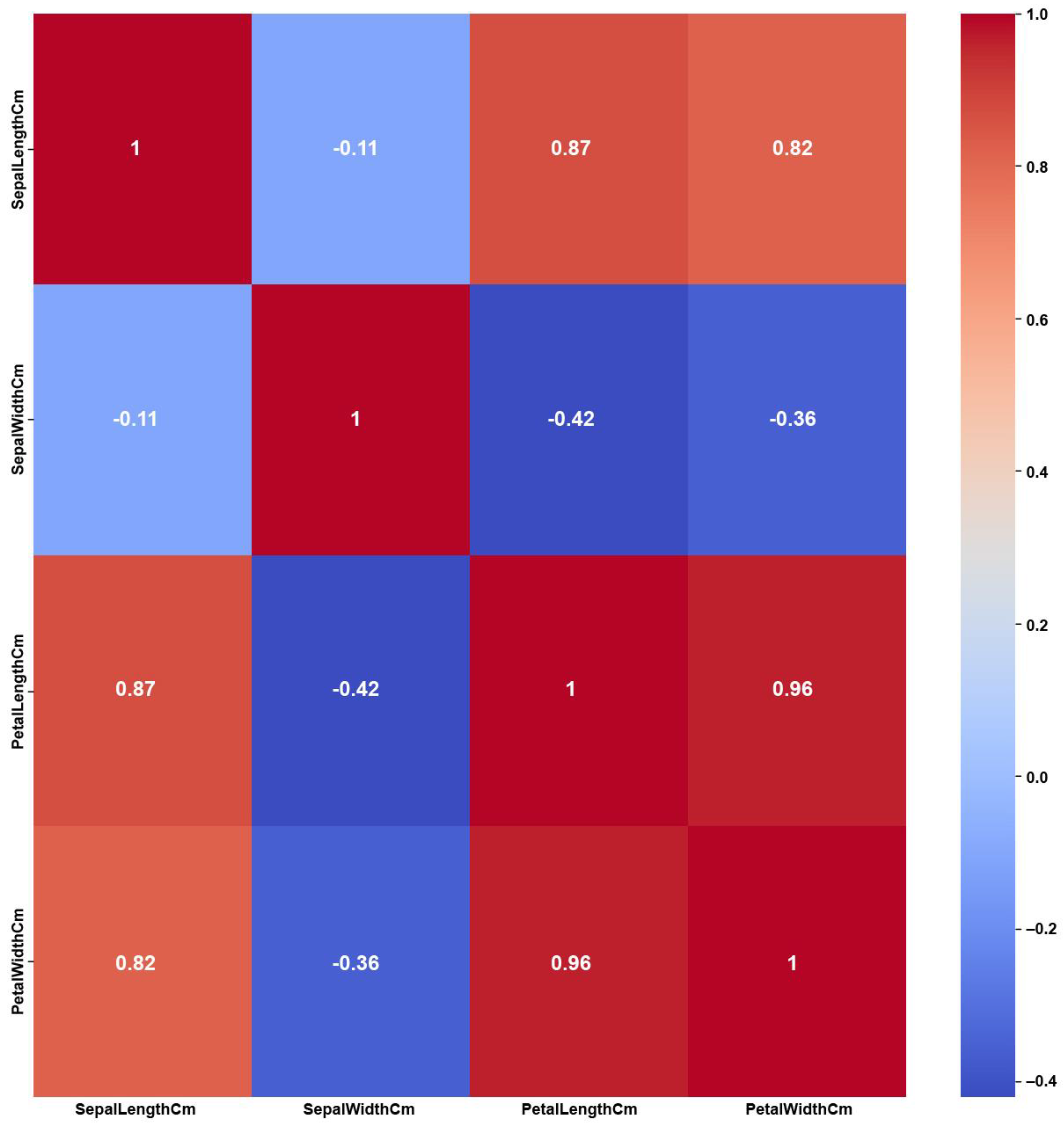
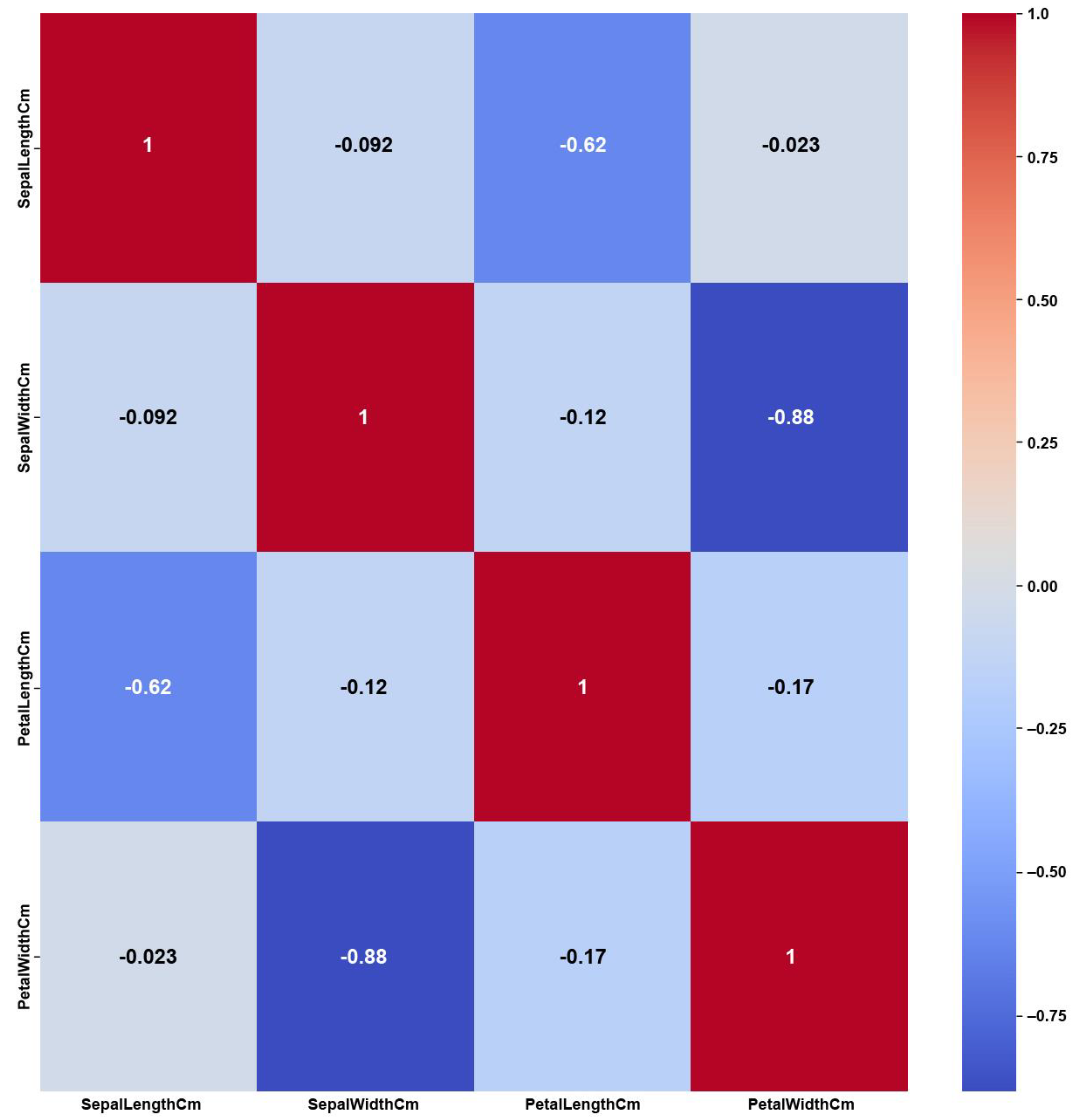
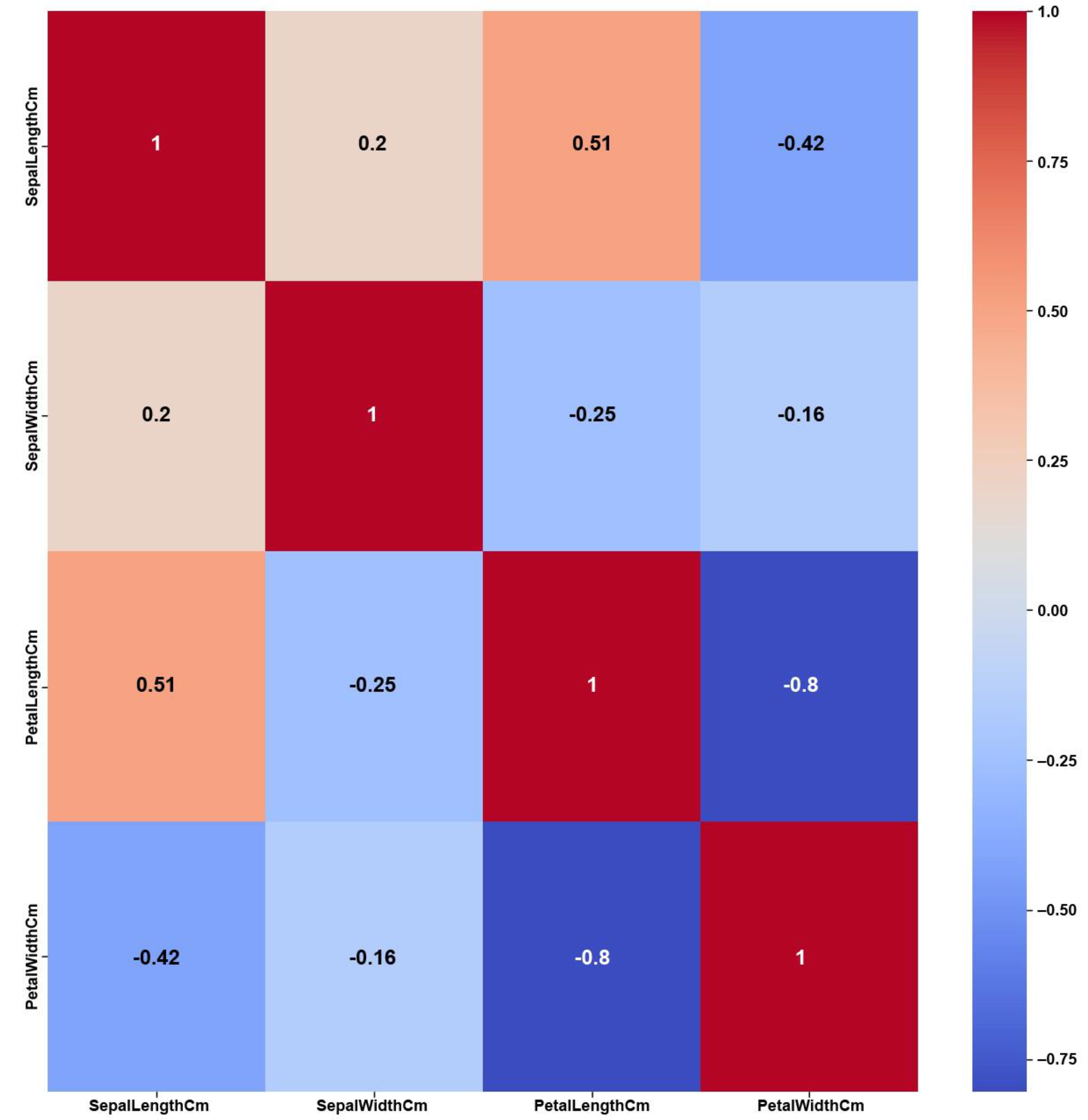
The Iris dataset’s simplicity, having a small number of features and balanced classes, shows clear and strong correlations among the features, as shown in the Original Data heatmap (Figure 12). The figure shows a maximum PCC value of around 0.9 and PCC values of at least 0.8 for most of the features, i.e., 50% of all feature correlation pairs (three pairs out of six). Again, as previously discussed in the Breast Cancer case, this high amount of feature correlations can lead to ambiguous decisions in feature selection. However, the feature weights of AFWGE (Figure 13) and the number of feature changes by CERTIFAI (Figure 14) show how these high correlations are filtered by eliminating a number of them, which helps to prevent ambiguity in the feature selection process. Feature correlation pairs with PCC values of at least 0.8 were eliminated in AFWGE and in CERTIFAI (i.e., from three pairs to one pair out of six).

Figure 12. Iris heatmap of Original Data PCC using feature values from Original Data.

Figure 13. Iris heatmap of AFWGE PCC using the feature weights produced by AFWGE.

Figure 14. Iris Heatmap of CERTIFAI PCC using the number of feature changes produced by CERTIFAI.

5.2.2. Accuracy

• Adult dataset:

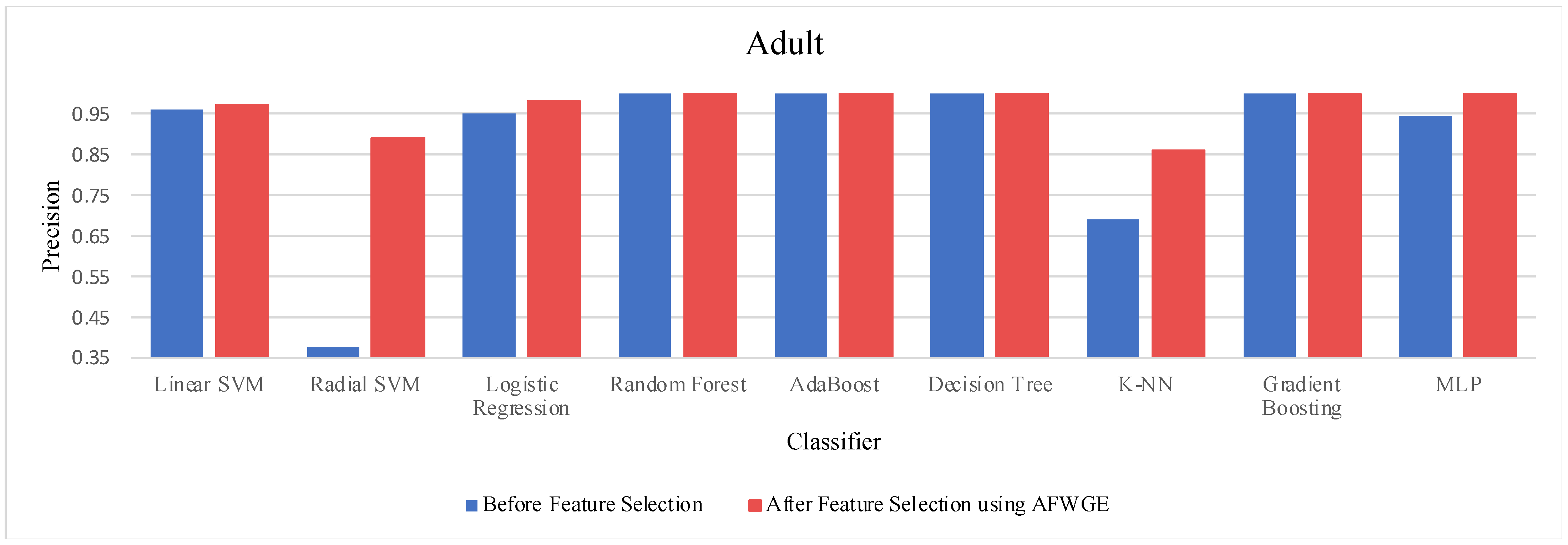
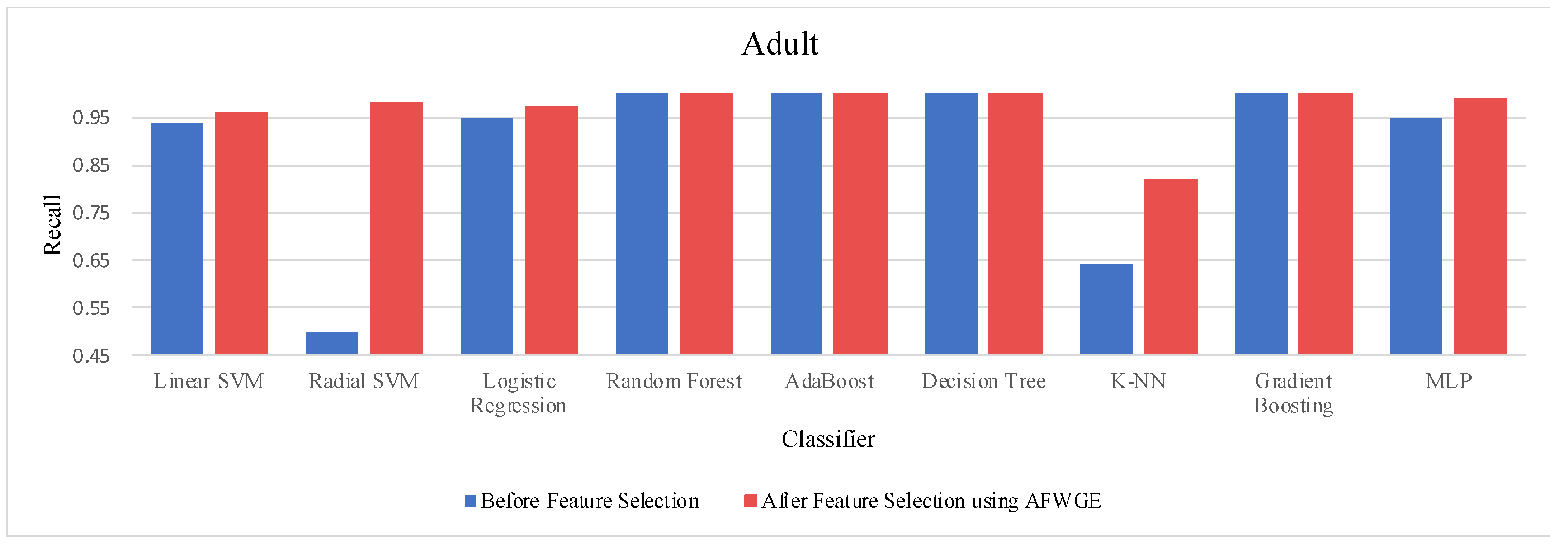
When comparing the performance using all features against the performance using only the important group of features across the three methods—Original Data, CERTIFAI, and AFWGE—on the Adult dataset, we obtained distinct outcomes, as shown in Table 3. For Original Data, there was no change in the accuracy of any of the nine classifiers. In contrast, the AFWGE method achieved enhanced accuracies for the L-SVM, R-SVM, LR, K-NN, and MLP classifiers, while the accuracies for RF, AdaBoost, DT, and Gradient Boosting remained unchanged. Meanwhile, the CERTIFAI method did not affect the accuracies of most classifiers; however, it led to an improvement in the K-NN classifier’s accuracy and a reduction in the MLP classifier’s accuracy.

Table 3. The percentage of average accuracy change when using each method on the Adult dataset for each classifier, where a positive change is in purple, a negative change is in orange, and the best for each classifier is indicated in bold.

Classifier	Original Data	AFWGE	CERTIFAI
L-SVM	0.0%	2.41%	0.0%
R-SVM	0.0%	9.21%	0.0%
LR	0.0%	3.15%	0.0%
RF	0.0%	0.0%	0.0%
AdaBoost	0.0%	0.0%	0.0%
DT	0.0%	0.0%	0.0%
K-NN	0.0%	14.38%	0.32%
Gradient Boosting	0.0%	0.0%	0.0%
MLP	0.0%	4.38%	−3.32%

The percentage change in accuracy across Original Data, AFWGE, and CERTIFAI reflects how each of the resulting groups of features affects the model’s ability to classify instances correctly. When comparing the values in Table 3, we can identify which method performs best and which performs worst. A positive percentage change in accuracy (highlighted in purple) indicates improvement, while a negative percentage change (highlighted in orange) indicates a reduction. The method with the highest percentage change (in bold) had the most significant positive impact on accuracy. In Table 2, the group of features selected by AFWGE shows the highest positive changes across multiple classifiers.

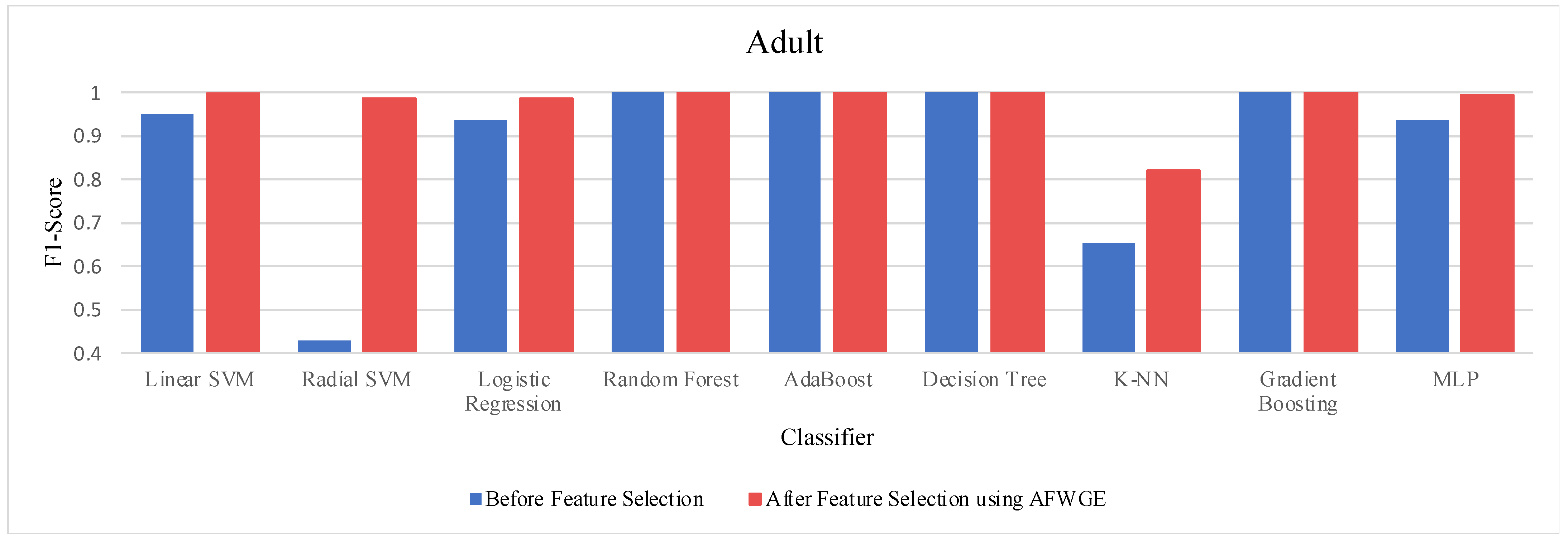
The threshold values for the PCCs were 0.6 and 0.7 for selecting the crucial group of features. The performance in terms of accuracy was the best for the most affected classifiers with the selected features at these thresholds, as shown in Figure 15. This increase in accuracy suggests that the features chosen at these PCC thresholds capture the main characteristics of the data, leading to the enhanced predictive performance of the classifiers.

Figure 15. Classifier accuracies on the Adult dataset for three rival methods using different PCC threshold values. (a) Linear SVM. (b) LR. (c) K-NN. (d) MLP.

Moreover, we conducted a Wilcoxon signed rank test to see if there was a statistically significant difference between the classifiers’ accuracies before and after using the group of features selected by AFWGE. The Wilcoxon test uses the following null (h₀) and alternative (h_A) hypotheses: h₀: the average value of accuracies is equal between the two groups; h_A: the average value of accuracies is not equal between the two groups. The test indicates that there was, indeed, a significant difference (at a significance level of α = 0.05); thus, the null hypothesis was rejected. This is verification that the average value of accuracies after using the selected feature group of AFWGE is significantly better than using all the Adult dataset features (Figure 16).

Figure 16. Classifier accuracies on the Adult dataset before and after using the group of features selected by AFWGE.

• Breast Cancer dataset:

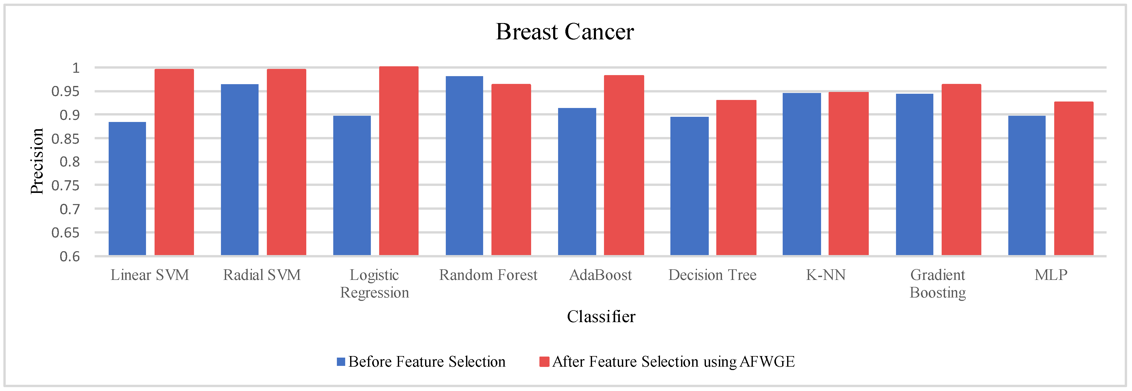
Table 4 shows the performance results of the three methods —Original Data, CERTIFAI, and AFWGE—on the Breast Cancer dataset. The results in Table 3 reveal the following findings: For Original Data, all nine classifiers, except L-SVM and LR, dropped in accuracy. In contrast, using AFWGE resulted in better accuracies for the L-SVM, R-SVM, LR, AdaBoost, DT, and Gradient Boosting classifiers while that for the K-NN classifier remained the same. However, there was a resultant decrease in accuracy for the RF and MLP classifiers. In contrast, when using the CERTIFAI method, the L-SVM, LR, DT, and Gradient Boosting classifiers showed enhanced accuracy, while there was a decrease in the accuracy of the R-SVM, RF, AdaBoost, K-NN, and MLP classifiers.

Table 4. The percentage of average accuracy change using each method on the Breast Cancer dataset for each classifier, where a positive change is in purple, a negative change is in orange, and the best for each classifier is in bold.

Classifier	Original Data	AFWGE	CERTIFAI
L-SVM	1.48%	4.44%	0.8%
R-SVM	−1.19%	0.71%	−0.18%
LR	0.99%	4.44%	1.17%
RF	−1.2%	−0.72%	−0.06%
AdaBoost	−1.7%	2.92%	−0.3%
DT	−1.37%	1.49%	0.43%
K-NN	−2.88%	0.0%	−1.02%
Gradient Boosting	−0.12%	1.46%	0.3%
MLP	−6.67%	−0.74%	−1.91%

Again, from Table 4, the percentage changes in accuracy for the Original Data, AFWGE, and CERTIFAI methods reveal how each method’s resulting group of features impacts the model’s ability to classify instances correctly. From this table, it is obvious that the group of features of AFWGE shows the highest positive changes across multiple classifiers.

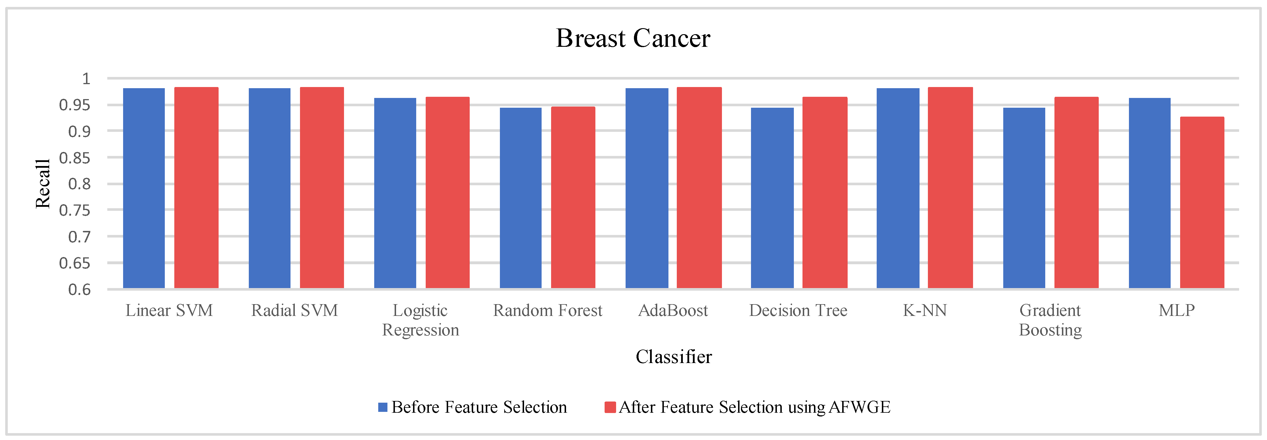
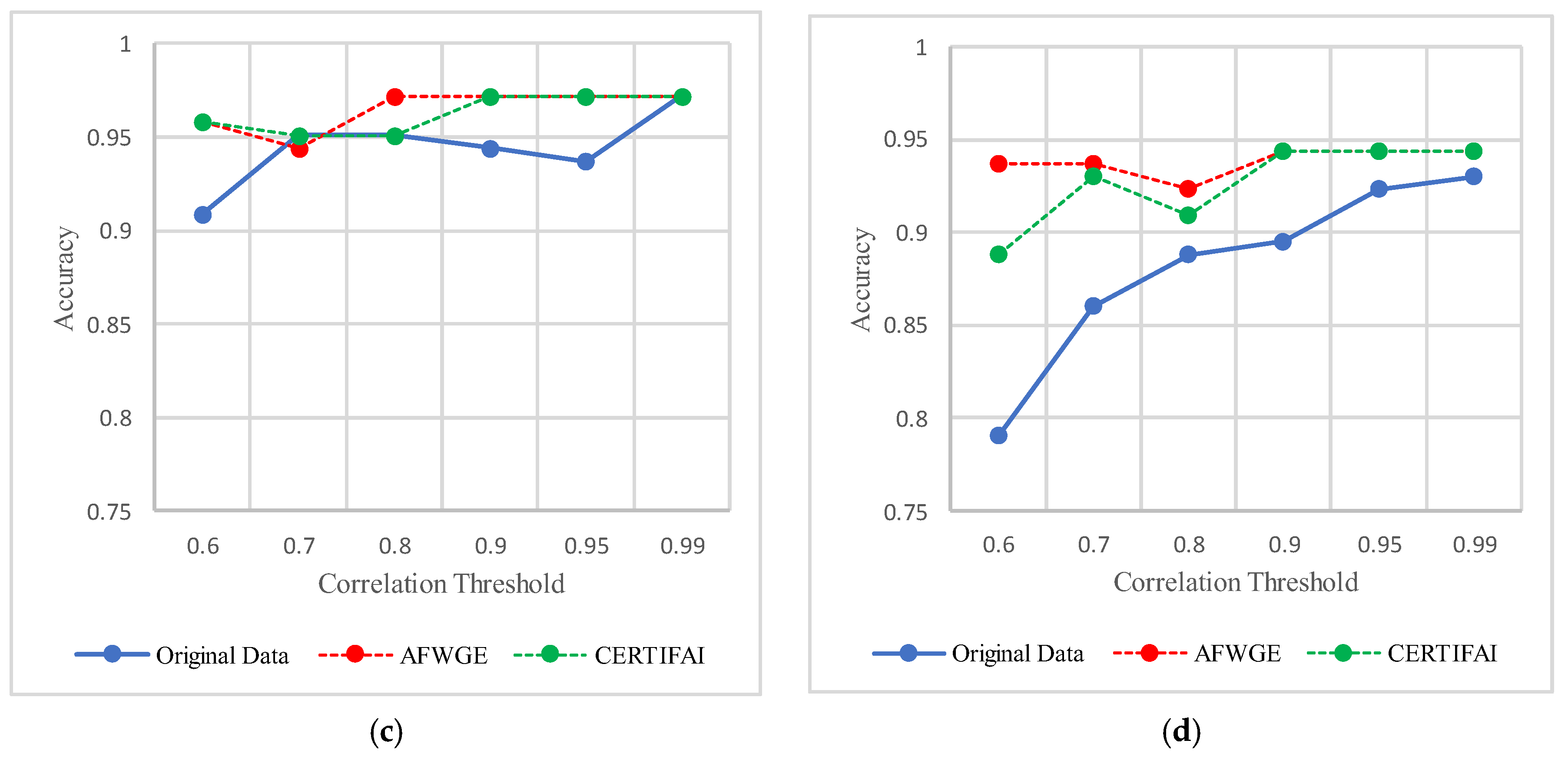
For the Breast Cancer dataset, the most important group of features was selected when the PCC threshold was equal to 0.6, 0.7, and 0.8. The selected features at these thresholds provided the best performance in terms of accuracy for the most affected classifiers, as shown in Figure 17. The selected features at these PCC thresholds capture the important characteristics of the data, enhancing the accuracy performance of the classifiers.

Figure 17. Classifier accuracies on the Breast Cancer dataset using three rival methods with different PCC threshold values. (a) Linear SVM. (b) LR. (c) K-NN. (d) MLP.

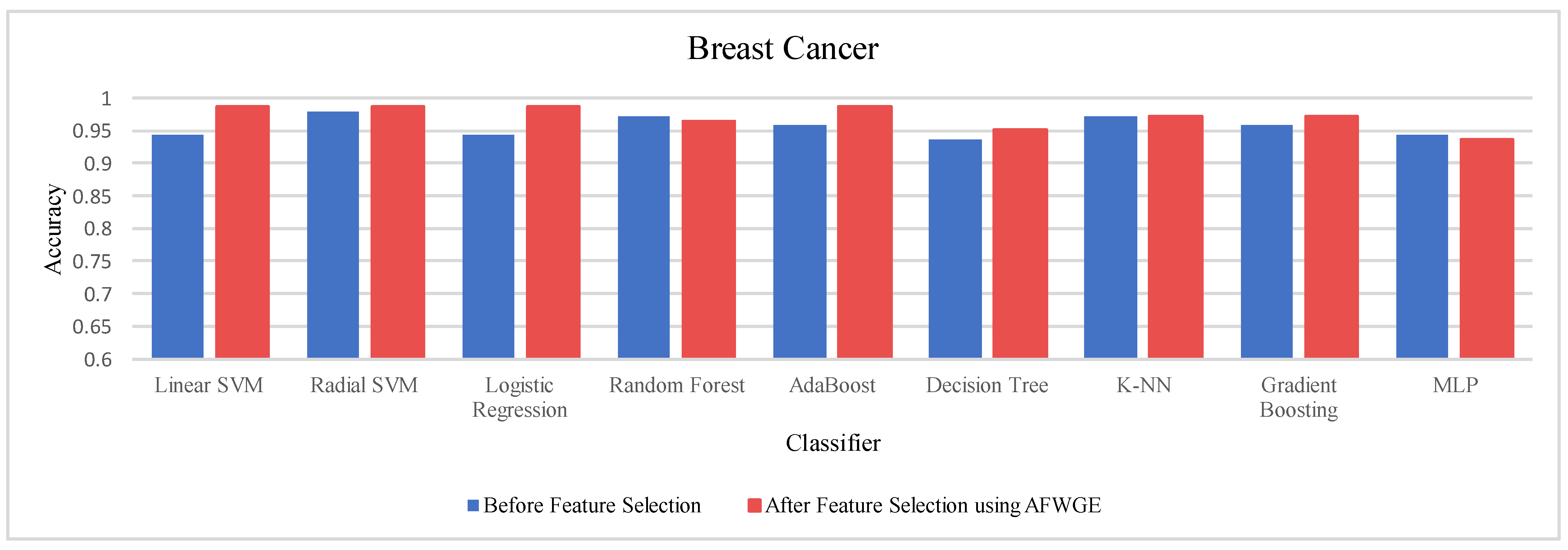
Again, the results were subjected to a Wilcoxon signed rank test to test the statistically significant difference between the classifier’s accuracies before and after using AFWGE’s selected group of features. Additionally, the test indicated that there was a significant difference at a significance level of α = 0.05; thus, the null hypothesis was rejected. This is verification that the average value of accuracy after using AFWGE’s selected crucial features is significantly better than that using all the Breast Cancer dataset features (Figure 18).

Figure 18. Classifier accuracies on the Breast Cancer dataset before and after using the group of features selected by AFWGE.

• Pima Indians Diabetes dataset:

Table 5 demonstrates the accuracy results on the Pima Indians Diabetes dataset for the three compared methods. When evaluating the results in Table 4, we observed distinct patterns, whereas, for Original Data, there was no change in the accuracy for any of the nine classifiers. In contrast, AFWGE improved the accuracies of the L-SVM, LR, RF, and MLP classifiers, though it had no effect on the R-SVM, AdaBoost, or DT classifiers. However, the accuracies of the K-NN and Gradient Boosting classifiers went down. For the CERTIFAI approach, the accuracy for the LR, AdaBoost, and K-NN classifiers increased, and the accuracy of the L-SVM, R-SVM, RF, DT, Gradient Boosting, and MLP classifiers decreased.

Table 5. The percentage of average accuracy change using each method for the Pima Indians Diabetes dataset for each classifier, where a positive change is in purple, a negative change is in orange, and the best for each classifier is in bold.

Classifier	Original Data	AFWGE	CERTIFAI
L-SVM	0.0%	1.4%	−0.35%
R-SVM	0.0%	0.0%	−0.46%
LR	0.0%	2.14%	0.24%
RF	0.0%	0.7%	−0.82%
AdaBoost	0.0%	0.0%	0.12%
DT	0.0%	0.0%	−0.38%
K-NN	0.0%	−0.77%	0.38%
Gradient Boosting	0.0%	−2.8%	−0.82%
MLP	0.0%	11.2%	−0.53%

Again, from Table 5, the most important group of features of AFWGE shows the highest positive changes across multiple classifiers for the Pima Indians Diabetes dataset, indicating the best performance among the three rival methods.

As shown in Figure 19, the selected features at a PCC threshold of 0.6 provided the best performance in terms of accuracy for the most affected classifiers.

Figure 19. Classifier accuracies on the Pima Indians Diabetes dataset using three rival methods with different PCC threshold values. (a) Linear SVM. (b) LR. (c) K-NN. (d) MLP.

Once more, we performed a Wilcoxon signed rank test between the classifiers’ accuracies before and after using the most important group of features of AFWGE. The results, again, showed that there was a significant difference at α = 0.05; thus, the null hypothesis was rejected. Thus, we can conclude that the average value of accuracy after AFWGE is significantly better than using all the Pima Indians Diabetes dataset’s features (Figure 20).

Figure 20. Classifier accuracies on the Pima Indians Diabetes dataset before and after using the group of features selected by AFWGE.

• Iris dataset:

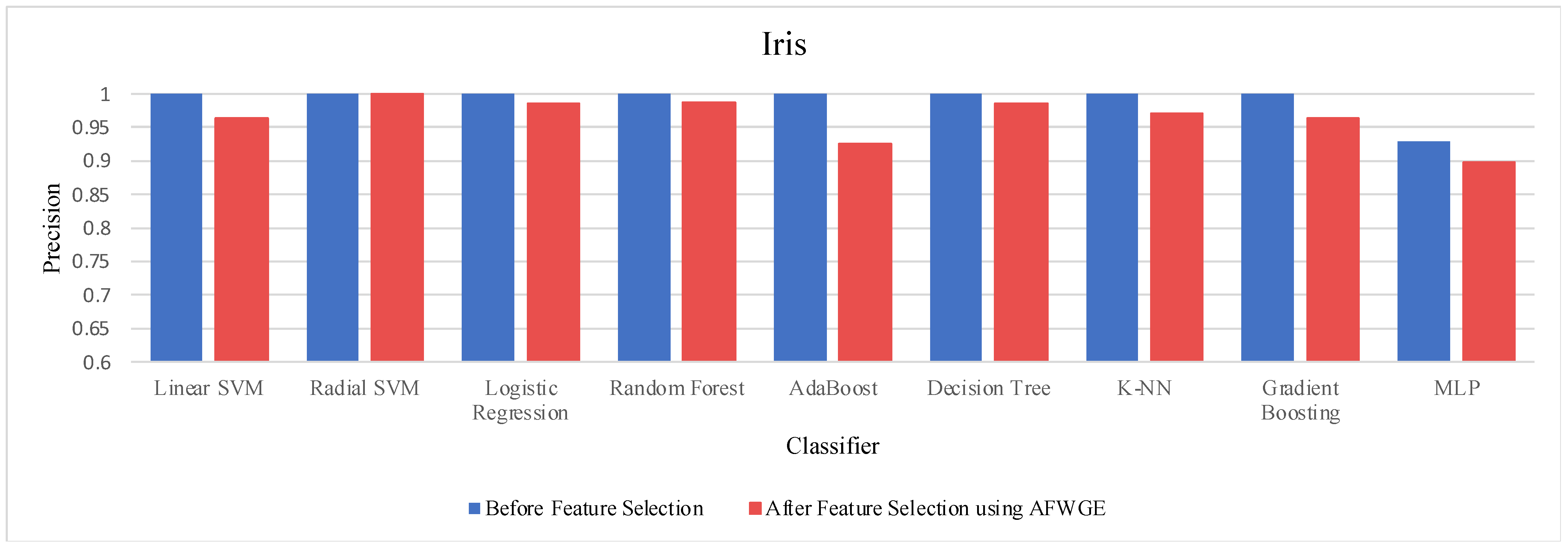
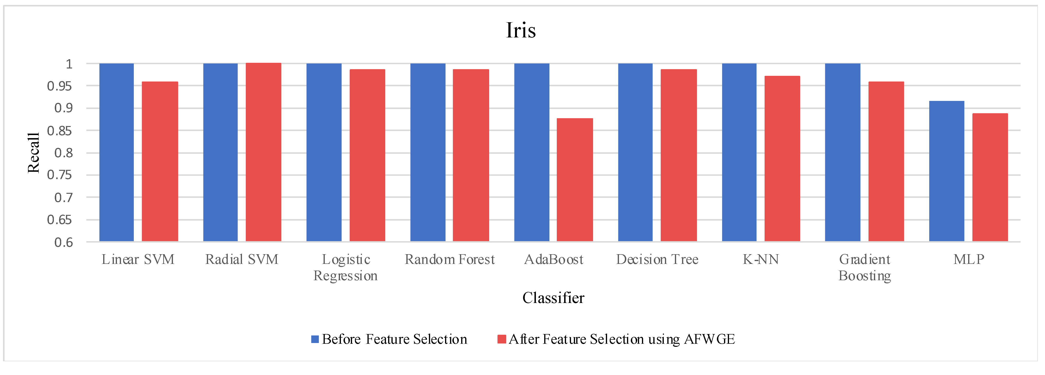
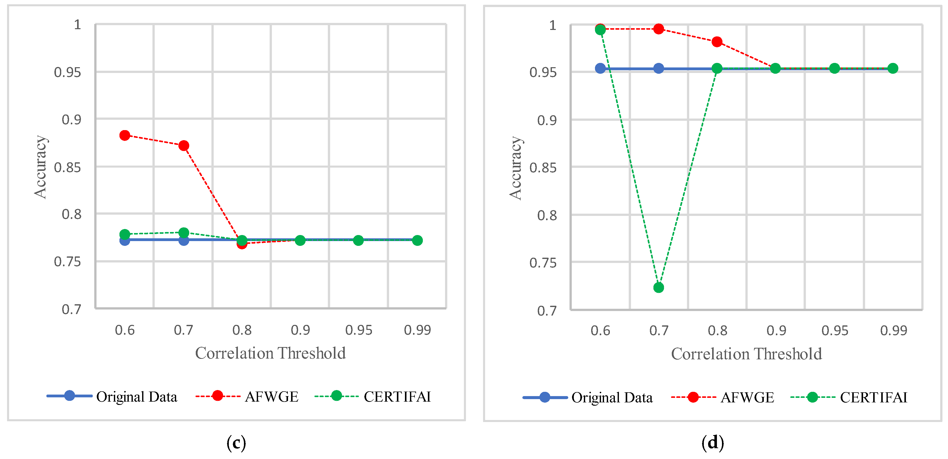
Prior to utilizing the selected group of features, all classifiers employed on the Iris dataset demonstrated exceptionally high accuracies, nearly equivalent to 1.0, often indicating overfitting. Certain characteristics of the Iris dataset, such as its small size, low dimensionality, and distinct class separability, can contribute to overfitting. However, when the Original Data method was used, the accuracies of all nine classifiers were reduced, as shown in Table 6. Similarly, the AFWGE method resulted in a moderate decrease in accuracies for all nine classifiers, with the exception of the R-SVM classifier, which maintained the same accuracy. The CERTIFAI method also led to reduced accuracies for all nine classifiers. Nevertheless, the results in Table 6 demonstrate that the most important group of features of AFWGE exhibited the minimum reduction in accuracy across multiple classifiers.

Table 6. The percentage of average accuracy change using each method for the Iris dataset for each classifier, where a negative change is in orange, and the best for each classifier is in bold.

Classifier	Original Data	AFWGE	CERTIFAI
L-SVM	−9.21%	−3.95%	−5.26%
R-SVM	−7.89%	0.0%	−2.63%
LR	−8.33%	−1.32%	−3.51%
RF	−10.96%	−1.32%	−4.39%
AdaBoost	−18.42%	−11.84%	−12.72%
DT	−17.54%	−1.32%	−6.58%
K-NN	−8.77%	−2.63%	−4.39%
Gradient Boosting	−11.84%	−3.95%	−6.14%
MLP	−9.52%	−2.86%	−4.76%

As shown in Figure 21, the most important group of features was selected when the PCC threshold was equal to 0.9, 0.95, and 0.99. This limited the reduction in accuracy at these PCC thresholds; however, it effectively minimized overfitting, demonstrating that the selected features retained the essential characteristics of the data without allowing the classifiers to overfit. Therefore, the selected features are the most important features, supporting both generalizability and interpretability.

Figure 21. Classifier accuracies on the Iris dataset using the three rival methods with different PCC threshold values. (a) Linear SVM. (b) LR. (c) K-NN. (d) MLP.

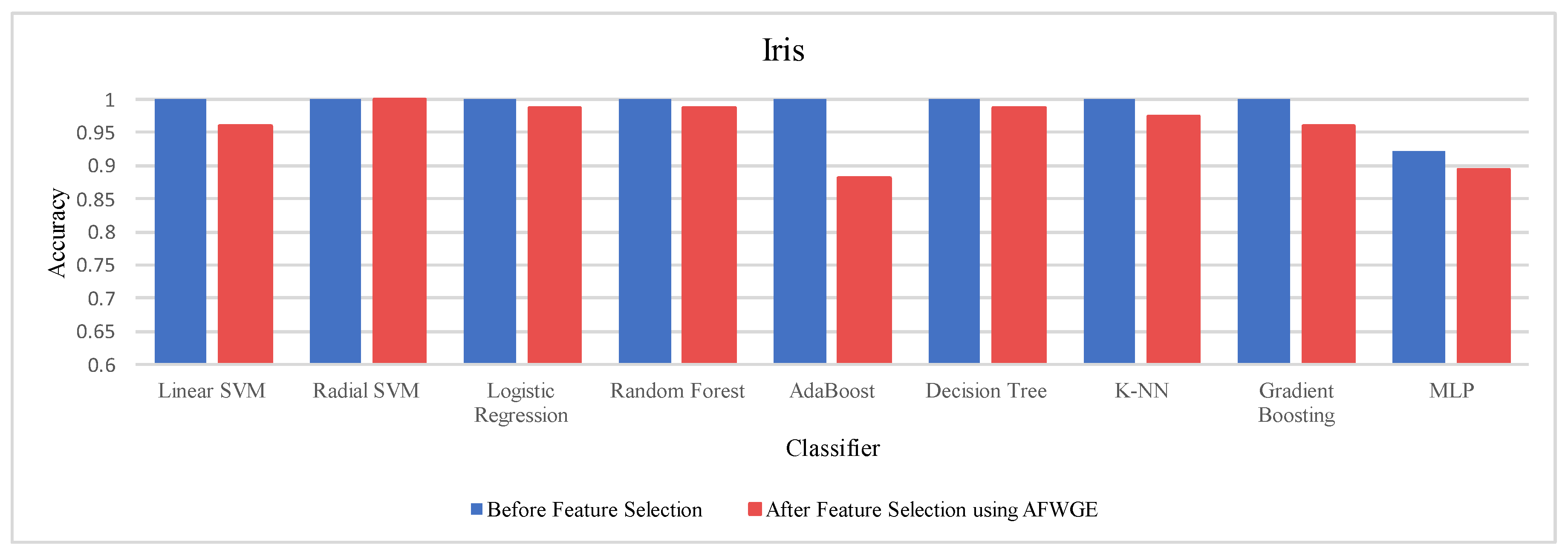
We ran another Wilcoxon signed rank test to check whether there was a statistically significant difference between the classifiers’ accuracies before and after using the most important group of features of AFWGE. Once again, the findings demonstrated a significant difference at a significance level of α = 0.05; thus, the null hypothesis was rejected. Therefore, it can be concluded that the average value of the accuracies after using AFWGE is significantly better than using all the Iris dataset features since it reduces overfitting (Figure 22).

Figure 22. Classifier accuracies on the Iris dataset before and after using the group of features selected by AFWGE.

5.2.3. Precision

The results demonstrate a clear improvement in classifiers’ performance when using the selected group of features, particularly with the AFWGE method. This highlights the effectiveness of AFWGE in enhancing feature selection. The details and comprehensive analysis of these results are provided in the Appendix (See Appendix A).

5.2.4. Recall

Using the selected set of features, especially the AFWGE method, significantly improves classifier performance, according to the results. This demonstrates how effectively AFWGE improves feature selection. Results are thoroughly analyzed and detailed in the Appendix (See Appendix B).

5.2.5. F1-Score

The results show that classifier performance is much enhanced by using the selected group of features, specially the AFWGE method. This illustrates that AFWGE enhances feature selection effectively. The results are presented in the appendix with analysis (See Appendix C).

5.3. Results: Analysis and Discussion

The detailed results presented above show how the classifiers’ performance improved using the resulting selected group of features, especially when using the AFWGE method. The important group of features obtained through the weights of AFWGE with the PCC improved all performance metrics for all the tested classifiers. Since AFWGE provided the highest positive percentage change for all the classifiers’ performance metrics, we used the Wilcoxon test to evaluate the significance of AFWGE’s superiority over the Original Data and CERTIFAI methods. The results of this testing are presented in Table 7, where the method(s) with statistically significant performance is (are) indicated in each case.

Table 7. Superior method(s) based on the Wilcoxon test for each performance criterion for all nine classifiers.

Dataset	Performance Criteria
	Accuracy	Precision	Recall	F1 Score
Adult	AFWGE	AFWGE	AFWGE	AFWGE
Breast Cancer	AFWGE	AFWGE	AFWGE/CERTIFAI	AFWGE
Pima Indians Diabetes	AFWGE	* AFWGE/CERTIFAI	AFWGE/Original Data	AFWGE
Iris	AFWGE	AFWGE	AFWGE	AFWGE

* AFWGE performed better than Original Data but not as well as CERTIFAI. However, CERTIFAI outperformed neither Original Data nor AFWGE.

Moreover, a summary of the statistical significance results using the Wilcoxon test to indicate whether performance was significantly enhanced when using the group of features selected by AFWGE is shown in Table 8. From this table, it is demonstrated that AFWGE provided a significant improvement across all four performance metrics for all nine classifiers on the four datasets, except for precision and recall on the Pima Indians Diabetes dataset. Nonetheless, on this dataset, the Wilcoxon test indicated that AFWGE provided a significant improvement in the F1 score, which is defined as the harmonic mean of precision and recall and is derived from the confusion matrix; thus, it can completely describe the outcome of a classification task [45].

Table 8. Summary of the Wilcoxon test for all performance criteria used to assess the enhancement in performance before and after using the selected group of features for the AFWGE method and each dataset. Yes denotes a significant enhancement, and No denotes no significant enhancement.

Dataset	Performance Criteria
	Accuracy	Precision	Recall	F1 Score
Adult	Yes	Yes	Yes	Yes
Breast Cancer	Yes	Yes	Yes	Yes
Pima Indians Diabetes	Yes	No	No	Yes
Iris	Yes	Yes	Yes	Yes

In fact, out of the four datasets, only the Pima Indians Diabetes dataset has an imbalance toward the negative class (nondiabetic), since 65% of the instances are classified as not having diabetes, and 35% are classified as having diabetes. An ML model’s ability to accurately detect instances of the minority class (diabetic) can be negatively affected by this imbalance if the model becomes biased toward the majority class (nondiabetic). The overall accuracy and F1 score may have improved for this reason; these measures can conceal weak performance when applied to minority classes. Because the majority class is bigger and controls the measure, accuracy might become better. Since the F1 score is the average of precision and recall, it can show growth even if one of the parts is much lower, in case the other part becomes good enough. It is more important to correctly identify the minority class when using precision and recall measures. Therefore, if the model performance worsens when correctly predicting the positive class (diabetic), it has a stronger effect on precision and recall [46].

Finally, it is worth noting that lower metric results do not necessarily mean worse performance. For example, on the Iris dataset, most performance criteria were approximately equal to one (i.e., 100%) before using the selected group of features, which indicated overfitting. In fact, FS is a widely recognized task in ML, which has the aim of reducing the chances of overfitting a model on a dataset [47]. Therefore, the performance criteria with the Iris dataset were reduced significantly using the selected group of features.

5.4. Analysis of the Importance of a Group of Features vs. Individual Feature Importance

The strategy for identifying the contribution of each feature through feature importance vs. the contribution of a group of features was also significant in the current analysis. Table 9 shows the selected group of features for each dataset obtained via the AFWGE method with the PCC, as explained previously. Mostly, correlation analysis is performed to identify hidden patterns in data (e.g., as in [37]) to distinguish the most important group of features, i.e., the group of features that collectively have a crucial impact on performance. For example, as can be seen for the Pima Indians Diabetes dataset, the feature importance ranking using AFWGE [13], LIME (local interpretable model-agnostic), and LPI (local permutation importance) explanations [48] of “Blood Pressure” is higher than for “Insulin”. However, the most important group of features of AFWGE inferred from our FS results, as shown in Table 9, does not reveal the same information. From this table, we can see that the best performance of the classifiers on the Pima Indians Diabetes dataset included “Insulin” instead of “Blood Pressure”, although the latter had higher importance than “Insulin” as an individual feature (as mentioned above).

Table 9. The most important group of features selected by AFWGE on each dataset.

Dataset	The Group of Features Selected by AFWGE
Adult	Eight features: [age, education, education_num, occupation, race, sex, capital_gain, hours_per_week]
Breast Cancer	Thirteen features: [Mean_Radius, Mean_Texture, Mean_Perimeter, Mean_Area, Mean_Smoothness, Mean_Compactness, Mean_Concave_Points, Mean_Symmetry, SE_Radius, SE_Area, Worst_Area, Worst_Concavity, Worst_Fractal_Dimension]
Pima Indians Diabetes	Six features: [Pregnancies, Glucose, Insulin, BMI, DiabetesPedigreeFunction, Age]
Iris	Three features: [SepalLengthCm, SepalWidthCm, PetalLengthCm]

Thus, we inferred that the process of determining which group of features in a learning model’s dataset is the most important for performance, and this is distinct from the process of simply calculating the importance of each individual feature and selecting the highest among them. The concept of feature importance focuses on the contribution of individual features to the predictions made by the model. On the other hand, determining which features constitute an important group requires an understanding of how different combinations of features interact with one another and collectively influence the model’s performance. As previously mentioned, an example is the case of the Pima Indians Diabetes dataset, where “Insulin” was included in the most important group of features instead of “Blood Pressure”, even though it had lower weight as an individual feature of importance. It seems that, somehow, “Insulin”, together with other selected important features, influenced the decision of the model and compensated for the presence of “Blood Pressure” in the selected feature set. When using the PCC, we could identify the feature groups that best captured the most important patterns to gain a deeper understanding of the data’s fundamental structure. For instance, in high-stakes domains such as healthcare or finance, users can rely on AFWGE-derived feature weights to focus on the most relevant relationships among the features, making counterfactual explanations more actionable and aligned with domain-specific requirements.

The utilization of the counterfactual explanations of AFWGE, with its embedded feature weights, contribute to the effectiveness of the PCC approach. Thus, it is possible to identify the most important group of features more effectively by combining these weights with correlation analysis. AFWGE provides interpretability by adaptively learning feature weights throughout the optimization process. This continuous adaptation allows AFWGE to capture the dynamic influence of each feature within the counterfactual generation process. Furthermore, the incorporation of the PCC allows the method to reduce feature redundancy, providing more stable and relevant insights for end users to understand feature relationships and dependencies. Thus, our proposed method helps end users focus on the most critical features to recognize which features most significantly influence the model’s predictions rather than being confused by redundant or less informative ones.

This helps to ensure that the selected groups of features are both individually relevant and collectively significant in improving the learning model’s performance.

6. Conclusions

Feature selection (FS) is an important process in machine learning (ML), where the goal is to find and select the most relevant features from a dataset to enhance the model’s performance and reduce overfitting. Our proposed method leverages the feature weights obtained using the adaptive feature weight genetic explanation (AFWGE) method, combined with the Pearson correlation coefficient (PCC), to identify the most important group of features, thereby optimizing FS and enhancing model performance. Extensive testing was performed using the proposed approach on four real-world datasets that encompass both continuous and categorical features, each with nine separate classifiers. By adopting a comprehensive approach, we were able to evaluate the effectiveness of the proposed method with different models and with various types of data.

The results demonstrated that the important group of features identified by AFWGE, together with the PCC, offers a significant improvement in terms of accuracy, precision (Appendix A), recall (Appendix B), and F1 score on most datasets and for most classifier models. Moreover, the results demonstrated the superiority of weights from AFWGE over the number of feature changes from CERTIFAI and the Original Data values with the PCC in enhancing the model’s performance.

This study aimed to improve the interpretability of AI models through crucial features’ selection. Machine learning interpretability is becoming increasingly important, especially as ML algorithms grow more complex. In many cases, less performant but explainable models are preferred over more performant black box models, highlighting the need for transparency in decision making. This is why research around XAI has recently become a growing field achieving significant advances. Would users, model developers, and regulators feel confident using a machine learning model if they cannot explain what it does? XAI techniques in FS, such as AFWGE, aim to address this by explaining why certain features are selected or considered important by the model, helping to clarify the relationship between input features and the model’s decision-making process. This is where our AFWGE feature weights with the PCC can be highly beneficial; they provide interpretability by indicating the influence of each feature on the target, making it applicable to any ML model. Focusing on the most important group of features for reversing the decision and producing the desired outcome will help not only individuals, model developers, and regulators to enhance the model’s behavior but also with understanding its behavior and making more informed decisions. This effort will help bridge the gap between model accuracy and explainability, leading to more trustworthy AI systems.

Future work will involve extending the proposed method assessment against various existing XAI methods, with additional testing on higher-dimensional and noisier datasets to ensure the method’s robust applicability and performance across diverse scenarios. Moreover, primarily due to the adaptive nature of feature weights and the repeated evaluations required for optimization, this resulted in increased processing times for the AFWGE method. Thus, one of the future goals is optimizing computational efficiency, possibly through leveraging external libraries to parallelize the process. Additionally, we plan to improve the accuracy of the techniques and investigate the performance of hybrid approaches to identify the crucial group of features by integrating AFWGE with other XAI techniques, such as LIME or SHAP.

References

1. Gunning, D.; Vorm, E.; Wang, J.Y.; Turek, M. DARPA’s Explainable AI (XAI) Program: A Retrospective. Appl. AI Lett. 2021, 2, e61. [Google Scholar] [CrossRef]
2. Doshi-Velez, F.; Kim, B. Towards A Rigorous Science of Interpretable Machine Learning. arXiv 2017, arXiv:1702.08608. [Google Scholar]
3. Miller, T. Explanation in Artificial Intelligence: Insights from the Social Sciences. arXiv 2018, arXiv:1706.07269. [Google Scholar] [CrossRef]
4. Mittelstadt, B.; Russell, C.; Wachter, S. Explaining Explanations in AI. In Proceedings of the Conference on Fairness, Accountability, and Transparency, Atlanta, GA, USA; 2019; pp. 279–288. [Google Scholar] [CrossRef]
5. Celar, L.; Byrne, R.M.J. How People Reason with Counterfactual and Causal Explanations for Artificial Intelligence Decisions in Familiar and Unfamiliar Domains. Mem. Cognit. 2023, 51, 1481–1496. [Google Scholar] [CrossRef]
6. Rasool, A.; Shahzad, M.I.; Aslam, H.; Chan, V. Emotion-Aware Response Generation Using Affect-Enriched Embeddings with LLMs. arXiv 2024, arXiv:2410.01306. [Google Scholar]
7. Abid, A.; Yuksekgonul, M.; Zou, J. Meaningfully Debugging Model Mistakes Using Conceptual Counterfactual Explanations. In Proceedings of the 39th International Conference on Machine Learning, PMLR, Baltimore, MD, USA, 17–23 July 2022; Chaudhuri, K., Jegelka, S., Song, L., Szepesvari, C., Niu, G., Sabato, S., Eds.; Volume 162, pp. 66–88. [Google Scholar]
8. Akula, A.R.; Wang, K.; Liu, C.; Saba-Sadiya, S.; Lu, H.; Todorovic, S.; Chai, J.; Zhu, S.-C. CX-ToM: Counterfactual Explanations with Theory-of-Mind for Enhancing Human Trust in Image Recognition Models. iScience 2022, 25, 103581. [Google Scholar] [CrossRef]
9. Warren, G.; Byrne, R.M.J.; Keane, M.T. Categorical and Continuous Features in Counterfactual Explanations of AI Systems. In Proceedings of the 28th International Conference on Intelligent User Interfaces, ACM, Sydney, NSW, Australia, 27 March 2023; pp. 171–187. [Google Scholar]
10. Turati, G.; Dacrema, M.F.; Cremonesi, P. Feature Selection for Classification with QAOA. In Proceedings of the 2022 IEEE International Conference on Quantum Computing and Engineering (QCE), Broomfield, CO, USA, 18–23 September 2022; pp. 782–785. [Google Scholar]
11. Parr, T.; Wilson, J.D.; Hamrick, J. Nonparametric Feature Impact and Importance. Inf. Sci. 2020, 653, 119563. [Google Scholar] [CrossRef]
12. Kumar, S.; Bhushan, B.; Bhambhu, L.; Thakur, M.; Mohapatra, U.M.; Choubey, D.K. Medical Datasets Classification Using a Hybrid Genetic Algorithm for Feature Selection Based on Pearson Correlation Coefficient. In Proceedings of the 2022 International Conference on Machine Learning, Computer Systems and Security (MLCSS), Bhubaneswar, India, 5–6 August 2022; pp. 214–218. [Google Scholar]
13. AlJalaud, E.; Hosny, M. Counterfactual Explanation of AI Models Using an Adaptive Genetic Algorithm With Embedded Feature Weights. IEEE Access 2024, 12, 74993–75009. [Google Scholar] [CrossRef]
14. Sharma, S.; Henderson, J.; Ghosh, J. CERTIFAI: A Common Framework to Provide Explanations and Analyse the Fairness and Robustness of Black-Box Models. In Proceedings of the AAAI/ACM Conference on AI, Ethics, and Society, New York, NY, USA, 7–9 February 2020; pp. 166–172. [Google Scholar]
15. Wachter, S.; Mittelstadt, B.; Russell, C. Counterfactual Explanations Without Opening the Black Box: Automated Decisions and the GDPR. SSRN Electron. J. 2017, 31, 841. [Google Scholar] [CrossRef]
16. Ustun, B.; Spangher, A.; Liu, Y. Actionable Recourse in Linear Classification. In Proceedings of the Conference on Fairness, Accountability, and Transparency, Atlanta, GA, USA, 29–31 January 2019; pp. 10–19. [Google Scholar] [CrossRef]
17. Yeh, I.-C.; Lien, C. The Comparisons of Data Mining Techniques for the Predictive Accuracy of Probability of Default of Credit Card Clients. Expert Syst. Appl. 2009, 36, 2473–2480. [Google Scholar] [CrossRef]
18. Schleich, M.; Geng, Z.; Zhang, Y.; Suciu, D. GeCo: Quality Counterfactual Explanations in Real Time. arXiv 2021, arXiv:2101.01292. [Google Scholar] [CrossRef]
19. Karimi, A.-H.; Barthe, G.; Balle, B.; Valera, I. Model-Agnostic Counterfactual Explanations for Consequential Decisions. In Proceedings of the 23rd International Conference on Artificial Intelligence and Statistics (AISTATS) 2020, Palermo, Italy, 26–28 August 2020; Volume 108, pp. 12–27. [Google Scholar]
20. Mahajan, D.; Tan, C.; Sharma, A. Preserving Causal Constraints in Counterfactual Explanations for Machine Learning Classifiers; Proc CausalML Workshop NeurIPS. arXiv 2019, arXiv:1912.03277. [Google Scholar]
21. Wexler, J.; Pushkarna, M.; Bolukbasi, T.; Wattenberg, M.; Viegas, F.; Wilson, J. The What-If Tool: Interactive Probing of Machine Learning Models. IEEE Trans. Vis. Comput. Graph. 2019, 26, 56–65. [Google Scholar] [CrossRef]
22. Guo, C.; Gardner, J.R.; You, Y.; Wilson, A.G.; Weinberger, K.Q. Simple Black-Box Adversarial Attacks. In Proceedings of the 36th International Conference on Machine Learning, Long Beach, CA, USA, 9–15 June 2019. [Google Scholar]
23. Dastile, X.; Celik, T.; Vandierendonck, H. Model-Agnostic Counterfactual Explanations in Credit Scoring. IEEE Access 2022, 10, 69543–69554. [Google Scholar] [CrossRef]
24. Becker, B.; Kohavi, R. Adult. UCI Mach. Learn. Repos. 1996, 10, C5XW20. [Google Scholar]
25. Wolberg, W.; Mangasarian, O.; Street, N.; Street, W. Breast Cancer Wisconsin (Diagnostic). UCI Mach. Learn. Repos. 1995, 10, C5DW2B. [Google Scholar]
26. Pima Indians Diabetes Database. 1988. Available online: https://www.kaggle.com/datasets/uciml/pima-indians-diabetes-database (accessed on 4 June 2024).
27. Fisher, R.A. Iris. 1988. Available online: https://archive.ics.uci.edu/dataset/53/iris (accessed on 4 June 2024).
28. Ketu, S.; Mishra, P.K. Scalable Kernel-Based SVM Classification Algorithm on Imbalance Air Quality Data for Proficient Healthcare. Complex Intell. Syst. 2021, 7, 2597–2615. [Google Scholar] [CrossRef]
29. Sharma, A.; Mishra, P.K. Performance Analysis of Machine Learning Based Optimized Feature Selection Approaches for Breast Cancer Diagnosis. Int. J. Inf. Technol. 2022, 14, 1949–1960. [Google Scholar] [CrossRef]
30. Mishra, S. Financial Management and Forecasting Using Business Intelligence and Big Data Analytic Tools. Int. J. Financ. Eng. 2018, 5, 1850011. [Google Scholar] [CrossRef]
31. Doreswamy; Hooshmand, M.K.; Gad, I. Feature Selection Approach Using Ensemble Learning for Network Anomaly Detection. CAAI Trans. Intell. Technol. 2020, 5, 283–293. [Google Scholar] [CrossRef]
32. Yaping, Z.; Changyin, Z. Gene Feature Selection Method Based on Relieff and Pearson Correlation. In Proceedings of the 2021 3rd International Conference on Applied Machine Learning, Changsha, China, 23–25 July 2021; IEEE: Piscataway, NJ, USA, 2021; pp. 15–19. [Google Scholar]
33. Kononenko, I.; Simec, E.; Robnik-Sikonja, M. Overcoming the Myopia of Inductive Learning Algorithms with RELIEFF. Appl. Intell. 1997, 7, 39–55. [Google Scholar] [CrossRef]
34. Ponniah, T. Machine Learning Model for Breast Cancer Data Analysis Using Triplet Feature Selection Algorithm. IETE J. Res. 2023, 69, 1789–1799. [Google Scholar]
35. Rasool, A.; Bunterngchit, C.; Tiejian, L.; Islam, M.d.R.; Qu, Q.; Jiang, Q. Improved Machine Learning-Based Predictive Models for Breast Cancer Diagnosis. Int. J. Environ. Res. Public. Health 2022, 19, 3211. [Google Scholar] [CrossRef]
36. Al-Shalabi, L. New Feature Selection Algorithm Based on Feature Stability and Correlation. IEEE Access 2022, 10, 4699–4713. [Google Scholar] [CrossRef]
37. Atmakuru, A.; Di Fatta, G.; Nicosia, G.; Badii, A. Improved Filter-Based Feature Selection Using Correlation and Clustering Techniques. In Proceedings of the Machine Learning, Optimization, and Data Science; Pontignano, Italy, 18–22 September 2022, Nicosia, G., Ojha, V., La Malfa, E., La Malfa, G., Pardalos, P.M., Umeton, R., Eds.; Springer Nature: Cham, Switzerland, 2024; pp. 379–389. [Google Scholar]
38. Sharma, M.; Kaur, P. A Comprehensive Analysis of Nature-Inspired Meta-Heuristic Techniques for Feature Selection Problem. Arch. Comput. Methods Eng. 2021, 28, 1103–1127. [Google Scholar] [CrossRef]
39. Blum, A.L.; Langley, P. Selection of Relevant Features and Examples in Machine Learning. Artif. Intell. 1997, 97, 245–271. [Google Scholar] [CrossRef]
40. Koller, D.; Sahami, M. Toward Optimal Feature Selection; Stanford InfoLab: Stanford, CA, USA, 1996. [Google Scholar]
41. Ooi, C.H.; Chetty, M.; Teng, S.W. Differential Prioritization in Feature Selection and Classifier Aggregation for Multiclass Microarray Datasets. Data Min. Knowl. Discov. 2007, 14, 329–366. [Google Scholar] [CrossRef]
42. Rasool, A.; Jiang, Q.; Qu, Q.; Kamyab, M.; Huang, M. HSMC: Hybrid Sentiment Method for Correlation to Analyze COVID-19 Tweets. In Advances in Natural Computation, Fuzzy Systems and Knowledge Discovery, Proceedings of the 15th International Conference on Natural Computation, Fuzzy Systems and Knowledge Discovery (ICNC-FSKD 2019), Kunming, China, 20–22 July 2019; Xie, Q., Zhao, L., Li, K., Yadav, A., Wang, L., Eds.; Springer International Publishing: Cham, Switzerland, 2022; pp. 991–999. [Google Scholar]
43. Liu, Y.; Mu, Y.; Chen, K.; Li, Y.; Guo, J. Daily Activity Feature Selection in Smart Homes Based on Pearson Correlation Coefficient. Neural Process. Lett. 2020, 51, 1771–1787. [Google Scholar] [CrossRef]
44. Fathi, H.; AlSalman, H.; Gumaei, A.; Manhrawy, I.I.M.; Hussien, A.G.; El-Kafrawy, P. An Efficient Cancer Classification Model Using Microarray and High-Dimensional Data. Comput. Intell. Neurosci. 2021, 2021, 7231126. [Google Scholar] [CrossRef]
45. Chicco, D.; Jurman, G. The Advantages of the Matthews Correlation Coefficient (MCC) over F1 Score and Accuracy in Binary Classification Evaluation. BMC Genom. 2020, 21, 6. [Google Scholar] [CrossRef]
46. He, H.; Ma, Y. Imbalanced Learning: Foundations, Algorithms, and Applications; Wiley: Hoboken, NJ, USA, 2013; ISBN 978-1-118-64633-5. [Google Scholar]
47. Ahmad, H.F.; Mukhtar, H.; Alaqail, H.; Seliaman, M.; Alhumam, A. Investigating Health-Related Features and Their Impact on the Prediction of Diabetes Using Machine Learning. Appl. Sci. 2021, 11, 1173. [Google Scholar] [CrossRef]
48. Rahnama, A.H.A.; Butepage, J.; Geurts, P.; Bostrom, H. Evaluating Local Explanations Using White-Box Models. arXiv 2022, arXiv:2106.02488. [Google Scholar]
Disclaimer/Publisher’s Note: The statements, opinions and data contained in all publications are solely those of the individual author(s) and contributor(s) and not of MDPI and/or the editor(s). MDPI and/or the editor(s) disclaim responsibility for any injury to people or property resulting from any ideas, methods, instructions or products referred to in the content.
Article Metrics
Citations
Article Access Statistics
Multiple requests from the same IP address are counted as one view.