
A New Methodology for the Development of Efficient Multistep Methods for First-Order Initial Value Problems with Oscillating Solutions V: The Case of the Open Newton–Cotes Differential Formulae


Abstract
1. Introduction
- Section 2 laid the groundwork for the theory that determines the phase lag and amplification factor of Open Newton–Cotes Differential Formulae (ONCDF). Since these approaches are part of a particular class of explicit multistep procedures, the theory given in [25] will be used as a basis for developing the general theory. The direct equations for the phase-lag and amplification-factor computations will be generated here.
- Section 3 presents the strategies to reduce or vanish the phase lag and the amplification factor and the derivatives of the phase lag and the amplification factor.
- Section 4 introduces the Open Newton–Cotes differential method that will be used to examine.
- Section 5 investigates the amplification-fitted Open Newton–Cotes differential method of sixth algebraic order with a phase lag of order six.
- Section 6 investigates the phase-fitted and amplification-fitted Open Newton–Cotes differential method of algebraic order Six.
- Section 7 investigates the phase-fitted and amplification-fitted Open Newton–Cotes differential method of algebraic order six with vanished the first derivative of the amplification factor.
- Section 8 investigates the phase-fitted and amplification-fitted Open Newton–Cotes differential method of algebraic order six with the eliminated first derivative of the phase lag.
- Section 9 investigates the phase-fitted and amplification-fitted Open Newton–Cotes differential method of algebraic order six with the eliminated first derivative of the phase lag and the first derivative of the amplification factor.
- Section 10 investigates the phase-fitted and amplification-fitted Open Newton–Cotes differential method of algebraic order five with the eliminated first and second derivatives of the amplification factor.
- Section 11 investigates the phase-fitted and amplification-fitted Open Newton–Cotes differential method of algebraic order four with the eliminated first and second derivatives of the phase lag.
- Section 12 investigates the Open Newton–Cotes differential methods as symplectic integrators.
- Section 13 presents the numerical results.
- Our conclusions are detailed in Section 14.
2. The Theory
2.1. Open Newton–Cotes Differential Techniques: Direct Formulae for Computing the Phase Lag and Amplification Factor
2.1.1. The Real Part
2.1.2. The Imaginary Part
2.2. The Derivatives of the Phase Lag and Amplification Factor and Their Role on the Effectiveness of Open Newton–Cotes Differential Methods
- Differentiation on V is performed on the formulas that were derived in the previous step.
- We ask that the derivatives of the phase lag and the amplification factor, which were calculated in the previous steps, be adjusted to zero.
3. Strategies to Reduce or Vanish the Phase Lag and the Amplification Factor and the Derivatives of the Phase Lag and the Amplification Factor
- Minimization of the phase lag;
- Vanishing the phase lag;
- Vanishing the amplification factor;
- Vanishing the derivative of the phase lag;
- Vanishing the derivative of the amplification factor;
- Vanishing the derivatives of the phase lag and the amplification factor.
4. Open Newton–Cotes Differential Methods
5. Amplification-Fitted Open Newton–Cotes Differential Method of Sixth Algebraic Order with Phase Lag of Order Six
5.1. A Strategy for Minimizing the Phase Lag
- Vanishing the amplification factor.
- Execute the phase-lag computation using the coefficient derived from the preceding stage.
- The previously found phase lag is extended by using the Taylor series.
- Find the set of equations that minimizes the phase lag.
- Define the coefficients solving the system of equations of the previous step.
5.2. Vanishing the Amplification Factor
6. Phase-Fitted and Amplification-Fitted Open Newton–Cotes Differential Method of Algebraic Order Six
7. Phase-Fitted and Amplification-Fitted Open Newton–Cotes Differential Method of Algebraic Order Six with Vanished the First Derivative of the Amplification Factor
Strategy for the Eliminating the First Derivative of the Amplification Factor
- The given formula’s first derivative, , is computed.
- We are requesting that the formula from the preceding step be zero, namely .
8. Phase-Fitted and Amplification-Fitted Open Newton–Cotes Differential Method of Algebraic Order Six with the Eliminated First Derivative of the Phase Lag
Strategy for the Eliminating the First Derivative of the Phase Lag
- The phase lag formula’s first derivative, , is computed.
- We are requesting that the formula from the preceding step be zero, namely .
9. Phase-Fitted and Amplification-Fitted Open Newton–Cotes Differential Method of Algebraic Order Six with the Eliminated First Derivative of the Phase Lag and the First Derivative of the Amplification Factor
Strategy for the Elimination of the First Derivative of the Phase Lag and the First Derivative of the Amplification Factor
- We determine , which is the first derivative of the formula given above.
- We determine , which is the first derivative of the formula given above.
- For the preceding stages, we are requesting that the equations be zero, meaning that and .
10. Phase-Fitted and Amplification-Fitted Open Newton–Cotes Differential Method of Algebraic Order Five with the Eliminated First and Second Derivatives of the Amplification Factor
Strategy for the Elimination of the First and Second Derivatives of the Amplification Factor
- We determine and , which is the first and second derivatives of the formula given above.
- For the preceding stages, we are requesting that the equations be zero, meaning that , and .
11. Phase-Fitted and Amplification-Fitted Open Newton–Cotes Differential Method of Algebraic Order Four with the Eliminated First and Second Derivatives of the Phase Lag
Strategy for the Elimination of the First and Second Derivatives of the Phase Lag
- We determine and , which is the first and second derivatives of the formula given above.
- For the preceding stages, we are requesting that the equations be zero, meaning that , and .

| Method | |||||||
|---|---|---|---|---|---|---|---|
| Classical—Section 4 | - | - | - | - | |||
| Section 5 | + … | 0 | - | - | - | - | |
| Section 6 | 0 | 0 | - | - | - | - | |
| Section 7 | 0 | 0 | - | 0 | - | - | |
| Section 8 | 0 | 0 | 0 | - | - | - | |
| Section 9 | 0 | 0 | 0 | 0 | - | - | |
| Section 10 | 0 | 0 | - | 0 | - | 0 | |
| Section 11 | 0 | 0 | 0 | - | 0 | - |
12. Open Newton–Cotes Differential Methods as Symplectic Integrators
- Step 1
- We apply the above relations for .
- We solve the resulting system of equations for and .
- Step 2
- We solve the resulting system of equations and .
- Step 5
- We substitute and from the Step 1 above;
- We solve the resulting system to obtain and ;
- We substitute and from the Step 1 above;
- We solve the resulting system to obtain and ;
- We substitute and from the Step 1 above;
- We solve the resulting system to obtain and ;
12.1. Classical Open Newton–Cotes Formula (21) with Coefficients Given by (22)
12.2. Amplification-Fitted Open Newton–Cotes Differential Method of Sixth Algebraic Order with Phase Lag of Order Six
12.3. Amplification-Fitted Open Newton–Cotes Differential Method of Sixth Algebraic Order with Phase Lag of Order Six
12.4. Phase-Fitted and Amplification-Fitted Open Newton–Cotes Differential Method of Algebraic Order Six with Vanished the First Derivative of the Amplification Factor
12.5. Phase-Fitted and Amplification-Fitted Open Newton–Cotes Differential Method of Algebraic Order Six with the Eliminated First Derivative of the Phase Lag
12.6. Phase-Fitted and Amplification-Fitted Open Newton–Cotes Differential Method of Algebraic Order Six with the Eliminated First Derivative of the Phase Lag and the First Derivative of the Amplification Factor
12.7. Phase-Fitted and Amplification-Fitted Open Newton–Cotes Differential Method of Algebraic Order Five with the Eliminated First and Second Derivatives of the Amplification Factor
12.8. Phase-Fitted and Amplification-Fitted Open Newton–Cotes Differential Method of Algebraic Order Four with the Eliminated First and Second Derivatives of the Phase Lag
13. Numerical Results
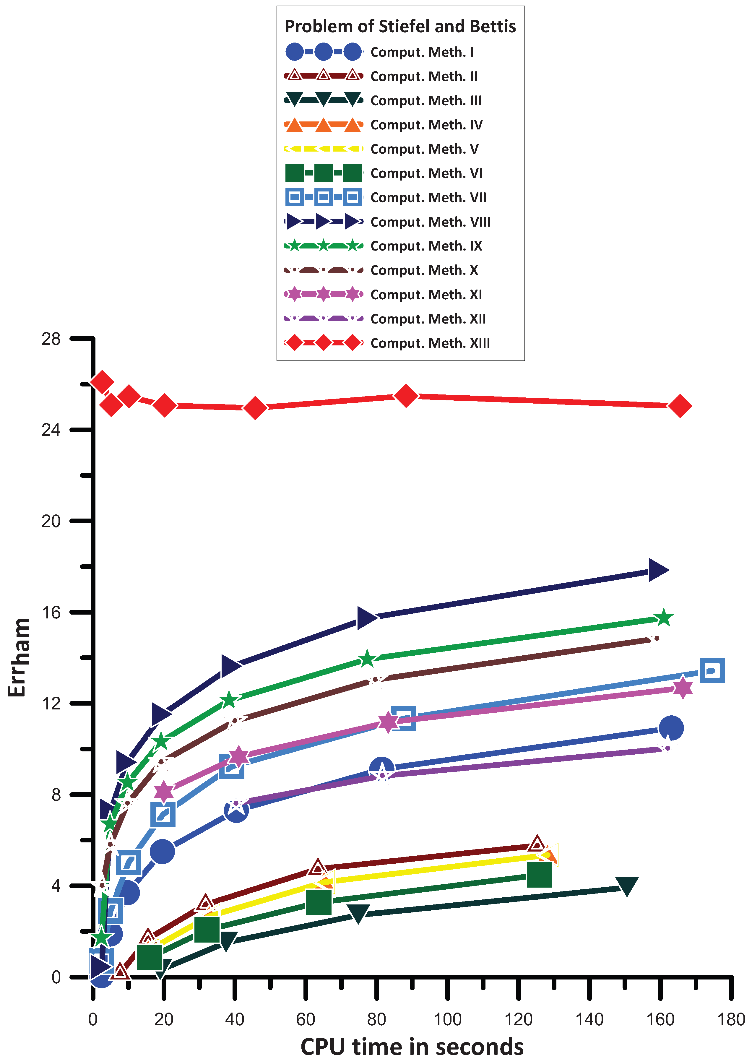
13.1. Problem of Stiefel and Bettis
- The Open Newton–Cotes scheme presented in Section 4 (Classical Case), which is mentioned as Comput. Meth. I;
- The Runge–Kutta Dormand and Prince fourth order method [14], which is mentioned as Comput. Meth. II;
- The Runge–Kutta Dormand and Prince fifth order method [14], which is mentioned as Comput. Meth. III;
- The Runge–Kutta Fehlberg fourth order method [31], which is mentioned as Comput. Meth. IV;
- The Runge–Kutta Fehlberg fifth order method [31], which is mentioned as Comput. Meth. V;
- The Runge–Kutta Cash and Karp fifth order method [32], which is mentioned as Comput. Meth. VI;
- The Amplification-Fitted Open Newton–Cotes scheme with phase lag of order 6, which is developed in Section 5, and which is mentioned as Comput. Meth. VII;
- The Phase-Fitted and Amplification-Fitted Open Newton–Cotes scheme with vanished the first derivative of the amplification factor which is developed in Section 7, and which is mentioned as Comput. Meth. VIII;
- The Phase-Fitted and Amplification-Fitted Open Newton–Cotes scheme with vanished the first derivative of the phase lag which is developed in Section 8, and which is mentioned as Comput. Meth. IX;
- The Phase-Fitted and Amplification-Fitted Open Newton–Cotes scheme which is developed in Section 6, and which is mentioned as Comput. Meth. X;
- The Phase-Fitted and Amplification-Fitted Open Newton–Cotes scheme with vanished the first and second derivatives of the amplification factor which is developed in Section 10, and which is mentioned as Comput. Meth. XI;
- The Phase-Fitted and Amplification-Fitted Open Newton–Cotes scheme with vanished the first and second derivatives of the phase lag which is developed in Section 11, and which is mentioned as Comput. Meth. XII;
- The Phase-Fitted and Amplification-Fitted Open Newton–Cotes scheme with vanished the first derivative of the phase lag and the first derivative of the amplification factor which is developed in Section 9, and which is mentioned as Comput. Meth. XIII.
- Comput. Meth. VI is more efficient than Comput. Meth. III.
- Comput. Meth. IV is more efficient than Comput. Meth. VI.
- Comput. Meth. IV has the same, generally, behavior with Comput. Meth. V.
- Comput. Meth. II is more efficient than Comput. Meth. IV.
- Comput. Meth. XII is more efficient than Comput. Meth. II.
- Comput. Meth. I is more efficient than Comput. Meth. XII for big step sizes and has generally the same behavior with Comput. Meth. XII for small stepsizes.
- Comput. Meth. VII is more efficient than Comput. Meth. I.
- Comput. Meth. XI has the same, generally, behavior with Comput. Meth. VII.
- Comput. Meth. X is more efficient than Comput. Meth. VII.
- Comput. Meth. IX is more efficient than Comput. Meth. X.
- Comput. Meth. VIII is more efficient than Comput. Meth. IX.
- Finally, Comput. Meth. XIII is the most efficient one.
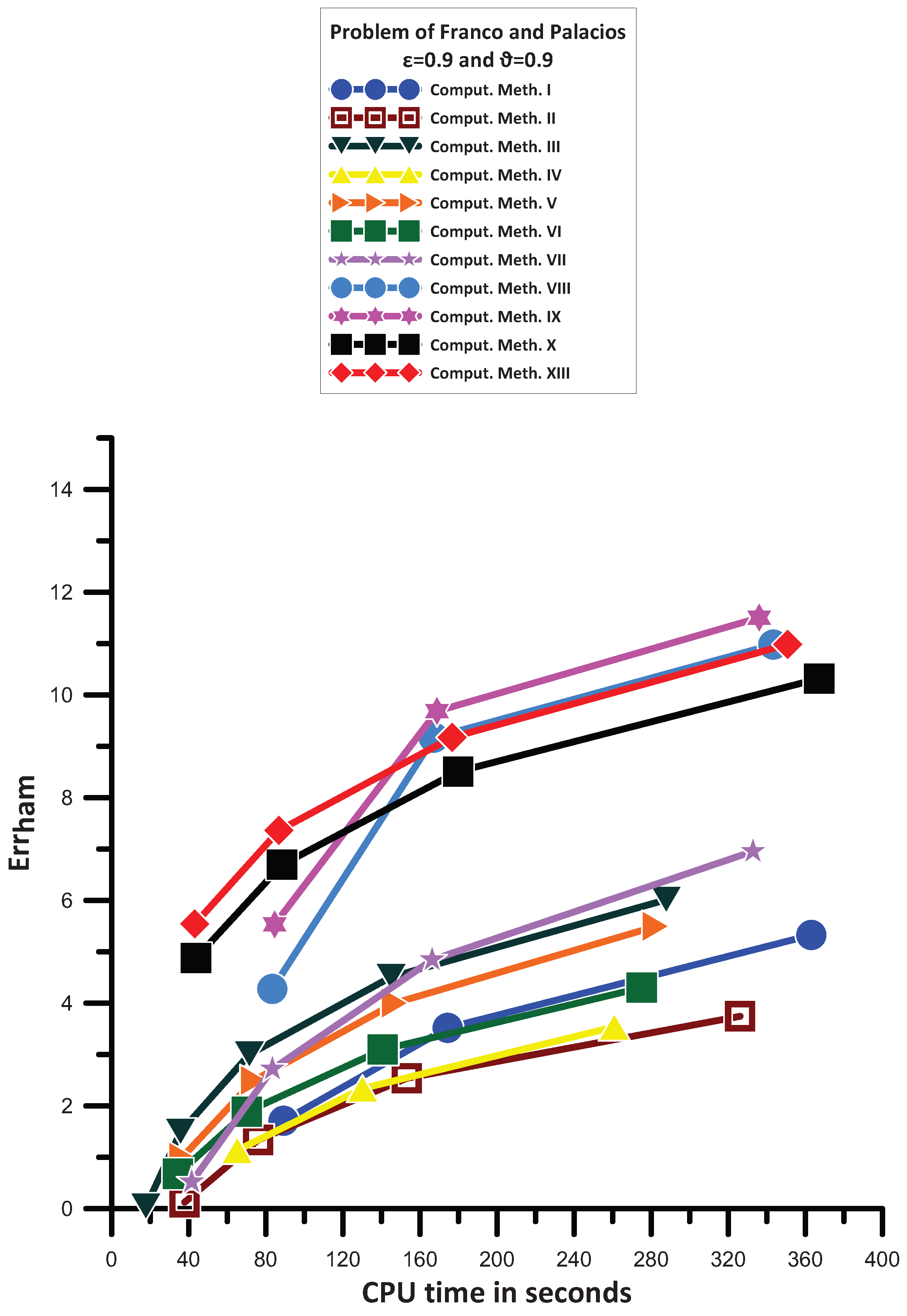
13.2. Problem of Franco and Palacios [33]
- Comput. Meth. XI and Comput. Meth. XII are not convergent for the CPU time used in this example.
- Comput. Meth. II has the same, generally, behavior with Comput. Meth. IV.
- Comput. Meth. I is more efficient than Comput. Meth. II.
- Comput. Meth. VI is more efficient than Comput. Meth. I for big step sizes while for small step sized has the same, generally, behavior.
- Comput. Meth. V is more efficient than Comput. Meth. VI.
- Comput. Meth. III is more efficient than Comput. Meth. V.
- Comput. Meth. VII has a mixed behavior. For big stepsizes is less efficient than Comput. Meth. VI. For medium stepsizes is less efficient than Comput. Meth. III. For small step sizes is more efficient than Comput. Meth. III.
- Comput. Meth. VIII is more efficient than Comput. Meth. III and Comput. Meth. VII.
- Comput. Meth. X is more efficient than Comput. Meth. VIII for big step sizes. For small step sizes Comput. Meth. VIII is more efficient than Comput. Meth. X.
- Comput. Meth. XIII is more efficient than Comput. Meth. X and for small step sizes has the same, generally, behavior with Comput. Meth. VIII.
- Comput. Meth. IX has a mixed behavior. For big stepsizes is less efficient than Comput. Meth. X. For medium stepsizes is less efficient than Comput. Meth. XIII and more efficient than Comput. Meth. X. For small step sizes is the most efficient one.
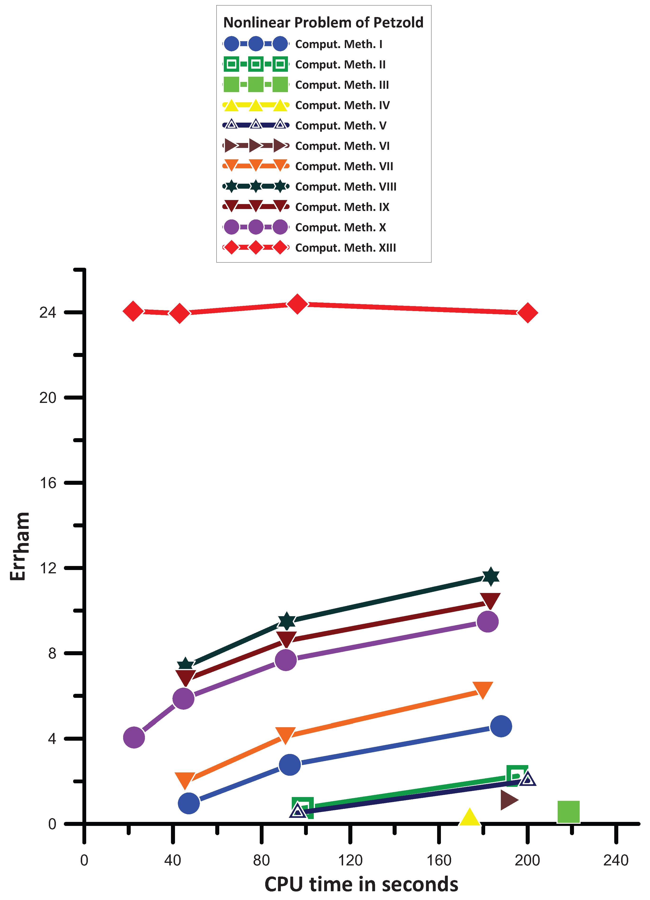
13.3. Nonlinear Problem of Petzold [34]
- Comput. Meth. XI and Comput. Meth. XII are not convergent for the CPU time used in this example.
- Comput. Meth. III has the same, generally, behavior with Comput. Meth. IV.
- Comput. Meth. VI is more efficient than Comput. Meth. III.
- Comput. Meth. V is more efficient than Comput. Meth. VI.
- Comput. Meth. II is more efficient than Comput. Meth. V.
- Comput. Meth. I is more efficient than Comput. Meth. II.
- Comput. Meth. VII is more efficient than Comput. Meth. I.
- Comput. Meth. X is more efficient than Comput. Meth. VII.
- Comput. Meth. IX is more efficient than Comput. Meth. X.
- Comput. Meth. VIII is more efficient than Comput. Meth. IX.
- Finally, Comput. Meth. XIII is the most efficient one.
13.4. A Nonlinear Orbital Problem [35]
- Comput. Meth. XI and Comput. Meth. XII are not convergent for the CPU time used in this example.
- Comput. Meth. VII is more efficient than Comput. Meth. I.
- Comput. Meth. II is more efficient than Comput. Meth. VII.
- Comput. Meth. IV is more efficient than Comput. Meth. II.
- Comput. Meth. VI is more efficient than Comput. Meth. IV.
- Comput. Meth. V is more efficient than Comput. Meth. VI.
- Comput. Meth. III is more efficient than Comput. Meth. V.
- Comput. Meth. VIII is more efficient than Comput. Meth. III.
- Comput. Meth. IX is more efficient than Comput. Meth. VIII.
- Comput. Meth. X has the same, generally, behavior with Comput. Meth. XIII. Finally, Comput. Meth. XIII and Comput. Meth. X are the most efficient ones.

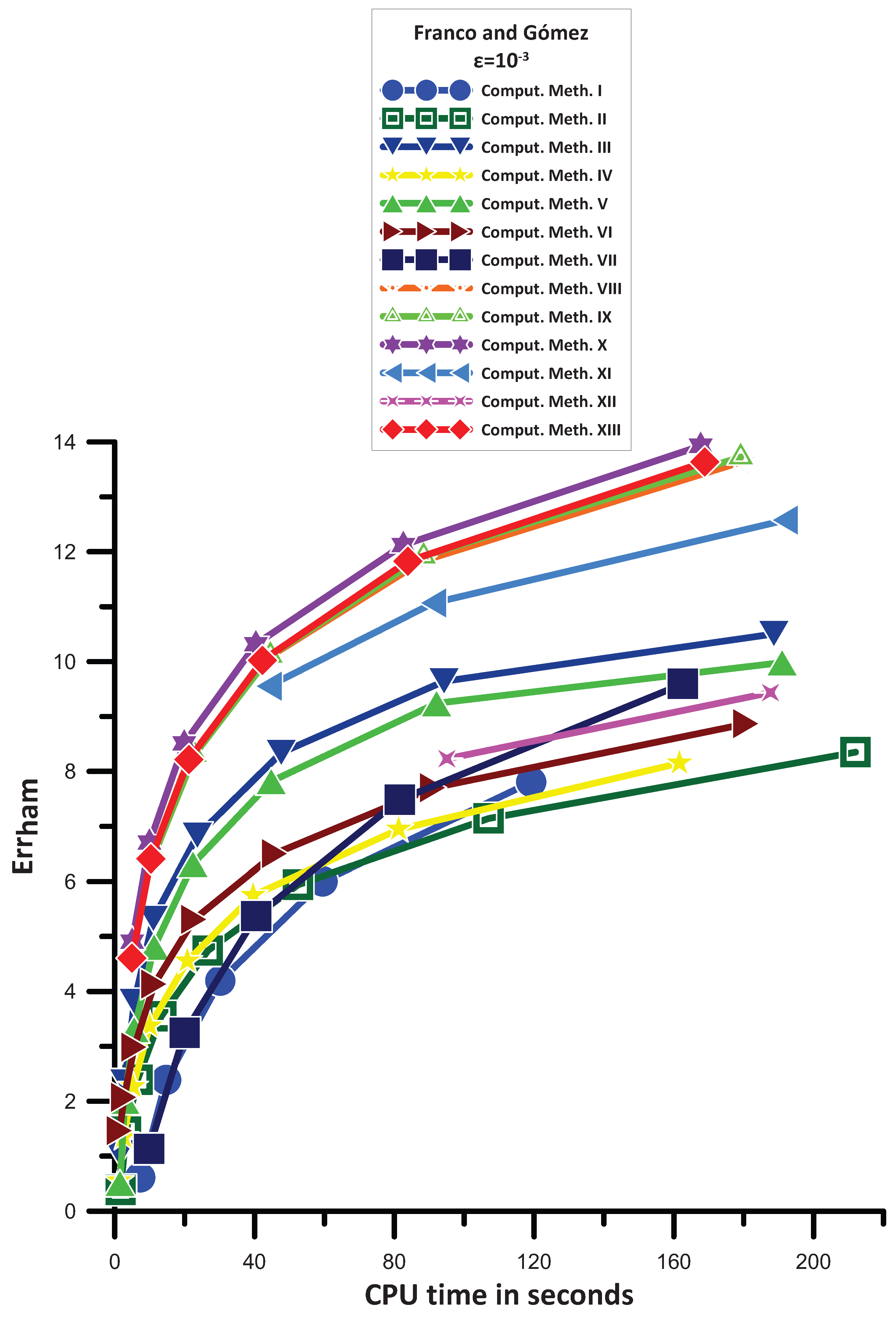
13.5. Problem of Franco and Gómez [36]
- Comput. Meth. II is more efficient than Comput. Meth. I. For small step sizes, Comput. Meth. II is less efficient than Comput. Meth. I.
- Comput. Meth. IV is more efficient than Comput. Meth. II. For small step sizes Comput. Meth. IV is less efficient than Comput. Meth. I.
- Comput. Meth. VII is more efficient than Comput. Meth. IV.
- Comput. Meth. VI is more efficient than Comput. Meth. VII. For small step sizes Comput. Meth. VI is less efficient than Comput. Meth. VII.
- Comput. Meth. XII has a mixed behavior. For bigger stepsizes is more efficient than Comput. Meth. VI and Comput. Meth. VII. For smaller step sizes is less efficient than Comput. Meth. VII and more efficient than Comput. Meth. VI.
- Comput. Meth. V is more efficient than Comput. Meth. VII.
- Comput. Meth. III is more efficient than Comput. Meth. V.
- Comput. Meth. XI is more efficient than Comput. Meth. III.
- Comput. Meth. VIII is more efficient than Comput. Meth. XI.
- Comput. Meth. IX has the same, generally, behavior with Comput. Meth. VIII.
- Comput. Meth. XIII has the same, generally, behavior with Comput. Meth. IX. Consequently, Comput. Meth. VIII, Comput. Meth. IX, and Comput. Meth. XIII have the same, generally, behavior.
- Finally, Comput. Meth. X is the most efficient one.
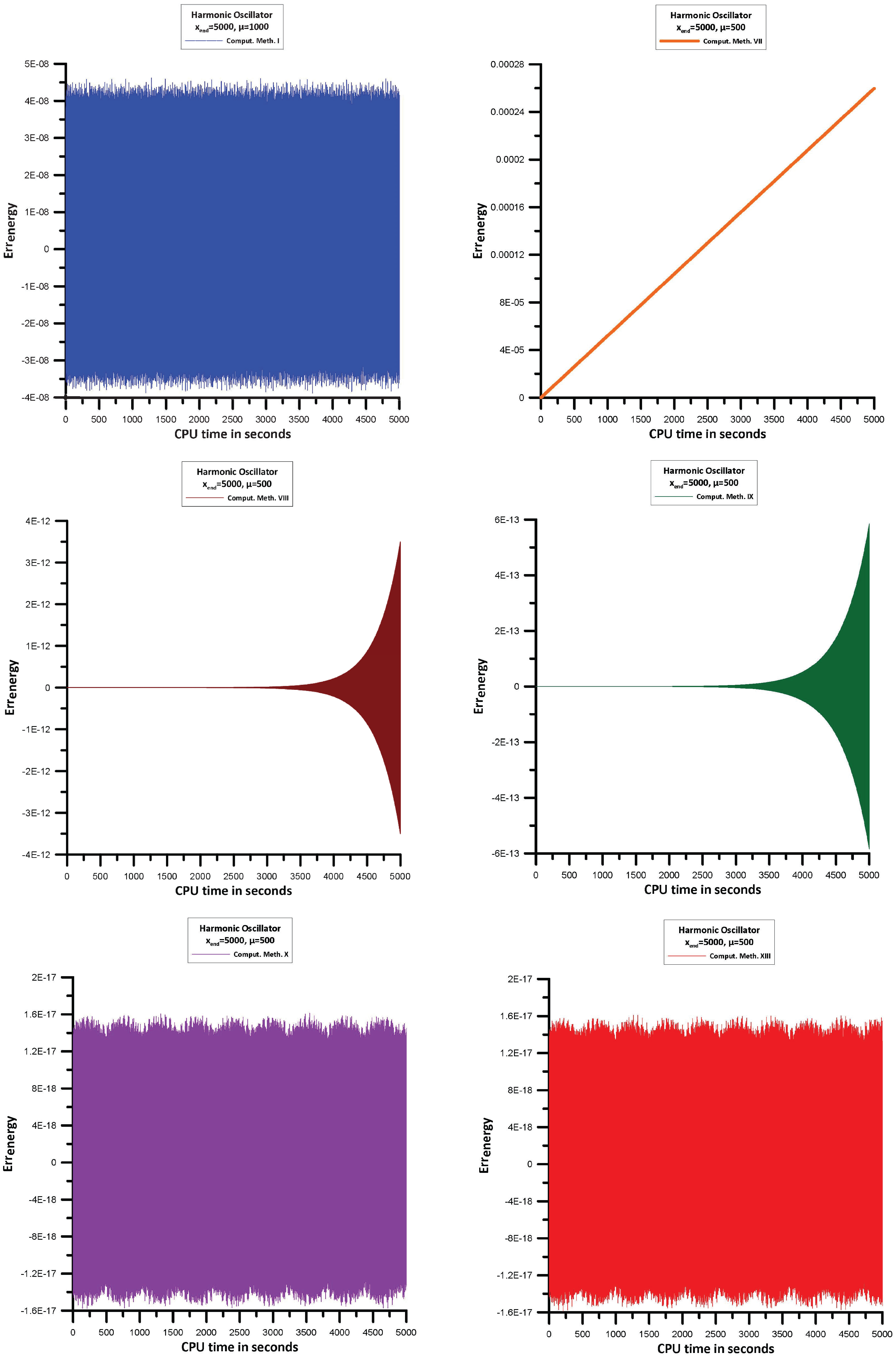
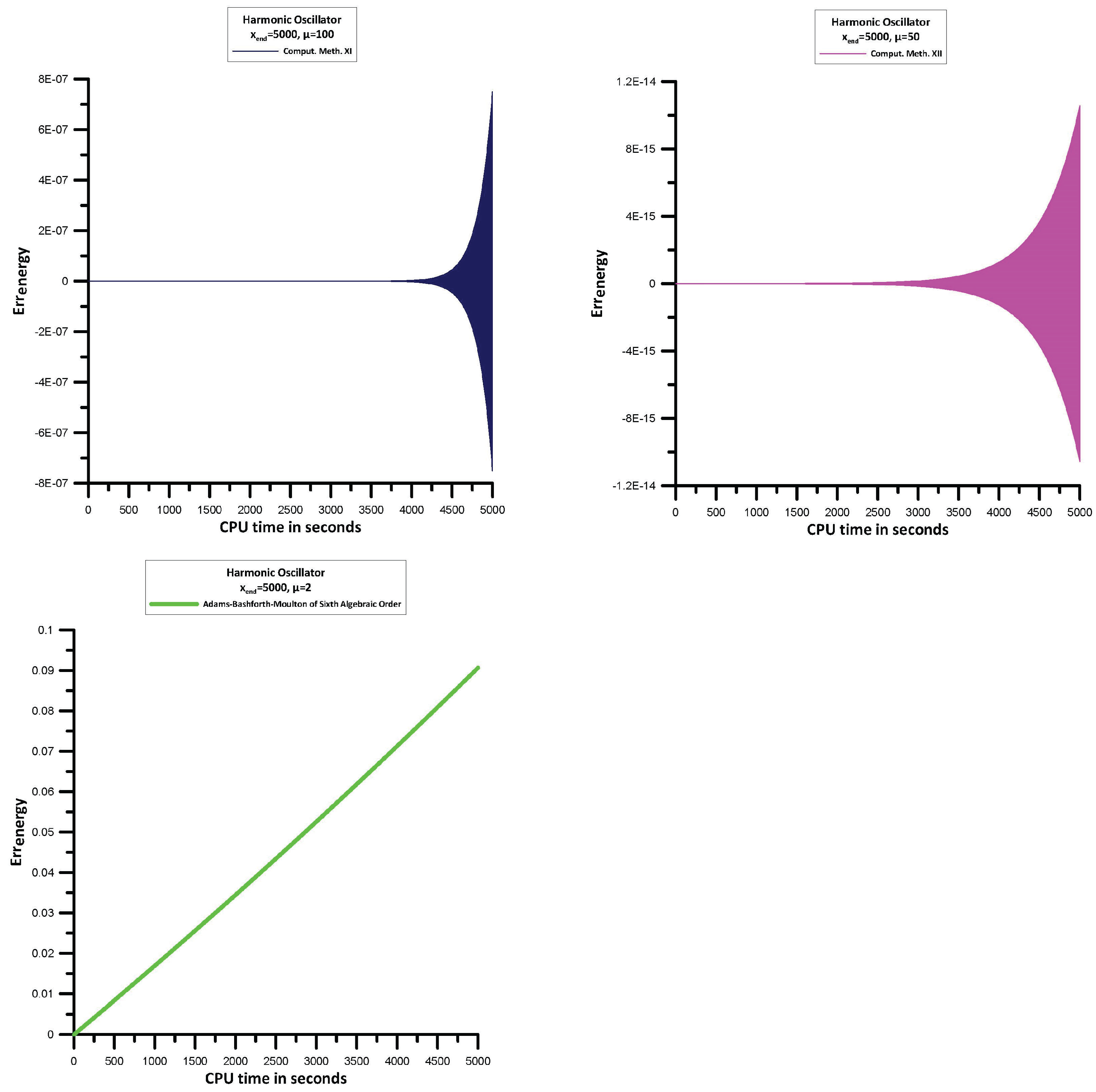
13.6. Hamilton’s Equations of Motion (117)
- Comput. Meth. I, Comput. Meth. VIII, Comput. Meth. IX, Comput. Meth. X, Comput. Meth. XI, Comput. Meth. XII, and Comput. Meth. XIII behave like symplectic integrators.
- From the above methods Comput. Meth. X, and Comput. Meth. XIII are the most efficient ones.
- Comput. Meth. VII is not behave like symplectic integrator and is the less efficient one.
- For comparison purposes we present also the results for the Adams-Bashforth-Moulton sixth algebraic order method which is not behave like symplectic integrator.
13.7. High-Order Ordinary Differential Equations and Partial Differential Equations
13.8. Determination of the Parameter for Every Problem
14. Conclusions
- Strategy for the vanishing of the amplification factor.
- Strategy for the vanishing of the amplification factor and minimization of the phase lag.
- Strategy for the vanishing of the phase lag and vanishing of the amplification factor.
- Strategy for the vanishing of the phase lag and vanishing of the amplification factor together with vanishing of the derivatives of the phase lag.
- Strategy for the vanishing of the phase lag and vanishing of the amplification factor together with vanishing of the derivatives of the amplification factor.
- Strategy for the vanishing of the phase lag and vanishing of the amplification factor together with the vanishing of the derivatives of the phase lag and the vanishing of the amplification factor.
Funding
Data Availability Statement
Conflicts of Interest
Appendix A. Direct Formulae for the Computation of the Derivatives of the Phase Lag and the Amplification Factor
Appendix A.1. Direct Formula for the Derivative of the Phase Lag
Appendix A.2. Direct Formula for the Derivative of the Amplification Factor
Appendix B. Formulae Pari, i = 5(1)7
Appendix C. Formulae Par18, Par19, Par20 and Par21
Appendix D. Formulae Parq, q = 18(1)20
Appendix E. Formulae Parp, p = 22(1)24
Appendix F. Formulae Parν, ν = 25(1)29
Appendix G. Formulae Parμ, μ = 30(1)33
Appendix H. Formulae Parυ, υ = 34(1)40
Appendix I. Formulae Parτ, τ = 41(1)45
Appendix J. Formulae Parφ, φ = 46(1)50
Appendix K. Formulae Parψ, ψ = 51(1)58
Appendix L. Formulae Park, k = 59, 60
References
- Landau, L.D.; Lifshitz, F.M. Quantum Mechanics; Pergamon: New York, NY, USA, 1965. [Google Scholar]
- Prigogine, I.; Rice, S. (Eds.) New Methods in Computational Quantum Mechanics. In Advances in Chemical Physics; John Wiley & Sons: Hoboken, NJ, USA, 1997; Volume 93. [Google Scholar]
- Simos, T.E. Numerical Solution of Ordinary Differential Equations with Periodical Solution. Doctoral Dissertation, National Technical University of Athens, Athens, Greece, 1990. (In Greek). [Google Scholar]
- Ixaru, L.G. Numerical Methods for Differential Equations and Applications; Reidel: Dordrecht, The Netherlands; Boston, MA, USA; Lancaster, UK, 1984. [Google Scholar]
- Quinlan, G.D.; Tremaine, S. Symmetric multistep methods for the numerical integration of planetary orbits. Astron. J. 1990, 100, 1694–1700. [Google Scholar] [CrossRef]
- Lyche, T. Chebyshevian multistep methods for ordinary differential equations. Numer. Math. 1972, 10, 65–75. [Google Scholar] [CrossRef]
- Konguetsof, A.; Simos, T.E. On the construction of Exponentially Fitted Methods for the Numerical Solution of the Schrödinger Equation. J. Comput. Meth. Sci. Eng. 2001, 1, 143–165. [Google Scholar] [CrossRef]
- Dormand, J.R.; El-Mikkawy, M.E.A.; Prince, P.J. Families of Runge–Kutta-Nyström formulae. IMA J. Numer. Anal. 1987, 7, 235–250. [Google Scholar] [CrossRef]
- Franco, J.M.; Gomez, I. Some procedures for the construction of high-order exponentially fitted Runge–Kutta-Nyström Methods of explicit type. Comput. Phys. Commun. 2013, 184, 1310–1321. [Google Scholar] [CrossRef]
- Franco, J.M.; Gomez, I. Accuracy and linear Stability of RKN Methods for solving second-order stiff problems. Appl. Numer. Math. 2009, 59, 959–975. [Google Scholar] [CrossRef]
- Chien, L.K.; Senu, N.; Ahmadian, A.; Ibrahim, S.N.I. Efficient Frequency-Dependent Coefficients of Explicit Improved Two-Derivative Runge–Kutta Type Methods for Solving Third- Order IVPs. Pertanika J. Sci. Technol. 2023, 31, 843–873. [Google Scholar] [CrossRef]
- Zhai, W.J.; Fu, S.H.; Zhou, T.C.; Xiu, C. Exponentially fitted and trigonometrically fitted implicit RKN methods for solving y" = f (t, y). J. Appl. Math. Comput. 2022, 68, 1449–1466. [Google Scholar] [CrossRef]
- Fang, Y.L.; Yang, Y.P.; You, X. An explicit trigonometrically fitted Runge–Kutta method for stiff and oscillatory problems with two frequencies. Int. J. Comput. Math. 2020, 97, 85–94. [Google Scholar] [CrossRef]
- Dormand, J.R.; Prince, P.J. A family of embedded Runge–Kutta formulae. J. Comput. Appl. Math. 1980, 6, 19–26. [Google Scholar] [CrossRef]
- Chawla, M.M.; Rao, P.S. A Noumerov-Type Method with Minimal Phase-Lag for the Integration of 2nd Order Periodic Initial-Value Problems. J. Comput. Appl. Math. 1984, 11, 277–281. [Google Scholar] [CrossRef]
- Ixaru, L.G.; Rizea, M. A Numerov-like scheme for the numerical solution of the Schrödinger equation in the deep continuum spectrum of energies. Comput. Phys. Commun. 1980, 19, 23–27. [Google Scholar] [CrossRef]
- Raptis, A.D.; Allison, A.C. Exponential-fitting Methods for the numerical solution of the Schrödinger equation. Comput. Phys. Commun. 1978, 14, 1–5. [Google Scholar] [CrossRef]
- Wang, Z.; Zhao, D.; Dai, Y.; Wu, D. An improved trigonometrically fitted P-stable Obrechkoff Method for periodic initial-value problems. Proc. R. Soc.-Math. Phys. Eng. Sci. 2005, 461, 1639–1658. [Google Scholar]
- Wang, C.; Wang, Z. A P-stable eighteenth-order six-Step Method for periodic initial value problems. Int. J. Mod. Phys. 2007, 18, 419–431. [Google Scholar] [CrossRef]
- Shokri, A.; Khalsaraei, M.M. A new family of explicit linear two-step singularly P-stable Obrechkoff methods for the numerical solution of second-order IVPs. Appl. Math. Comput. 2020, 376, 125116. [Google Scholar] [CrossRef]
- Abdulganiy, R.I.; Ramos, H.; Okunuga, S.A.; Majid, Z.A. A trigonometrically fitted intra-step block Falkner method for the direct integration of second-order delay differential equations with oscillatory solutions. Afr. Mat. 2023, 34, 36. [Google Scholar] [CrossRef]
- Lee, K.C.; Senu, N.; Ahmadian, A.; Ibrahim, S.N.I. High-order exponentially fitted and trigonometrically fitted explicit two-derivative Runge–Kutta-type methods for solving third-order oscillatory problems. Math. Sci. 2022, 16, 281–297. [Google Scholar] [CrossRef]
- Fang, Y.L.; Huang, T.; You, X.; Zheng, J.; Wang, B. Two-frequency trigonometrically fitted and symmetric linear multi-step methods for second-order oscillators. J. Comput. Appl. Math. 2021, 392, 113312. [Google Scholar] [CrossRef]
- Chun, C.; Neta, B. Trigonometrically Fitted Methods: A Review. Mathematics 2019, 7, 1197. [Google Scholar] [CrossRef]
- Simos, T.E. A New Methodology for the Development of Efficient Multistep Methods for First-Order IVPs with Oscillating Solutions. Mathematics 2024, 12, 504. [Google Scholar] [CrossRef]
- Simos, T.E. A New Methodology for the Development of Efficient Multistep Methods for First-Order IVPs with Oscillating Solutions IV: The Case of the Backward Differentiation Formulae. Axioms 2024, 13, 649. [Google Scholar] [CrossRef]
- Saadat, H.; Kiyadeh, S.H.H.; Karim, R.G.; Safaie, A. Family of phase fitted 3-step second-order BDF methods for solving periodic and orbital quantum chemistry problems. J. Math. Chem. 2024, 62, 1223–1250. [Google Scholar] [CrossRef]
- Saadat, H.; Kiyadeh, S.H.H.; Safaie, A.; Karim, R.G.; Khodadosti, F. A new amplification-fitting approach in Newton–Cotes rules to tackling the high-frequency IVPs. Appl. Numer. Math. 2025, 207, 86–96. [Google Scholar] [CrossRef]
- Zhu, W.; Zhao, X.; Tang, Y. Numerical methods with a high order of accuracy applied in the quantum system. J. Chem. Phys. 1996, 104, 2275–2286. [Google Scholar] [CrossRef]
- Stiefel, E.; Bettis, D.G. Stabilization of Cowell’s Method. Numer. Math. 1969, 13, 154–175. [Google Scholar] [CrossRef]
- Fehlberg, E. Classical Fifth-, Sixth-, Seventh-, and Eighth-Order Runge–Kutta Formulas with Stepsize Control; NASA Technical Report 287; NASA: Washington, DC, USA, 1968. Available online: https://ntrs.nasa.gov/api/citations/19680027281/downloads/19680027281.pdf (accessed on 10 December 1997).
- Cash, J.R.; Karp, A.H. A variable order Runge–Kutta method for initial value problems with rapidly varying right-hand sides. ACM Trans. Math. Softw. 1990, 16, 201–222. [Google Scholar] [CrossRef]
- Franco, J.M.; Palacios, M. High-order P-stable multistep methods. J. Comput. Appl. Math. 1990, 30, 1–10. [Google Scholar] [CrossRef]
- Petzold, L.R. An efficient numerical method for highly oscillatory ordinary differential equations. SIAM J. Numer. Anal. 1981, 18, 455–479. [Google Scholar] [CrossRef]
- Simos, T.E. New Open Modified Newton Cotes Type Formulae as Multilayer Symplectic Integrators. Appl. Math. Model. 2013, 37, 1983–1991. [Google Scholar] [CrossRef]
- Franco, J.; Gómez, I. Trigonometrically fitted nonuliear two-step methods for solving second order oscillatory IVPs. Appl. Math. Comput. 2014, 232, 643–657. [Google Scholar]
- Boyce, W.E.; DiPrima, R.C.; Meade, D.B. Elementary Differential Equations and Boundary Value Problems, 11th ed.; John Wiley & Sons: Hoboken, NJ, USA, 2017. [Google Scholar]
- Evans, L.C. Partial Differential Equations: Second Edition; American Mathematical Society: Providence, RI, USA, 2010; Chapter 3; pp. 91–135. [Google Scholar]
- Ramos, H.; Vigo-Aguiar, J. On the frequency choice in trigonometrically fitted methods. Appl. Math. Lett. 2010, 23, 1378–1381. [Google Scholar] [CrossRef]
- Ixaru, L.G.; Berghe, G.V.; Meyer, H.D. Frequency evaluation in exponential fitting multistep algorithms for ODEs. J. Comput. Appl. Math. 2002, 140, 423–434. [Google Scholar] [CrossRef]
Disclaimer/Publisher’s Note: The statements, opinions and data contained in all publications are solely those of the individual author(s) and contributor(s) and not of MDPI and/or the editor(s). MDPI and/or the editor(s) disclaim responsibility for any injury to people or property resulting from any ideas, methods, instructions or products referred to in the content. |
© 2024 by the author. Licensee MDPI, Basel, Switzerland. This article is an open access article distributed under the terms and conditions of the Creative Commons Attribution (CC BY) license (https://creativecommons.org/licenses/by/4.0/).
Share and Cite
Simos, T.E. A New Methodology for the Development of Efficient Multistep Methods for First-Order Initial Value Problems with Oscillating Solutions V: The Case of the Open Newton–Cotes Differential Formulae. Mathematics 2024, 12, 3652. https://doi.org/10.3390/math12233652
Simos TE. A New Methodology for the Development of Efficient Multistep Methods for First-Order Initial Value Problems with Oscillating Solutions V: The Case of the Open Newton–Cotes Differential Formulae. Mathematics. 2024; 12(23):3652. https://doi.org/10.3390/math12233652
Chicago/Turabian StyleSimos, Theodore E. 2024. "A New Methodology for the Development of Efficient Multistep Methods for First-Order Initial Value Problems with Oscillating Solutions V: The Case of the Open Newton–Cotes Differential Formulae" Mathematics 12, no. 23: 3652. https://doi.org/10.3390/math12233652
APA StyleSimos, T. E. (2024). A New Methodology for the Development of Efficient Multistep Methods for First-Order Initial Value Problems with Oscillating Solutions V: The Case of the Open Newton–Cotes Differential Formulae. Mathematics, 12(23), 3652. https://doi.org/10.3390/math12233652