A Nonconvex Approach with Structural Priors for Restoring Underwater Images

Abstract

Underwater image restoration is a crucial task in various computer vision applications, including underwater target detection and recognition, autonomous underwater vehicles, underwater rescue, marine organism monitoring, and marine geological survey. Among other categories, the physics-based methods restore underwater images by improving the transmission map through optimization or regularization techniques. Conventional optimization-based methods often do not consider the effect of structural differences between guidance and transmission maps. To address this issue, in this paper, we present a regularization-based method for restoring underwater images that uses coherent structures between the guidance map and the transmission map. The proposed approach models the optimization of transmission maps through a nonconvex energy function comprising data and smoothness terms. The smoothness term includes static and dynamic structural priors, and the optimization problem is solved using a majorize-minimize algorithm. We evaluate the proposed method on benchmark datasets, and the results demonstrate the superiority of the proposed method over state-of-the-art techniques in terms of improving transmission maps and producing high-quality restored images.

1. Introduction

Restoration of underwater images is a crucial task in improving the underwater environment, with applications in various domains such as underwater target detection and recognition, autonomous underwater vehicles, search and rescue operations, monitoring of sea organisms, and marine geological surveying [1]. However, the acquisition of underwater optical imaging suffers from several degradation factors such as strong light absorption, light scattering and attenuation, color distortion, and noise from artificial light sources. The attenuation of light depends both on distances of the device to the object and the light’s wavelengths. In addition, underwater imaging is also exaggerated by seasonal, geographic, and climate variations [2,3]. These factors, in turn, severely affect the quality of the captured images, and the image restoration becomes a challenging task.

In literature, underwater image restoration and dehazing are well-studied, and numerous methods have been proposed [4,5,6,7,8,9,10,11,12]. Among these methods, hardware-based techniques [4,5] use multiple images or polarization imaging to enhance the visibility of underwater images. However, the complexity of such devices posed difficulties in capturing image sequences. More recently, restoration-based methods [6,13] have been proposed, but they often face challenges in accurately estimating the parameters of underwater imaging models. Similarly, enhancement-based methods [10,11] can improve the contrast and brightness of underwater images, but they may introduce over-enhancement and over-saturation problems. Learning-based methods [12,14] have also been explored; however, the scarcity of high-quality training images remains a significant challenge. A variety of optimization-based methods [15,16,17] recover images with reasonable accuracy. Mostly, these methods adopt the model proposed in Schechner and Kopeika [18], estimate initial transmission map (TM) through various prior [19,20,21,22,23], and then optimize TM by utilizing weights from some guidance image. However, these methods do not incorporate the structural differences between TM and the guidance map. Consequently, images recovered are of poor quality.

In this paper, an underwater image restoration method is proposed that incorporates the utilization of a robust regularization of coherent structures in the image and transmission map. A primary study of this method with limited results is presented in [17]. The proposed method takes into consideration the potential structural differences between the transmission map and the guidance map. The problem of optimization of the transmission map is modeled through a nonconvex energy function, which consists of data and smoothness terms. The algorithm is further solved using a majorize-minimize (MM) [24,25] approach. The proposed method is tested on a benchmark dataset [3], and its performance is compared to the state-of-the-art methods, which indicates that the proposed method performs well and achieves improved results in restoring high-quality images. The rest of the paper is organized as:

• In Section 2, the background and the related work to the underwater image restoration is explained. Moreover, the image degradation in water is also explained using the atmospheric scattering model (ASM).
• Section 3 describes the proposed method in detail. First, the initial transmission map is computed, and then an energy function is suggested to improve the initial transmission map. The optimization of the energy function using the surrogate function and the majorize-minimize algorithm is also explained.
• In Section 4, the experimental setup and results are provided. Ablation study and the comparative analysis are presented for the evaluation of the performance of the proposed method
• Finally, the study is concluded in Section 5.

2. Related Work

2.1. Atmospheric Scattering Model

Usually, the atmospheric scattering model (ASM) is used to describe the degradation of images when light rays scatter through the medium, such as water, air, fog, cloud, and rain, etc. The underwater image formation is depicted in Figure 1, where it can be observed that the image-capturing device receives three types of light: (1) the reflected light comes to the camera directly after striking the object, (2) the forward-scattered light that deviates from its way from the original direction after striking the object, and (3) the backscattering light comes to the camera after encountering particles. According to Koschmieder’s law [26], only a proportion of reflected light reaches the camera, leading to poor visibility in aquatic environments. There are various image formation methods that describe the formation of images in scattering media, but we adopt the ASM model proposed in Schechner and Kopeika [18] in this work. According to this model, the intensity of the image at each pixel is composed of two components: the attenuated intensity, which represents the amount of light reflected by the object and captured by the camera through the medium, and the veiling light, which represents the light scattered by the medium. Thus, the degraded image is the combination of the attenuated and scattered light captured through the image-capturing device. The model can be represented as

$$I\left(\mathit{x}\right)=J\left(\mathit{x}\right)t\left(\mathit{x}\right)+A(1-t(\mathit{x}\left)\right),$$

(1)

where,

Figure 1. Formation of underwater images. The direct transmission of light contains valuable information about the scene, while the backscattered light degrades the image by reflecting off the suspended particles in the water column. The distance between the camera and the object, denoted by z, affects the clarity of the image. Red light is absorbed more quickly than other wavelengths, making it less effective for underwater imaging. Additionally, forward scattered light can blur the scene, further reducing image quality.

• $\mathit{x}$ denotes the pixel coordinates,
• $I\left(\mathit{x}\right)$ is the captured degraded image,
• $J\left(\mathit{x}\right)$ is the object radiance, i.e., the clear image or the target image,
• $t\left(\mathit{x}\right)$ is the transmission map,
• A is the global atmospheric light or (Veiling light).

In other words, in the resultant image $I\left(\mathit{x}\right)$, the attenuated intensity $\left\{J\right(\mathit{x}\left)t\right(\mathit{x}\left)\right\}$, and the atmospheric intensity $\left\{A\right(1-t\left(\mathit{x}\right)\left)\right\}$ are combined. Both types of intensities depend on the medium through which light travels. In a more formal way, $I(.)$ and $t(.)$ are mappings from the domain $\mathsf{\Omega }$ to a range V, i.e., $I(.),t(.):\mathsf{\Omega }\mapsto V$, then each element $\mathit{x}\in \mathsf{\Omega }$ is mapped onto values $I\left(\mathit{x}\right)\in V,t\left(\mathit{x}\right)\in V$. So values from V are positive real numbers, and $\mathsf{\Omega }$ is the pixel position in the 2D grid of the image size, i.e., two positive integers within the image size represent the location of the pixel. In homogeneous media, the transmission map (TM) can be described by

$$t\left(\mathit{x}\right)=e^{-\beta z\left(\mathit{x}\right)},$$

(2)

where $\beta$ is the medium attenuation coefficient and $z\left(\mathit{x}\right)$ is the depth or distance of the object from the camera. The primary objective of underwater image restoration methods is to recover the original image $J\left(\mathit{x}\right)$, the atmospheric light A, and the transmission map $t\left(\mathit{x}\right)$ from the observed image $I\left(\mathit{x}\right)$. Methods for underwater images can roughly be divided into various categories, including physics-based models, non-physics-based models, specialized hardware-based models, and deep-learning-based model methods.

2.2. Physics-Based Methods

Typically, physics-based methods restore the image in two steps. In the first step, an initial transmission map is computed. Usually, an initial transmission map is estimated using various man-made priors. In literature, various priors include Dark Channel Prior [26], underwater Dark Channel Prior [19], minimum information loss and HDP [20], blurriness prior [27], attenuation curve prior [28], general dark channel prior [29], haze lines prior [30] underwater haze lines prior [3], red channel prior [21], bright channel prior [22] are used to compute the initial transmission map. In the second step, the initial transmission maps are refined. After that, the model is inverted to generate a clear image by using atmospheric light and the refined transmission map. For enhancing transmission maps, various techniques, such as guided filter (GF) [31], mutual structure filtering (MSF) [32], soft matting [26], and static dynamic filtering (SDF) [25]. In a single-image-de-hazing method [26], minimum channel values in a small window are considered as the estimation of transmission map, and then a guided filter [31] is used for the refinement of the initial map. In [19], a method is proposed based on Dark Channel Prior, called Underwater DCP, to estimate the transmission map in underwater single images, considering the blue and green color channels and discarding the red channel.

2.3. Non-Physics Based Methods

Non-physics-based methods: Generally, these methods involve directly modifying an image’s pixel value to enhance the visual appeal of underwater images. Representative methods include the Retinex-based methods [33], histogram stretching methods [34], and image fusion methods [35,36]. For example, Ancuti et al. [36] provided a multi-scale approach and used it to combine the contrast and color-enhanced versions produced by a white-balancing technique. These non-physics-based methods can enhance the color and contrast of underwater photos, but they are blind to the underwater imaging models. As a result, the improved images are over-enhanced and over-saturated. In addition, there are a few effective hardware-based methods, including the range-gated imaging [37], polarization de-scattering imaging [38], or free-ascending deep-sea tripods [39] to improve the visual quality of underwater images. However, it is challenging for hardware devices to collect image sequences of the same scene. In CIEV [40], the underwater image restoration problem is formulated as an energy function that consists of the contrast term and the information loss term. By minimizing this energy function, the contrast is enhanced and the color information is preserved optimally. In another work, Zhang et al. [41] introduced an MMLE model to deal with degraded underwater images via the locally adaptive color correction method (LACC) and locally adaptive contrast enhancement (LACE). In addition, Jun Xie et al. [42] proposed the UNTV method to compute noise captured through forwarding signals using UIFM. These physics-based methods, in general, are effective in some cases but do not produce satisfactory results when it comes to different optical properties of water due to their heavy reliance on man-made priors.

2.4. Deep-Learning-Based Methods

In the field of underwater image enhancement and restoration, deep learning methods have gained popularity in recent years. For instance, Ye et al. [14] introduced an unsupervised adaptation network in 2020 that employed style-level and feature-level adaptation to achieve domain invariance. Additionally, Ye et al. developed a task network to estimate scene depth. Wang et al. [43] proposed a convolutional-neural-network-(CNN)-based end-to-end framework for color correction and haze removal, which included a pixel-disrupting strategy to improve convergence speed and accuracy. While the CNN-based approach performed well in enhancing brightness and contrast, it tended to over-enhance red tones. Li et al. [44] created a convolutional network model with dense connectivity for underwater image and video enhancement, which relied on the prior knowledge of underwater scenes to directly recover clear images without estimating the transmission and backscatter. Yang et al. [45] designed a conditional generative adversarial network (cGAN) to reconstruct latent underwater images using a multi-scale generator and dual discriminator. While deep learning methods can achieve good results in certain underwater scenarios, it is impractical to use a single trained network for all types of underwater images due to the complexity and variability of the underwater imaging environment. Transformer-based networks like DehazeFormer by Song et al. [46] make significant modifications in traditional structures and employ innovative techniques like SoftReLU and RescaleNorm, presenting better performance in dehazing tasks with efficient computational cost and parameter utilization. In a more recent deep-learning-based method [47], a style transfer network is used to synthesize underwater images from clear images. Then an underwater image enhancement network with a U-shaped convolutional variational autoencoder is constructed for underwater image restoration. In [48], an underwater image enhancement scheme is proposed that incorporates domain adaptation. Firstly, an underwater dataset fitting model (UDFM) is developed for merging degraded datasets. Then an underwater image enhancement model (UIEM) is suggested for image enhancement. In a more recent work [49], we propose a multi-task fusion where fusion weights are obtained from the similarity measures. Fusion based on such weights provides better image enhancement and restoration capabilities.

3. Proposed Method

The proposed method for the underwater image restoration consists of mainly three steps, as illustrated in Figure 2. The first step involves the computing of the initial transmission map (TM). In the second step, the initial TM is refined through the proposed nonconvex energy framework, which involves the computation of static and dynamic weights from the input image and the iterative regularization of the transmission estimate. In the final step, the image is restored using the ASM (Equation (1)). Detailed descriptions of these steps are provided in the subsequent sections.

Figure 2. Outlines of the proposed method. Following the physical scattering model, initial TM and veiling light are computed from the input image. Then the initial TM is refined by solving a robust energy function that takes advantage of a non-convex regularizer and two types of weights. Finally, the image is restored using the refined TM and the ASM.

3.1. Initial Transmission Map

In the literature, difference priors are used to estimate the transmission map. In our method, we have used the haze-lines (HL) prior for this purpose [3]. First, the veiling light A is computed by the the average color of 20% pixels that are belonging to the largest component from the edge map of the input image $I\left(\mathit{x}\right)$. Then, according to the HL prior-based transmission map estimation method, the translated RGB coordinate system at the origin can be expressed as

$$I_A\left(\mathit{x}\right)=t\left(\mathit{x}\right)J_A\left(\mathit{x}\right),$$

(3)

where,

$$\begin{array}{cc}\hfill I_A\left(\mathit{x}\right)& \hfill =I\left(\mathit{x}\right)-A,\hfill \end{array}$$

(4)

$$\begin{array}{cc}\hfill J_A\left(\mathit{x}\right)& \hfill =J\left(\mathit{x}\right)-A.\hfill \end{array}$$

(5)

Further, $I_A\left(\mathit{x}\right)$ can be written using spherical coordinates as

$$I_A\left(\mathit{x}\right)=[r\left(\mathit{x}\right),\theta \left(\mathit{x}\right),\varphi \left(\mathit{x}\right)]$$

(6)

where $r\left(\mathit{x}\right)$ is the distance to the origin, and $\theta \left(\mathit{x}\right)$ and $\varphi \left(\mathit{x}\right)$ are the angles with longitude and latitude, respectively [3]. The initial transmission map $t\left(\mathit{x}\right)$ is computed as;

$$t\left(\mathit{x}\right)={\displaystyle \frac{r\left(\mathit{x}\right)}{r_{max}}},$$

(7)

where $r_{max}$ is the maximum distance of haze-line from the origin. For a haze-line, this maximum value occurs at the haze-free pixel which is the farthest pixel from A. Therefore, $r_{max}=\parallel J_A\left(\mathit{x}\right)\parallel$ is the maximum distance of that haze-line.

The initial transmission map $t\left(\mathit{x}\right)$ is computed per pixel and not consistent between nearby pixels. Thus inaccuracies in tranmission map results in poor restoration. To improve this initial transmission map $t\left(\mathit{x}\right)$, we propose the use of non-convex regularization. This improvement in transmission map ultimately leads to the restoration of higher-quality images.

3.2. Model

We propose the improvement of the initial transmission map $t\left(\mathit{x}\right)$ by efficiently minimizing the following energy function.

$$\mathcal{E}\left(\widehat{t}\left(\mathit{x}\right)\right)=\sum _{\mathit{x}\in \mathsf{\Omega }}{\left(\widehat{t}\left(\mathit{x}\right)-t\left(\mathit{x}\right)\right)}^2+\lambda \mathsf{\Theta }\left(\widehat{t}\left(\mathit{x}\right)\right),$$

(8)

where,

• $t\left(\mathit{x}\right)$ is the initial transmission map,
• $\widehat{t}\left(\mathit{x}\right)$ is the regularized or estimated transmission map,
• is the first term on the right-hand side ${\left(\widehat{t}\left(\mathit{x}\right),t\left(\mathit{x}\right)\right)}^2$ is the data fidelity term,
• is the second term on the right-hand side $\mathsf{\Theta }\left(\widehat{t}\left(\mathit{x}\right)\right)$, is the regularization term,
• $\lambda$ is the constant that determines the significance of these two terms, and
• $\mathsf{\Omega }$ is the domain for transmission map, i.e., represents the pixel positions in the 2D grid of the image size.

In our case, the following regularizer is proposed

$$\mathsf{\Theta }\left(\widehat{t}\left(\mathit{x}\right)\right)=\sum _{\mathit{x}\in \mathsf{\Omega }}\sum _{\mathit{y}\in {\mathcal{N}}_{\mathit{x}}}{w}_{\mathit{x},\mathit{y}}\left(g\left(\mathit{x}\right)\right){\varphi }_{\gamma }\left(\widehat{t}\left(\mathit{x}\right)-\widehat{t}\left(\mathit{y}\right)\right),$$

(9)

where,

• ${\mathcal{N}}_{\mathit{x}}$ is a small 2D local neighborhood window centered at $\mathit{x}$,
• $\mathit{y}\in {\mathcal{N}}_{\mathit{x}}$ is a pixel in the neighborhood of pixel $\mathit{x}$,
• $w_{\mathit{x},\mathit{y}}(.)$ is the spatially varying weighting function,
• $g\left(\mathit{x}\right)$ is the pixel-wise guidance. In our case, the gray-scale image computed from the input image $I\left(\mathit{x}\right)$ has been taken as the guidance $g\left(\mathit{x}\right)$.
• The function ${\varphi }_{\gamma }(.)$ computes the neighborhood coherence by taking the difference between the estimated TM values at a pixel location $\mathit{x}$ and its neighbor $\mathit{y}$.

The spatially varying weights (also named static guidance or static weights) for each pixel location are computed as

$$w_{\mathit{x},\mathit{y}}\left(g\left(\mathit{x}\right)\right)=exp\left(-{\alpha }_1{(\mathit{x}-\mathit{y})}^2\right)exp\left(-{\alpha }_2{\left(g\left(\mathit{x}\right)-g\left(\mathit{y}\right)\right)}^2\right),$$

(10)

where the first term is the spatial filter, the second is the intensity range filter, and ${\alpha }_1$ and ${\alpha }_2$ are the positive parameters defined by the user. These parameters control the regularization (smoothness) effect. These guidance weights are static, as they are computed once and used in each iteration during the optimization process.

The second factor term in the regularizer is parameterized through the square hyperbolic tangent function, which is given by

$${\varphi }_{\gamma }\left(\widehat{t}\left(\mathit{x}\right)-\widehat{t}\left(\mathit{y}\right)\right)=tanh\left(\gamma {\left(\widehat{t}\left(\mathit{x}\right)-\widehat{t}\left(\mathit{y}\right)\right)}^2\right),$$

(11)

where $\gamma$ is a positive parameter that controls the steepness of this function. It maps the difference between $\widehat{t}\left(\mathit{x}\right)$ and $\widehat{t}\left(\mathit{y}\right)$ to the range $[0,1]$, compressing large values to 1. This function has been plotted in Figure 3a for various values of the $\gamma$ parameter. By using this function, it can be observed that it penalizes large gradients of $\widehat{t}\left(\mathit{x}\right)$. Such function is advantageous, as it can inhibit outliers. As initial TM values of neighboring pixels can change abruptly, this function is preferable over other commonly used functions, for example, the $L_2$ norm. It performs well in better preservation of high-frequency features such as edges and corners.

Figure 3. (a) The proposed robust regularizer ${\varphi }_{\gamma }\left(i\right)$ and its curves for various values of $\gamma$. (b) Regularizer ${\varphi }_{\gamma }\left(i\right)$ and its surrogate function ${\mathsf{\Phi }}_{\gamma }^j\left(i\right)$ when $\gamma =1$ and $j=0.8,1.5$.

3.3. Optimization

In regularization, most methods use a convex energy function. In contrast, we have proposed a non-convex energy function in our method (Equation (8)). However, the optimization of non-convex energy functions, such as in our case $\mathcal{E}\left(\widehat{t}\left(\mathit{x}\right)\right)$, is a challenging task. To address this, we employed the majorize-minimization (MM) algorithm [24] to optimize the proposed energy function. This algorithm iteratively performs two steps. In the first step, a convex majorizing function (called a surrogate function) for the objective function is constructed. In the second step, a local minimum is found for this surrogate function. These two steps are repeated alternatively until convergence. The values of $\mathcal{E}\left(\widehat{t}\left(\mathit{x}\right)\right)$ decrease monotonically for the estimations $\{\widehat{t}{\left(\mathit{x}\right)}^{\left(k\right)}:k=1,\dots ,K\}$ while increasing the iteration number k, where K is the total number of iterations.

At the first step of MM, the surrogate function for our robust regularizer ${\varphi }_{\gamma }\left(i\right)$ is chosen such that the surrogate function ${\mathsf{\Phi }}_{\gamma }^j(.)$ provides larger values as compared to the energy function $\mathcal{E}\left(\widehat{t}\left(\mathit{x}\right)\right)$ for all inputs. The surrogate function used in our solution is given as

$${\mathsf{\Phi }}_{\gamma }^j\left(i\right)={\varphi }_{\gamma }\left(j\right)+\left(i^2-j^2\right)\left[1-{\left({\varphi }_{\gamma }\left(j\right)\right)}^2\right]\gamma .$$

(12)

The proposed robust regularizer ${\varphi }_{\gamma }\left(i\right)$ and its surrogate function ${\mathsf{\Phi }}_{\gamma }^j\left(i\right)$ are plotted in Figure 3b. It can be seen that ${\mathsf{\Phi }}_{\gamma }^j\left(i\right)$ is lower-bound to ${\varphi }_{\gamma }\left(i\right)$, and they coincide only when $i=j$. At the second step of MM, the convex surrogate function $E{\left(\widehat{t}\left(\mathit{x}\right)\right)}^{\left(k\right)}$ for the original energy function $\mathcal{E}\left(\widehat{t}\left(\mathit{x}\right)\right)$ is obtained by substituting ${\varphi }_{\gamma }\left(i\right)$ with ${\mathsf{\Phi }}_{\gamma }^j\left(i\right)$ in (8) as follows:

$$\begin{array}{c}{E}^{\left(k\right)}\left(\widehat{t}\left(\mathit{x}\right)\right)=\sum _{\mathit{x}\in \mathsf{\Omega }}[{\left(\widehat{t}\left(\mathit{x}\right)-t\left(\mathit{x}\right)\right)}^2\hfill \\ +\lambda \sum _{\mathit{y}\in {\mathcal{N}}_{\mathit{x}}}{w}_{\mathit{x},\mathit{y}}\left(g\left(\mathit{x}\right)\right){\mathsf{\Phi }}_{\gamma }^{\left({\widehat{t}}^{\left(k\right)}\left(\mathit{x}\right)-{\widehat{t}}^{\left(k\right)}\left(\mathit{y}\right)\right)}\left(\widehat{t}\left(\mathit{x}\right)-\widehat{t}\left(\mathit{y}\right)\right)].\hfill \end{array}$$

(13)

This convex function $E^{\left(k\right)}(.)$ can easily be minimized by taking its derivative with respect to $\widehat{t}\left(\mathit{x}\right)$. The normal equation of the revised model (13) is

$$0=\left(\widehat{t}\left(\mathit{x}\right)-t\left(\mathit{x}\right)\right)+\lambda \sum _{\mathit{y}\in {\mathcal{N}}_{\mathit{x}}}{w}_{\mathit{x},\mathit{y}}\left(g\left(\mathit{x}\right)\right){\chi }_{\mathit{x},\mathit{y}}^{\left(k\right)}\left(\widehat{t\left(\mathit{x}\right)}\right)\left(\widehat{t}\left(\mathit{x}\right)-\widehat{t}\left(\mathit{y}\right)\right),$$

(14)

where,

$${\chi }_{\mathit{x},\mathit{y}}^{\left(k\right)}\left(\widehat{t}\left(\mathit{x}\right)\right)=\left[1-{\left({\varphi }_{\gamma }\left({\widehat{t}}^{\left(k\right)}\left(\mathit{x}\right)-{\widehat{t}}^{\left(k\right)}\left(\mathit{y}\right)\right)\right)}^2\right]\gamma .$$

(15)

The output $\widehat{t}\left(\mathit{x}\right)$ is obtained through the vectorized form of (14) by iteratively solving the linear system of the form

$$(\mathbf{I}+\lambda {\mathbf{L}}^{\left(k\right)}){\widehat{\mathbf{t}}}^{\left(k\right)}=\mathbf{t},$$

(16)

where $\mathbf{I}$ is the $(\mathsf{\Omega }\times \mathsf{\Omega })$ identity matrix, $\widehat{\mathbf{t}}$, $\mathbf{t}$ denote the $(\mathsf{\Omega }\times 1)$ column vectors containing values of $\widehat{t}\left(\mathit{x}\right)$ and $t\left(\mathit{x}\right)$, respectively, and $\mathbf{L}$ is a spatially varying, sparse Laplacian matrix, which is defined as

$${\mathbf{L}}^{\left(k\right)}(m,n)=\left\{\begin{array}{cc}\sum _{n\in {\mathcal{N}}_m}{w}_{m,n}\left(g\left(\mathit{x}\right)\right){\chi }_{m,n}^{\left(k\right)}\left(\widehat{t}\left(\mathit{x}\right)\right),\hfill & n=m\hfill \\ -w_{m,n}\left(g\right){\chi }_{m,n}^{\left(k\right)}\left(\widehat{t}\left(\mathit{x}\right)\right),\hfill & n\in {\mathcal{N}}_m\hfill \\ 0,\hfill & \mathrm{otherwise}.\hfill \end{array}\right.$$

(17)

It is important to mention that the static guidance weights $w_{\mathit{x},\mathit{y}}\left(g\left(\mathit{x}\right)\right)$ are to be computed once and remain fixed during iterations, while dynamic weights ${\chi }_{\mathit{x},\mathit{y}}^{\left(k\right)}\left(\widehat{t}\left(\mathit{x}\right)\right)$ are iteratively updated. Thus, the structures in both static and dynamic guidance drive the output solution. It is also to be noted that (16) is a huge linear system that can be solved using modern solvers like preconditioned conjugate gradient (PCG)  [50]. Even then, solving such a linear system requires a large amount of memory to store the affinity matrix $\mathbf{L}$, and the solution provokes extensive computations. Instead of solving a large system, we compute the next estimate $\widehat{t}{\left(\mathit{x}\right)}^{(k+1)}$ using previous estimate $\widehat{t}{\left(\mathit{x}\right)}^{\left(k\right)}$ as

$$\widehat{t}{\left(\mathit{x}\right)}^{(k+1)}={\displaystyle \frac{t\left(\mathit{x}\right)+\lambda {\sum }_{\mathit{y}\in {\mathcal{N}}_{\mathit{x}}}{w}_{\mathit{x},\mathit{y}}\left(g\left(\mathit{x}\right)\right){\chi }_{\mathit{x},\mathit{y}}^{\left(k\right)}\left(\widehat{t}\left(\mathit{x}\right)\right)\widehat{t}{\left(\mathit{y}\right)}^{\left(k\right)}}{1+\lambda {\sum }_{\mathit{y}\in {\mathcal{N}}_{\mathit{x}}}{w}_{\mathit{x},\mathit{y}}\left(g\left(\mathit{x}\right)\right){\chi }_{\mathit{x},\mathit{y}}^{\left(k\right)}\left(\widehat{t}\left(\mathit{x}\right)\right)}},$$

(18)

where $\widehat{t}{\left(\mathit{x}\right)}^{\left(0\right)}$ is the initial estimate. The memory required by (18) is quite little, and it produces results similar to modern solvers.

The main steps of our method to regularize the initial transmission map $t\left(\mathit{x}\right)$ have been mentioned in Algorithm 1.

Algorithm 1: Robust regularizer for transmission map

3.4. Recovered Image

The goal of underwater image restoration is to recover the scene radiance $J\left(\mathit{x}\right)$ from input image $I\left(\mathit{x}\right)$ based on Equation (1). Once the regularized transmission map, $\widehat{t}\left(\mathit{x}\right)$, is obtained, the scene radiance can be recovered by rearranging the terms from the ASM model Equation (1) as

$$\widehat{J}\left(\mathit{x}\right)={\displaystyle \frac{I\left(\mathit{x}\right)-A}{\widehat{t}\left(\mathit{x}\right)}}+A.$$

(19)

where $\widehat{J}\left(\mathit{x}\right)$ is the recovered image from the degraded underwater image $I\left(\mathit{x}\right)$ by using the veiling light A and the estimated transmission map $\widehat{t}\left(\mathit{x}\right)$.

4. Results and Discussion

4.1. Experimental Setup

In order to verify the efficiency and accuracy of the proposed method, its performance is evaluated against a number of UIE methods. We conducted several experiments on many real degraded underwater images, and results are analyzed both qualitatively and quantitatively. The proposed method is compared with different underwater image enhancement methods, including DCP [26], UDCP [19], IBLA [27], CEIV [40], RCP [21], HLP [30], and UHLP [3]. As in the proposed method, the transmission enhancement module is added, so it is worthy to compare it with various transmission refinement methods. Therefore, comparison of transmission map refinement is carried out with methods including guided filter [31], mutual structure filtering [32], soft matting [26], and SD filtering [25]. The comparative analysis is carried out by using the benchmark datasets named Stereo Quantitative Underwater Image Dataset (SQUID) [51]. SQUID consists of four underwater image datasets: (i) Katzaa, (ii) Michmoret, (iii) Nachsholis, and (iv) Satil. These datasets contain overall 57 stereo pairs from two different water bodies, namely the Red Sea and the Mediterranean Sea. The ground truth validation relies not only on color but also on the distances of objects from the camera to quantitatively evaluate the transmission maps from a single image.

To compare the results quantitatively, there are a few widely used no-reference quality metrics, namely, Perception-based Image Quality Evaluator (PIQE) [52], Naturalness Image Quality Evaluator(NIQE) [53], and the Blind/Referenceless Image Spatial Quality Evaluator (BRISQUE) [54]; however, these measures have limitations when it comes to underwater images [55]. Therefore, we used more realistic evaluation measures proposed by [3] for both transmission map and color restoration from a new quantitative dataset. From (Equation (2)), the transmission map is a function of both the distance $z\left(\mathit{x}\right)$ and the unknown attenuation coefficient $\beta$. By considering $\beta =1$, the distances or depth map can be estimated from the estimated transmission map $\widehat{t}\left(\mathit{x}\right)$ by taking the log on both sides of Equation (2). Thus the estimated depth map $\widehat{z}\left(\mathit{x}\right)$ can be expressed as

$$\widehat{z}\left(\mathit{x}\right)=-log\left(\widehat{t}\left(\mathit{x}\right)\right).$$

(20)

As a result, the improvements in the transmission maps can be compared quantitatively. As suggested in [3], the Pearson correlation coefficient $\rho$ between the true depth map $z_t\left(\mathit{x}\right)$ and estimated depth map $\widehat{z}\left(\mathit{x}\right)$ through the refined transmission map $\widehat{t}\left(\mathit{x}\right)$ can be computed by using the following expression:

$$\rho ={\displaystyle \frac{\mathrm{cov}(z_t\left(\mathit{x}\right),\widehat{z}\left(\mathit{x}\right))}{{\sigma }_{z_t}{\sigma }_{\widehat{z}}}}$$

(21)

where $cov(.)$ is the covariance operator, and ${\sigma }_{z_t},{\sigma }_{\widehat{z}}$ are the standard deviations from the true depth map $z_t\left(\mathit{x}\right)$ and the estimated depth map $\widehat{z}\left(\mathit{x}\right)$, respectively. Similarly, for the evaluation of restored color image $\widehat{J}\left(\mathit{x}\right)$, the average angular error $\psi$ [56] measure is utilized. The $\psi$ between gray-scale patches and a pure gray color in RGB space, for each chart, is defined as:

$$\psi ={\displaystyle \frac{1}{6}}·\sum _{{\mathit{x}}_i}{cos}^{-1}\left({\displaystyle \frac{\widehat{J}\left({\mathit{x}}_i\right)·\left(1,1,1\right)}{\parallel \widehat{J}\left({\mathit{x}}_i\right)\parallel ·\sqrt{3}}}\right)$$

(22)

where $\widehat{J}\left({\mathit{x}}_i\right)$ is the $ith$ patch from the restored image $\widehat{J}\left(\mathit{x}\right)$ and ${\mathit{x}}_i$ marks the coordinates of the gray-scale patches. The angle is calculated by taking the cosine inverse of the dot product between the intensity values of each pixel in the gray-scale patch of the output image and the pure gray color vector $\left(1,1,1\right)$, divided by the product of their magnitudes and $\sqrt{3}$.

4.2. Analysis

The proposed regularization method involves a number of parameters to recover (Equation (19)) the degraded input image. These parameters with the values are $\lambda =500$, ${\alpha }_1=0.02$, ${\alpha }_2=200$, and $\gamma =3$ are used. These values were determined empirically. We used the same parameters throughout our experiments to test the underwater images. Now, we will analyze the results of a few images selected randomly from the four datasets [3] both qualitatively and quantitatively.

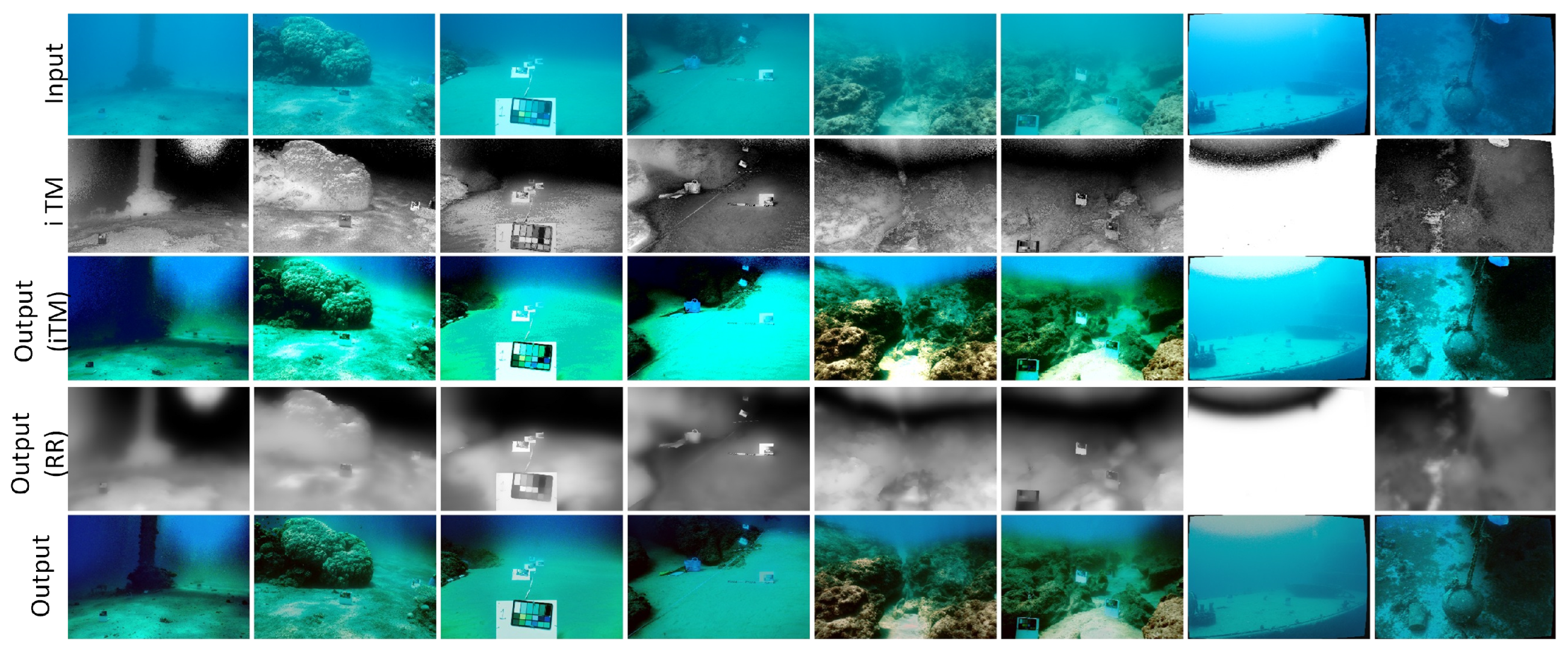
First, we selected 8 stereo pairs from the four benchmark datasets. Then two stereo pairs are chosen from each dataset, namely Katzaa, Michmoret, Nachsholis, and Satil, respectively, which can be seen in the first row of Figure 4. Afterward, the initial transmission maps are computed for each image (second row), where black and white colors represent the variation in transmission values. It is apparent that the edges of the objects are fused with the background, and the variation in the closed-depth regions is not smooth. If the images are recovered based on the wrong initial transmission maps, i.e., by replacing the $\widehat{t}\left(\mathbf{x}\right)=t\left(\mathbf{x}\right)$ in the (Equation (19)), the resulting images will be of poor quality (third row). Therefore, we come up with a robust non-convex regularizer in order to improve the initial transmission maps (fourth row). The output of the robust regulator (RR) is much better than the initial transmission maps, where the objects are not blended with the background. Also, the edges of the objects are much smoother, which shows a consistent result when it comes to the structure in the spatial domain. Finally, the input images are recovered using the (Equation (19)) and the refined transmission map $\widehat{t}\left(\mathbf{x}\right)$. The resultant restored images (last row) are more natural in terms of visibility compared to the output of initial transmission maps. The details of the images are well preserved with no blocking artifacts, which shows that the proposed method is helpful in improving the initial transmission maps.

Figure 4. The proposed robust method improves the initial transmission maps, leading to a visual improvement in the quality of the recovered images compared to the images recovered by initial transmission maps. The specific image details and corresponding quantitative measures $\rho$ and $\psi$ for each image can be found in Table 1.

Table 1 shows the quantitative analysis of the transmission maps and their outputs using the images from Figure 4. In this case, we used one measure, i.e., the Pearson correlation coefficient $\rho$, for the evaluation of transmission maps (Equation (21)), and one measure, i.e., average angular psi $\psi$, for the evaluation of restored colors (Equation (22)). For the first measure, the range of desired values is between −1 and 1, where values closer to 1 indicate a better estimation of the transmission maps, while values closer to 0 indicate a poorer estimation. For the second measure, the lower angle values represent a perfect color restoration. It is important to note that the $\psi$ values are computed on the neutral patches without using any global contrast adjustment. It is apparent that the computed values for $\rho$ on the refined transmission maps consistently increased (third col.) for each input image. Similarly, the results for the average angular error $\psi$ on the output images restored using the refined transmission maps give a lower error (fifth col.) compared to that of the initial $\psi$ values (fourth col.). This clearly indicates that refining the initial transmission maps using the proposed robust regularizer results in better restoration of quality images.

Table 1. Quantitative measures $\rho$ and $\psi$ computed for the images shown in Figure 4.

Images	Initial $\mathit{\rho }$	Refined $\mathit{\rho }$	Initial $\mathit{\psi }$	Refined $\mathit{\psi }$
RGT_4468	0.6398	0.7737	37.46	24.17
RGT_4493	0.6129	0.7425	37.08	30.81
RGT_5446	0.7469	0.8503	30.39	27.97
RGT_5480	0.2975	0.3353	35.25	31.56
RGT_2998	0.8457	0.8935	35.48	31.6
RGT_3276	0.8475	0.9141	41.93	31.73
RGT_4336	0.2597	0.302	35.45	31.88
RGT_4381	0.5166	0.5777	35.62	30.03

Now, we will look into the performance of the proposed regularization method presented in Figure 5. In this case, we computed initial transmission maps using the underwater haze line prior (UHLP) [3] by selecting one image from each dataset (Input). Next, initial transmission maps are refined using various state-of-the-art transmission refinement methods, namely guided filter [31], mutual structure filtering [32], soft matting [26], and SD filtering [25], respectively, along with our method RR (last column). It is clear that all methods are adequate for improving the initial transmission maps, and each of them (from GF to SDF) has issues like quick variations in the nearby depth regions, and the object edges are fused with the background.

Figure 5. An in-depth analysis of the proposed regularization method for underwater image enhancement. Initial transmission maps are computed using the underwater haze line prior and refined using various state-of-the-art methods, including GF (guided filter), MSF (mutual structure filtering), SM (soft matting), and SDF (SD filtering), with our method showing promising results in improving overall image quality despite some limitations in depth region and object edge distinction.

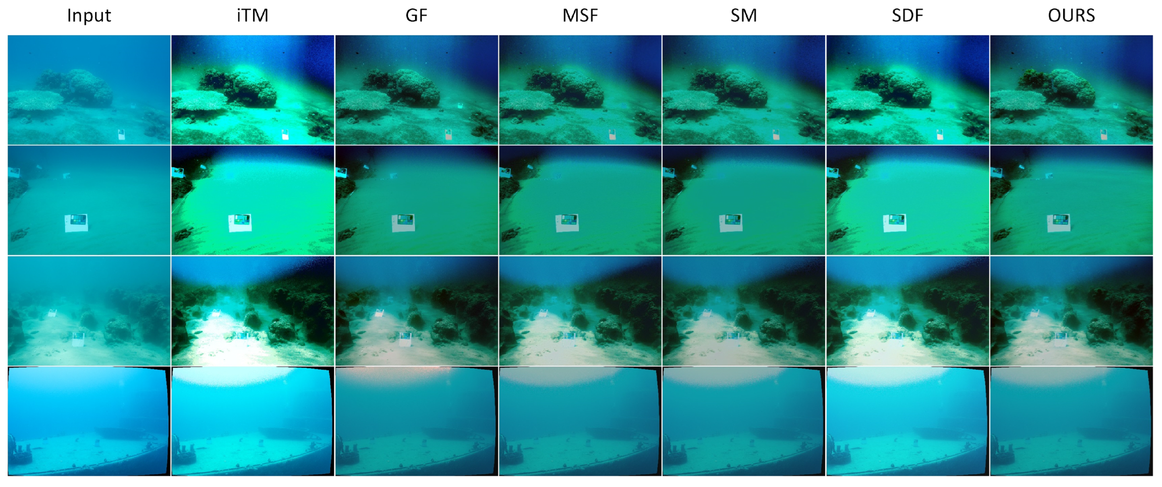
We also computed output for each refinement method Figure 6 to see the visibility of objects. Despite some limitations, all methods are sufficient for improving the initial transmission maps. However, the color variations in the edges from the foreground to the background are abrupt from guided filter to SD filtering. Mutual structure filtering and SDF both increased visibility, but the objects have become over-saturated. Also, the visibility of soft matting is poor, and object texture details are lost. On the other hand, it is interesting to note that GF surpassed the other methods, but our methodology, which provides natural results that are free from the above-mentioned artifacts, outperformed GF and other state-of-the-art improvement methods significantly.

Figure 6. A comparison of output for various refinement methods highlights the effectiveness of each in improving the visibility of objects in underwater images. While all methods show promise, there are limitations such as abrupt color variations and over-saturation. Our proposed methodology stands out as the best option, providing natural results without the artifacts present in other state-of-the-art improvement methods.

Table 2 and Table 3 present the results of our quantitative analysis on various transmission refinement methods, which includes the initial transmission values and their corresponding color evaluation using the unique measures $\rho$ (Equation (21)) and $\psi$ (Equation (22)). In Table 2, we compare the initial transmission values against the refinement methods guided filter, mutual structure filtering, SM, and SDF. Meanwhile, Table 3 presents the comparison of the restored images from the initial transmission map and refined map using the aforementioned methods, with the images from the Katzaa, Michmoret, Nachsholism, and Satil databases. Overall, these results suggest that our proposed method is a promising transmission refinement approach, and its effectiveness for color correction may depend on the characteristics of the input data.

Table 2. Quantitative measure of Pearson correlation coefficient $\rho$ for four datasets against various refinement methods.

Methods	Katzaa	Michmoret	Nachsholim	Satil
ITM	0.62	0.66	0.82	0.31
GF	0.66	0.72	0.85	0.33
MSF	0.64	0.68	0.84	0.34
SM	0.63	0.68	0.83	0.33
SDF	0.63	0.67	0.83	0.33
Our	0.7	0.73	0.87	0.37

Table 3. Quantitative measure of average angular error $\psi$ for four datasets against various refinement methods.

Methods	Katzaa	Michmoret	Nachsholim	Satil
ITM	35.39	33.58	35.51	36.59
GF	29.72	30.28	30	31.16
MSF	29.88	29.56	30.35	30.31
SM	30.28	30.16	30.51	31.15
SDF	32.33	29.51	31.09	30.25
Our	29.41	29.82	30.42	30.69

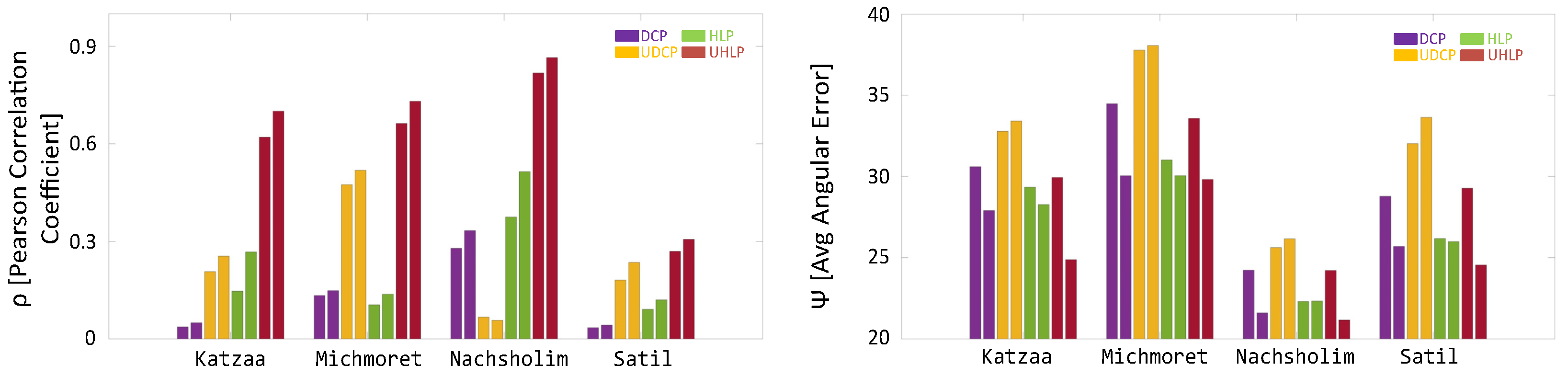
In another simulation, we conducted a quantitative analysis to assess the performance of our proposed regularization method when applied to various state-of-the-art methods. Figure 7 presents the quantitative analysis of the images from four different datasets. The $\rho$ and $\psi$ values were calculated for each method by replacing their refinement techniques with our robust regularization method. In this analysis, we evaluated several well-known methods for calculating initial transmission matrices: DCP, UDCP, HLP, and UHLP. The graph on the left side shows the improvement in initial transmission matrices, as measured by the Pearson correlation coefficient $\rho$. The first bar in each method represents the initial $\rho$ values, and the subsequent bar of the same color indicates the improvement in $\rho$ values after using our method. It can be observed that our method was effective at improving the initial transmission matrices in all of the selected methods. Similarly, the graph on the right side demonstrates the improvement in color values, represented by $\psi$. The color coding is the same as in the first graph. From this graph, it is clear that our method is able to reduce the average angular error $\psi$ in all methods. In our experiments, we also observed that our method improved the transmission of UDCP for a variety of images. However, there are some cases where the method fails to meet the assumptions of the model or encounters a low signal, leading to failure.

Figure 7. A quantitative measure is presented using all images from four datasets (Katzaa, Michmoret, Nachsholism, and Satil) for our robust transmission refinement method applied to various state-of-the-art techniques by replacing their refinement techniques, including DCP [26], UDCP [19], HLP [30], and UHLP [3]. The left-hand side graph compares improvement in initial transmission maps using $\rho$, while the right-hand side graph shows the color comparisons $\psi$ of restored images. The second bar, which is the same color as the first one, illustrates the improvement results.

4.3. Comparison

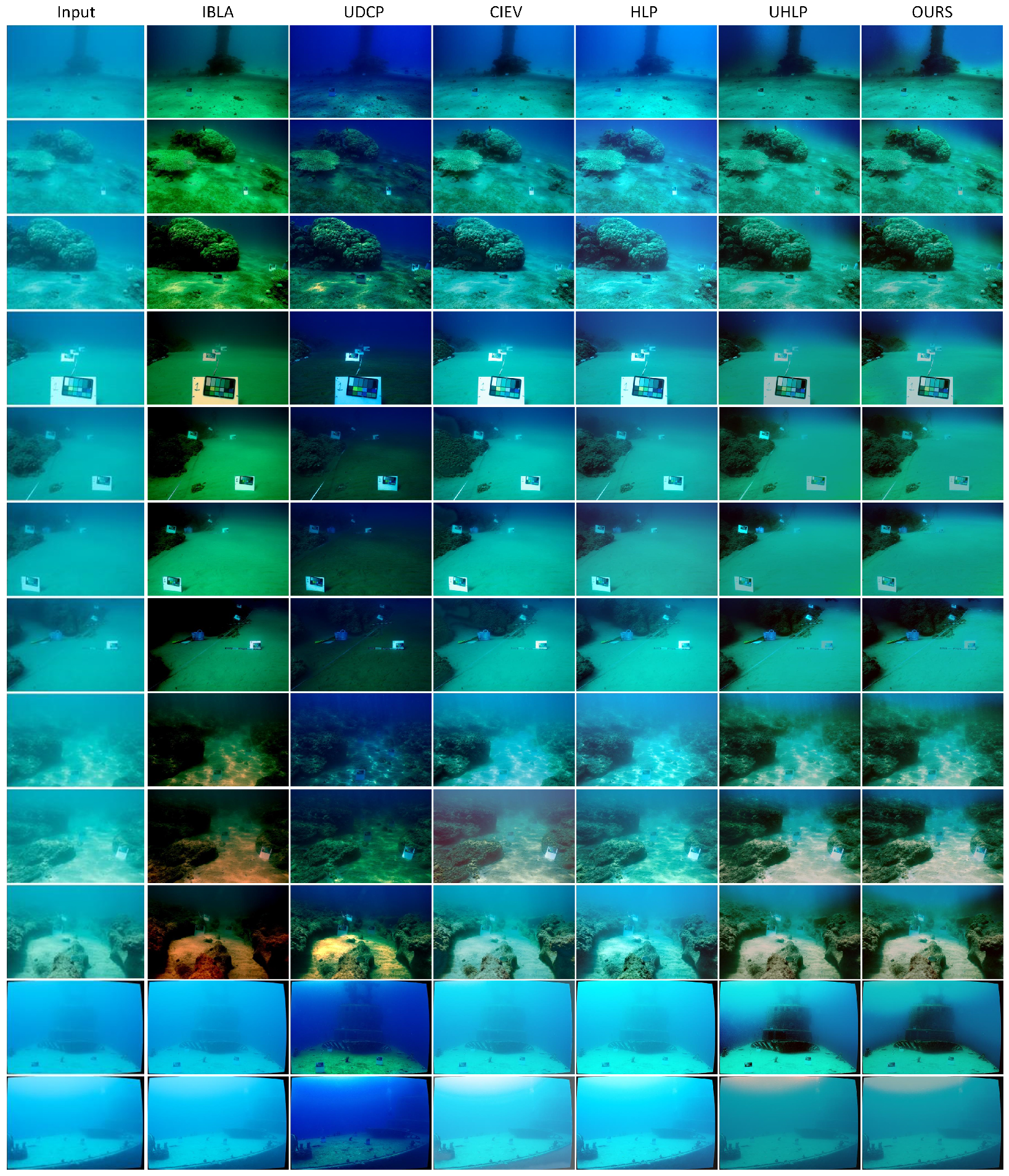
In this section, we evaluate the performance of the state-of-the-art (SOTA) and proposed methods through both qualitative and quantitative analyses. To compare the results of image restoration, we randomly select a subset of images from four datasets and present them in Figure 8. The first column shows the input images, and the remaining columns depict the output of each method, including our proposed method. The results for IBLA [27], UDCP [19], CEIV [40], HLP [30], and UHLP [3] were generated using code released by the respective authors.

Figure 8. This figure compares the performance of state-of-the-art and proposed methods for image restoration through a qualitative and quantitative analysis. The first column shows the input images, and the remaining columns depict the output of each method, including our proposed method. A qualitative comparison reveals that our proposed method not only effectively minimizes the haze but also restores the natural appearance of the scenes and preserves sharp structural edges and depth discontinuities. The results of IBLA [27], UDCP [19], CEIV [40], HLP [30], and UHLP [3] are also shown in the figure. The quantitative comparison in Table 4 using the images shown in Figure 8 shows that our proposed method outperforms various SOTA methods without using any contrast stretching. The specific image details and corresponding quantitative values for each image can be found in Table 4.

A qualitative comparison reveals that IBLA [27] effectively restores colors, even though with a slight tendency towards oversaturation across different distances. The method proposed by UDCP [19], which relies on the dark channel prior, was not able to consistently correct colors in the images. Similarly, the method proposed by CEIV [40] also failed to consistently correct colors and optimally preserve information in the images. The method proposed by HLP [30] was not effective in removing haze and contrast from the images, whereas the new method UHLP [3], proposed by the same author for handling different types of underwater images, is notably better at restoring colors. However, it should be noted that sharp structural edges are not well-preserved in this method. By examining the dehazed results in the last row, it can be observed that our proposed method not only effectively minimizes the haze but also restores the natural appearance of the scenes. Furthermore, the proposed regularizer with structural priors effectively preserves sharp structural edges and depth discontinuities.

In addition to the qualitative analysis, we also present a quantitative comparison in Table 4 using the images shown in Figure 8. The corresponding image number is mentioned in the first column. To facilitate the understanding of the evaluation results, we first compute the average angular error $\psi$, followed by the output of different underwater image enhancement methods. It should be noted that contrast stretching often outperforms most methods, especially on closer charts. We compared our method to others by using the same code and just changing the size of the images. However, in our case, we do not use any contrast stretching, and it is apparent that our proposed method outperforms various SOTA methods. 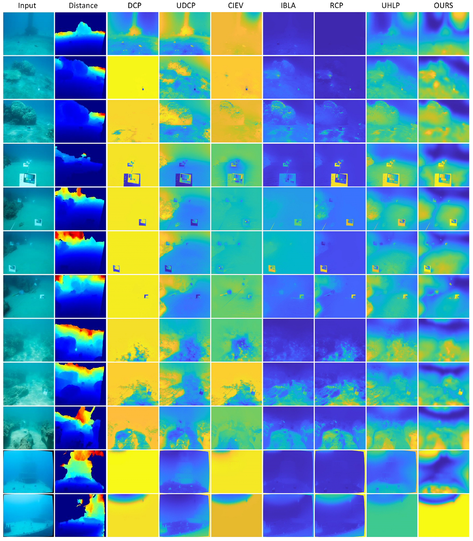Figure 9 illustrates the ground-truth distance and transmission maps for the images presented in Figure 8. The true distance is displayed in meters and is color-coded, with blue indicating missing distance values due to occlusions and unmatched pixels between the images. The selected images are from the right camera, which results in many missing distance values on the right border of the image, as these regions were not visible in the left camera.

Table 4. Comparisons of the average reproduction angular error $\psi$ in RGB space between the gray-scale patches and pure gray color for a few state-of-the-art methods, including the input. Lower values indicate better performance.

Images	Input $\mathit{\psi }$	IBLA [27]	UDCP [19]	CEIV [40]	HLP [30]	UHLP [3]	OURS
RGT_4479	35.883	36.679	47.316	36.817	37.363	32.107	29.835
RGT_4487	34.968	37.637	95.724	34.637	31.303	31.177	30.901
RGT_4493	35.472	44.468	78.108	35.687	30.196	30.815	30.813
RGT_5455	31.453	31.453	92.526	30.26	29.259	28.182	27.471
RGT_5466	34.845	36.788	87.083	34.525	30.736	31.727	30.956
RGT_5471	35.094	35.511	84.877	34.927	27.469	31.388	30.827
RGT_5480	34.613	37.333	85.437	33.979	33.027	31.718	31.561
RGT_2998	35.276	38.632	108.43	35.454	30.535	31.642	31.603
RGT_3014	34.403	36.351	111.23	16.372	29.891	30.2	30.403
RGT_3272	35.218	35.218	94.53	35.224	31.427	31.206	31.156

Figure 9. This figure compares the ground-truth distance and transmission maps for images shown in Figure 8. Our method effectively refines the transmission, taking into account the structures of the edges and depth to achieve a much smoother result. The quality of the transmission is quantitatively evaluated using the Pearson correlation coefficient $\rho$, which is calculated as the correlation between the negative logarithm of the estimated transmission and the true distance. This comparison provides insight into the accuracy of the transmission map estimates generated by each method. Our method outperforms state-of-the-art methods such as DCP [26], UDCP [19], CEIV [40], IBLA [27], RCP [21], and UHLP [3], as shown by the Pearson correlation coefficient in Table 4. The specific image details and corresponding quantitative values for each image can also be found in Table 4.

To compare the proposed method with state-of-the-art (SOTA) methods and showcase the diversity, a variety of methods were selected from Table 5, as well as other popular algorithms well-known for computing transmission maps, including DCP [26], UDCP [19], CEIV [40], IBLA [27], RCP [21], UHLP [3], and the proposed method. These transmission maps are estimated using a single image and are evaluated quantitatively based on the true distance map of each scene. The results indicate that the proposed method effectively refines the transmission by taking into account the structures of the edges and depth, resulting in a much smoother outcome. In contrast, methods such as UHLP that use the refinement method outlined in Figure 8 do not perform well in transferring structural information from guidance to transmission maps. Methods like DCP and RCP fail to refine the transmission, and the reasons for this failure are discussed in the quantitative evaluation below. Moreover, the proposed method is also robust to missing distance values issue, as it can handle occlusions and unmatched pixels between the images.

Table 5. The Pearson correlation coefficient $\rho$ between the estimated transmission maps and the ground truth distance for various images, as shown in Figure 8, are presented in each row of the figure. To ensure consistency, the distance is calculated in meters, and the correlation is determined between the distance and −log(t). Higher values indicate better performance.

Images	DCP [26]	UDCP [19]	CEIV [40]	IBLA [27]	RCP [21]	UHLP [3]	OURS
RGT_4479	0.084	−0.722	−0.379	0.86	0.392	0.816	0.878
RGT_4487	−0.026	−0.261	−0.018	0.677	0.158	0.779	0.843
RGT_4493	−0.116	−0.076	0.06	0.627	0.366	0.607	0.742
RGT_5455	−0.29	−0.504	−0.158	0.242	0.293	0.75	0.771
RGT_5466	−0.107	−0.326	−0.017	0.337	0.133	0.796	0.823
RGT_5471	−0.102	−0.695	−0.062	0.001	−0.05	0.799	0.776
RGT_5480	−0.031	−0.606	−0.001	−0.126	−0.28	0.31	0.335
RGT_2998	−0.275	0.0101	0.032	0.825	0.416	0.885	0.893
RGT_3014	−0.414	−0.057	−0.446	0.877	0.633	0.847	0.822
RGT_3272	−0.37	0.3716	−0.416	0.897	0.687	0.888	0.862
RGT_4318	0.057	0.0281	0.239	0.695	−0.04	0.353	0.361
RGT_4336	0.233	0.1742	0.267	0.473	−0.02	0.299	0.302

The quantitative comparison evaluated the performance of various methods for estimating transmission maps from a single image using the Pearson correlation coefficient $\rho$ as the evaluation metric. The results summarized in Table 5 indicate that the proposed method yields more accurate transmission maps compared to other methods. Some methods, such as UDCP [19] and CEIV [40], do not prioritize physically valid transmission maps, which may be due to their use of high values in the veiling light region to suppress noise. Most of the other methods show far-off transmission values, with the exception of IBLA [27], which performs slightly better on average but with the drawback of a highly color-biased scene correction. The proposed method outperforms the state-of-the-art methods without any contrast adjustments. Additionally, it is also worth noting that methods such as UDCP [19] and CEIV [40] may prioritize different aspects such as noise reduction, while the proposed method focuses on physically valid transmission maps.

4.4. Complexity Analysis

In order to estimate the time taken by different methods, we run DCP [26], UDCP [19], RCP [21] IBLA [27], HLP [30] and the proposed method on the system X64 bit-based PC having processor 11th generation Intel Core i9-11900K at our laboratory with 32 GB RAM for images having dimensions $256\times 256\times 3$ and calculated the processing time.

Table 6 shows the numerical values for time in seconds for various methods. RCP [21], DCP [26], and UDCP [19] methods are the most efficient, as the initial transmission is obtained using dark channel prior, and the refinement of the initial transmission map is carried out using guided filtering, so both operations are efficient. While techniques such as IBLA [27] and HLP [30] are computationally intensive for processing their initial transmission maps. In general, the proposed method can use the initial transmission map computed through any method. However, HLP [30] is chosen for its effectiveness in computing the initial transmission map, and then regularization is applied for its improvement. Although this makes the proposed method more computationally expensive than others, it achieves superior restoration quality.

Table 6. Time taken in (seconds) by different methods.

DCP [26]	UDCP [19]	RCP [21]	IBLA [27]	HLP [30]	Ours
0.68	0.69	0.05	5.21	4.06	5.66

5. Conclusions

This study presents a robust regularization technique for restoring high-quality underwater images by improving the initial transmission map. The proposed method addresses common challenges in underwater image restoration, such as artifacts and blurred boundaries, by introducing a nonconvex energy function for optimizing the initial transmission map. The method was found to be efficient and accurate when compared to various transmission refinement and enhancement methods using four benchmark datasets. The datasets contain different stereo pairs from the Red Sea and the Mediterranean Sea and were evaluated using realistic measures for transmission maps and color restoration. The regularization parameters used in the method were found to be critical and effective with the appropriate values mentioned in experimental setups. Empirical evaluations have shown the proposed method to significantly outperform existing state-of-the-art techniques in terms of refining the initial transmission maps and restoring high-quality underwater images.

Despite the improved performance and effectiveness of the proposed method, it presents notable limitations in terms of computational expense and the dependability on input. First, as the proposed method uses regularization, its optimization process needs extra computations. Therefore, the processing requirements are higher than comparable approaches. This limitation may impact its feasibility for large-scale or real-time applications, especially in resource-constrained environments. Secondly, note that the proposed method’s performance depends on the accuracy of the initial transmission map and may vary depending on the severity and types of the input images. Its performance may decrease in the presence of severe degradation, such as large amounts of back scattering and low light conditions. In these scenarios, initial transmission maps computed through various methods may suffer from inaccuracies and consequently leads for poor restorations.

Future work could explore optimizations or alternative algorithms to reduce these requirements while maintaining comparable performance. In addition, it would be interesting to explore the use of deep learning techniques in combination with the proposed regularization method to further improve the restoration of underwater images. Additionally, more extensive experiments on a wider range of underwater environments and image types would be beneficial in evaluating the methods and their generalization.

References

- Islam, M.J.; Xia, Y.; Sattar, J. Fast Underwater Image Enhancement for Improved Visual Perception. IEEE Robot. Autom. Lett. 2020, 5, 3227–3234. [Google Scholar] [CrossRef]
- Han, M.; Lyu, Z.; Qiu, T.; Xu, M. A Review on Intelligence Dehazing and Color Restoration for Underwater Images. IEEE Trans. Syst. Man Cybern. Syst. 2020, 50, 1820–1832. [Google Scholar] [CrossRef]
- Berman, D.; Levy, D.; Avidan, S.; Treibitz, T. Underwater Single Image Color Restoration Using Haze-Lines and a New Quantitative Dataset. IEEE Trans. Pattern Anal. Mach. Intell. 2021, 43, 2822–2837. [Google Scholar] [CrossRef]
- Treibitz, T.; Schechner, Y.Y. Active polarization descattering. IEEE Trans. Pattern Anal. Mach. Intell. 2008, 31, 385–399. [Google Scholar] [CrossRef]
- Murez, Z.; Treibitz, T.; Ramamoorthi, R.; Kriegman, D. Photometric stereo in a scattering medium. In Proceedings of the IEEE International Conference on Computer Vision, Santiago, Chile, 7–13 December 2015; pp. 3415–3423. [Google Scholar]
- Zhou, Y.; Wu, Q.; Yan, K.; Feng, L.; Xiang, W. Underwater image restoration using color-line model. IEEE Trans. Circuits Syst. Video Technol. 2018, 29, 907–911. [Google Scholar] [CrossRef]
- Guo, Y.; Li, H.; Zhuang, P. Underwater image enhancement using a multiscale dense generative adversarial network. IEEE J. Ocean. Eng. 2019, 45, 862–870. [Google Scholar] [CrossRef]
- Fu, X.; Cao, X. Underwater image enhancement with global–local networks and compressed-histogram equalization. Signal Process. Image Commun. 2020, 86, 115892. [Google Scholar] [CrossRef]
- Jian, M.; Liu, X.; Luo, H.; Lu, X.; Yu, H.; Dong, J. Underwater image processing and analysis: A review. Signal Process. Image Commun. 2021, 91, 116088. [Google Scholar] [CrossRef]
- Zhang, W.; Dong, L.; Zhang, T.; Xu, W. Enhancing underwater image via color correction and bi-interval contrast enhancement. Signal Process. Image Commun. 2021, 90, 116030. [Google Scholar] [CrossRef]
- Zhang, W.; Dong, L.; Xu, W. Retinex-inspired color correction and detail preserved fusion for underwater image enhancement. Comput. Electron. Agric. 2022, 192, 106585. [Google Scholar] [CrossRef]
- Liu, P.; Zhang, C.; Qi, H.; Wang, G.; Zheng, H. Multi-attention DenseNet: A scattering medium imaging optimization framework for visual data pre-processing of autonomous driving systems. IEEE Trans. Intell. Transp. Syst. 2022, 23, 25396–25407. [Google Scholar] [CrossRef]
- Liang, Z.; Ding, X.; Wang, Y.; Yan, X.; Fu, X. GUDCP: Generalization of underwater dark channel prior for underwater image restoration. IEEE Trans. Circuits Syst. Video Technol. 2021, 32, 4879–4884. [Google Scholar] [CrossRef]
- Ye, X.; Li, Z.; Sun, B.; Wang, Z.; Xu, R.; Li, H.; Fan, X. Deep joint depth estimation and color correction from monocular underwater images based on unsupervised adaptation networks. IEEE Trans. Circuits Syst. Video Technol. 2020, 30, 3995–4008. [Google Scholar] [CrossRef]
- Schechner, Y.Y.; Averbuch, Y. Regularized Image Recovery in Scattering Media. IEEE Trans. Pattern Anal. Mach. Intell. 2007, 29, 1655–1660. [Google Scholar] [CrossRef]
- Li, M.; Liu, J.; Yang, W.; Sun, X.; Guo, Z. Structure-Revealing Low-Light Image Enhancement Via Robust Retinex Model. IEEE Trans. Image Process. 2018, 27, 2828–2841. [Google Scholar] [CrossRef]
- Ali, U.; Mahmood, M.T. Underwater image restoration through regularization of coherent structures. Front. Mar. Sci. 2022, 9, 1024339. [Google Scholar] [CrossRef]
- Schechner, Y.Y.; Karpel, N. Recovery of underwater visibility and structure by polarization analysis. IEEE J. Ocean. Eng. 2005, 30, 570–587. [Google Scholar] [CrossRef]
- Drews, P.; Nascimento, E.; Moraes, F.; Botelho, S.; Campos, M. Transmission estimation in underwater single images. In Proceedings of the IEEE International Conference on Computer Vision Workshops, Sydney, Australia, 2–8 December 2013; pp. 825–830. [Google Scholar]
- Li, C.Y.; Guo, J.C.; Cong, R.M.; Pang, Y.W.; Wang, B. Underwater Image Enhancement by Dehazing with Minimum Information Loss and Histogram Distribution Prior. IEEE Trans. Image Process. 2016, 25, 5664–5677. [Google Scholar] [CrossRef]
- Galdran, A.; Pardo, D.; Picón, A.; Alvarez-Gila, A. Automatic Red-Channel underwater image restoration. J. Vis. Commun. Image Represent. 2015, 26, 132–145. [Google Scholar] [CrossRef]
- Gao, Y.; Li, H.; Wen, S. Restoration and Enhancement of Underwater Images Based on Bright Channel Prior. Math. Probl. Eng. 2016, 2016, 3141478. [Google Scholar] [CrossRef]
- Wang, S.; Chi, C.; Wang, P.; Zhao, S.; Huang, H.; Liu, X.; Liu, J. Feature-Enhanced Beamforming for Underwater 3-D Acoustic Imaging. IEEE J. Ocean. Eng. 2022, 48, 401–415. [Google Scholar] [CrossRef]
- Kenneth, L. MM Optimization Algorithms; SIAM: Philadelphia, PA, USA, 2016; p. 233. [Google Scholar] [CrossRef]
- Ham, B.; Cho, M.; Ponce, J. Robust Image Filtering using Joint Static and Dynamic Guidance. In Proceedings of the IEEE Conference on Computer Vision and Pattern Recognition (CVPR), Boston, MA, USA, 7–12 June 2015; IEEE: Piscataway, NJ, USA, 2015. [Google Scholar]
- He, K.; Sun, J.; Tang, X. Single image haze removal using dark channel prior. IEEE Trans. Pattern Anal. Mach. Intell. 2011, 33, 2341–2353. [Google Scholar] [PubMed]
- Peng, Y.T.; Cosman, P.C. Underwater Image Restoration Based on Image Blurriness and Light Absorption. IEEE Trans. Image Process. 2017, 26, 1579–1594. [Google Scholar] [CrossRef] [PubMed]
- Wang, Y.; Liu, H.; Chau, L.P. Single Underwater Image Restoration Using Adaptive Attenuation-Curve Prior. IEEE Trans. Circuits Syst. I Regul. Pap. 2018, 65, 992–1002. [Google Scholar] [CrossRef]
- Peng, Y.T.; Cao, K.; Cosman, P.C. Generalization of the Dark Channel Prior for Single Image Restoration. IEEE Trans. Image Process. 2018, 27, 2856–2868. [Google Scholar] [CrossRef]
- Berman, D.; Treibitz, T.; Avidan, S. Single image dehazing using haze-lines. IEEE Trans. Pattern Anal. Mach. Intell. 2018, 42, 720–734. [Google Scholar] [CrossRef] [PubMed]
- He, K.; Sun, J.; Tang, X. Guided Image Filtering. IEEE Trans. Pattern Anal. Mach. Intell. 2013, 35, 1397–1409. [Google Scholar] [CrossRef]
- Shen, X.; Zhou, C.; Xu, L.; Jia, J. Mutual-Structure for Joint Filtering. In Proceedings of the IEEE International Conference on Computer Vision (ICCV), Santiago, Chile, 7–15 December 2015. [Google Scholar]
- Liu, R.; Ma, L.; Zhang, J.; Fan, X.; Luo, Z. Retinex-inspired unrolling with cooperative prior architecture search for low-light image enhancement. In Proceedings of the IEEE/CVF Conference on Computer Vision and Pattern Recognition, Nashville, TN, USA, 20–25 June 2021; pp. 10561–10570. [Google Scholar]
- Dong, L.; Zhang, W.; Xu, W. Underwater image enhancement via integrated RGB and LAB color models. Signal Process. Image Commun. 2022, 104, 116684. [Google Scholar] [CrossRef]
- Ancuti, C.; Ancuti, C.O.; Haber, T.; Bekaert, P. Enhancing underwater images and videos by fusion. In Proceedings of the 2012 IEEE Conference on Computer Vision and Pattern Recognition, Providence, RI, USA, 16–21 June 2012; pp. 81–88. [Google Scholar] [CrossRef]
- Ancuti, C.O.; Ancuti, C.; De Vleeschouwer, C.; Bekaert, P. Color Balance and Fusion for Underwater Image Enhancement. IEEE Trans. Image Process. 2018, 27, 379–393. [Google Scholar] [CrossRef]
- Tan, C.; Seet, G.; Sluzek, A.; He, D. A novel application of range-gated underwater laser imaging system (ULIS) in near-target turbid medium. Opt. Lasers Eng. 2005, 43, 995–1009. [Google Scholar] [CrossRef]
- Zhao, Y.; He, W.; Ren, H.; Li, Y.; Fu, Y. Polarization descattering imaging through turbid water without prior knowledge. Opt. Lasers Eng. 2022, 148, 106777. [Google Scholar] [CrossRef]
- Li, J.; Li, Y. Underwater image restoration algorithm for free-ascending deep-sea tripods. Opt. Laser Technol. 2019, 110, 129–134. [Google Scholar] [CrossRef]
- Kim, J.H.; Jang, W.D.; Sim, J.Y.; Kim, C.S. Optimized contrast enhancement for real-time image and video dehazing. J. Vis. Commun. Image Represent. 2013, 24, 410–425. [Google Scholar] [CrossRef]
- Zhang, W.; Zhuang, P.; Sun, H.H.; Li, G.; Kwong, S.; Li, C. Underwater Image Enhancement via Minimal Color Loss and Locally Adaptive Contrast Enhancement. IEEE Trans. Image Process. 2022, 31, 3997–4010. [Google Scholar] [CrossRef] [PubMed]
- Xie, J.; Hou, G.; Wang, G.; Pan, Z. A variational framework for underwater image dehazing and deblurring. IEEE Trans. Circuits Syst. Video Technol. 2021, 32, 3514–3526. [Google Scholar] [CrossRef]
- Wang, Y.; Zhang, J.; Cao, Y.; Wang, Z. A deep CNN method for underwater image enhancement. In Proceedings of the 2017 IEEE International Conference on Image Processing (ICIP), Beijing, China, 17–20 September 2017; pp. 1382–1386. [Google Scholar] [CrossRef]
- Li, C.; Anwar, S.; Porikli, F. Underwater scene prior inspired deep underwater image and video enhancement. Pattern Recognit. 2020, 98, 107038. [Google Scholar] [CrossRef]
- Yang, M.; Hu, K.; Du, Y.; Wei, Z.; Sheng, Z.; Hu, J. Underwater image enhancement based on conditional generative adversarial network. Signal Process. Image Commun. 2020, 81, 115723. [Google Scholar] [CrossRef]
- Song, Y.; He, Z.; Qian, H.; Du, X. Vision transformers for single image dehazing. IEEE Trans. Image Process. 2023, 32, 1927–1941. [Google Scholar] [CrossRef]
- Wang, Z.; Zhang, K.; Yang, Z.; Da, Z.; Huang, S.; Wang, P. Underwater Image Enhancement Based on Improved U-Net Convolutional Neural Network. In Proceedings of the 2023 IEEE 18th Conference on Industrial Electronics and Applications (ICIEA), Ningbo, China, 18–22 August 2023; IEEE: Piscataway, NJ, USA, 2023; pp. 1902–1908. [Google Scholar]
- Deng, X.; Liu, T.; He, S.; Xiao, X.; Li, P.; Gu, Y. An underwater image enhancement model for domain adaptation. Front. Mar. Sci. 2023, 10, 1138013. [Google Scholar] [CrossRef]
- Liao, K.; Peng, X. Underwater image enhancement using multi-task fusion. PLoS ONE 2024, 19, e0299110. [Google Scholar] [CrossRef]
- Krishnan, D.; Fattal, R.; Szeliski, R. Efficient preconditioning of laplacian matrices for computer graphics. ACM Trans. Graph. (tOG) 2013, 32, 1–15. [Google Scholar] [CrossRef]
- SQUID- Stereo Quantitative Underwater Image Dataset. Available online: https://csms.haifa.ac.il/profiles/tTreibitz/datasets/ambient_forwardlooking/ (accessed on 1 September 2024).
- Venkatanath, N.; Praneeth, D.; Bh, M.C.; Channappayya, S.S.; Medasani, S.S. Blind image quality evaluation using perception based features. In Proceedings of the 2015 Twenty First National Conference on Communications (NCC), Mumbai, India, 27 February–1 March 2015; pp. 1–6. [Google Scholar] [CrossRef]
- Mittal, A.; Soundararajan, R.; Bovik, A.C. Making a “Completely Blind” Image Quality Analyzer. IEEE Signal Process. Lett. 2013, 20, 209–212. [Google Scholar] [CrossRef]
- Mittal, A.; Moorthy, A.K.; Bovik, A.C. No-Reference Image Quality Assessment in the Spatial Domain. IEEE Trans. Image Process. 2012, 21, 4695–4708. [Google Scholar] [CrossRef] [PubMed]
- Li, C.; Guo, J.; Guo, C. Emerging From Water: Underwater Image Color Correction Based on Weakly Supervised Color Transfer. IEEE Signal Process. Lett. 2018, 25, 323–327. [Google Scholar] [CrossRef]
- Finlayson, G.D.; Zakizadeh, R. Reproduction angular error: An improved performance metric for illuminant estimation. Perception 2014, 310, 1–26. [Google Scholar]
Disclaimer/Publisher’s Note: The statements, opinions and data contained in all publications are solely those of the individual author(s) and contributor(s) and not of MDPI and/or the editor(s). MDPI and/or the editor(s) disclaim responsibility for any injury to people or property resulting from any ideas, methods, instructions or products referred to in the content. |
© 2024 by the authors. Licensee MDPI, Basel, Switzerland. This article is an open access article distributed under the terms and conditions of the Creative Commons Attribution (CC BY) license (https://creativecommons.org/licenses/by/4.0/).