Wave Speeds for a Time-Periodic Bistable Three-Species Lattice Competition System

Abstract

In this paper, we consider propagation direction (which can be used to predict which species will occupy the habitat or win the competition eventually) of a bistable wave for a three-species time-periodic lattice competition system with bistable nonlinearity, aiming to address an open problem. As a first step, by transforming the competition system to a cooperative one, we study the asymptotic behavior for the bistable wave profile and then prove the uniqueness of the bistable wave speed. Secondly, we utilize comparison principle and build up two couples of upper and lower solutions to judge the sign of the bistable wave speed which partially provides the answer to the open problem. As an application, we reduce the time-periodic system to a space–time homogeneous system, we obtain the corresponding criteria and carry out numerical simulations to illustrate the availability of our results. Moreover, an interesting phenomenon we have found is that the two weak competitors can wipe out the strong competitor under some circumstances.

1. Introduction

This paper is devoted to the propagation direction, which is determined by the sign of wave speed, of traveling wave solutions (TWSs) for the following bistable lattice system

$$\left\{\begin{array}{cc}\hfill u_j^{\prime }\left(t\right)& =d_1\left(t\right){\mathcal{D}}_2\left[u_j\right]\left(t\right)+u_j\left(t\right)(r_1\left(t\right)-a_{11}\left(t\right)u_j\left(t\right)-a_{12}\left(t\right)v_j\left(t\right)),\hfill \\ \hfill v_j^{\prime }\left(t\right)& =d_2\left(t\right){\mathcal{D}}_2\left[v_j\right]\left(t\right)+v_j\left(t\right)(r_2\left(t\right)-b_{11}\left(t\right)v_j\left(t\right)-b_{12}\left(t\right)u_j\left(t\right)-b_{13}\left(t\right)w_j\left(t\right)),\hfill \\ \hfill w_j^{\prime }\left(t\right)& =d_3\left(t\right){\mathcal{D}}_2\left[w_j\right]\left(t\right)+w_j\left(t\right)(r_3\left(t\right)-c_{11}\left(t\right)w_j\left(t\right)-c_{12}\left(t\right)v_j\left(t\right)),j\in \mathbb{Z},t>0.\hfill \end{array}\right.$$

(1)

In model (1) and in the sense of biology, one can interpret $u_j\left(t\right),v_j\left(t\right)$ and $w_j\left(t\right)$ as the population densities of three species at position j and time t, respectively, $d_i\left(t\right)$ as the diffusivity coefficient and $r_i\left(t\right)$ as the growth rate of the species. Here, the coefficients $a_{1i}\left(t\right),c_{1i}\left(t\right),i=1,2$ and $d_k\left(t\right),b_{1k}\left(t\right),k=1,2,3$ are assumed to be positive T-periodic functions with T being a positive number. Biologically speaking, $a_{1i}\left(t\right),b_{1k}\left(t\right),c_{1i}\left(t\right)$ are the intra-specific competitive coefficients as $i=k=1$, while $i=2$ or $k=2,3$, they represent the inter-specific competitive coefficients. The term ${\mathcal{D}}_2\left[s_j\right]\left(t\right)$ appearing in (1) is the second-order central difference and is defined as ${\mathcal{D}}_2\left[s_j\right]\left(t\right):=s(t,j+1)+s(t,j-1)-2s(t,j)$ for $s=u,v,w$. Evidently, system (1) is a competitive system and models such a relationship between three species: v competes with u and w for common resources, while there is no competition between u and w. The biological interpretation is that species u and w have different preferences for food resources, while species v has the same food preferences as u and w.

As we all know, nature is a constantly changing and relatively stable system, in which competition for survival between species is a common phenomenon. Therefore, to study the dynamic behavior between different species, it is necessary to study the phenomenon of competition between species and establish a reasonable model. The Lotka–Volterra competitive diffusion system is one of the classical biological models to describe inter- and intra-specific interactions. When the environment is assumed to be homogenous, the general form of the three-species Lotka–Volterra competition diffusion model in the above biological context is as follows:

$$\left\{\begin{array}{cc}& u_t=d_1{u}_{xx}+r_{1}u(1-u-a_{1}v),\hfill \\ & v_t=d_2{v}_{xx}+r_{2}v(1-v-a_{2}u-a_{3}w),\hfill \\ & w_t=d_3{w}_{xx}+r_{3}w(1-w-a_{4}v),t\in {\mathbb{R}}^{+},x\in \mathbb{R},\hfill \end{array}\right.$$

(2)

where $d_k,r_k,k=1,2,3$ and $a_l,l=1,2,3,4$ are positive constants. As a matter of fact, system (2) can be regarded as an extension of the classic two-species Lotka–Volterra system which has been studied extensively in past decades; see, for example, [1,2,3,4,5,6,7] and references therein. Due to the benefit from the classic Lotka–Volterra system in the application of ecology, more and more works have also been devoted to system (2). For instance, we refer the readers to [8,9] for the selection mechanism of minimum wave speed in the monostable model; [10] for the stability of monotone traveling wave solutions; ref. [11] for the exact traveling wave solutions of (2) with nontrivial three components; ref. [12] for the uniqueness of traveling wavefronts; and ref. [13,14] for the sign of wave speed in the bistable model. Related to the present paper, we particularly mention that Guo et al. [13] studied two different cases for system (2): (1) the case where two species are weakly competitive and one species is strongly competitive, and (2) the case where all three species are very strong competitors. They obtained some new observations in contrast with the two-species Lotka–Volterra model. In addition to system (2), we further refer the readers to [15,16,17,18,19] for a discrete three-species competition system; refs. [20,21] for a three-component competition system with nonlocal dispersal; and refs. [22,23] for a competitive–cooperative Lotka–Volterra system of three species.

In their recent paper, besides model (2), Guo et al. [13] also proposed a discrete version of (2), as follows:

$$\left\{\begin{array}{cc}& u_j^{\prime }\left(t\right)=d_1{\mathcal{D}}_2\left[u_j\right]\left(t\right)+r_1\left[u_j(1-u_j-b_2{v}_j)\right]\left(t\right),\hfill \\ & v_j^{\prime }\left(t\right)=d_2{\mathcal{D}}_2\left[v_j\right]\left(t\right)+r_2\left[v_j(1-b_1{u}_j-v_j-b_3{w}_j)\right]\left(t\right),\hfill \\ & w_j^{\prime }\left(t\right)=d_3{\mathcal{D}}_2\left[w_j\right]\left(t\right)+r_3\left[w_j(1-b_2{v}_j-w_j)\right]\left(t\right),t\in {\mathbb{R}}^{+},j\in \mathbb{Z},\hfill \end{array}\right.$$

(3)

where the parameters $d_k,r_k$ and $b_k,k=1,2,3$ are positive numbers and can be interpreted as the ones in system (2). In (3), although the sign of wave speed of (2) has been addressed for certain special cases, it is still largely left open for the discrete case (3). One of the reasons is that their method used on system (2) relies on the integration of the corresponding wave profile system, so it seems that such a method cannot be applied to system (3) directly due to the central difference involved in (3). Another reason might be that the combination of patchy environments and periodicity can make the corresponding analysis more difficult. In this paper, we try to make some progress in this direction and this is our main motivation. Our strategy is to use the upper/lower solution method to investigate the sign of the bistable wave speed of (1). As a matter of fact, this method has been proved to be valid in this subject for several diffusion systems; see, for instance, [4,6,9,24].

In recent years, an increasing number of scholars are attracted to traveling wave solutions that have advantages in describing the development, migration and invasion of biological populations. In particular, the sign of wave speed of traveling wave solutions can be used to explain the outcome of competition between different species, which makes it a meaningful topic. In this paper, we will study the propagation direction of traveling wave solutions for (1) which is a lattice competition system. To the best of our knowledge, the research of lattice dynamical systems, which are more in line with nature, originated from Bunimovich and Sinai [25] in 1988. After that, lattice dynamical models have widely been used in biological issues; see, for example, [6,26,27,28,29,30]. Generally speaking, these models are more effective in the case of species living in patchy environments.

Evidently, the corresponding space-homogenous ordinary differential system of (1) is as follows:

$$\left\{\begin{array}{cc}\hfill u^{\prime }\left(t\right)& =u\left(t\right)[r_1\left(t\right)-a_{11}\left(t\right)u\left(t\right)-a_{12}\left(t\right)v\left(t\right)],\hfill \\ \hfill v^{\prime }\left(t\right)& =v\left(t\right)[r_2\left(t\right)-b_{11}\left(t\right)v\left(t\right)-b_{12}\left(t\right)u\left(t\right)-b_{13}\left(t\right)w\left(t\right)],\hfill \\ \hfill w^{\prime }\left(t\right)& =w\left(t\right)[r_3\left(t\right)-c_{11}\left(t\right)w\left(t\right)-c_{12}\left(t\right)v\left(t\right)],t\in {\mathbb{R}}^{+}.\hfill \end{array}\right.$$

(4)

It is easy to see that system (4) at least has three nonnegative T-periodic solutions, which are the equilibrium points of (1). We denote them by $e_0:=(0,0,0), e_1:=(0,q\left(t\right),0),$ $e_2:=(p\left(t\right),0,r\left(t\right))$, respectively, in which $p\left(t\right),q\left(t\right),r\left(t\right)$ can be expressed as

$$p\left(t\right)={\displaystyle \frac{p_0{e}^{{\int }_0^t{r}_1\left(s\right)ds}}{p_0{\int }_0^t{a}_{11}\left(s\right)e^{{\int }_0^s{r}_1\left(\theta \right)d\theta }ds+1}},p_0={\displaystyle \frac{e^{{\int }_0^T{r}_1\left(s\right)ds}-1}{{\int }_0^T{a}_{11}\left(s\right)e^{{\int }_0^s{r}_1\left(\theta \right)d\theta }ds}},$$

$$q\left(t\right)={\displaystyle \frac{q_0{e}^{{\int }_0^t{r}_2\left(s\right)ds}}{q_0{\int }_0^t{b}_{11}\left(s\right)e^{{\int }_0^s{r}_2\left(\theta \right)d\theta }ds+1}},q_0={\displaystyle \frac{e^{{\int }_0^T{r}_2\left(s\right)ds}-1}{{\int }_0^T{b}_{11}\left(s\right)e^{{\int }_0^s{r}_2\left(\theta \right)d\theta }ds}},$$

$$r\left(t\right)={\displaystyle \frac{r_0{e}^{{\int }_0^t{r}_3\left(s\right)ds}}{r_0{\int }_0^t{c}_{11}\left(s\right)e^{{\int }_0^s{r}_3\left(\theta \right)d\theta }ds+1}},r_0={\displaystyle \frac{e^{{\int }_0^T{r}_3\left(s\right)ds}-1}{{\int }_0^T{c}_{11}\left(s\right)e^{{\int }_0^s{r}_3\left(\theta \right)d\theta }ds}}.$$

It is straightforward to check that $p\left(t\right), q\left(t\right)$ and $r\left(t\right)$ are T-periodic functions and satisfy $p(t+T)=p\left(t\right),q(t+T)=q\left(t\right)$ and $r(t+T)=r\left(t\right)$ for all $t\in {\mathbb{R}}^{+}$.

Since our main focus is on bistable waves of (1), we have to make the following assumption throughout this paper:

(A)

${\int }_0^T{r}_1\left(t\right)dt<{\int }_0^T{a}_{12}\left(t\right)q\left(t\right)dt$, ${\int }_0^T{r}_2\left(t\right)dt<{\int }_0^T{b}_{12}\left(t\right)p\left(t\right)+b_{13}\left(t\right)r\left(t\right)dt$ and ${\int }_0^T{r}_3\left(t\right)dt<{\int }_0^T{c}_{12}\left(t\right)q\left(t\right)dt$,

so that $e_1$ and $e_2$ are linearly stable equilibrium points.

As mentioned above, we are concerned with the periodic traveling wave of system (1), which bears the form of

$$\left(\begin{array}{c}{u}_j\left(t\right)\\ v_j\left(t\right)\\ w_j\left(t\right)\end{array}\right)=\left(\begin{array}{c}U(t,j+ct)\\ V(t,j+ct)\\ W(t,j+ct)\end{array}\right)=:\left(\begin{array}{c}U(t,z)\\ V(t,z)\\ W(t,z)\end{array}\right),z=j+ct,$$

(5)

satisfying

$$\left(\begin{array}{c}U(t+T,z)\\ V(t+T,z)\\ W(t+T,z)\end{array}\right)=\left(\begin{array}{c}U(t,z)\\ V(t,z)\\ W(t,z)\end{array}\right),$$

and is subject to the boundary conditions

$$(U,V,W)(t,-\infty )=(0,0,0),(U,V,W)(t,+\infty )=(1,1,1),$$

(6)

where c is the wave speed. The limits in (6) hold uniformly in $t\in {\mathbb{R}}^{+}$.

After a substitution of (5), (1) can be rewritten as a wave profile system

$$\left\{\begin{array}{cc}\hfill U_t+c{U}_z& =d_1\left(t\right){\mathcal{D}}_2\left[U\right](t,z)+U(r_1\left(t\right)-a_{11}\left(t\right)U-a_{12}\left(t\right)V),\hfill \\ \hfill V_t+c{V}_z& =d_2\left(t\right){\mathcal{D}}_2\left[V\right](t,z)+V(r_2\left(t\right)-b_{11}\left(t\right)V-b_{12}\left(t\right)U-b_{13}\left(t\right)W),\hfill \\ \hfill W_t+c{W}_z& =d_3\left(t\right){\mathcal{D}}_2\left[W\right](t,z)+W(r_3\left(t\right)-c_{11}\left(t\right)W-c_{12}\left(t\right)V),\hfill \end{array}\right.$$

(7)

where ${\mathcal{D}}_2\left[S\right](t,z)=S(t,z+1)+S(t,z-1)-2S(t,z)$ for $S=U,V,W$. Via the following changes

$$\Phi (t,z)={\displaystyle \frac{p\left(t\right)-U(t,z)}{p\left(t\right)}},\Psi (t,z)={\displaystyle \frac{V(t,z)}{q\left(t\right)}},\Theta (t,z)={\displaystyle \frac{r\left(t\right)-W(t,z)}{r\left(t\right)}},$$

system (7) can be converted into a cooperative system

$$\left\{\begin{array}{cc}& d_1\left(t\right){\mathcal{D}}_2[\Phi ](t,z)-c{\Phi }_z+(1-\Phi )[a_{12}\left(t\right)q\left(t\right)\Psi -a_{11}\left(t\right)p\left(t\right)\Phi ]={\Phi }_t,\hfill \\ & d_2\left(t\right){\mathcal{D}}_2[\Psi ](t,z)-c{\Psi }_z+\Psi [b_{11}\left(t\right)q\left(t\right)(1-\Psi )-b_{12}\left(t\right)p\left(t\right)(1-\Phi )-b_{13}\left(t\right)r\left(t\right)(1-\Theta )]={\Psi }_t,\hfill \\ & d_3\left(t\right){\mathcal{D}}_2[\Theta ](t,z)-c{\Theta }_z+(1-\Theta )[c_{12}\left(t\right)q\left(t\right)\Psi -c_{11}\left(t\right)r\left(t\right)\Theta ]={\Theta }_t,\hfill \end{array}\right.$$

(8)

with periodic conditions and boundary conditions (6) becoming

$$\left\{\begin{array}{cc}& (\Phi ,\Psi ,\Theta )(t,z)=(\Phi ,\Psi ,\Theta )(t+T,z),\hfill \\ & (\Phi ,\Psi ,\Theta )(t,-\infty )=(0,0,0),(\Phi ,\Psi ,\Theta )(t,+\infty )=(1,1,1).\hfill \end{array}\right.$$

For the sake of convenience, we shall call the first equation of (8) $\Phi$-equation, the second equation $\Psi$-equation and the last one $\Theta$-equation throughout this paper. Note that the existence of a bistable periodic traveling wave solution of (1) can be proved by following the ideas in [16,31], or by the abstract theory established in [32].

The remainder of this paper is organized as follows. In Section 2, we investigate the asymptotic behaviors of $\Phi (t,z),\Psi (t,z)$ and $\Theta (t,z)$ as the co-moving coordinate z tends to infinity, upon which the uniqueness of bistable wave speed is considered. In Section 3, we derive two crucial theorems concerning the determination of the sign of the bistable wave speed by employing the comparison principle. We construct suitable upper/lower solutions to obtain explicit conditions in Section 4, and the results of numerical simulation are shown in Section 5.

2. Uniqueness of Bistable Wave-Speed

To facilitate the forthcoming calculation and statement, we define some mathematical notations as follows:

$$\begin{array}{cc}\hfill & \overline{f\left(t\right)}:={\displaystyle \frac{1}{T}}{\int }_0^{T}f\left(t\right)dt,{\Delta }_1\left(t\right):=b_{11}\left(t\right)q\left(t\right)-b_{12}\left(t\right)p\left(t\right)-b_{13}\left(t\right)r\left(t\right),\hfill \\ \hfill & {\Delta }_2\left(t\right):=a_{11}\left(t\right)p\left(t\right)-a_{12}\left(t\right)q\left(t\right),{\Delta }_3\left(t\right):=c_{11}\left(t\right)r\left(t\right)-c_{12}\left(t\right)q\left(t\right),\hfill \\ \hfill & {\Gamma }_1(t,\mu ):=d_1\left(t\right)(e^{\mu }+e^{-\mu }-2)-c\mu -a_{11}\left(t\right)p\left(t\right),\hfill \\ \hfill & {\Gamma }_2(t,\mu ):=d_3\left(t\right)(e^{\mu }+e^{-\mu }-2)-c\mu -c_{11}\left(t\right)r\left(t\right),\hfill \\ \hfill & {\Gamma }_3(t,\mu ):=d_2\left(t\right)(e^{\mu }+e^{-\mu }-2)+c\mu -b_{11}\left(t\right)q\left(t\right).\hfill \end{array}$$

To investigate the asymptotic behavior of the bistable wave profile, we denote the unique positive solutions of the following equations

$$\begin{array}{cc}\hfill & \overline{d_2\left(t\right)}(e^{\mu }+e^{-\mu }-2)-c\mu +\overline{{\Delta }_1\left(t\right)}=0,\hfill \\ \hfill & \overline{d_1\left(t\right)}(e^{\mu }+e^{-\mu }-2)-c\mu -\overline{a_{11}\left(t\right)p\left(t\right)}=0,\hfill \\ \hfill & \overline{d_3\left(t\right)}(e^{\mu }+e^{-\mu }-2)-c\mu -\overline{c_{11}\left(t\right)r\left(t\right)}=0,\hfill \end{array}$$

by ${\mu }_1\left(c\right),{\mu }_2\left(c\right),{\mu }_3\left(c\right)$, respectively. Moreover, by a simple analysis, it is not hard to find that ${\mu }_1\left(c\right)$, ${\mu }_2\left(c\right)$ and ${\mu }_3\left(c\right)$ are increasing functions in c. Meanwhile, we denote ${\mu }_4\left(c\right)$, ${\mu }_5\left(c\right)$ and ${\mu }_6\left(c\right)$, respectively, by the unique positive roots of the following equations

$$\begin{array}{cc}\hfill & \overline{d_1\left(t\right)}(e^{\mu }+e^{-\mu }-2)+c\mu +\overline{{\Delta }_2\left(t\right)}=0,\hfill \\ \hfill & \overline{d_3\left(t\right)}(e^{\mu }+e^{-\mu }-2)+c\mu +\overline{{\Delta }_3\left(t\right)}=0,\hfill \\ \hfill & \overline{d_2\left(t\right)}(e^{\mu }+e^{-\mu }-2)+c\mu -\overline{b_{11}\left(t\right)q\left(t\right)}=0.\hfill \end{array}$$

Here, ${\mu }_4\left(c\right)$, ${\mu }_5\left(c\right)$, ${\mu }_6\left(c\right)$ are decreasing functions in c.

Based on the above notations, we are already to give the following lemma.

Lemma 1.

As $z\to -\infty$, the wave profile $(\Phi ,\Psi ,\Theta )(t,z)$ behaves like

$$\left(\begin{array}{c}\Phi (t,z)\\ \Psi (t,z)\\ \Theta (t,z)\end{array}\right)\sim A_1\left(\begin{array}{c}{\varphi }_{01}^{*}\left(t\right)\\ {\psi }_{01}\left(t\right)\\ {\theta }_{01}^{*}\left(t\right)\end{array}\right)e^{{\mu }_{1}z}+A_2\left(\begin{array}{c}{\varphi }_{01}\left(t\right)\\ 0\\ 0\end{array}\right)e^{{\mu }_{2}z}+A_3\left(\begin{array}{c}0\\ 0\\ {\theta }_{01}\left(t\right)\end{array}\right)e^{{\mu }_{3}z},$$

(9)

where ${\mu }_1\ne {\mu }_2\ne {\mu }_3$ and it holds uniformly in $t\in {\mathbb{R}}^{+}$. As $z\to \infty$, the wave profile $(\Phi ,\Psi ,\Theta )(t,z)$ behaves like

$$\left(\begin{array}{c}\Phi (t,z)\\ \Psi (t,z)\\ \Theta (t,z)\end{array}\right)\sim \left(\begin{array}{c}1\\ 1\\ 1\end{array}\right)-B_1\left(\begin{array}{c}{\varphi }_{11}\left(t\right)\\ {\psi }_{11}^{*}\left(t\right)\\ 0\end{array}\right)e^{-{\mu }_{4}z}-B_2\left(\begin{array}{c}0\\ {\psi }_{11}^{**}\left(t\right)\\ {\theta }_{11}\left(t\right)\end{array}\right)e^{-{\mu }_{5}z}-B_3\left(\begin{array}{c}0\\ {\psi }_{11}\left(t\right)\\ 0\end{array}\right)e^{-{\mu }_{6}z},$$

(10)

where ${\mu }_4\ne {\mu }_5\ne {\mu }_6$ and it holds uniformly in $t\in {\mathbb{R}}^{+}$. In the above formulas, $A_i,B_i,$$i=1,2,3$ are nonnegative numbers. The functions ${\psi }_{01}\left(t\right),{\varphi }_{01}\left(t\right),{\theta }_{01}\left(t\right),{\varphi }_{01}^{*}\left(t\right),$${\theta }_{01}^{*}\left(t\right)$ are defined as (14), (18), (19), (21) and (22), respectively; and ${\varphi }_{11}\left(t\right),{\theta }_{11}\left(t\right),{\psi }_{11}\left(t\right),{\psi }_{11}^{*}\left(t\right),$${\psi }_{11}^{**}\left(t\right)$ are defined as (25), (26), (29), (30) and (31), respectively.

Proof. 

Firstly, we are concerned about the situation of $z\to -\infty$. It is clear that the linear system of (8) around the equilibrium $(0,0,0)$ can be represented by

$$\left\{\begin{array}{cc}& d_1\left(t\right){\mathcal{D}}_2\left[\widehat{\Phi }\right](t,z)-c{\widehat{\Phi }}_z+a_{12}\left(t\right)q\left(t\right)\widehat{\Psi }-a_{11}\left(t\right)p\left(t\right)\widehat{\Phi }-{\widehat{\Phi }}_t=0,\hfill \\ & d_2\left(t\right){\mathcal{D}}_2\left[\widehat{\Psi }\right](t,z)-c{\widehat{\Psi }}_z+[b_{11}\left(t\right)q\left(t\right)-b_{12}\left(t\right)p\left(t\right)-b_{13}\left(t\right)r\left(t\right)]\widehat{\Psi }-{\widehat{\Psi }}_t=0,\hfill \\ & d_3\left(t\right){\mathcal{D}}_2\left[\widehat{\Theta }\right](t,z)-c{\widehat{\Theta }}_z+c_{12}\left(t\right)q\left(t\right)\widehat{\Psi }-c_{11}\left(t\right)r\left(t\right)\widehat{\Theta }-{\widehat{\Theta }}_t=0.\hfill \end{array}\right.$$

(11)

Substituting $\widehat{\Psi }={\psi }_{01}\left(t\right)e^{\mu z}$ into the second equation of (11), we can obtain the corresponding characteristic equation

$$d_2\left(t\right)(e^{\mu }+e^{-\mu }-2)-c\mu +{\Delta }_1\left(t\right)-{\displaystyle \frac{{\psi }_{01}^{\prime }\left(t\right)}{{\psi }_{01}\left(t\right)}}=0,$$

(12)

where ${\psi }_{01}\left(t\right)>0$ is a T-periodic function. Integrating both sides of Equation (12) from 0 to T gives

$$\overline{d_2\left(t\right)}(e^{\mu }+e^{-\mu }-2)-c\mu +\overline{{\Delta }_1\left(t\right)}=0.$$

(13)

Noticing ${\int }_0^T{r}_2\left(t\right)dt={\int }_0^T{b}_{11}\left(t\right)q\left(t\right)dt$, and recalling assumption (A), it can be obtained that $\overline{{\Delta }_1\left(t\right)}<0$. Thereby, Equation (13) has a unique positive root ${\mu }_1:={\mu }_1\left(c\right)$. By putting $\mu ={\mu }_1$ into (12), ${\psi }_{01}\left(t\right)$ then can be calculated as

$${\psi }_{01}\left(t\right)={\psi }_{01}exp\left({\int }_0^t\left(d_2\left(s\right)(e^{{\mu }_1}+e^{-{\mu }_1}-2)-c{\mu }_1+{\Delta }_1\left(s\right)\right)ds\right),$$

(14)

with ${\psi }_{01}\left(0\right)={\psi }_{01}>0$. Thus, the asymptotic behavior of $\Psi (t,z)$ as $z\to -\infty$ can be expressed as

$$\Psi (t,z)\sim A_1{\psi }_{01}\left(t\right)e^{{\mu }_{1}z}.$$

(15)

Using the same approach, ignoring $a_{12}\left(t\right)q\left(t\right)\widehat{\Psi }$ and $c_{12}\left(t\right)q\left(t\right)\widehat{\Psi }$, it is clear that the linear equations for $\widehat{\Phi }$ and $\widehat{\Theta }$ of (11), respectively, are as follows

$$\left\{\begin{array}{cc}& d_1\left(t\right){\mathcal{D}}_2\left[\widehat{\Phi }\right](t,z)-c{\widehat{\Phi }}_z-a_{11}\left(t\right)p\left(t\right)\widehat{\Phi }-{\widehat{\Phi }}_t=0,\hfill \\ & d_3\left(t\right){\mathcal{D}}_2\left[\widehat{\Theta }\right](t,z)-c{\widehat{\Theta }}_z-c_{11}\left(t\right)r\left(t\right)\widehat{\Theta }-{\widehat{\Theta }}_t=0.\hfill \end{array}\right.$$

(16)

Setting $\widehat{\Phi }={\varphi }_{01}\left(t\right)e^{\mu z}$ and $\widehat{\Theta }={\theta }_{01}\left(t\right)e^{\mu z}$, (16) can be simplified as

$$\left\{\begin{array}{cc}& d_1\left(t\right)(e^{\mu }+e^{-\mu }-2)-c\mu -a_{11}\left(t\right)p\left(t\right)-{\displaystyle \frac{{\varphi }_{01}^{\prime }\left(t\right)}{{\varphi }_{01}\left(t\right)}}=0,\hfill \\ & d_3\left(t\right)(e^{\mu }+e^{-\mu }-2)-c\mu -c_{11}\left(t\right)r\left(t\right)-{\displaystyle \frac{{\theta }_{01}^{\prime }\left(t\right)}{{\theta }_{01}\left(t\right)}}=0.\hfill \end{array}\right.$$

(17)

Likewise, we can obtain

$${\varphi }_{01}\left(t\right)={\varphi }_{01}exp\left({\int }_0^t{\Gamma }_1(s,{\mu }_2)ds\right),$$

(18)

$${\theta }_{01}\left(t\right)={\theta }_{01}exp\left({\int }_0^t{\Gamma }_2(s,{\mu }_3)ds\right).$$

(19)

In the first and third equation of (11), if the terms containing $\widehat{\Psi }$ are not considered, the asymptotic behaviors of $\widehat{\Phi }$ and $\widehat{\Theta }$ when $z\to -\infty$ can be expressed as $A_2{\varphi }_{01}\left(t\right)e^{{\mu }_{2}z}$ and $A_3{\theta }_{01}\left(t\right)e^{{\mu }_{3}z}$. Next, we consider (11). Replacing $\widehat{\Psi }$ with $A_1{\psi }_{01}\left(t\right)e^{{\mu }_{1}z}$, we obtain

$$\left\{\begin{array}{c}\hfill d_1\left(t\right){\mathcal{D}}_2\left[\widehat{\Phi }\right](t,z)-c{\widehat{\Phi }}_z-a_{11}\left(t\right)p\left(t\right)\widehat{\Phi }-{\widehat{\Phi }}_t=-A_1{a}_{12}\left(t\right)q\left(t\right){\psi }_{01}\left(t\right)e^{{\mu }_{1}z},\\ \hfill d_3\left(t\right){\mathcal{D}}_2\left[\widehat{\Theta }\right](t,z)-c{\widehat{\Theta }}_z-c_{11}\left(t\right)r\left(t\right)\widehat{\Theta }-{\widehat{\Theta }}_t=-A_1{c}_{12}\left(t\right)r\left(t\right){\psi }_{01}\left(t\right)e^{{\mu }_{1}z}.\end{array}\right.$$

A simple calculation yields

$$\left\{\begin{array}{cc}& \Phi (t,z)\sim A_1{\varphi }_{01}^{*}\left(t\right)e^{{\mu }_{1}z}+A_2{\varphi }_{01}\left(t\right)e^{{\mu }_{2}z},\hfill \\ & \Theta (t,z)\sim A_1{\theta }_{01}^{*}\left(t\right)e^{{\mu }_{1}z}+A_3{\theta }_{01}\left(t\right)e^{{\mu }_{3}z}.\hfill \end{array}\right.$$

(20)

Here,

$${\varphi }_{01}^{*}\left(t\right)=exp\left({\int }_0^t{\Gamma }_1(s,{\mu }_1)ds\right)·\left[{\int }_0^t{a}_{12}\left(s\right)q\left(s\right){\psi }_{01}\left(s\right)exp\left(-{\int }_0^s{\Gamma }_1(\tau ,{\mu }_1)d\tau \right)ds+{\varphi }_{01}^{*}\left(0\right)\right],$$

(21)

$${\theta }_{01}^{*}\left(t\right)=exp\left({\int }_0^t{\Gamma }_2(s,{\mu }_1)ds\right)·\left[{\int }_0^t{c}_{12}\left(s\right)r\left(s\right){\psi }_{01}\left(s\right)exp\left(-{\int }_0^s{\Gamma }_2(\tau ,{\mu }_1)d\tau \right)ds+{\theta }_{01}^{*}\left(0\right)\right],$$

(22)

with

$${\varphi }_{01}^{*}\left(0\right)={\displaystyle \frac{{\int }_0^T{a}_{12}\left(s\right)q\left(s\right){\psi }_{01}\left(s\right)exp\left(-{\int }_0^s{\Gamma }_1(\tau ,{\mu }_1)d\tau \right)ds}{exp\left(-{\int }_0^T{\Gamma }_1(s,{\mu }_1)ds\right)-1}},$$

$${\theta }_{01}^{*}\left(0\right)={\displaystyle \frac{{\int }_0^T{c}_{12}\left(s\right)r\left(s\right){\psi }_{01}\left(s\right)exp\left(-{\int }_0^s{\Gamma }_2(\tau ,{\mu }_1)d\tau \right)ds}{exp\left(-{\int }_0^T{\Gamma }_2(s,{\mu }_1)ds\right)-1}}.$$

By making use of the method of successive approximation (see, e.g., [33]), we conclude that (15) and (20) lead to (9).

Next, we intend to consider the asymptotic behavior of $(\Phi ,\Psi ,\Theta )(t,z)$ as $z\to \infty$. The linear system of (8) around the equilibrium $(1,1,1)$ can be expressed as follows

$$\left\{\begin{array}{cc}& d_1\left(t\right){\mathcal{D}}_2\left[\widehat{\Phi }\right](t,z)-c{\widehat{\Phi }}_z+[a_{11}\left(t\right)p\left(t\right)-a_{12}\left(t\right)q\left(t\right)]\widehat{\Phi }-{\widehat{\Phi }}_t=0,\hfill \\ & d_2\left(t\right){\mathcal{D}}_2\left[\widehat{\Psi }\right](t,z)-c{\widehat{\Psi }}_z-b_{11}\left(t\right)q\left(t\right)\widehat{\Psi }+b_{12}\left(t\right)p\left(t\right)\widehat{\Phi }+b_{13}\left(t\right)r\left(t\right)\widehat{\Theta }-{\widehat{\Psi }}_t=0,\hfill \\ & d_3\left(t\right){\mathcal{D}}_2\left[\widehat{\Theta }\right](t,z)-c{\widehat{\Theta }}_z+[c_{11}\left(t\right)r\left(t\right)-c_{12}\left(t\right)q\left(t\right)]\widehat{\Theta }-{\widehat{\Theta }}_t=0.\hfill \end{array}\right.$$

(23)

In a similar way, the characteristic equations of the first and last equations of (23) are given by

$$\left\{\begin{array}{cc}& d_1\left(t\right)(e^{-\mu }+e^{\mu }-2)+c\mu +{\Delta }_2\left(t\right)-{\displaystyle \frac{{\varphi }_{11}^{\prime }\left(t\right)}{{\varphi }_{11}\left(t\right)}}=0,\hfill \\ & d_3\left(t\right)(e^{-\mu }+e^{\mu }-2)+c\mu +{\Delta }_3\left(t\right)-{\displaystyle \frac{{\theta }_{11}^{\prime }\left(t\right)}{{\theta }_{11}\left(t\right)}}=0,\hfill \end{array}\right.$$

(24)

where ${\varphi }_{11}\left(t\right)>0,{\theta }_{11}\left(t\right)>0$ are T-periodic functions. From (24), we can solve that

$${\varphi }_{11}\left(t\right)={\varphi }_{11}exp\left({\int }_0^t\left(d_1\left(s\right)(e^{{\mu }_4}-e^{-{\mu }_4}-2)+c{\mu }_4+{\Delta }_2\left(s\right)\right)ds\right),$$

(25)

$${\theta }_{11}\left(t\right)={\theta }_{11}exp\left({\int }_0^t\left(d_3\left(s\right)(e^{{\mu }_5}-e^{-{\mu }_5}-2)+c{\mu }_5+{\Delta }_3\left(s\right)\right)ds\right),$$

(26)

with ${\varphi }_{11}:={\varphi }_{11}\left(0\right)>0,{\theta }_{11}:={\theta }_{11}\left(0\right)>0$. The asymptotic behaviors of $\Phi (t,z)$ and $\Theta (t,z)$ as $z\to \infty$ are given by

$$\left\{\begin{array}{cc}& \Phi (t,z)\sim 1-B_1{\varphi }_{11}\left(t\right)e^{-{\mu }_{4}z},\hfill \\ & \Theta (t,z)\sim 1-B_2{\theta }_{11}\left(t\right)e^{-{\mu }_{5}z}.\hfill \end{array}\right.$$

(27)

Following a similar argument for (20), we can obtain

$$\Psi (t,z)\sim 1-B_1{\psi }_{11}^{*}\left(t\right)e^{-{\mu }_{4}z}-B_2{\psi }_{11}^{**}\left(t\right)e^{-{\mu }_{5}z}-B_3{\psi }_{11}\left(t\right)e^{-{\mu }_{6}z},\mathrm{as}z\to \infty .$$

(28)

Here,

$${\psi }_{11}\left(t\right)={\psi }_{11}\left(0\right)exp\left({\int }_0^t{\Gamma }_3(s,{\mu }_6)ds\right),$$

(29)

$${\psi }_{11}^{*}\left(t\right)=exp\left({\int }_0^t{\Gamma }_3(s,{\mu }_4)ds\right)·\left[{\int }_0^t{b}_{12}\left(s\right)p\left(s\right){\varphi }_{11}\left(s\right)exp\left(-{\int }_0^s{\Gamma }_3(\tau ,{\mu }_4)d\tau \right)ds+{\psi }_{11}^{*}\left(0\right)\right],$$

(30)

$${\psi }_{11}^{**}\left(t\right)=exp\left({\int }_0^t{\Gamma }_3(s,{\mu }_5)ds\right)·\left[{\int }_0^t{b}_{13}\left(s\right)r\left(s\right){\theta }_{11}\left(s\right)exp\left(-{\int }_0^s{\Gamma }_3(\tau ,{\mu }_5)d\tau \right)ds+{\psi }_{11}^{**}\left(0\right)\right],$$

(31)

with

$${\psi }_{11}^{*}\left(0\right)={\displaystyle \frac{{\int }_0^T{b}_{12}\left(s\right)p\left(s\right){\varphi }_{11}\left(s\right)exp\left(-{\int }_0^s{\Gamma }_3(\tau ,{\mu }_4)d\tau \right)ds}{exp\left(-{\int }_0^T{\Gamma }_3(s,{\mu }_4)ds\right)-1}},$$

$${\psi }_{11}^{**}\left(0\right)={\displaystyle \frac{{\int }_0^T{b}_{13}\left(s\right)r\left(s\right){\theta }_{11}\left(s\right)exp\left(-{\int }_0^s{\Gamma }_3(\tau ,{\mu }_5)d\tau \right)ds}{exp\left(-{\int }_0^T{\Gamma }_3(s,{\mu }_5)ds\right)-1}}.$$

Again, by the method of successive approximation, we can infer (10) from (27) and (28). The proof is thus complete. □

Remark 1.

We make some explanations for the symbol “∼” appearing in (9) and (10). Let us take the first element, namely $\Phi (t,z)$, in (9) as an example. In the case of ${\mu }_2<{\mu }_1<{\mu }_3$ or ${\mu }_2<{\mu }_3<{\mu }_1$, we mean $\Phi (t,z)=A_2{\varphi }_{01}\left(t\right)e^{{\mu }_{2}z}+o\left(e^{{\mu }_{2}z}\right)$ uniformly in $t\in {\mathbb{R}}^{+}$ where the symbol o comes from the classic asymptotic definition.

The uniqueness of the wave speed of the bistable wave solutions of (8) is presented in the following theorem. Instead of using the global stability of traveling wave front to prove the uniqueness, we employ the idea from [3].

Theorem 1.

Suppose that (8) has two bistable traveling wave solutions $(c_1,{\Phi }_1(t,z),{\Psi }_1(t,z),$${\Theta }_1(t,z))$ with $z=x+c_{1}t$ and $(c_2,{\Phi }_2(t,z),{\Psi }_2(t,z),{\Theta }_2(t.z))$ with $z=x+c_{2}t$, then $c_1=c_2.$

Proof. 

To prove the theorem, we use a contradiction argument. Suppose that $c_2>c_1$. Combining the monotonicity of ${\mu }_i\left(c\right),i=1,2,3,4,5,6$ and asymptotic behavior established in Lemma 1, we know that there exists a suitable positive constant $z_0$ (might be sufficiently large) such that

$$({\Phi }_2,{\Psi }_2,{\Theta }_2)(t,z-z_0)<({\Phi }_1,{\Psi }_1,{\Theta }_1)(t,z),(t,z)\in {\mathbb{R}}^{+}\times \mathbb{R}.$$

Specifically, when $t=0$, the initial data satisfy

$$({\Phi }_2,{\Psi }_2,{\Theta }_2)(0,j-z_0)<({\Phi }_1,{\Psi }_1,{\Theta }_1)(0,j),j\in \mathbb{Z}.$$

By the comparison principle, we have

$$({\Phi }_2,{\Psi }_2,{\Theta }_2)(t,j+c_{2}t-z_0)\le ({\Phi }_1,{\Psi }_1,{\Theta }_1)(t,j+c_{1}t).$$

In particular, there holds

$${\Psi }_2(t,j+c_{2}t-z_0)\le {\Psi }_1(t,j+c_{1}t).$$

Setting $\overline{z}=j+c_{1}t$ so that ${\Psi }_1(t,\overline{z})={\displaystyle \frac{1}{3}}$, we obtain

$${\displaystyle \frac{1}{3}}={\Psi }_1(t,\overline{z})\ge {\Psi }_2(t,\overline{z}+(c_2-c_1)t-z_0)\to 1,\mathrm{as}t\to \infty ,$$

and a contradiction then follows, thus $c_2\le c_1$. By a similar manner, it yields $c_2\ge c_1$. In summary, $c_1=c_2$. The proof is complete. □

3. The Determination of the Sign of Bistable Wave Speed

In this section, we aim at establishing two results so that the sign of bistable wave speed can be determined by comparison. To this end, we first make the following change

$${\tilde{u}}_j\left(t\right)=1-{\displaystyle \frac{u_j\left(t\right)}{p\left(t\right)}},{\tilde{v}}_j\left(t\right)={\displaystyle \frac{v_j\left(t\right)}{q\left(t\right)}},{\tilde{w}}_j\left(t\right)=1-{\displaystyle \frac{w_j\left(t\right)}{r\left(t\right)}},t\in {\mathbb{R}}^{+},j\in \mathbb{Z},$$

such that system (1) can be rewritten as

$$\left\{\begin{array}{cc}& {\tilde{u}}_j^{\prime }\left(t\right)=d_1\left(t\right){\mathcal{D}}_2\left[{\tilde{u}}_j\right]\left(t\right)+f({\tilde{u}}_j\left(t\right),{\tilde{v}}_j\left(t\right),{\tilde{w}}_j\left(t\right)),\hfill \\ & {\tilde{v}}_j^{\prime }\left(t\right)=d_2\left(t\right){\mathcal{D}}_2\left[{\tilde{v}}_j\right]\left(t\right)+g({\tilde{u}}_j\left(t\right),{\tilde{v}}_j\left(t\right),{\tilde{w}}_j\left(t\right)),\hfill \\ & {\tilde{w}}_j^{\prime }\left(t\right)=d_3\left(t\right){\mathcal{D}}_2\left[{\tilde{w}}_j\right]\left(t\right)+h({\tilde{u}}_j\left(t\right),{\tilde{v}}_j\left(t\right),{\tilde{w}}_j\left(t\right)),t\in {\mathbb{R}}^{+},j\in \mathbb{Z},\hfill \end{array}\right.$$

(32)

where

$$\begin{array}{cc}\hfill f({\tilde{u}}_j\left(t\right),{\tilde{v}}_j\left(t\right),{\tilde{w}}_j\left(t\right)):& =(1-{\tilde{u}}_j\left(t\right))[a_{12}\left(t\right)q\left(t\right){\tilde{v}}_j\left(t\right)-a_{11}\left(t\right)p\left(t\right){\tilde{u}}_j\left(t\right)],\hfill \\ \hfill g({\tilde{u}}_j\left(t\right),{\tilde{v}}_j\left(t\right),{\tilde{w}}_j\left(t\right)):& ={\tilde{v}}_j\left(t\right)[b_{11}\left(t\right)q\left(t\right)(1-{\tilde{v}}_j\left(t\right))-b_{12}\left(t\right)p\left(t\right)(1-{\tilde{u}}_j\left(t\right))\hfill \\ \hfill & -b_{13}\left(t\right)r\left(t\right)(1-{\tilde{w}}_j\left(t\right))],\hfill \\ \hfill h({\tilde{u}}_j\left(t\right),{\tilde{v}}_j\left(t\right),{\tilde{w}}_j\left(t\right)):& =(1-{\tilde{w}}_j\left(t\right))[c_{12}\left(t\right)q\left(t\right){\tilde{v}}_j\left(t\right)-c_{11}\left(t\right)r\left(t\right){\tilde{w}}_j\left(t\right)].\hfill \end{array}$$

To proceed, we investigate two eigen-problems of the ODE system of (32) around $(0,0,0)$ and $(1,1,1)$. Denote ${\lambda }_0,{\lambda }_1$ by the eigenvalues of the following systems, respectively,

$$\left\{\begin{array}{cc}& {\displaystyle \frac{d\varphi }{dt}}-a_{12}\left(t\right)q\left(t\right)\psi \left(t\right)+a_{11}\left(t\right)p\left(t\right)\varphi \left(t\right)=\lambda \varphi \left(t\right),\hfill \\ & {\displaystyle \frac{d\psi }{dt}}-[b_{11}\left(t\right)q\left(t\right)-b_{12}\left(t\right)p\left(t\right)-b_{13}\left(t\right)r\left(t\right)]\psi \left(t\right)=\lambda \psi \left(t\right),\hfill \\ & {\displaystyle \frac{d\theta }{dt}}-c_{12}\left(t\right)q\left(t\right)\psi \left(t\right)+c_{11}\left(t\right)r\left(t\right)\theta \left(t\right)=\lambda \theta \left(t\right),\hfill \\ & \varphi (t+T)=\varphi \left(t\right),\psi (t+T)=\psi \left(t\right),\theta (t+T)=\theta \left(t\right),\hfill \end{array}\right.$$

and

$$\left\{\begin{array}{cc}& {\displaystyle \frac{d\varphi }{dt}}-[a_{11}\left(t\right)p\left(t\right)-a_{12}\left(t\right)q\left(t\right)]\varphi \left(t\right)=\lambda \varphi \left(t\right),\hfill \\ & {\displaystyle \frac{d\psi }{dt}}+b_{11}\left(t\right)q\left(t\right)\psi \left(t\right)-b_{12}\left(t\right)p\left(t\right)\varphi \left(t\right)-b_{13}\left(t\right)r\left(t\right)\theta \left(t\right)=\lambda \psi \left(t\right),\hfill \\ & {\displaystyle \frac{d\theta }{dt}}-[c_{11}\left(t\right)r\left(t\right)-c_{12}\left(t\right)q\left(t\right)]\theta \left(t\right)=\lambda \theta \left(t\right),\hfill \\ & \varphi (t+T)=\varphi \left(t\right),\psi (t+T)=\psi \left(t\right),\theta (t+T)=\theta \left(t\right).\hfill \end{array}\right.$$

Let $({\varphi }_0\left(t\right),{\psi }_0\left(t\right),{\theta }_0\left(t\right))$ and $({\varphi }_1\left(t\right),{\psi }_1\left(t\right),{\theta }_1\left(t\right))$ be the eigenfunctions corresponding to ${\lambda }_0$ and ${\lambda }_1$, respectively. It is easy to calculate that

$$\left\{\begin{array}{cc}& {\varphi }_0\left(t\right)=(a_0\left(t\right)+{\varphi }_0\left(0\right))exp\left({\lambda }_{0}t-{\int }_0^t{a}_{11}\left(s\right)p\left(s\right)ds\right),\hfill \\ & {\psi }_0\left(t\right)=exp\left({\int }_0^t(b_{11}\left(s\right)q\left(s\right)-b_{12}\left(s\right)p\left(s\right)-b_{13}\left(s\right)r\left(s\right))ds+{\lambda }_{0}t\right),\hfill \\ & {\theta }_0\left(t\right)=(b_0\left(t\right)+{\theta }_0\left(0\right))exp\left({\lambda }_{0}t-{\int }_0^t{c}_{11}\left(s\right)r\left(s\right)ds\right),\hfill \end{array}\right.$$

where

$$\begin{array}{cc}\hfill & {\lambda }_0=-\overline{{\Delta }_1\left(t\right)},{\psi }_0\left(0\right)=1,\hfill \\ \hfill & {\varphi }_0\left(0\right)={\displaystyle \frac{{\int }_0^T{a}_{12}\left(t\right)q\left(t\right){\psi }_0\left(t\right)exp\left({\int }_0^t{a}_{11}\left(\tau \right)p\left(\tau \right)d\tau \right)-{\lambda }_{0}t)dt}{exp\left({\int }_0^T{a}_{11}\left(t\right)q\left(t\right)dt-{\lambda }_{0}T\right)-1}},\hfill \end{array}$$

$$\begin{array}{cc}\hfill & {\theta }_0\left(0\right)={\displaystyle \frac{{\int }_0^T{c}_{12}\left(t\right)q\left(t\right){\psi }_0\left(t\right)exp\left({\int }_0^t{c}_{11}\left(\tau \right)r\left(\tau \right)d\tau \right)-{\lambda }_{0}t)dt}{exp\left({\int }_0^T{c}_{11}\left(t\right)r\left(t\right)dt-{\lambda }_{0}T\right)-1}},\hfill \\ \hfill & a_0\left(t\right)={\int }_0^t{a}_{12}\left(s\right)q\left(s\right){\psi }_0\left(s\right)exp\left({\int }_0^s{a}_{11}\left(\tau \right)p\left(\tau \right)d\tau -{\lambda }_{0}s\right)ds,\hfill \\ \hfill & b_0\left(t\right)={\int }_0^t{c}_{12}\left(s\right)q\left(s\right){\psi }_0\left(s\right)exp\left({\int }_0^s{c}_{11}\left(\tau \right)r\left(\tau \right)d\tau -{\lambda }_{0}s\right)ds,\hfill \end{array}$$

and

$$\left\{\begin{array}{cc}& {\varphi }_1\left(t\right)=exp\left({\int }_0^t(a_{11}\left(s\right)p\left(s\right)-a_{12}\left(s\right)q\left(s\right))ds+{\lambda }_{1}t\right),\hfill \\ & {\psi }_1\left(t\right)=(c_1\left(t\right)+{\psi }_1\left(0\right))exp\left({\lambda }_{1}t-{\int }_0^t{b}_{11}\left(s\right)q\left(s\right)ds\right),\hfill \\ & {\theta }_1\left(t\right)=exp\left({\int }_0^t(c_{11}\left(s\right)r\left(s\right)-c_{12}\left(s\right)q\left(s\right))ds+{\lambda }_{1}t\right),\hfill \end{array}\right.$$

where

$$\begin{array}{cc}\hfill & {\lambda }_1=-\overline{{\Delta }_2\left(t\right)}=-\overline{{\Delta }_3\left(t\right)},{\varphi }_0\left(0\right)={\theta }_0\left(0\right)=1,\hfill \\ \hfill & {\psi }_1\left(0\right)={\displaystyle \frac{{\int }_0^T(b_{12}\left(t\right)p\left(t\right){\varphi }_1\left(t\right)+b_{13}\left(t\right)r\left(t\right){\theta }_1\left(t\right))exp({\int }_0^t{b}_{11}\left(s\right)q\left(s\right)ds-{\lambda }_{1}t)dt}{exp\left({\int }_0^T{b}_{11}\left(t\right)q\left(t\right)dt-{\lambda }_{1}T\right)-1}},\hfill \\ \hfill & c_1\left(t\right)={\int }_0^t(b_{12}\left(s\right)p\left(s\right){\varphi }_1\left(s\right)+b_{13}\left(s\right)r\left(s\right){\theta }_1\left(s\right))exp\left({\int }_0^s{b}_{11}\left(\tau \right)q\left(\tau \right)d\tau -{\lambda }_{1}s\right)ds.\hfill \end{array}$$

Next, to construct a pair of crucial upper and lower solutions, we define the transition functions as follows

$$\begin{array}{cc}\hfill & p_1(t,x)=\zeta \left(x\right){\varphi }_1\left(t\right)+(1-\zeta \left(x\right)){\varphi }_0\left(t\right),\hfill \\ \hfill & p_2(t,x)=\zeta \left(x\right){\psi }_1\left(t\right)+(1-\zeta \left(x\right)){\psi }_0\left(t\right),\hfill \\ \hfill & p_3(t,x)=\zeta \left(x\right){\theta }_1\left(t\right)+(1-\zeta \left(x\right)){\theta }_0\left(t\right),\hfill \end{array}$$

where $\zeta \left(x\right)$ is a smooth function with $\zeta \left(x\right)=0$ for $x\le -2$ and $\zeta \left(x\right)=1$ for $x\ge 2$.

In order to discuss the sign of bistable wave speed, we give the following two lemmas.

Lemma 2.

For any ${\xi }^{\pm }\in \mathbb{R},$ there exist positive numbers $\beta ,\sigma ,\delta$ such that $(u_j^{+},v_j^{+},w_j^{+})\left(t\right)$ and $(u_j^{-},v_j^{-},w_j^{-})\left(t\right)$ defined as

$$\left\{\begin{array}{c}\hfill u_j^{\pm }\left(t\right)=\Phi (t,j+ct+{\xi }^{\pm }\pm \sigma \delta (1-e^{-\beta t}))\pm \delta p_1(t,j+ct+{\xi }^{\pm }\pm \sigma \delta (1-e^{-\beta t}))e^{-\beta t},\\ \hfill v_j^{\pm }\left(t\right)=\Psi (t,j+ct+{\xi }^{\pm }\pm \sigma \delta (1-e^{-\beta t}))\pm \delta p_2(t,j+ct+{\xi }^{\pm }\pm \sigma \delta (1-e^{-\beta t}))e^{-\beta t},\\ \hfill w_j^{\pm }\left(t\right)=\Theta (t,j+ct+{\xi }^{\pm }\pm \sigma \delta (1-e^{-\beta t}))\pm \delta p_3(t,j+ct+{\xi }^{\pm }\pm \sigma \delta (1-e^{-\beta t}))e^{-\beta t},\end{array}\right.$$

(33)

form a generalized upper/lower solution of the system (32).

Proof. 

The proof is similar to the ideas in Lemma 3.1 in article [34]. Thus, we omit it for simplicity here. □

Noting that the nonlinear terms in (8) are quasi-monotone, then an application of contracting mapping theorem arguments (see [35]) ensures that the following lemma holds.

Lemma 3.

Suppose that the initial data $({\tilde{u}}_j\left(0\right),{\tilde{v}}_j\left(0\right),{\tilde{w}}_j\left(0\right))$ satisfy

$$0<{\tilde{u}}_j\left(0\right)<1,0<{\tilde{v}}_j\left(0\right)<1,0<{\tilde{w}}_j\left(0\right)<1,$$

and

$$u_j^{-}\left(0\right)\le {\tilde{u}}_j\left(0\right)\le u_j^{+}\left(0\right),v_j^{-}\left(0\right)\le {\tilde{v}}_j\left(0\right)\le v_j^{+}\left(0\right),w_j^{-}\left(0\right)\le {\tilde{w}}_j\left(0\right)\le w_j^{+}\left(0\right),$$

then the solution $({\tilde{u}}_j\left(t\right),{\tilde{v}}_j\left(t\right),{\tilde{w}}_j\left(t\right))$ of (32) fulfills

$$u_j^{-}\left(t\right)\le {\tilde{u}}_j\left(t\right)\le u_j^{+}\left(t\right),v_j^{-}\left(t\right)\le {\tilde{v}}_j\left(t\right)\le v_j^{+}\left(t\right),w_j^{-}\left(t\right)\le {\tilde{w}}_j\left(t\right)\le w_j^{+}\left(t\right)$$

for all $t\in {\mathbb{R}}^{+},j\in \mathbb{Z}.$

Next, we use the comparison principle based on the above two lemmas to establish the two crucial theorems.

Theorem 2.

Assume that (8) has a nonnegative non-decreasing upper solution $(\overline{\Phi }(t,z),$$\overline{\Psi }(t,z),$$\overline{\Theta }(t,z))$ with speed $\overline{c}<0$ and $\overline{\Phi }(t,z),\overline{\Psi }(t,z)$ and $\overline{\Theta }(t,z)$ are T-periodic functions relative to t, satisfying

$$(\overline{\Phi },\overline{\Psi },\overline{\Theta })(t,-\infty )<(1,1,1),(\overline{\Phi },\overline{\Psi },\overline{\Theta })(t,\infty )\ge (1,1,1),$$

(34)

then

$$c\le \overline{c}<0.$$

Proof. 

For contradiction, we assume that $c>\overline{c}$ on the contrary and choose the initial datum $({\tilde{u}}_j\left(0\right),{\tilde{v}}_j\left(0\right),{\tilde{w}}_j\left(0\right))$ of (32) which is continuous, nondecreasing and satisfies

$${\tilde{u}}_j\left(0\right)={\tilde{v}}_j\left(0\right)={\tilde{w}}_j\left(0\right)=0,\mathrm{for}j\le -J,$$

and

$${\tilde{u}}_j\left(0\right)={\tilde{v}}_j\left(0\right)={\tilde{w}}_j\left(0\right)=1-\eta ,\mathrm{for}j\ge J,$$

for a sufficiently large positive integer J and a small enough number $\eta >0$. This, together with (34), enables us to further suppose that

$${\tilde{u}}_j\left(0\right)\le \overline{\Phi }(0,j),{\tilde{v}}_j\left(0\right)\le \overline{\Psi }(0,j),{\tilde{w}}_j\left(0\right)\le \overline{\Theta }(0,j),\mathrm{for}j\in \mathbb{Z}.$$

Then, by the comparison principle, we have

$${\tilde{u}}_j\left(t\right)\le \overline{\Phi }(t,z)=\overline{\Phi }(t,j+\overline{c}t),{\tilde{v}}_j\left(t\right)\le \overline{\Psi }(t,z)=\overline{\Psi }(t,j+\overline{c}t),{\tilde{w}}_j\left(t\right)\le \overline{\Theta }(t,z)=\overline{\Theta }(t,j+\overline{c}t)$$

(35)

for all $(t,j)\in {\mathbb{R}}^{+}\times \mathbb{Z}$. On the other hand, by Lemma 3, we particularly have that

$$\begin{array}{cc}\hfill {\tilde{u}}_j\left(t\right)& \ge \Phi (t,j+ct+{\xi }^{-}-\sigma \delta (1-e^{-\beta t}))-\delta p_1(t,j+ct+{\xi }^{-}-\sigma \delta (1-e^{-\beta t}))e^{-\beta t}.\hfill \end{array}$$

(36)

Again, in view of (34), we know that there exists a number $z_0=j+\overline{c}t$ such that $\overline{\Phi }(t,z_0)<1.$ Combining (35) and (36), we can derive

$$1>\overline{\Phi }(t,z_0)\ge \Phi (t,z_0+(c-\overline{c})t+{\xi }^{-}-\sigma \delta (1-e^{-\beta t}))-\delta p_1(t,j+ct+{\xi }^{-}-\sigma \delta (1-e^{-\beta t}))e^{-\beta t}\to 1,$$

as $t\to \infty ,$ which gives a contradiction. Hence, $c\le \overline{c}<0.$ The proof is complete. □

Theorem 3.

Suppose that (8) has a nonnegative non-decreasing lower solution $(\underline{\Phi }(t,z),$$\underline{\Psi }(t,z),$$\underline{\Theta }(t,z))$ with speed $\underline{c}>0$ and $\underline{\Phi }(t,z),\underline{\Psi }(t,z)$ and $\underline{\Theta }(t,z)$ are T-periodic functions relative to t, satisfying

$$(\underline{\Phi },\underline{\Psi },\underline{\Theta })(t,-\infty )=(0,0,0)<(\underline{\Phi },\underline{\Psi },\underline{\Theta })(t,\infty )\le (1,1,1),$$

(37)

then

$$c\ge \underline{c}>0.$$

Proof. 

The proof is similar to that of Theorem 2. By choosing proper initial data (depending on (37)) and assume $c<\underline{c}$ for contradiction, we can obtain

$$\underline{\Phi }(t,j+\underline{c}t)\le \Phi (t,j+ct+{\xi }^{+}+\sigma \delta (1-e^{-\beta t}))+\delta p_1(t,j+ct+{\xi }^{+}+\sigma \delta (1-e^{-\beta t}))e^{-\beta t}.$$

On the plane $z=z_1:=j+\underline{c}t,$ we set $\underline{\Phi }(t,z_1)={\displaystyle \frac{1}{3}}.$ Hence,

$${\displaystyle \frac{1}{3}}=\underline{\Phi }(t,z_1)\le \Phi (t,z_1+(c-\underline{c})t+{\xi }^{+}+\sigma \delta (1-e^{-\beta t}))+\delta p_1(t,j+ct+{\xi }^{+}+\sigma \delta (1-e^{-\beta t}))e^{-\beta t}\to 0,$$

as $t\to \infty$. Thus, we reach a contradiction. In short, $c\ge \underline{c}>0$. The proof is complete. □

4. Sign of Bistable Wave Speed with Specific Conditions

Although Theorems 2 and 3 provide two criteria about how to predict the sign of bistable wave speed, the explicit condition expressed by the model-parameter is not presented. This part aims to gain some of such conditions via constructing explicit upper and lower solutions which seems to be nontrivial in contrast with the classic constructions, namely, the joint of a constant function and an exponential function.

Theorem 4.

The speed c of the bistable traveling wave solution of (8) is negative, if there exist constants $k_1,k_2$ such that

$$-2d_2\left(t\right){\tau }_{10}+d_2\left(t\right){\tau }_{10}^2{\chi }_{10}+b_{12}\left(t\right)q\left(t\right)k_1+b_{13}\left(t\right)r\left(t\right)k_2\le 0,$$

(38)

and

$$1<{\displaystyle \frac{a_{12}\left(t\right)q\left(t\right)}{a_{11}\left(t\right)p\left(t\right)+{\Delta }_1\left(t\right)+[d_2\left(t\right)-d_1\left(t\right)]{\tau }_{10}}}<k_1<\underset{t\in [0,T]}{min}\left\{{\displaystyle \frac{d_1\left(t\right){\tau }_{10}(2-{\tau }_{10}{\chi }_{10})}{[d_1\left(t\right)-d_2\left(t\right)]{\tau }_{10}-{\Delta }_1\left(t\right)}}\right\},$$

(39)

$$1<{\displaystyle \frac{c_{12}\left(t\right)q\left(t\right)}{c_{11}\left(t\right)r\left(t\right)+{\Delta }_1\left(t\right)+[d_2\left(t\right)-d_3\left(t\right)]{\tau }_{10}}}<k_2<\underset{t\in [0,T]}{min}\left\{{\displaystyle \frac{d_3\left(t\right){\tau }_{10}(2-{\tau }_{10}{\chi }_{10})}{[d_3\left(t\right)-d_2\left(t\right)]{\tau }_{10}-{\Delta }_1\left(t\right)}}\right\},$$

(40)

where

$${\tau }_{10}=e^{{\mu }_1\left(0\right)}+e^{-{\mu }_1\left(0\right)}-2,{\chi }_{10}={\displaystyle \frac{1}{{\tau }_{10}+4+2\sqrt{{\tau }_{10}+4}}}.$$

Proof. 

To make the sign of the bistable wave speed negative, by Theorem 2, we only need to construct an upper solution to (8). Let

$$\overline{\Psi }(t,z)={\displaystyle \frac{{\psi }_{01}\left(t\right)}{{\psi }_{01}\left(t\right)+e^{-{\mu }_1(-ϵ)z}}},$$

and redefine $\overline{\Phi }(t,z),\overline{\Theta }(t,z)$, which are continuous functions, as follows

$$\overline{\Phi }(t,z)=min\{1,k_1\overline{\Psi }(t,z)\}=\left\{\begin{array}{ccc}\hfill & k_1\overline{\Psi }(t,z),\hfill & \hfill z\le z_1\left(t\right),\\ \hfill & 1,\hfill & \hfill z>z_1\left(t\right),\end{array}\right.$$

(41)

$$\overline{\Theta }(t,z)=min\{1,k_2\overline{\Psi }(t,z)\}=\left\{\begin{array}{ccc}\hfill & k_2\overline{\Psi }(t,z),\hfill & \hfill z\le z_2\left(t\right),\\ \hfill & 1,\hfill & \hfill z>z_2\left(t\right).\end{array}\right.$$

Here, $0<ϵ\ll 1$. For any fixed $t\in {\mathbb{R}}^{+}$, $z_1\left(t\right)$ and $z_2\left(t\right)$ are uniquely determined by $k_1\overline{\Psi }(t,z_1\left(t\right))=1$ and $k_2\overline{\Psi }(t,z_2\left(t\right))=1$, respectively. Without loss of generality, we may assume that $k_1>k_2$, which implies that $z_1\left(t\right)<z_2\left(t\right),t\in {\mathbb{R}}^{+}$, according to the monotonicity of $\overline{\Psi }(t,z)$ in z.

To proceed, we note that ${\mathcal{D}}_2\left[\overline{\Psi }\right]$ can be reduced to

$${\mathcal{D}}_2\left[\overline{\Psi }\right]={\tau }_1\overline{\Psi }(1-\overline{\Psi })(1-2\overline{\Psi })+{\tau }_1^2{\overline{\Psi }}^2(1-\overline{\Psi })H_1(t,z),$$

(42)

where

$${\tau }_1=e^{{\mu }_1(-ϵ)}+e^{-{\mu }_1(-ϵ)}-2,H_1(t,z)={\displaystyle \frac{e^{-{\mu }_1(-ϵ)z}/{\psi }_{01}\left(t\right)(1-e^{-{\mu }_1(-ϵ)z}/{\psi }_{01}\left(t\right))}{(1+e^{-{\mu }_1(-ϵ)(z+1)}/{\psi }_{01}\left(t\right))(1+e^{-{\mu }_1(-ϵ)(z-1)}/{\psi }_{01}\left(t\right))}}.$$

It is easy to check that $H_1(t,z)\le {\chi }_1$ with

$${\chi }_1={\displaystyle \frac{1}{{\tau }_1+4+2\sqrt{{\tau }_1+4}}}.$$

We first concentrate on the $\Psi$-equation. Substituting

$${\overline{\Psi }}_z={\mu }_1\overline{\Psi }(1-\overline{\Psi }),{\overline{\Psi }}_t={\displaystyle \frac{{\psi }_{01}^{\prime }\left(t\right)}{{\psi }_{01}\left(t\right)}}\overline{\Psi }(1-\overline{\Psi })$$

and (42) into the $\overline{\Psi }$-equation, we have

$$\begin{array}{cc}& d_2\left(t\right){\mathcal{D}}_2\left[\overline{\Psi }\right](t,z)+ϵ{\overline{\Psi }}_z+\overline{\Psi }[b_{11}\left(t\right)q\left(t\right)(1-\overline{\Psi })-b_{12}\left(t\right)p\left(t\right)(1-\overline{\Phi })-b_{13}\left(t\right)r\left(t\right)(1-\overline{\Theta })]-{\overline{\Psi }}_t\hfill \\ & \le \overline{\Psi }(1-\overline{\Psi })\left\{d_2\left(t\right){\tau }_1+ϵ{\mu }_1+{\Delta }_1\left(t\right)-{\displaystyle \frac{{\psi }_{01}^{\prime }\left(t\right)}{{\psi }_{01}\left(t\right)}}+\overline{\Psi }\left(-2d_2\left(t\right){\tau }_1+d_2\left(t\right){\tau }_1^2{\chi }_1+Y(t,z)\right)\right\}\hfill \\ & \le {\overline{\Psi }}^2(1-\overline{\Psi })\left\{-2d_2\left(t\right){\tau }_1+d_2\left(t\right){\tau }_1^2{\chi }_1+Y(t,z)\right\},\hfill \end{array}$$

where

$$Y(t,z)={\displaystyle \frac{b_{12}\left(t\right)p\left(t\right)(\overline{\Phi }-\overline{\Psi })+b_{13}\left(t\right)r\left(t\right)(\overline{\Theta }-\overline{\Psi })}{\overline{\Psi }(1-\overline{\Psi })}}.$$

Next, we have to discuss the maximum of $Y(t,z)$ in the following cases.

(1)

When $z>z_2\left(t\right)$, it is easy to realize that $\overline{\Phi }(t,z)=1,\overline{\Theta }(t,z)=1,{\displaystyle \frac{1}{k_2}}\le \overline{\Psi }(t,z)\le 1$. Then,

$$Y(t,z)={\displaystyle \frac{b_{12}\left(t\right)p\left(t\right)+b_{13}\left(t\right)r\left(t\right)}{\overline{\Psi }}}\le k_2\left(b_{12}\left(t\right)p\left(t\right)+b_{13}\left(t\right)r\left(t\right)\right).$$

(43)

(2)

When $z\le z_1\left(t\right)$, it follows that $\overline{\Phi }(t,z)=k_1\overline{\Psi }(t,z)$ and $\overline{\Theta }(t,z)=k_2\overline{\Psi }(t,z)$. From (41), we can infer that $\overline{\Psi }\le {\displaystyle \frac{1}{k_1}}$. Therefore, $Y(t,z)$ can be rewritten as

$$Y(t,z)={\displaystyle \frac{b_{12}\left(t\right)p\left(t\right)(k_1-1)+b_{13}\left(t\right)r\left(t\right)(k_2-1)}{1-\overline{\Psi }}}\le {\displaystyle \frac{b_{12}\left(t\right)p\left(t\right)(k_1-1)+b_{13}\left(t\right)r\left(t\right)(k_2-1)}{1-\frac{1}{k_1}}}.$$

(44)

(3)

When $z_1\left(t\right)<z\le z_2\left(t\right),$ we have $\overline{\Phi }(t,z)=1$ and $\overline{\Theta }(t,z)=k_2\overline{\Psi }(t,z)$. Then,

$$Y(t,z)={\displaystyle \frac{b_{12}\left(t\right)p\left(t\right)}{\overline{\Psi }}}+{\displaystyle \frac{b_{13}\left(t\right)r\left(t\right)(k_2-1)}{1-\overline{\Psi }}}.$$

It is easy to check that ${\displaystyle \frac{1}{k_1}}\le \overline{\Psi }\le {\displaystyle \frac{1}{k_2}}$, which results in

$$Y(t,z)\le b_{12}\left(t\right)q\left(t\right)k_1+b_{13}\left(t\right)r\left(t\right)k_2.$$

(45)

By comparing (43) and (44) with (45), we find the maximum among them is $b_{12}\left(t\right)q\left(t\right)k_1$$+b_{13}\left(t\right)r\left(t\right)k_2$. Thus, by assumption (38), we have

$$-2d_2\left(t\right){\tau }_1+d_2\left(t\right){\tau }_1^2{\chi }_1+Y(t,z)\le -2d_2\left(t\right){\tau }_1+d_2\left(t\right){\tau }_1^2{\chi }_1+b_{12}\left(t\right)q\left(t\right)k_1+b_{13}\left(t\right)r\left(t\right)k_2\le 0.$$

(46)

Next, we consider the $\Phi$-equation. There are four subcases that need to be discussed.

(i)

When $z\ge z_1\left(t\right)+1$, we obtain $\overline{\Phi }(t,z)=1$ and hence

$$d_1\left(t\right){\mathcal{D}}_2\left[\overline{\Phi }\right](t,z)+ϵ{\overline{\Phi }}_z+(1-\overline{\Phi })[a_{12}\left(t\right)q\left(t\right)\overline{\Psi }-a_{11}\left(t\right)p\left(t\right)\overline{\Phi }]-{\overline{\Phi }}_t=0.$$

(ii)

When $z_1\left(t\right)<z<z_1\left(t\right)+1$, we notice that $\overline{\Phi }(t,z-1)=k_1\overline{\Psi }(t,z-1),\overline{\Phi }(t,z+1)=\overline{\Phi }(t,z)=1$. Therefore, the $\Phi$-equation can be evaluated by

$$d_1\left(t\right){\mathcal{D}}_2\left[\overline{\Phi }\right](t,z)+ϵ{\overline{\Phi }}_z+(1-\overline{\Phi })[a_{12}\left(t\right)q\left(t\right)\overline{\Psi }-a_{11}\left(t\right)p\left(t\right)\overline{\Phi }]-{\overline{\Phi }}_t=d_1\left(t\right)[k_1\overline{\Psi }(t,z-1)-1]\le 0,$$

using $k_1\overline{\Psi }(t,z-1)\le 1$.

(iii)

The case $z_1\left(t\right)-1<z\le z_1\left(t\right)$ can be discussed together with the last case.

(iv)

When $z\le z_1\left(t\right)-1$, it follows from (41) that $\overline{\Phi }(t,z)=k_1\overline{\Psi }(t,z)$. Thus,

$$\begin{array}{cc}\hfill & d_1\left(t\right){\mathcal{D}}_2\left[\overline{\Phi }\right](t,z)+ϵ{\overline{\Phi }}_z+(1-\overline{\Phi })[a_{12}\left(t\right)q\left(t\right)\overline{\Psi }-a_{11}\left(t\right)p\left(t\right)\overline{\Phi }]-{\overline{\Phi }}_t\hfill \\ \hfill & \le k_1\overline{\Psi }\{(1-\overline{\Psi })\left[{\tau }_1(1-2\overline{\Psi })d_1\left(t\right)+{\tau }_1^2{\chi }_1\overline{\Psi }{d}_1\left(t\right)+ϵ{\mu }_1-{\displaystyle \frac{{\psi }_{01}^{\prime }\left(t\right)}{{\psi }_{01}\left(t\right)}}\right]\hfill \\ \hfill & +(1-k_1\overline{\Psi })\left[{\displaystyle \frac{a_{12}\left(t\right)q\left(t\right)}{k_1}}-a_{11}\left(t\right)p\left(t\right)\right]\}\hfill \\ \hfill & \le k_1\overline{\Psi }{F}_1\left(\overline{\Psi }\right),\hfill \end{array}$$

where

$$\begin{array}{cc}\hfill F_1\left(\overline{\Psi }\right):=(1-\overline{\Psi })& \left[{\tau }_1(1-2\overline{\Psi })d_1\left(t\right)+{\tau }_1^2{\chi }_1\overline{\Psi }{d}_1\left(t\right)+ϵ{\mu }_1-{\displaystyle \frac{{\psi }_{01}^{\prime }\left(t\right)}{{\psi }_{01}\left(t\right)}}\right]\hfill \\ \hfill & +(1-k_1\overline{\Psi })\left[{\displaystyle \frac{a_{12}\left(t\right)q\left(t\right)}{k_1}}-a_{11}\left(t\right)p\left(t\right)\right].\hfill \end{array}$$

It is obvious that $F_1^{″}\left(\overline{\Psi }\right)=2d_1\left(t\right){\tau }_1(2-{\tau }_1{\chi }_1)\ge 0$ (using ${\tau }_1{\chi }_1<1$), where the derivative is with respect to the variable $\overline{\Psi }$. Therefore, $F_1\left(\overline{\Psi }\right)$ is concave for $\overline{\Psi }\in [0,{\displaystyle \frac{1}{k_1}}]$. It can be easily calculated that

$$\begin{array}{cc}\hfill F_1\left(0\right)& =d_1\left(t\right){\tau }_1+ϵ{\mu }_1-{\displaystyle \frac{{\psi }_{01}^{\prime }\left(t\right)}{{\psi }_{01}\left(t\right)}}+{\displaystyle \frac{a_{12}\left(t\right)q\left(t\right)}{k_1}}-a_{11}\left(t\right)p\left(t\right)\hfill \\ & =[d_1\left(t\right)-d_2\left(t\right)]{\tau }_1-{\Delta }_1\left(t\right)+{\displaystyle \frac{a_{12}\left(t\right)q\left(t\right)}{k_1}}-a_{11}\left(t\right)p\left(t\right),\hfill \end{array}$$

(47)

$$F_1\left({\displaystyle \frac{1}{k_1}}\right)=(1-{\displaystyle \frac{1}{k_1}})\left[d_1\left(t\right){\tau }_1+{\displaystyle \frac{1}{k_1}}({\tau }_1^2{\chi }_1-2{\tau }_1)d_1\left(t\right)+ϵ{\mu }_1-{\displaystyle \frac{{\psi }_{01}^{\prime }\left(t\right)}{{\psi }_{01}\left(t\right)}}\right].$$

For the purpose of proving $F_1\left(\overline{\Psi }\right)<0$ for $\overline{\Psi }\in [0,{\displaystyle \frac{1}{k_1}}]$, we only need to check that $F_1\left(0\right)<0$ and $F_1\left({\displaystyle \frac{1}{k_1}}\right)<0$, which are ensured by (39) as $ϵ\to 0^{+}$. To sum up cases (i)–(iv), we have

$$d_1\left(t\right){\mathcal{D}}_2\left[\overline{\Phi }\right](t,z)+ϵ{\overline{\Phi }}_z+(1-\overline{\Phi })[a_{12}\left(t\right)q\left(t\right)\overline{\Psi }-a_{11}\left(t\right)p\left(t\right)\overline{\Phi }]-{\overline{\Phi }}_t\le 0.$$

By a similar manner, we can infer from (40) that

$$d_3\left(t\right){\mathcal{D}}_2\left[\overline{\Theta }\right](t,z)+ϵ{\overline{\Theta }}_z+(1-\overline{\Theta })[c_{12}\left(t\right)q\left(t\right)\overline{\Psi }-c_{11}\left(t\right)r\left(t\right)\overline{\Theta }]-{\overline{\Theta }}_t\le 0.$$

As such, it is proved that $(\overline{\Phi },\overline{\Psi },\overline{\Theta })(t,z)$ is an upper solution of (8). By Theorem 2, the proof is complete. □

Theorem 5.

The speed c of the bistable traveling wave solution of (8) satisfies $c\ge ϵ>0$ provided that

$$max\{{\Pi }_1\left(t\right),{\Pi }_2\left(t\right)\}<\underset{t\in [0,T]}{min}\left\{1-{\displaystyle \frac{d_2\left(t\right)(2{\tau }_{20}+{\tau }_{20}^2)}{b_{11}\left(t\right)q\left(t\right)}}\right\}.$$

(48)

where

$${\Pi }_1\left(t\right):={\displaystyle \frac{a_{11}\left(t\right)p\left(t\right)+[d_1\left(t\right)+d_1\left(t\right){\tau }_{20}+d_2\left(t\right)]{\tau }_{20}+{\Delta }_1\left(t\right)}{a_{12}\left(t\right)q\left(t\right)}},$$

$${\Pi }_2\left(t\right):={\displaystyle \frac{c_{11}\left(t\right)r\left(t\right)+[d_3\left(t\right)+d_3\left(t\right){\tau }_{20}+d_2\left(t\right)]{\tau }_{20}+{\Delta }_1\left(t\right)}{c_{12}\left(t\right)q\left(t\right)}},$$

and

$${\tau }_{20}=e^{{\mu }_1\left(0\right)}+e^{-{\mu }_1\left(0\right)}-2.$$

Proof. 

We intend to construct a lower solution to show that the wave speed c is positive. Define

$$\underline{\Psi }(t,z)={\displaystyle \frac{\underline{k}{\psi }_{01}\left(t\right)}{{\psi }_{01}\left(t\right)+e^{-{\mu }_1\left(ϵ\right)z}}},\underline{\Phi }(t,z)=\underline{\Theta }(t,z)={\displaystyle \frac{\underline{\Psi }(t,z)}{\underline{k}}}$$

with $0<ϵ\ll 1$ and $\underline{k}$ satisfying

$$max\{{\Pi }_1\left(t\right),{\Pi }_2\left(t\right)\}<\underline{k}<\underset{t\in [0,T]}{min}\left\{1-{\displaystyle \frac{d_2\left(t\right)(2{\tau }_2+{\tau }_2^2)}{b_{11}\left(t\right)q\left(t\right)}}\right\}.$$

(49)

By a similar computation with (42), we obtain

$${\mathcal{D}}_2\left[\underline{\Psi }\right]={\tau }_2\underline{\Psi }(1-{\displaystyle \frac{\underline{\Psi }}{\underline{k}}})(1-{\displaystyle \frac{2\underline{\Psi }}{\underline{k}}})+{\tau }_2^2{\displaystyle \frac{{\underline{\Psi }}^2}{\underline{k}}}(1-{\displaystyle \frac{\underline{\Psi }}{\underline{k}}})H_2(t,z)$$

with

$${\tau }_2=e^{{\mu }_1\left(ϵ\right)}+e^{-{\mu }_1\left(ϵ\right)}-2,H_2(t,z)={\displaystyle \frac{e^{-{\mu }_1\left(ϵ\right)z}/{\psi }_{01}\left(t\right)(1-e^{-{\mu }_1\left(ϵ\right)z}/{\psi }_{01}\left(t\right))}{(1+e^{-{\mu }_1\left(ϵ\right)(z+1)}/{\psi }_{01}\left(t\right))(1+e^{-{\mu }_1\left(ϵ\right)(z-1)}/{\psi }_{01}\left(t\right))}}.$$

On account of the lower bound of $H_2(t,z)$ being $-1$, we have

$$\begin{array}{cc}& d_2\left(t\right){\mathcal{D}}_2\left[\underline{\Psi }\right](t,z)-ϵ{\underline{\Psi }}_z+\underline{\Psi }[b_{11}\left(t\right)q\left(t\right)(1-\underline{\Psi })-b_{12}\left(t\right)p\left(t\right)(1-\underline{\Phi })-b_{13}\left(t\right)r\left(t\right)(1-\underline{\Theta })]-{\underline{\Psi }}_t\hfill \\ & \ge {\displaystyle \frac{{\underline{\Psi }}^2}{\underline{k}}}(1-{\displaystyle \frac{\underline{\Psi }}{\underline{k}}})\left\{-2d_2\left(t\right){\tau }_2-d_2\left(t\right){\tau }_2^2+b_{11}\left(t\right)q\left(t\right)(1-\underline{k})\right\}.\hfill \end{array}$$

Thanks to (49), we obtain

$$d_2\left(t\right){\mathcal{D}}_2\left[\underline{\Psi }\right](t,z)-ϵ{\underline{\Psi }}_z+\underline{\Psi }[b_{11}\left(t\right)q\left(t\right)(1-\underline{\Psi })-b_{12}\left(t\right)p\left(t\right)(1-\underline{\Phi })-b_{13}\left(t\right)r\left(t\right)(1-\underline{\Theta })]-{\underline{\Psi }}_t\ge 0.$$

As for the $\Phi$-equation and $\Theta$-equation, we have the following estimation:

$$\begin{array}{cc}\hfill d_1\left(t\right)& {\mathcal{D}}_2\left[\underline{\Phi }\right](t,z)-ϵ{\underline{\Phi }}_z+(1-\underline{\Phi })[a_{12}\left(t\right)q\left(t\right)\underline{\Psi }-a_{11}\left(t\right)p\left(t\right)\underline{\Phi }]-{\underline{\Phi }}_t\hfill \\ & \ge \underline{\Phi }(1-\underline{\Phi })\left\{-d_1\left(t\right){\tau }_2-d_1\left(t\right){\tau }_2^2-d_2\left(t\right){\tau }_2-{\Delta }_1\left(t\right)+a_{12}\left(t\right)q\left(t\right)\underline{k}-a_{11}\left(t\right)p\left(t\right)\right\},\hfill \end{array}$$

and

$$\begin{array}{cc}\hfill d_3\left(t\right)& {\mathcal{D}}_2\left[\underline{\Theta }\right](t,z)-ϵ{\underline{\Theta }}_z+(1-\underline{\Theta })[c_{12}\left(t\right)q\left(t\right)\underline{\Psi }-c_{11}\left(t\right)r\left(t\right)\underline{\Theta }]-{\underline{\Theta }}_t\hfill \\ & \ge \underline{\Theta }(1-\underline{\Theta })\left\{-d_3\left(t\right){\tau }_2-d_3\left(t\right){\tau }_2^2-d_2\left(t\right){\tau }_2-{\Delta }_1\left(t\right)+c_{12}\left(t\right)q\left(t\right)\underline{k}-c_{11}\left(t\right)r\left(t\right)\right\},\hfill \end{array}$$

in which assumption (49) is used. Let $ϵ\to 0^{+}$; we can derive that

$$d_1\left(t\right){\mathcal{D}}_2\left[\underline{\Phi }\right](t,z)-ϵ{\underline{\Phi }}_z+(1-\underline{\Phi })[a_{12}\left(t\right)q\left(t\right)\underline{\Psi }-a_{11}\left(t\right)p\left(t\right)\underline{\Phi }]-{\underline{\Phi }}_t\ge 0,$$

and

$$d_3\left(t\right){\mathcal{D}}_2\left[\underline{\Theta }\right](t,z)-ϵ{\underline{\Theta }}_z+(1-\underline{\Theta })[c_{12}\left(t\right)q\left(t\right)\underline{\Psi }-c_{11}\left(t\right)r\left(t\right)\underline{\Theta }]-{\underline{\Theta }}_t\ge 0.$$

Thus, we proved that $(\underline{\Phi },\underline{\Psi },\underline{\Theta })(t,z)$ is a lower solution of (8). By Theorem 3, the proof is complete. □

As applications of Theorems 4 and 5, we want to partially provide the answer to the open problem proposed in [13], associated to the following constant coefficient system of (1)

$$\left\{\begin{array}{cc}\hfill u_j^{\prime }\left(t\right)& =d_1{\mathcal{D}}_2\left[u_j\right]\left(t\right)+u_j\left(t\right)(r_1-a_{11}{u}_j\left(t\right)-a_{12}{v}_j\left(t\right)),\hfill \\ \hfill v_j^{\prime }\left(t\right)& =d_2{\mathcal{D}}_2\left[v_j\right]\left(t\right)+v_j\left(t\right)(r_2-b_{11}{v}_j\left(t\right)-b_{12}{u}_j\left(t\right)-b_{13}{w}_j\left(t\right)),\hfill \\ \hfill w_j^{\prime }\left(t\right)& =d_3{\mathcal{D}}_2\left[w_j\right]\left(t\right)+w_j\left(t\right)(r_3-c_{11}{w}_j\left(t\right)-c_{12}{v}_j\left(t\right)),j\in \mathbb{Z},t>0.\hfill \end{array}\right.$$

(50)

More precisely, in [13], it was stated that nothing is known about the sign of wave speed in the discrete lattice dynamical system (50). For system (50), the equilibrium points and bistable condition (A) become, respectively,

$$e_0:=(0,0,0),e_1:=(0,{\displaystyle \frac{r_2}{b_{11}}},0),e_2:=({\displaystyle \frac{r_1}{a_{11}}},0,{\displaystyle \frac{r_3}{c_{11}}}),$$

and

$$b_{11}{r}_1<a_{12}{r}_2,a_{11}{c}_{11}{r}_2<b_{12}{c}_{11}{r}_1+a_{11}{b}_{13}{r}_3,b_{11}{r}_3<c_{12}{r}_2.$$

(51)

Applying Theorems 4 and 5 to (50), we have the following two corollaries:

Corollary 1.

The speed c of the bistable traveling wave solution of (50) is negative, if there exist positive constants $k_1,k_2$ such that

$$-2d_2{\tau }_{10}+d_2{\tau }_{10}^2{\chi }_{10}+b_{12}{\displaystyle \frac{r_2}{b_{11}}}{k}_1+b_{13}{\displaystyle \frac{r_3}{c_{11}}}{k}_2\le 0,$$

(52)

and

$$1<{\displaystyle \frac{a_{12}\frac{r_2}{b_{11}}}{r_1+r_2-\frac{b_{12}{r}_1}{a_{11}}-\frac{b_{13}{r}_3}{c_{11}}+(d_2-d_1){\tau }_{10}}}<{\displaystyle \frac{d_1{\tau }_{10}(2-{\tau }_{10}{\chi }_{10})}{(d_1-d_2){\tau }_{10}-r_2+\frac{b_{12}{r}_1}{a_{11}}+\frac{b_{13}{r}_3}{c_{11}}}},$$

(53)

$$1<{\displaystyle \frac{c_{12}\frac{r_2}{b_{11}}}{r_3+r_2-\frac{b_{12}{r}_1}{a_{11}}-\frac{b_{13}{r}_3}{c_{11}}+(d_2-d_3){\tau }_{10}}}<{\displaystyle \frac{d_3{\tau }_{10}(2-{\tau }_{10}{\chi }_{10})}{(d_3-d_2){\tau }_{10}-r_2+\frac{b_{12}{r}_1}{a_{11}}+\frac{b_{13}{r}_3}{c_{11}}}}.$$

(54)

Corollary 2.

The speed c of the bistable traveling wave solution of (50) is positive provided that

$$\begin{array}{cc}& max\{{\displaystyle \frac{r_1+[d_1+d_1{\tau }_{20}+d_2]{\tau }_{20}+r_2-\frac{b_{12}{r}_1}{a_{11}}-\frac{b_{13}{r}_3}{c_{11}}}{a_{12}\frac{r_2}{b_{11}}}},\hfill \\ & {\displaystyle \frac{r_3+[d_3+d_3{\tau }_{20}+d_2]{\tau }_{20}+r_2-\frac{b_{12}{r}_1}{a_{11}}-\frac{b_{13}{r}_3}{c_{11}}}{c_{12}\frac{r_2}{b_{11}}}}\}\hfill \\ & <\underset{t\in [0,T]}{min}\left\{1-{\displaystyle \frac{d_2(2{\tau }_{20}+{\tau }_{20}^2)}{r_2}}\right\}.\hfill \end{array}$$

(55)

We can learn from Corollaries 1 and 2 that almost all of the parameters appearing in (50) should be taken into account in the determination of bistable wave speed sign. Hence, one can analyze the effect of different coefficients on this determination. For instance, if one of the diffusivity coefficients $d_i,i=1,2,3$ is sufficiently small, then one of conditions (52), (53) and (54) would no longer be valid. While we fixed $d_1$ and $d_3$ and let $d_3$ be sufficiently large, condition (55) is not true.

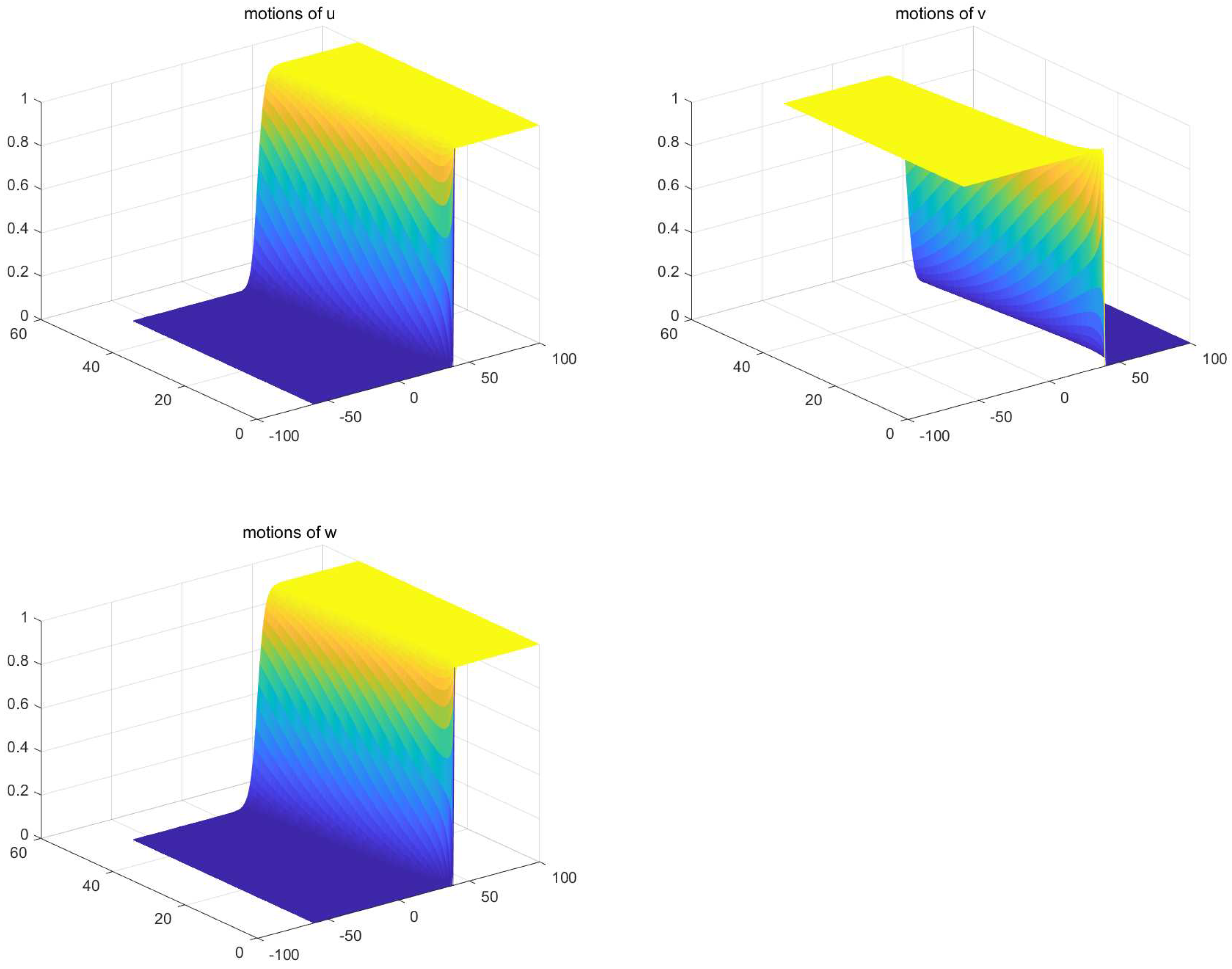
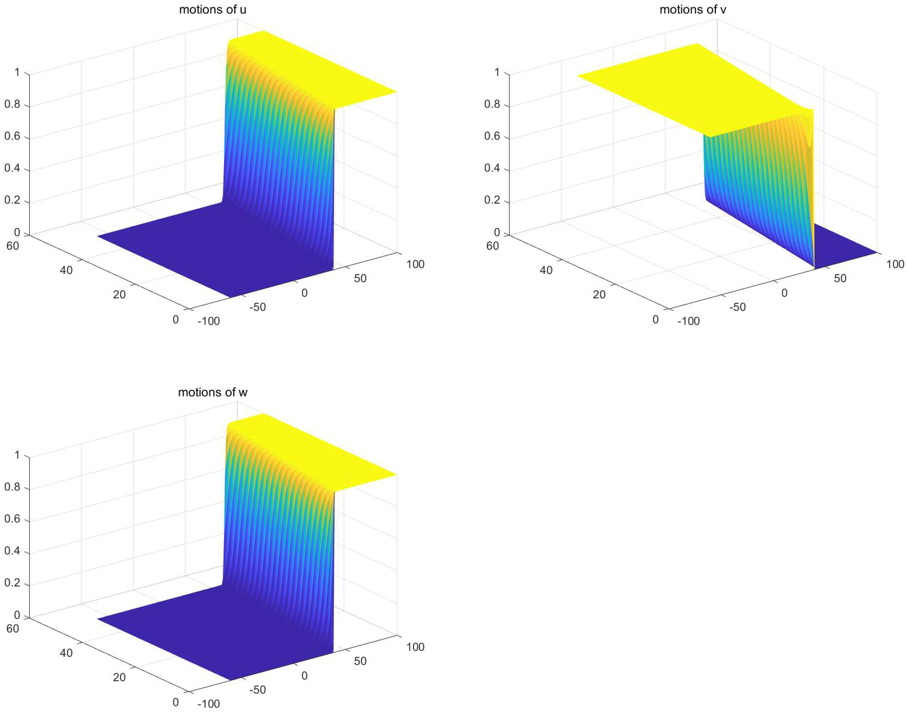
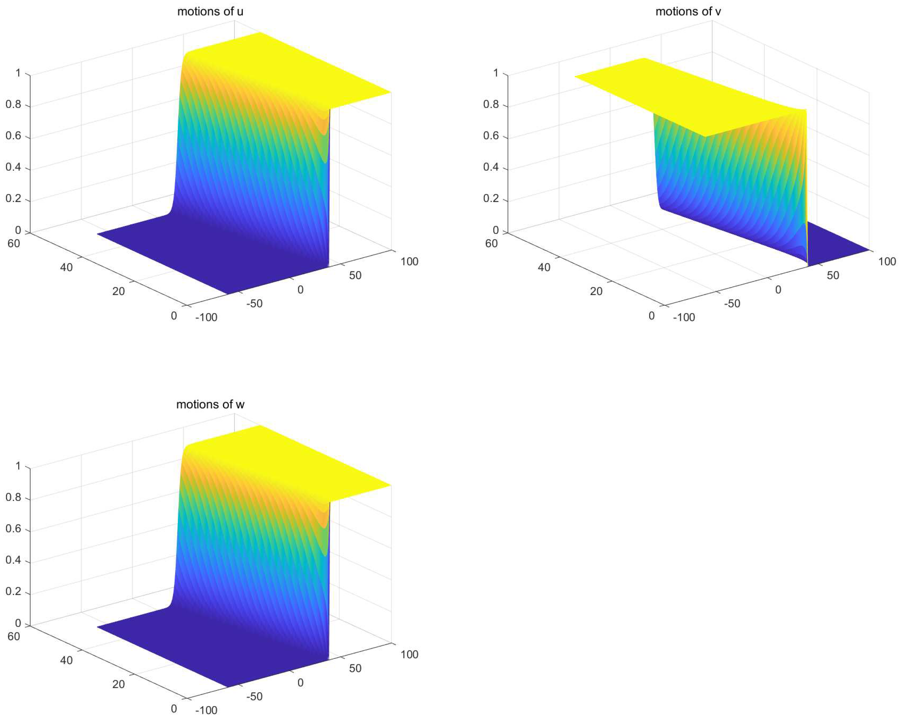
5. Numerical Simulation

We can derive that the bistable wave speed is negative in Theorem 4, which implies that the bistable wave speed propagates to the right and u and w will win the competition. On the contrary, Theorem 5 ensures that the bistable wave speed is positive, which means that the bistable wave speed propagates to the left and v will win the competition.

In order to illustrate our theoretical results from Corollaries 1 and 2, we choose the initial data in the form of

$$u_j\left(0\right)=\left\{\begin{array}{ccc}& 0,\hfill & \hfill 1\le j\le N_j,\\ & 1,\hfill & \hfill N_j+1\le j\le N_L,\end{array}\right.$$

$$v_j\left(0\right)=\left\{\begin{array}{ccc}& 1,\hfill & \hfill 1\le j\le N_j,\\ & 0,\hfill & \hfill N_j+1\le j\le N_L,\end{array}\right.$$

$$w_j\left(0\right)=\left\{\begin{array}{ccc}& 0,\hfill & \hfill 1\le j\le N_j,\\ & 1,\hfill & \hfill N_j+1\le j\le N_L,\end{array}\right.$$

with the boundary conditions

$$\left\{\begin{array}{cc}& u_1\left(t\right)-u_2\left(t\right)=u_{N_L}\left(t\right)-u_{N_{L-1}}\left(t\right)=0,\hfill \\ & v_1\left(t\right)-v_2\left(t\right)=v_{N_L}\left(t\right)-v_{N_{L-1}}\left(t\right)=0,\hfill \\ & w_1\left(t\right)-w_2\left(t\right)=w_{N_L}\left(t\right)-w_{N_{L-1}}\left(t\right)=0,\hfill \end{array}\right.$$

where $N_j$ and $N_L$ are two integers. In what follows, we will set $x\in [-100,100]$ and $t\in [0,60]$, and the step we take here is $\Delta x=1$ and $\Delta t=0.05$. All of the following simulation of the CPU time is about one second.

In (50), we choose

$$\begin{array}{cc}\hfill & a_{11}=b_{11}=c_{11}=1,a_{12}=1.2,b_{12}=0.8,b_{13}=0.7,\hfill \\ \hfill & c_{12}=1.2,d_1=1,d_2=2,d_3=1.3,r_1=r_2=r_3=1.\hfill \end{array}$$

(56)

From this, we can compute ${\tau }_{10}=0.250,{\chi }_{10}=0.119$. It is easy to see that the set of such chosen parameters make (51)–(54) valid. As a result, one may accept the bistable wave speed to be negative. This fact is exactly verified by the numerical results; see Figure 1.

Figure 1. The simulation of (50) for the setting of (56).

In (50), we choose

$$\begin{array}{cc}\hfill & a_{11}=b_{11}=c_{11}=1,a_{12}=10,b_{12}=1.2,b_{13}=1.2,\hfill \\ \hfill & c_{12}=8,d_1=1,d_2=0.5,d_3=1.2,r_1=r_2=r_3=1.\hfill \end{array}$$

(57)

For the above set of parameters, one can derive that ${\tau }_{20}=2.800$. Meanwhile, they fulfill (51) and (55), so the bistable wave speed would be positive according to Corollary 2. This is demonstrated in Figure 2.

Figure 2. The simulation of (50) for the setting of (57).

We all know that the competitive ability of a strong species will be greater than that of a weak species, indicating that the strong species can wipe out the weak one. However, when more than two species are involved, the outcome may not be that simple. Indeed, Theorem 3.4 in Guo [13] proves that it is possible for two weak species to outcompete a strong species in model (2) under certain conditions. Naturally, we wonder whether the same phenomenon can be observed in model (50). To this end, we choose

$$\begin{array}{cc}\hfill & a_{11}=b_{11}=c_{11}=1,a_{12}=c_{12}=1.1,b_{12}=b_{13}=0.9,\hfill \\ \hfill & r_1=r_2=r_3=1,d_1=d_2=d_3=1.\hfill \end{array}$$

(58)

Figure 3 tells us that such a phenomenon still exists.

Figure 3. The simulation of (50) for the setting of (58).

6. Conclusions

We investigate a time-periodic lattice system modeling the evolution of three competing species in the case that one of the species competes with the other two species for common resources, while there is no competition between these other two species. The focus of the paper is the determination of the sign of bistable traveling wave solution, for which it is a challenging task to find the corresponding sufficient and necessary condition. Noting that the system is monotone, we apply the upper/lower solution method and the comparison principle to successfully establish several sufficient conditions so that one can confirm that the sigh is positive or negative. The results that we obtained here reveal how the periodic fluctuation caused by the season or other factors can have an impact on the competitive outcome for the three species. In particular, we addressed an open problem arose by Guo [13] since the integral method used for a continuous system there cannot be used for a discrete system. To confirm the validity of our results, a numerical simulation was also carried out.

References

- Alhasanat, A.; Ou, C. Minimal-speed selection of traveling waves to the Lotka-Volterra competition model. J. Differ. Equ. 2019, 266, 7357–7378. [Google Scholar] [CrossRef]
- Guo, J.-S.; Lin, Y.-C. The sign of the wave speed for the Lotka-Volterra competition-diffusion system. Comm. Pure Appl. Anal. 2013, 12, 2083–2090. [Google Scholar] [CrossRef]
- Ma, M.; Yue, J.; Huang, Z.; Ou, C. Propagation dynamics of bistable traveling wave to a time-periodic Lotka-Volterra competition model arising in strong competition model: Effect of seasonality. J. Dyn. Differ. Equ. 2022, 35, 1745–1767. [Google Scholar] [CrossRef]
- Ma, M.; Yue, J.; Ou, C. Propagation direction of the bistable travelling wavefront for delayed non-local reaction diffusion equations. Proc. Math. Phys. Eng. Sci. 2019, 475, 20180898. [Google Scholar] [CrossRef]
- Ma, M.; Zhang, Q.; Yue, J.; Ou, C. Bistable wave speed of the Lotka-Volterra competition model. J. Biol. Dyn. 2020, 14, 608–620. [Google Scholar] [CrossRef]
- Wang, H.; Ou, C. Propagation direction of the traveling wave for the Lotka-Volterra competitive lattice system. J. Dyn. Differ. Equ. 2021, 33, 1153–1174. [Google Scholar] [CrossRef]
- Zhang, G.-B.; Zhao, X.-Q. Propagation phenomena for a two-species Lotka-Volterra strong competition system with nonlocal dispersal. Calc. Var. Partial Differ. Equ. 2020, 33, 1–34. [Google Scholar] [CrossRef]
- Guo, J.-S.; Wang, Y.; Wu, C.-H.; Wu, C.-C. The minimal speed of traveling wave solutions for a diffusive three species competition system. Taiwanese J. Math. 2015, 19, 1805–1829. [Google Scholar] [CrossRef]
- Pan, C.; Wang, H.; Ou, C. Invasive speed for a competition-diffusion system with three Species. Discrete Contin. Dyn. Syst. B 2022, 27, 3515–3532. [Google Scholar] [CrossRef]
- Chang, C.-H. The stability of traveling wave solutions for a diffusive competition system of three species. J. Math. Anal. Appl. 2018, 459, 564–576. [Google Scholar] [CrossRef]
- Chen, C.-C.; Hung, L.-C.; Mimura, M.; Ueyama, D. Exact travelling wave solutions of three-species competition–diffusion systems. Discrete Contin. Dyn. Syst. B 2012, 17, 2653–2669. [Google Scholar] [CrossRef]
- Meng, Y.-L.; Zhang, W.-G. Properties of traveling wave fronts for three species Lotka-Volterra system. Qual. Theory Dyn. Syst. 2020, 19, 1–28. [Google Scholar] [CrossRef]
- Guo, J.-S.; Nakamura, K.I.; Ogiwara, T.; Wu, C.-H. The sign of traveling wave speed in bistable dynamics. Discrete Contin. Dyn. Syst. 2020, 40, 3451–3466. [Google Scholar] [CrossRef]
- Zheng, J.-P. The wave speed signs for bistable traveling wave solutions in three species competition-diffusion systems. Appl. Math. Mech. 2021, 42, 1296–1305. [Google Scholar]
- Gao, P.; Wu, S.-H. Qualitative properties of traveling wavefronts for a three-component lattice dynamical system with delay. Electron. J. Differ. Equ. 2019, 34, 1–19. [Google Scholar]
- Guo, J.-S.; Wu, C.-C. The existence of traveling wave solutions for a bistable three-component lattice dynamical system. J. Differ. Equ. 2016, 260, 1445–1455. [Google Scholar] [CrossRef]
- Guo, J.-S.; Nakamura, K.-I.; Ogiwara, T.; Wu, C.-C. Stability and uniqueness of traveling waves for a discrete bistable 3-species competition system. J. Math. Anal. Appl. 2019, 472, 1534–1550. [Google Scholar] [CrossRef]
- Su, T.; Zhang, G.-B. Stability of traveling wavefronts for a three-component Lotka-Volterra competition system on a lattice. Electron. J. Differ. Equ. 2018, 57, 1–16. [Google Scholar]
- Wu, H.-C. A general approach to the asymptotic behavior of traveling waves in a class of three-component lattice dynamical systems. J. Dyn. Differ. Equ. 2016, 28, 317–338. [Google Scholar] [CrossRef]
- Dong, F.-D.; Wang, W.-T.; Wang, J.-B. Asymptotic behavior of traveling waves for a three-component system with nonlocal dispersal and its application. Discrete Contin. Dyn. Syst. 2017, 37, 2150058. [Google Scholar] [CrossRef]
- He, J.; Zhang, G.-B. The minimal speed of traveling wavefronts for a three-component competition system with nonlocal dispersal. Int. J. Biomath. 2021, 14, 2150058. [Google Scholar] [CrossRef]
- Hung, L.-C. Traveling wave solutions of competitive-cooperative Lotka-Volterra systems of three species. Nonlinear Anal. Real World Appl. 2011, 12, 3691–3700. [Google Scholar] [CrossRef]
- Ma, Z.-H.; Wu, X.; Rong, Y. Nonlinear stability of traveling wavefronts for competitive-cooperative Lotka-Volterra systems of three species. Appl. Math. Comput. 2017, 315, 331–346. [Google Scholar] [CrossRef]
- Ma, M.; Huang, Z.; Ou, C. Speed of the traveling wave for the bistable Lotka-Volterra competition Model. Nonlinearity 2019, 32, C3143–C3162. [Google Scholar] [CrossRef]
- Bunimovich, L.A.; Sinai, Y.G. Spacetime chaos in coupled map lattices. Nonlinearity 1988, 1, 491. [Google Scholar] [CrossRef]
- Chow, S.N. Lattice dynamical systems. In Dynamical Systems; Lecture Notes in Mathematics; Macki, J.W., Zecca, P., Eds.; Springer: Berlin, Germany, 2003; Volume 1822, pp. 1–102. [Google Scholar]
- Fife, P.C. Mathematical Aspects of Reacting and Diffusing Systems; Lecture Notes in Biomathematics; Springer: Berlin, Germany, 1979; Volume 28. [Google Scholar]
- Guo, J.-S.; Wu, C.-H. Wave propagation for a two-component lattice dynamical system arising in strong competition models. J. Differ. Equ. 2011, 250, 3504–3533. [Google Scholar] [CrossRef]
- Vukusic, P.; Sambles, J.R. Photonic structures in biology. Nature 2003, 424, 852–855. [Google Scholar] [CrossRef]
- Wang, H.; Pan, C. Spreading speed of a lattice time-periodic Lotka-Volterra competition system with bistable nonlinearity. Appl. Anal. 2022, 102, 4757–4778. [Google Scholar] [CrossRef]
- Chen, X.; Guo, J.-S.; Wu, C.-C. Traveling waves in discrete periodic media for bistable dynamics. Arch. Ration. Mech. Anal. 2008, 189, 189–236. [Google Scholar] [CrossRef]
- Fang, J.; Zhao, X.-Q. Bistable traveling waves for monotone semiflows with applications. J. Eur. Math. Soc. 2011, 17, 2243–2288. [Google Scholar] [CrossRef]
- Ma, M.; Ou, C. Asymptotic analysis of the perturbed Poisson-Boltzmann equation on un bounded domains. Asymptot. Anal. 2015, 91, 125–146. [Google Scholar]
- Bao, X.; Wang, Z.-C. Existence and stability of time periodic traveling waves for a periodic bistable Lotka-Volterra competition system. J. Differ. Equ. 2013, 255, 2402–2435. [Google Scholar] [CrossRef]
- Thieme, H.R. Asymptotic estimates of the solutions of nonlinear integral equations and asymptotic speeds for the spread of populations. J. Reine Ang. Math. 1979, 306, 94–121. [Google Scholar]
Disclaimer/Publisher’s Note: The statements, opinions and data contained in all publications are solely those of the individual author(s) and contributor(s) and not of MDPI and/or the editor(s). MDPI and/or the editor(s) disclaim responsibility for any injury to people or property resulting from any ideas, methods, instructions or products referred to in the content. |
© 2024 by the authors. Licensee MDPI, Basel, Switzerland. This article is an open access article distributed under the terms and conditions of the Creative Commons Attribution (CC BY) license (https://creativecommons.org/licenses/by/4.0/).