Efficient Solutions for Stochastic Fractional Differential Equations with a Neutral Delay Using Jacobi Poly-Fractonomials

Abstract

This paper introduces a novel numerical technique for solving fractional stochastic differential equations with neutral delays. The method employs a stepwise collocation scheme with Jacobi poly-fractonomials to consider unknown stochastic processes. For this purpose, the delay differential equations are transformed into augmented ones without delays. This transformation makes it possible to use a collocation scheme improved with Jacobi poly-fractonomials to solve the changed equations repeatedly. At each iteration, a system of nonlinear equations is generated. Next, the convergence properties of the proposed method are rigorously analyzed. Afterward, the practical utility of the proposed numerical technique is validated through a series of test examples. These examples illustrate the method’s capability to produce accurate and efficient solutions.

1. Introduction

Ordinary differential equations (ODEs) are fundamental mathematical tools used to determine deterministic dynamical systems’ evolution by describing a relationship between the state variables and their rates of change [1]. They are essential for understanding phenomena such as motion [2], electrical circuits [3], and structural mechanics [4]. In real-world phenomena, dynamical systems are often influenced by external noise or inherent randomness, typically represented by Brownian motion, making them difficult to model with ordinary differential equations (ODEs). Stochastic differential equations (SDEs) are introduced as an extension to ODEs in order to incorporate random processes and effectively capture random fluctuations. For example, in finance, SDEs model the random behavior of market prices and interest rates, providing insights into pricing financial instruments and managing risk [5,6,7,8]. In engineering, SDEs assist in designing systems that can withstand random environmental disturbances [9,10]. In population dynamics, they model the effects of random events on species populations [11,12], and in biology, they describe processes such as gene expression and the spread of diseases [13,14,15,16].

Delay differential equations (DDEs) are a class of differential equations used to model dynamical systems that depend on past states, meaning that the current rate of change of the system’s state is a function of the current state and its history. The applications of time-delay systems are vast, ranging from engineering [17], where they model network-induced delays in control systems, to economics [18], where they represent the lag between investment and return, and to biology [19], where they can model the spread of diseases or population dynamics. Delays can be constant, time-varying, or distributed, and they are inherent in many real-world processes due to the finite speed of information transmission [20], material transport delays [18,20], or gestation periods in biological systems [19]. Time delays can lead to complex behaviors such as increased oscillatory tendencies, instability, and bifurcations, posing significant challenges in such systems’ analysis, control, and stability [21].

Fractional differential equations (FDEs) are developed by the presence of derivatives and integrals of non-integer order, known as fractional calculus, which generalizes the concept of integer-order differentiation and integration to arbitrary order. Fractional derivatives provide an excellent tool for describing memory and the hereditary properties of various materials and processes [22]. Unlike classical derivative operators, fractional derivatives are non-local, encapsulating effects over an interval, which makes them inherently suitable for modeling systems with memory and spatial heterogeneity [23,24,25]. Non-locality and the ability to capture long-term memory make fractional systems a natural choice for describing complex phenomena in control theory [26,27], biology [28], and finance [29], where processes are influenced by their entire history rather than just their current state. This is particularly useful in fields such as viscoelasticity [24], where materials exhibit both viscous and elastic characteristics, and in anomalous diffusion, where particle trajectories deviate from classical Brownian motion.

Stochastic fractional delay differential equations (SFDDEs) significantly advance the modeling of complex dynamical real-world problems by incorporating the system’s past, possible random processes, and hereditary properties. This class of differential equations has garnered substantial attention from researchers due to its potential to capture the intricate interplay of randomness and memory effects in dynamic systems. For instance, recent studies have delved into the uniqueness and solvability of FSDEs with constant delay [30], proposed collocation methods for solving nonlinear fractional SDEs with constant delay [31,32,33], and considered approximation techniques for solutions of neutral delay fractional SDEs based on the Faedo–Galerkin method [34]. Additionally, the numerical solution of neutral stochastic integro-differential equations with Caputo fractional derivatives has been explored [35], and innovative approaches such as the least squares support vector regression method based on Chelyshkov polynomials have been presented to solve a class of nonlinear SDEs with variable fractional Brownian motion [36]. While the foundational methods are well-established, considerable challenges emerge when neutral DDEs are augmented with fractional derivatives and stochastic terms. Even in basic fractional DDEs, the nonlocal nature of fractional operators causes the numerical errors in explicit finite-difference methods to increase exponentially. Nonetheless, as shown in various studies, these challenges can be effectively mitigated using spectral methods [37,38].

This paper proposes a stepwise collocation scheme incorporating Jacobi poly-fractonomials, a more generalized form of Jacobi polynomials, to obtain the numerical solution of a class of stochastic fractional neutral delay differential equations (SFDDEs) containing neutral delays, which is referred to as SFNDEs. Moreover, Jacobi polynomials form a versatile family of orthogonal polynomials from which several well-known polynomials may be derived through the appropriate specification of parameters or limits. Well-known examples are Legendre polynomials with a zero value for both of the parameters, Gegenbauer (ultra-spherical) polynomials for which the parameters are equal, and Chebyshev polynomials of the first and second kinds corresponding to specific values of the parameters. Besides these, Laguerre and Hermite polynomials can also be transformed into Jacobi polynomials, though not as direct examples. Jacobi poly-fractonomials provide a robust structure for representing intricate systems characterized by fractional-order dynamics. The specific features of these models make them a necessary addition to the mathematical toolbox for extending the capability provided to analysts and researchers working in fields where fractional-order models see widespread application. While they entail a bit more complexity relative to the integer-order polynomials, such difficulties are often overshadowed by their potential for much better modeling and for investigating subtle behaviors in fractional-order systems, both of which are shown in this study. The approach begins by transforming the equations into equivalent delay-free forms. Then, the collocation scheme is iteratively applied to generate a set of nonlinear equations at each stage, which can be solved by a common nonlinear solver. The convergence of the proposed method is studied, and its efficiency is shown in a set of test examples. The organization of this paper is as follows: In Section 2, the fundamental definitions and characteristics necessary for understanding the subsequent topics are elaborated upon. The class of SFDDEs of interest in this study is introduced in Section 3. Section 4 discusses the stepwise Jacobi poly-fractonomials collocation scheme. A thorough analysis of the error associated with this scheme is provided in Section 5. The numerical algorithm for two test examples is explained in detail in Section 6. Finally, Section 7 presents the concluding remarks of this article.

2. Preliminaries and Definitions

This section presents essential principles of fractional definitions and the characteristics of Jacobi polynomials, including the definition associated with fractional types.

Definition 1

([22]). The Riemann–Liouville fractional integral of order η is a generalization of the classical integral and is defined as

$$\begin{array}{c}\hfill {\mathrm{I}}_t^{\eta }u\left(t\right)={\displaystyle \frac{1}{\Gamma \left(\eta \right)}}{\int }_0^t{(t-s)}^{\eta -1}u\left(s\right)\mathrm{d}s,(\eta ,t>0),\end{array}$$

(1)

where $\Gamma \left(\eta \right)$ denotes the Gamma function, which is a continuous extension of the factorial function to non-integer values.

Definition 2

([22]). The Caputo fractional derivative of order $\eta \in (0,1]$, denoted by ${}^{\mathrm{C}}\mathcal{D}_t^{\eta }[·]$, provides a modification of the traditional derivative by incorporating fractional calculus principles. That is,

$$\begin{array}{cc}\hfill {}^{\mathrm{C}}\mathcal{D}_t^{\eta }u\left(t\right)& ={\displaystyle \frac{1}{\Gamma (1-\eta )}}{\int }_0^t{(t-s)}^{-\eta }{u}^{\prime }\left(s\right)\mathrm{d}s,\eta \in (0,1].\hfill \end{array}$$

(2)

Definition 3

([39]). The Jacobi polynomial ${\varphi }_i^{(\beta ,\gamma )}\left(t\right)$ of degree i satisfies the following explicit form:

$${\varphi }_i^{(\beta ,\gamma )}\left(t\right)={\displaystyle \sum _{k=0}^i}{\Pi }_{k,i}^{(\beta ,\gamma )}{\left({\displaystyle \frac{t+1}{2}}\right)}^k,(\beta ,\gamma >-1),$$

(3)

where

$${\Pi }_{k,i}^{(\beta ,\gamma )}:={\displaystyle \frac{{(-1)}^{i-k}\Gamma (i+\gamma +1)\Gamma (i+\beta +\gamma +k+1)}{(i-k)!k!\Gamma (k+\gamma +1)\Gamma (i+\beta +\gamma +1)}}.$$

Definition 4

([40,41]). The Jacobi poly-fractonomial ${\theta }_i^{\mu }\left(t\right)$ over $[-1,1]$ is defined by

$${\theta }_i^{\mu }\left(t\right)={(t+1)}^{\mu }{\varphi }_{i-1}^{(-\mu ,\mu )}\left(t\right),i\ge 1,$$

(4)

where the Jacobi polynomial ${\varphi }_{i-1}^{(-\mu ,\mu )}\left(t\right)$ is defined in Equation (3) when $\mu \in (0,1)$.

Lemma 1

([41]). The Jacobi poly-fractonomials ${\theta }_i^{\mu }\left(t\right)$ are orthogonal using the weight function

$$\mathbf{w}\left(t\right)={(1-t)}^{-\mu }{(1+t)}^{-\mu },$$

(5)

such that

$${\int }_{-1}^1\mathbf{w}\left(t\right){\theta }_i^{\left(\mu \right)}\left(t\right){\theta }_j^{\left(\mu \right)}\left(t\right)\mathrm{d}t={\varrho }_i^{(-\mu ,\mu )}{\delta }_{i,j},$$

and

$${\varrho }_i^{(-\mu ,\mu )}={\int }_{-1}^1{(1-t)}^{-\mu }{(1+t)}^{\mu }{\left({\varphi }_i^{(-\mu ,\mu )}\left(t\right)\right)}^2\mathrm{d}t={\displaystyle \frac{2\Gamma (i-\mu )\Gamma (i+\mu )}{(2i-1)(i-1)!\Gamma \left(i\right)}},$$

where ${\delta }_{i,j}$ is the kronecker function.

Definition 5

([40]). The shifted Gauss–Lobatto–Chebyshev (GLC) quadrature nodes over $[{\mathit{e}}_1,{\mathit{e}}_2]$ are

$$\begin{array}{c}\hfill {}_{{\mathit{e}}_1}{}^{{\mathit{e}}_2}{\mathit{t}}_i={\displaystyle \frac{{\mathit{e}}_2-{\mathit{e}}_1}{2}}({\mathit{z}}_i+1)+{\mathit{e}}_1,i=1,\dots ,n+1,\end{array}$$

(6)

where ${\mathit{z}}_i=cos\left({\displaystyle \frac{\pi }{2}}{\displaystyle \frac{2i-1}{n+1}}\right)$, $i=1,\dots ,n+1$.

Definition 6

([32]). The shifted Jacobi poly-fractonomials, denoted as ${\theta }_i^{\mu }(t;{\mathit{e}}_1,{\mathit{e}}_2)$, are a specific class of polynomials defined over the interval $[{\mathit{e}}_1,{\mathit{e}}_2]$. These polynomials are formulated by shifting the standard Jacobi polynomials to the desired interval. Namely,

$${\theta }_i^{\mu }(t;{\mathit{e}}_1,{\mathit{e}}_2)={\theta }_i^{\mu }\left({\displaystyle \frac{2}{{\mathit{e}}_2-{\mathit{e}}_1}}(t-{\mathit{e}}_1)-1\right),i\ge 1,$$

where t is the variable, ${\mathit{e}}_1$ and ${\mathit{e}}_2$ represent the endpoints of the interval, and μ is a parameter associated with the poly-fractonomials. This transformation effectively maps the interval $[{\mathit{e}}_1,{\mathit{e}}_2]$ to the standard interval $[-1,1]$, facilitating the use of Jacobi polynomials in various applications.

Lemma 2

([40]). Let $\Omega :=[{\mathit{e}}_1,{\mathit{e}}_2]$ and the function space ${\mathbf{L}}_{\gamma ,\delta }^2(\Omega )$ be defined as follows:

$${\mathbf{L}}_{\gamma ,\delta }^2(\Omega )=\left\{{g:g\mathit{is}\mathit{measurable}\mathit{and}\parallel g\parallel }_{{\mathbf{L}}_{\gamma ,\delta }^2(\Omega )}<\infty \right\},$$

where

$$\begin{array}{c}\hfill {\parallel g\parallel }_{{\mathbf{L}}_{\gamma ,\delta }^2(\Omega )}={\left({\int }_{\Omega }{\mathbf{w}}^{\gamma ,\delta }(\zeta ;{\mathit{e}}_1,{\mathit{e}}_2){\left|g\left(\zeta \right)\right|}^2\mathrm{d}\zeta \right)}^{{\displaystyle \frac{1}{2}}},\end{array}$$

with the weight function ${\mathbf{w}}^{\gamma ,\delta }(t;{\mathit{e}}_1,{\mathit{e}}_2)={({\mathit{e}}_2-t)}^{\gamma }{(t-{\mathit{e}}_1)}^{\delta }$, $\gamma ,\delta >-1$ [40,42]. In addition, let

$$\begin{array}{cc}\hfill {\Lambda }_{\gamma ,\delta }^m(\Omega )& :=\left\{g:{\partial }_t^{r}g\in {\mathbf{L}}_{\gamma +r,\delta +r}^2(\Omega ),r=0,1,\dots ,m\right\},\hfill \\ \hfill {\mathbf{B}}_{\gamma ,-\delta }^q(\Omega )& :=\left\{g:{\mathcal{D}}_t^{\delta +r}g\in {\mathbf{L}}_{\gamma +\delta +r,r}^2(\Omega ),r=0,1,\dots ,q\right\}.\hfill \end{array}$$

For $g\in {\mathbf{L}}_{-\mu ,-\mu }^2(\Omega )$, then the function $g\left(t\right)$ can be approximated as follows:

$$g\left(t\right)\simeq g_n\left(t\right)={\displaystyle \sum _{r=1}^{n+1}}{\mathtt{c}}_r{\theta }_r^{\left(\mu \right)}(t;{\mathit{e}}_1,{\mathit{e}}_2)\triangleq {\mathbf{C}}^{\mathrm{T}}{}_{{\mathit{e}}_1}{}^{{\mathit{e}}_2}\Theta \left(t\right),$$

(7)

where

$$\begin{array}{cc}\hfill {\mathtt{c}}_r& ={\displaystyle \frac{1}{{\psi }_r}}{\int }_{\Omega }g\left(t\right){\mathbf{w}}^{-\mu ,-\mu }(t;{\mathit{e}}_1,{\mathit{e}}_2){\theta }_r^{\left(\mu \right)}(t;{\mathit{e}}_1,{\mathit{e}}_2)\mathrm{d}t,\hfill \\ \hfill {\psi }_r& :={\displaystyle \frac{({\mathit{e}}_2-{\mathit{e}}_1)\Gamma (r-\mu +1)\Gamma (r+\mu +1)}{(2r+1){\Gamma }^2(r+1)}},\hfill \\ \hfill \mathbf{C}& :={\left[{\mathtt{c}}_1,{\mathtt{c}}_2,\cdots ,{\mathtt{c}}_{n+1}\right]}^{\mathrm{T}},\hfill \\ \hfill {}_{{\mathit{e}}_1}{}^{{\mathit{e}}_2}\Theta \left(t\right)& :={\left[{\theta }_1^{\left(\mu \right)}(t;{\mathit{e}}_1,{\mathit{e}}_2),\cdots ,{\theta }_{n+1}^{\left(\mu \right)}(t;{\mathit{e}}_1,{\mathit{e}}_2)\right]}^{\mathrm{T}}.\hfill \end{array}$$

Lemma 3

([43]). If $g\left(t\right)\in {\mathbf{C}}^{2\overline{\mathrm{P}}}(\Omega )$, where $\Omega :=[{\mathit{e}}_1,{\mathit{e}}_2]$, then an approximate integral of the function $g\left(t\right)$ over the interval $\Omega$ can be obtained using the Legendre–Gauss quadrature formula:

$${\int }_{{\mathit{e}}_1}^{{\mathit{e}}_2}g\left(s\right)\mathrm{d}s\simeq {\displaystyle \frac{{\mathit{e}}_2-{\mathit{e}}_1}{2}}{\displaystyle \sum _{i=0}^{\overline{\mathrm{P}}}}{\omega }_{i}g\left({\displaystyle \frac{{\mathit{e}}_2-{\mathit{e}}_1}{2}}{\sigma }_i+{\displaystyle \frac{{\mathit{e}}_2+{\mathit{e}}_1}{2}}\right),$$

(8)

where $\{{\sigma }_i:i=0,\dots ,\overline{\mathrm{P}}\}$ are the zeros of the Legendre polynomial ${\varphi }_{\overline{\mathrm{P}}+1}^{(0,0)}\left(t\right)$, and the corresponding Legendre–Gauss weights $\{{\omega }_i:i=0,\dots ,\overline{\mathrm{P}}\}$ are given by

$${\omega }_i={\displaystyle \frac{2}{(1-{\sigma }_i^2){\left({\partial }_t\left[{\varphi }_{\overline{\mathrm{P}}+1}^{(0,0)}\right]\left({\sigma }_i\right)\right)}^2}}.$$

Lemma 4

([44,45]). Let $g\left(t\right)$, for $t\in \Omega$, be a stochastic process. The It$\widehat{o}$ integral of $g\left(t\right)$ over the interval $\Omega$ is defined as

$${\int }_{{\mathit{e}}_1}^{{\mathit{e}}_2}g\left(s\right)\mathrm{d}{\mathcal{B}}_s={\displaystyle \sum _{i=0}^{\overline{\mathrm{M}}-1}}g\left({\varsigma }_i\right)\left\{\mathcal{B}\left({\varsigma }_{i+1}\right)-\mathcal{B}\left({\varsigma }_i\right)\right\}+{\mathcal{R}}_{It\widehat{o}},$$

(9)

where the points ${\varsigma }_i$ are defined by

$${\varsigma }_i={\mathit{e}}_1+{\displaystyle \frac{{\mathit{e}}_2-{\mathit{e}}_1}{\overline{\mathrm{M}}}}i,i=0,1,\cdots ,\overline{\mathrm{M}}.$$

$\mathcal{B}\left(t\right)$ denotes the standard Brownian motion, and ${\mathcal{R}}_{It\widehat{o}}$ represents the remainder term of the It$\widehat{o}$ integral approximation. The remainder term ${\mathcal{R}}_{It\widehat{o}}$ becomes negligible in the mean square sense as the number of subdivisions $\overline{\mathrm{M}}$ approaches infinity. Specifically, the expectation of the squared norm of the remainder term, $\mathbb{E}\left[|{\mathcal{R}}_{It\widehat{o}}{|}^2\right]$, tends to zero as $\overline{\mathrm{M}}\to \infty$, ensuring that the approximation converges to the true It$\widehat{o}$ integral.

3. Problem Statement

This paper studies the following stochastic fractional delay differential equation with a natural delay (SFNDE):

$$\begin{array}{cc}\hfill {}^{\mathrm{C}}\mathcal{D}_t^{\eta }[u\left(t\right)& -\mathfrak{f}\left(u(t-\alpha (t\left)\right)\right)]\hfill \\ \hfill & =\mathcal{P}(u\left(t\right),u(t-\alpha \left(t\right)))+\mathcal{H}(u\left(t\right),u(t-\alpha \left(t\right))){\dot{\mathcal{B}}}_t,t\in (0,\mathtt{T}],\hfill \end{array}$$

(10)

subject to the initial condition

$$\begin{array}{cc}\hfill u\left(t\right)& =\phi \left(t\right),t\in [-\tau ,0],\hfill \end{array}$$

(11)

where the continuous function $\alpha \left(t\right):[0,\mathtt{T}]\to [0,\tau ]$ is a Borel measurable function for the positive constant $\tau$, and $\mathcal{P}$, $\mathcal{H}$, and $\mathfrak{f}$ are Borel measurable functions satisfying in the following Lipschitz conditions:

$$\begin{array}{cc}\hfill |\mathfrak{f}\left(u\right)-\mathfrak{f}\left(\overline{u}\right)|& \le \widehat{\varsigma }|u-\overline{u}|,\hfill \end{array}$$

(12a)

$$\begin{array}{cc}\hfill |\mathcal{P}(u,v)-\mathcal{P}(\overline{u},\overline{v})|& \le \check{\mu }|u-\overline{u}|+\widehat{\mu }|v-\overline{v}|,\hfill \end{array}$$

(12b)

$$\begin{array}{cc}\hfill |\mathcal{H}(u,v)-\mathcal{H}(\overline{u},\overline{v})|& \le \check{\delta }|u-\overline{u}|+\widehat{\delta }|v-\overline{v}|,\hfill \end{array}$$

(12c)

where $\widehat{\varsigma },\check{\mu },\widehat{\mu },\check{\delta },\widehat{\delta }\in {\mathbb{R}}^{+}$, $\mathtt{T}\in (0,+\infty )$, the stochastic process $\mathcal{B}\left(t\right)$ on $t\in [0,\mathtt{T}]$ denotes standard Brownian motion on a complete probability space $\left(\Omega ,\mathcal{F},{\left\{{\mathcal{F}}_t\right\}}_{t\in [0,\mathtt{T}]},\mathbb{P}\right)$ with a filtration ${\left\{{\mathcal{F}}_t\right\}}_{t\in [0,\mathtt{T}]}$ satisfying the usual conditions, i.e., ${\dot{\mathcal{B}}}_t:={\displaystyle \frac{\mathrm{d}\mathcal{B}\left(t\right)}{\mathrm{d}t}}$, and $u\left(t\right)$ is an unknown stochastic process to be determined.

According to Definition 1, the stochastic fractional neutral delay differential Equation (SFNDE) given by Equation (10) can be transformed into its equivalent integral form as

$$\begin{array}{cc}\hfill u\left(t\right)=u_0& +\mathfrak{f}\left(u(t-\alpha (t\left)\right)\right)+{\displaystyle \frac{1}{\Gamma \left(\eta \right)}}{\int }_0^t{(t-s)}^{\eta -1}\mathcal{P}(u\left(s\right),u(s-\alpha \left(s\right)))\mathrm{d}s\hfill \\ \hfill & +{\displaystyle \frac{1}{\Gamma \left(\eta \right)}}{\int }_0^t{(t-s)}^{\eta -1}\mathcal{H}(u\left(s\right),u(s-\alpha \left(s\right)))\mathrm{d}{\mathcal{B}}_s,\hfill \end{array}$$

(13)

where the initial value $u_0$ is

$$u_0:=\phi \left(0\right)-\mathfrak{f}\left(\phi (-\alpha (0\left)\right)\right).$$

4. Stepwise Jacobi Poly-Fractonomials Collocation Scheme

To approximate the numerical solution of the integral Equation (13), the first step involves converting this time-varying delay stochastic neutral integral equation into an equivalent non-delay stochastic neutral integral equation. This transformation is achieved using a stepwise method. The approach involves dividing the entire interval $[0,\mathtt{T}]$ into smaller subintervals of length $\tau$. The delay term $\alpha \left(t\right)$ is approximated within each subinterval, effectively transforming the original time-varying delay problem into a series of non-delay problems. The collocation method, utilizing Jacobi poly-fractonomials, is then applied to each subinterval ${\Omega }_k$.

Let $\tau =\underset{t\in [0,\mathtt{T}]}{max}\left\{\alpha \left(t\right)\right\}$, and let $\mathtt{p}$$=⌊{\displaystyle \frac{\mathtt{T}}{\tau }}⌋$. The goal is to find the numerical solution of Equation (13), subject to the condition (11), within any subinterval ${\Omega }_k:=[(k-1)\tau ,k\tau ]$, for $k=1,\dots ,\mathtt{p}$, by employing a collocation technique based on Jacobi poly-fractonomials. Moreover, in the first step, Equation (13) is equivalent to

$$\begin{array}{cc}\hfill u^1\left(t\right)& =u_0+\mathfrak{f}\left(u^0(t-\alpha \left(t\right))\right)\hfill \\ \hfill & +{\displaystyle \frac{1}{\Gamma \left(\eta \right)}}{\int }_0^t{(t-s)}^{\eta -1}\mathcal{P}(u^1\left(s\right),u^0(s-\alpha \left(s\right)))\mathrm{d}s\hfill \\ \hfill & +{\displaystyle \frac{1}{\Gamma \left(\eta \right)}}{\int }_0^t{(t-s)}^{\eta -1}\mathcal{H}(u^1\left(s\right),u^0(s-\alpha \left(s\right)))\mathrm{d}{\mathcal{B}}_s,\hfill \end{array}$$

(14)

where $u^0\left(t\right)=\phi \left(t\right)$.

An approximate solution of $u\left(t\right)$ in the first interval can be derived using the results presented in Lemma 2. That is,

$$u^1\left(t\right)\simeq u_n^1\left(t\right)={\displaystyle \sum _{r=1}^{n+1}}{\mathtt{c}}_r^1{\theta }_r^{\left(\mu \right)}(t;0,\tau )\triangleq {\mathbf{C}}_1^{\mathrm{T}}{}_0{}^{\tau }\Theta \left(t\right),$$

(15)

where ${\mathbf{c}}_1={\left[{\mathtt{c}}_1^1,{\mathtt{c}}_2^1,\dots ,{\mathtt{c}}_{n+1}^1\right]}^{\mathrm{T}}$.

Using this approximation in Equation (14) provides the following result:

$$\begin{array}{cc}\hfill {\mathbf{C}}_1^{\mathrm{T}}{}_0{}^{\tau }\Theta \left(t\right)& \simeq u_0+\mathfrak{f}\left(u_n^0(t-\alpha \left(t\right))\right)\hfill \\ \hfill & +{\displaystyle \frac{1}{\Gamma \left(\eta \right)}}{\int }_0^t{(t-s)}^{\eta -1}\mathcal{P}({\mathbf{C}}_1^{\mathrm{T}}{}_0{}^{\tau }\Theta \left(t\right)\left(s\right),u_n^0(s-\alpha \left(s\right)))\mathrm{d}s\hfill \\ \hfill & +{\displaystyle \frac{1}{\Gamma \left(\eta \right)}}{\int }_0^t{(t-s)}^{\eta -1}\mathcal{H}({\mathbf{C}}_1^{\mathrm{T}}{}_0{}^{\tau }\Theta \left(s\right),u_n^0(s-\alpha \left(s\right)))\mathrm{d}{\mathcal{B}}_s,\hfill \end{array}$$

(16)

where

$$\begin{array}{cc}\hfill u^0\left(t\right)& \simeq u_n^0\left(t\right)={\displaystyle \sum _{r=1}^{n+1}}{\mathtt{c}}_r^0{\theta }_r^{\left(\mu \right)}(t;-\tau ,0)\triangleq {\mathbf{C}}_0^{\mathrm{T}}{}_{-\tau }{}^0\Theta \left(t\right),\hfill \\ \hfill {\mathtt{c}}_r^0& ={\displaystyle \frac{1}{{\psi }_r}}{\int }_{\Omega }\phi \left(t\right){\mathbf{w}}^{-\mu ,-\mu }(t;-\tau ,0){\theta }_r^{\left(\mu \right)}(t;-\tau ,0)\mathrm{d}t.\hfill \end{array}$$

(17)

Now, the CGL points $\mathbf{t}_i^1:={}_{\tau }{}^0{\mathbf{t}}_i$, as defined in Definition 5, are utilized in Equation (17), which results in

$$\begin{array}{cc}\hfill {\mathbf{C}}_1^{\mathrm{T}}{}_0{}^{\tau }\Theta \left({\mathbf{t}}_i^1\right)& =u_0+\mathfrak{f}\left(u_n^0({\mathbf{t}}_i^1-\alpha \left({\mathbf{t}}_i^1\right))\right)\hfill \\ \hfill & +{\displaystyle \frac{1}{\Gamma \left(\eta \right)}}{\int }_0^{{\mathbf{t}}_i^1}{({\mathbf{t}}_i^1-s)}^{\eta -1}\mathcal{P}({\mathbf{C}}_1^{\mathrm{T}}{}_0{}^{\tau }\Theta \left(s\right),u_n^0(s-\alpha \left(s\right)))\mathrm{d}s\hfill \\ \hfill & +{\displaystyle \frac{1}{\Gamma \left(\eta \right)}}{\int }_0^{{\mathbf{t}}_i^1}{({\mathbf{t}}_i^1-s)}^{\eta -1}\mathcal{H}({\mathbf{C}}_1^{\mathrm{T}}{}_0{}^{\tau }\Theta \left(s\right),u_n^0(s-\alpha \left(s\right)))\mathrm{d}{\mathcal{B}}_s.\hfill \end{array}$$

(18)

Utilizing the Legendre–Gauss integration method as described in Lemma 3, along with the It$\widehat{o}$ approximation detailed in Lemma 4 for the integral components of Equation (18), yields

$$\begin{array}{c}{\int }_0^{{\mathbf{t}}_i^1}({\mathbf{t}}_i^1{-s)}^{\eta -1}\mathcal{P}({\mathbf{C}}_1^{\mathrm{T}}{}_0{}^{\tau }\Theta \left(s\right),u_n^0(s-\alpha \left(s\right)))\mathrm{d}s\hfill \\ \hfill ={\displaystyle \frac{{\mathbf{t}}_i^1}{2}}{\displaystyle \sum _{j=0}^{\overline{\mathrm{P}}}}{\omega }_j{({\mathbf{t}}_i^1-{\nu }_{i,j}^1)}^{\eta -1}\mathcal{P}\left({\mathbf{C}}_1^{\mathrm{T}}{}_0{}^{\tau }\Theta \left({\nu }_{i,j}^1\right),u_n^0\left({\nu }_{i,j}^1-\alpha \left({\nu }_{i,j}^1\right)\right)\right),\end{array}$$

(19)

$$\begin{array}{c}{\int }_0^{{\mathbf{t}}_i^1}({\mathbf{t}}_i^1{-s)}^{\eta -1}\mathcal{H}({\mathbf{C}}_1^{\mathrm{T}}{}_0{}^{\tau }\Theta \left(s\right),u_n^0(s-\alpha \left(s\right)))\mathrm{d}{\mathcal{B}}_s\hfill \\ \hfill ={\displaystyle \sum _{j=0}^{\overline{\mathrm{M}}-1}}{({\mathbf{t}}_i^1-{\varsigma }_{i,j}^1)}^{\eta -1}\mathcal{H}\left({\mathbf{C}}_1^{\mathrm{T}}{}_0{}^{\tau }\Theta \left({\varsigma }_{i,j}^1\right),u_n^0({\varsigma }_{i,j}^1-\alpha \left({\varsigma }_{i,j}^1\right))\right)\\ \times \{\mathcal{B}\left({\varsigma }_{i,j+1}^1\right)-\mathcal{B}\left({\varsigma }_{i,j}^1\right)\},\hfill \end{array}$$

(20)

where

$${\nu }_{i,j}^1={\displaystyle \frac{{\mathbf{t}}_i^1}{2}}{\sigma }_j+{\displaystyle \frac{{\mathbf{t}}_i^1}{2}},j=0,1,\dots ,\overline{\mathrm{P}},{\varsigma }_{i,j}^1={\displaystyle \frac{{\mathbf{t}}_i^1}{\overline{\mathrm{M}}}}j,j=0,1,\dots ,\overline{\mathrm{M}}.$$

Finally, Equations (18)–(20) give the following system of nonlinear equations:

$$\begin{array}{cc}\hfill {\mathbf{C}}_1^{\mathrm{T}}{}_0{}^{\tau }\Theta \left({\mathbf{t}}_i^1\right)& =u_0+\mathfrak{f}\left(u_n^0({\mathbf{t}}_i^1-\alpha \left({\mathbf{t}}_i^1\right))\right)\hfill \\ \hfill & +{\displaystyle \frac{{\mathbf{t}}_i^1}{2\Gamma \left(\eta \right)}}{\displaystyle \sum _{j=0}^{\overline{\mathrm{P}}}}{\omega }_j{({\mathbf{t}}_i^1-{\nu }_{i,j}^1)}^{\eta -1}\mathcal{P}\left({\mathbf{C}}_1^{\mathrm{T}}{}_0{}^{\tau }\Theta \left({\nu }_{i,j}^1\right),u_n^0\left({\nu }_{i,j}^1-\alpha \left({\nu }_{i,j}^1\right)\right)\right)\hfill \\ \hfill & +{\displaystyle \frac{1}{\Gamma \left(\eta \right)}}{\displaystyle \sum _{j=0}^{\overline{\mathrm{M}}-1}}{({\mathbf{t}}_i^1-{\varsigma }_{i,j}^1)}^{\eta -1}\mathcal{H}\left({\mathbf{C}}_1^{\mathrm{T}}{}_0{}^{\tau }\Theta \left({\varsigma }_{i,j}^1\right),u_n^0({\varsigma }_{i,j}^1-\alpha \left({\varsigma }_{i,j}^1\right))\right)\hfill \\ \hfill & \times \{\mathcal{B}\left({\varsigma }_{i,j+1}^1\right)-\mathcal{B}\left({\varsigma }_{i,j}^1\right)\},i=1,\dots ,n+1.\hfill \end{array}$$

(21)

An approximate numerical solution to the original integral Equation (13) is obtained by solving the resulting system of nonlinear algebraic equations within the subinterval. Furthermore, Newton’s iterative scheme can be employed to solve the system of nonlinear Equation (21), which depends on the unknown coefficients ${\mathtt{c}}_r^1$, for $r=1,\dots ,n+1$. This approach yields an approximate solution $u_n^1\left(t\right)$ on the domain ${\Omega }_1$.

To find a numerical solution of Equation (13) for any subinterval ${\Omega }_k$, where $k=2,\dots ,\mathtt{p}$, all the subscripts 0 and 1 in Equations (14)–(21) can be replaced with $k-1$ and k, respectively, to obtain an analogous system of nonlinear equations similar to Equation (21). This stepwise method ensures that the solution is accurately approximated over the entire interval $[0,\mathtt{T}]$, considering the effects of the stochastic process and the fractional derivatives involved.

After applying these numerical method, we obtain $u\left(t\right)$ on interval $[0,\mathtt{T}]$ as follows:

$$u\left(t\right)\simeq u_n\left(t\right)=\left\{\begin{array}{c}{u}_n^1\left(t\right),t\in [0,\tau ],\hfill \\ u_n^2\left(t\right),t\in [\tau ,2\tau ],\hfill \\ ⋮⋮\hfill \\ u_n^{\mathtt{p}}\left(t\right),t\in [(\mathtt{p}-1)\tau ,\mathtt{T}].\hfill \end{array}\right.$$

(22)

5. Convergence Analysis

In this section, the convergence properties of the proposed method are studied in detail. For this purpose, the exact delay function $\alpha \left(t\right)$ is incorporated in the transformed system. The analysis addresses the errors arising from discretization and solution approximation, with the exact use of $\alpha \left(t\right)$ simplifying the process compared to methods that rely on delay function approximations. It is demonstrated that, under appropriate smoothness conditions, the method achieves spectral convergence, with the proofs accounting for the discretization error while utilizing the exact delay function. This approach enhances the method’s accuracy and reliability, allowing for a focus on numerical approximation without introducing additional errors. Throughout, rigorous mathematical proofs are provided, highlighting the interplay between the exact delay function and the numerical scheme in producing precise results. Specifically, it is demonstrated that the method exhibits spectral convergence, meaning that the error decreases exponentially with an increasing number of collocation points or basis functions. This high convergence rate is particularly advantageous for solving complex stochastic fractional differential equations, as it ensures that accurate solutions can be obtained with relatively few computational resources.

Theorem 1

([40,42]). Assume that $g\in \mathbf{C}(\Omega )\cap {\Lambda }_{-\mu ,-\mu }^1(\Omega )\cap {\mathbf{B}}_{-\mu ,-\mu }^q(\Omega )$ for some positive integer q and $\mu \in (0,1)$. Also, $g_n$ is defined in (7). Thus, a constant $\rho \in {\mathbb{R}}^{+}$, that is independent of n, exists such that for $1<q\le n+1$, the inequality

$$\parallel g-g_n{\parallel }_{\infty }\le \rho n^{1-q}{\parallel {\mathcal{D}}_t^{\mu +q}g\parallel }_{{\mathbf{L}}_{q,q}^2(\Omega )},$$

holds.

Theorem 2.

Suppose that for any subinterval ${\Omega }_k=[(k-1)\tau ,k\tau ]\subseteq [0,\mathtt{T}]$, $k=0,1,\dots ,\mathsf{p}$, $u^k\left(t\right)\in {\mathbf{L}}_{-\mu ,-\mu }^2\left({\Omega }_k\right)$ and $u_n^k\left(t\right)$ are the exact and numerical solutions of (13) obtained using the proposed approach, respectively. Then,

$$\begin{array}{cc}\hfill \mathbb{E}|u^k\left(t\right)-u_n^k{\left(t\right)|}^2& \le {\zeta }_k{n}^{2(1-q)}{\parallel {\mathcal{D}}_t^{\mu +q}{u}^0\left(t\right)\parallel }_{{\mathbf{L}}_{q,q}^2\left({\Omega }_0\right)}^2,\hfill \end{array}$$

where ${\zeta }_0$ and ${\zeta }_1$ are positive constants independent of n, and for $k=2,\dots ,\mathsf{p}$

$${\zeta }_k={\overline{\zeta }}_k\left[{\zeta }_{k-1}+\tau {\displaystyle \sum _{l=1}^{k-1}}({\zeta }_l+{\zeta }_{l-1})+\tau {\zeta }_{k-1}\right].$$

Proof. 

According to Equation (16), the solution in the first interval is given by

$$\begin{array}{cc}\hfill u_n^1\left(t\right)& =u_0+\mathfrak{f}\left(u_n^0(t-\alpha \left(t\right))\right)\hfill \\ \hfill & +{\displaystyle \frac{1}{\Gamma \left(\eta \right)}}{\int }_0^t{(t-s)}^{\eta -1}\mathcal{P}(u_n^1\left(s\right),u_n^0(s-\alpha \left(s\right)))\mathrm{d}s\hfill \\ \hfill & +{\displaystyle \frac{1}{\Gamma \left(\eta \right)}}{\int }_0^t{(t-s)}^{\eta -1}\mathcal{H}(u_n^1\left(s\right),u_n^0(s-\alpha \left(s\right)))\mathrm{d}{\mathcal{B}}_s,\hfill \end{array}$$

(23)

and the error of the discretization is

$$\begin{array}{c}\hfill {\mathit{e}}_n^1\left(t\right)={\Phi }_n^0\left[\mathfrak{f}\right]\left(t\right)+{\Phi }_n^1\left[\mathcal{P}\right]\left(t\right)+{\Phi }_n^1\left[\mathcal{H}\right]\left(t\right),\end{array}$$

(24)

where

$$\begin{array}{cc}\hfill {\mathit{e}}_n^1\left(t\right)& :=u^1\left(t\right)-u_n^1\left(t\right),\hfill \\ \hfill {\Phi }_n^0\left[\mathfrak{f}\right]\left(t\right)& :=\mathfrak{f}\left(u^0(t-\alpha \left(t\right))\right)-\mathfrak{f}\left(u_n^0(t-\alpha \left(t\right))\right),\hfill \\ \hfill {\Phi }_n^1\left[\mathcal{P}\right]\left(t\right)& :={\displaystyle \frac{1}{\Gamma \left(\eta \right)}}{\int }_0^t{(t-s)}^{\eta -1}[\mathcal{P}(u^1\left(s\right),u^0(s-\alpha \left(s\right)))\hfill \\ \hfill & -\mathcal{P}(u_n^1\left(s\right),u_n^0(s-\alpha \left(s\right)))]\mathrm{d}s,\hfill \end{array}$$

(25a)

$$\begin{array}{cc}\hfill {\Phi }_n^1\left[\mathcal{H}\right]\left(t\right)& :={\displaystyle \frac{1}{\Gamma \left(\eta \right)}}{\int }_0^t{(t-s)}^{\eta -1}[\mathcal{H}(u^1\left(s\right),u^0(s-\alpha \left(s\right)))\hfill \\ \hfill & -\mathcal{H}(u_n^1\left(s\right),u_n^0(s-\alpha \left(s\right)))]\mathrm{d}{\mathcal{B}}_s.\hfill \end{array}$$

(25b)

Now, using Equation (17) and Theorem 1 for $t\in {\Omega }_0$ results in

$$\begin{array}{c}\hfill \mathbb{E}\parallel {\mathit{e}}_n^0{\left(t\right)\parallel }_{\infty }=\mathbb{E}\parallel u^0\left(t\right)-u_n^0{\left(t\right)\parallel }_{\infty }\le {\rho }_0{n}^{1-q}{\parallel {\mathcal{D}}_t^{\mu +q}{u}^0\left(t\right)\parallel }_{{\mathbf{L}}_{q,q}^2\left({\Omega }_0\right)},\end{array}$$

(26)

where ${\rho }_0\in {\mathbb{R}}^{+}$ is independent of n. Next, incorporating Equation (26) and Lipschitz condition (a) for $t\in {\Omega }_1$ leads to

$$\begin{array}{cc}\hfill |{\Phi }_n^0\left[\mathfrak{f}\right]\left(t\right)|& \le \widehat{\varsigma }|u^0(t-\alpha \left(t\right))-u_n^0(t-\alpha \left(t\right))|\hfill \\ \hfill & \le \widehat{\varsigma }{\parallel u^0(t-\alpha \left(t\right))-u_n^0(t-\alpha \left(t\right))\parallel }_{\infty }\hfill \\ \hfill & \le \widehat{\varsigma }{\rho }_0{n}^{1-q}{\parallel {\mathcal{D}}_t^{\mu +q}{u}^0\left(t\right)\parallel }_{{\mathbf{L}}_{q,q}^2\left({\Omega }_0\right)},\hfill \end{array}$$

thus,

$$\begin{array}{c}\hfill \mathbb{E}|{\Phi }_n^0\left[\mathfrak{f}\right]\left(t\right){|}^2\le {\varrho }_0{n}^{2(1-q)}{\parallel {\mathcal{D}}_t^{\mu +q}{u}^0\left(t\right)\parallel }_{{\mathbf{L}}_{q,q}^2\left({\Omega }_0\right)}^2,\end{array}$$

(27)

in which ${\varrho }_0={\left(\widehat{\varsigma }{\rho }_0\right)}^2$. Using Equation (25a) and the Cauchy–Schwartz inequality yields

$$\begin{array}{cc}\hfill |{\Phi }_n^1\left[\mathcal{P}\right]\left(t\right){|}^2& \le {\displaystyle \frac{1}{\Gamma {\left(\eta \right)}^2}}\left({\int }_0^t{(t-s)}^{\eta -1}\right|\mathcal{P}(u^1\left(s\right),u^0(s-\alpha \left(s\right)))\hfill \\ \hfill & -\mathcal{P}(u_n^1\left(s\right),u_n^0(s-\alpha \left(s\right)))|\mathrm{d}s{)}^2\hfill \\ \hfill & \le {\displaystyle \frac{1}{\Gamma {\left(\eta \right)}^2}}{\int }_0^t{(t-s)}^{2(\eta -1)}\mathrm{d}s·{\int }_0^t|\mathcal{P}(u^1\left(s\right),u^0(s-\alpha \left(s\right)))\hfill \\ \hfill & -\mathcal{P}(u_n^1\left(s\right),u_n^0(s-\alpha \left(s\right))){|}^2\mathrm{d}s,\hfill \\ \hfill & \le {\varrho }_1{\int }_0^t|\mathcal{P}(u^1\left(s\right),u^0(s-\alpha \left(s\right)))-\mathcal{P}(u_n^1\left(s\right),u_n^0(s-\alpha \left(s\right))){|}^2\mathrm{d}s,\hfill \end{array}$$

where ${\varrho }_1\in {\mathbb{R}}^{+}$ is independent of n and depends on $\eta$ and $\tau$. So, by Lipschitz condition (b),

$$\begin{array}{cc}\hfill |{\Phi }_n^1\left[\mathcal{P}\right]\left(t\right){|}^2& \le {\widehat{\varrho }}_1{\int }_0^t{\left(|{\mathbf{e}}_n^1\left(s\right)|+|{\mathbf{e}}_n^0(s-\alpha \left(s\right))|\right)}^2\mathrm{d}s,\hfill \end{array}$$

(28)

where ${\widehat{\varrho }}_1=max\{{\varrho }_1{\check{\mu }}^2,{\varrho }_1{\widehat{\mu }}^2\}$. Thus, by taking the mathematical expectation of Equation (28) and applying Equation (27) to $t\in {\Omega }_1$,

$$\begin{array}{cc}\hfill \mathbb{E}|{\Phi }_n^1\left[\mathcal{P}\right]\left(t\right){|}^2& \le {\widehat{\varrho }}_1{\int }_0^t\left(\mathbb{E}|{\mathbf{e}}_n^1{\left(s\right)|}^2+\mathbb{E}{\left|{\mathbf{e}}_n^0(s-\alpha \left(s\right))\right|}^2\right)\mathrm{d}s\hfill \\ \hfill & \le {\widehat{\varrho }}_1{\int }_0^t\mathbb{E}|{\mathbf{e}}_n^1{\left(s\right)|}^2\mathrm{d}s+{\check{\varrho }}_1{n}^{2(1-q)}{\parallel {\mathcal{D}}_t^{\mu +q}{u}^0\left(t\right)\parallel }_{{\mathbf{L}}_{q,q}^2\left({\Omega }_0\right)}^2,\hfill \end{array}$$

(29)

in which ${\check{\varrho }}_1={\widehat{\varrho }}_1\tau {\rho }_0^2$.

From Equation (25b) and applying Lipschitz condition (a), for $t\in {\Omega }_1$,

$$\begin{array}{cc}\hfill |{\Phi }_n^1\left[\mathcal{H}\right]\left(t\right){|}^2& \le {\displaystyle \frac{1}{\Gamma {\left(\eta \right)}^2}}\left({\int }_0^t{(t-s)}^{\eta -1}\right|\mathcal{H}(u^1\left(s\right),u^0(s-\alpha \left(s\right)))\hfill \\ \hfill & -\mathcal{H}(u_n^1\left(s\right),u_n^0(s-\alpha \left(s\right)))|\mathrm{d}{\mathcal{B}}_s{)}^2\hfill \\ \hfill & \le {\varrho }_2{\left\{{\int }_0^t\left(\check{\delta }|{\mathbf{e}}_n^1\left(s\right)|+\widehat{\delta }\left|{\mathbf{e}}_n^0(s-\alpha \left(s\right))\right|\right)\mathrm{d}{\mathcal{B}}_s\right\}}^2,\hfill \end{array}$$

(30)

where ${\varrho }_2\in {\mathbb{R}}^{+}$ is independent of n and depends on $\eta$ and $\tau$. Thus, mathematical expectation of Equation (30) and It$\widehat{o}$ isometry gives

$$\begin{array}{cc}\hfill \mathbb{E}|{\Phi }_n^1\left[\mathcal{H}\right]\left(t\right){|}^2& \le {\widehat{\varrho }}_2{\int }_0^t\left(\mathbb{E}|{\mathbf{e}}_n^1{\left(s\right)|}^2+\mathbb{E}{\left|{\mathbf{e}}_n^0(s-\alpha \left(s\right))\right|}^2\right)\mathrm{d}s,\hfill \end{array}$$

where ${\widehat{\varrho }}_2=max\{{\varrho }_2{\check{\delta }}^2,{\varrho }_2{\widehat{\delta }}^2\}$. Hence, from Equation (27),

$$\begin{array}{c}\hfill \mathbb{E}|{\Phi }_n^1\left[\mathcal{H}\right]\left(t\right){|}^2\le {\widehat{\varrho }}_2{\int }_0^t\mathbb{E}|{\mathbf{e}}_n^1{\left(s\right)|}^2\mathrm{d}s+{\check{\varrho }}_2{n}^{2(1-q)}{\parallel {\mathcal{D}}_t^{\mu +q}{u}^0\left(t\right)\parallel }_{{\mathbf{L}}_{q,q}^2\left({\Omega }_0\right)}^2,\end{array}$$

(31)

in which ${\check{\varrho }}_2={\widehat{\varrho }}_2\tau {\rho }_0^2$. Therefore, from (24), (27), (29), and (31),

$$\begin{array}{c}\hfill \mathbb{E}|{\mathbf{e}}_n^1{\left(t\right)|}^2\le {\beta }_1{\int }_0^t\mathbb{E}|{\mathbf{e}}_n^1{\left(s\right)|}^2\mathrm{d}s+{\overline{\varrho }}_1{n}^{2(1-q)}{\parallel {\mathcal{D}}_t^{\mu +q}{u}^0\left(t\right)\parallel }_{{\mathbf{L}}_{q,q}^2\left({\Omega }_0\right)}^2,\end{array}$$

where ${\beta }_1={\widehat{\varrho }}_1+{\widehat{\varrho }}_2$ and ${\overline{\varrho }}_1={\varrho }_0+{\check{\varrho }}_1+{\check{\varrho }}_2$. Thus, using the Gronwall inequality (Lemma 4.1 in [46]), we have

$$\begin{array}{c}\hfill \mathbb{E}|{\mathbf{e}}_n^1{\left(t\right)|}^2\le {\mathrm{e}}^{{\beta }_{1}t}{\overline{\varrho }}_1{n}^{2(1-q)}{\parallel {\mathcal{D}}_t^{\mu +q}{u}^0\left(t\right)\parallel }_{{\mathbf{L}}_{q,q}^2\left({\Omega }_0\right)}^2.\end{array}$$

(32)

Let ${\tilde{\beta }}_1=\underset{t\in {\Omega }_1}{max}\left\{{\mathrm{e}}^{{\beta }_{1}t}\right\}$. From Equation (32),

$$\begin{array}{c}\hfill \mathbb{E}|{\mathbf{e}}_n^1{\left(t\right)|}^2\le {\zeta }_1{n}^{2(1-q)}{\parallel {\mathcal{D}}_t^{\mu +q}{u}^0\left(t\right)\parallel }_{{\mathbf{L}}_{q,q}^2\left({\Omega }_0\right)}^2,\end{array}$$

(33)

where ${\zeta }_1={\overline{\varrho }}_1{\tilde{\beta }}_1$. Due to Equation (16), the numerical solution $u_n^k\left(t\right)$, $k=2,...,\mathtt{p}$, satisfies in the equation

$$\begin{array}{cc}\hfill u_n^k\left(t\right)& =u_0+\mathfrak{f}\left(u_n^{k-1}(t-\alpha \left(t\right))\right)\hfill \\ \hfill & +{\displaystyle \frac{1}{\Gamma \left(\eta \right)}}\{{\displaystyle \sum _{l=1}^{k-1}}{\int }_{{\Omega }_l}{(t-s)}^{\eta -1}\mathcal{P}(u_n^l\left(s\right),u_n^{l-1}(s-\alpha \left(s\right)))\mathrm{d}s\hfill \\ \hfill & +{\int }_{(k-1)\tau }^t{(t-s)}^{\eta -1}\mathcal{P}(u_n^k\left(s\right),u_n^{k-1}(s-\alpha \left(s\right)))\mathrm{d}s\}\hfill \\ \hfill & +{\displaystyle \frac{1}{\Gamma \left(\eta \right)}}\{{\displaystyle \sum _{l=1}^{k-1}}{\int }_{{\Omega }_l}{(t-s)}^{\eta -1}\mathcal{H}(u_n^l\left(s\right),u_n^{l-1}(s-\alpha \left(s\right)))\mathrm{d}{\mathcal{B}}_s\hfill \\ \hfill & +{\int }_{(k-1)\tau }^t{(t-s)}^{\eta -1}\mathcal{H}(u_n^k\left(s\right),u_n^{k-1}(s-\alpha \left(s\right)))\mathrm{d}{\mathcal{B}}_s\}.\hfill \end{array}$$

(34)

Thus, Equation (14) leads to

$$\begin{array}{c}\hfill {\mathbf{e}}_n^k\left(t\right)={\Phi }_n^{k-1}\left[\mathfrak{f}\right]\left(t\right)+{\Pi }_n^k\left[\mathcal{P}\right]\left(t\right)+{\Pi }_n^k\left[\mathcal{H}\right]\left(t\right)+{\Phi }_n^k\left[\mathcal{P}\right]\left(t\right)+{\Phi }_n^k\left[\mathcal{H}\right]\left(t\right),\end{array}$$

(35)

where ${\mathbf{e}}_n^k\left(t\right):=u^k\left(t\right)-u_n^k\left(t\right)$,

$$\begin{array}{cc}\hfill {\Phi }_n^{k-1}\left[\mathfrak{f}\right]\left(t\right)& :=\mathfrak{f}\left(u^{k-1}(t-\alpha \left(t\right))\right)-\mathfrak{f}\left(u_n^{k-1}(t-\alpha \left(t\right))\right),\hfill \end{array}$$

(36)

$$\begin{array}{cc}\hfill {\Pi }_n^k\left[\mathcal{P}\right]\left(t\right)& :={\displaystyle \frac{1}{\Gamma \left(\eta \right)}}{\displaystyle \sum _{l=1}^{k-1}}{\int }_{{\Omega }_l}{(t-s)}^{\eta -1}[\mathcal{P}(u^l\left(s\right),u^{l-1}(s-\alpha \left(s\right)))\hfill \\ \hfill & -\mathcal{P}(u_n^l\left(s\right),u_n^{l-1}(s-\alpha \left(s\right)))]\mathrm{d}s,\hfill \end{array}$$

(37)

$$\begin{array}{cc}\hfill {\Pi }_n^k\left[\mathcal{H}\right]\left(t\right)& :={\displaystyle \frac{1}{\Gamma \left(\eta \right)}}{\displaystyle \sum _{l=1}^{k-1}}{\int }_{{\Omega }_l}{(t-s)}^{\eta -1}[\mathcal{H}(u^l\left(s\right),u^{l-1}(s-\alpha \left(s\right)))\hfill \\ \hfill & -\mathcal{H}(u_n^l\left(s\right),u_n^{l-1}(s-\alpha \left(s\right)))]\mathrm{d}{\mathcal{B}}_s,\hfill \end{array}$$

(38)

$$\begin{array}{cc}\hfill {\Phi }_n^k\left[\mathcal{P}\right]\left(t\right)& :={\displaystyle \frac{1}{\Gamma \left(\eta \right)}}{\int }_{(k-1)\tau }^t{(t-s)}^{\eta -1}[\mathcal{P}(u^k\left(s\right),u^{k-1}(s-\alpha \left(s\right)))\hfill \\ \hfill & -\mathcal{P}(u_n^k\left(s\right),u_n^{k-1}(s-\alpha \left(s\right)))]\mathrm{d}s,\hfill \end{array}$$

(39)

and

$$\begin{array}{cc}\hfill {\Phi }_n^k\left[\mathcal{H}\right]\left(t\right)& :={\displaystyle \frac{1}{\Gamma \left(\eta \right)}}{\int }_{(k-1)\tau }^t{(t-s)}^{\eta -1}[\mathcal{H}(u^k\left(s\right),u^{k-1}(s-\alpha \left(s\right)))\hfill \\ \hfill & -\mathcal{H}(u_n^k\left(s\right),u_n^{k-1}(s-\alpha \left(s\right)))]\mathrm{d}{\mathcal{B}}_s.\hfill \end{array}$$

(40)

By using Lipschitz condition (a) and Equation (36), for $t\in {\Omega }_k$,

$$\begin{array}{cc}\hfill |{\Phi }_n^k\left[\mathfrak{f}\right]\left(t\right)|& \le \widehat{\varsigma }\left|{\mathbf{e}}_n^{k-1}(t-\alpha \left(t\right))\right|,\hfill \end{array}$$

then,

$$\begin{array}{cc}\hfill \mathbb{E}|{\Phi }_n^k\left[\mathfrak{f}\right]\left(t\right){|}^2& \le {\widehat{\varsigma }}^2\mathbb{E}{\left|{\mathbf{e}}_n^{k-1}(t-\alpha \left(t\right))\right|}^2.\hfill \end{array}$$

(41)

From Equations (37) and (39) and by Lipschitz condition (b), for $t\in {\Omega }_k$,

$$\begin{array}{cc}\hfill |{\Pi }_n^k\left[\mathcal{P}\right]\left(t\right){|}^2& \le {\displaystyle \frac{1}{\Gamma {\left(\eta \right)}^2}}\left({\displaystyle \sum _{l=1}^{k-1}}{\int }_{{\Omega }_l}{(t-s)}^{\eta -1}\right|\mathcal{P}(u^l\left(s\right),u^{l-1}(s-\alpha \left(s\right)))\hfill \\ \hfill & -\mathcal{P}(u_n^l\left(s\right),u_n^{l-1}(s-\alpha \left(s\right)))|\mathrm{d}s{)}^2\hfill \\ \hfill & \le {\left\{{\displaystyle \sum _{l=1}^{k-1}}{\tilde{\varrho }}_l{\int }_{{\Omega }_l}\left(\check{\mu }|{\mathbf{e}}_n^l\left(s\right)|+\widehat{\mu }\left|{\mathbf{e}}_n^{l-1}(s-\alpha \left(s\right))\right|\right)\mathrm{d}s\right\}}^2,\hfill \end{array}$$

(42)

and

$$\begin{array}{cc}\hfill |{\Phi }_n^k\left[\mathcal{P}\right]\left(t\right){|}^2& \le {\displaystyle \frac{1}{\Gamma {\left(\eta \right)}^2}}\left({\int }_{(k-1)\tau }^t{(t-s)}^{\eta -1}\right|\mathcal{P}(u^k\left(s\right),u^{k-1}(s-\alpha \left(s\right)))\hfill \\ \hfill & -\mathcal{P}(u_n^k\left(s\right),u_n^{k-1}(s-\alpha \left(s\right)))|\mathrm{d}s{)}^2\hfill \\ \hfill & \le {\tilde{\varrho }}_k{\left\{{\int }_{(k-1)\tau }^t\left(\check{\mu }|{\mathbf{e}}_n^k\left(s\right)|+\widehat{\mu }\left|{\mathbf{e}}_n^{k-1}(s-\alpha \left(s\right))\right|\right)\mathrm{d}s\right\}}^2,\hfill \end{array}$$

(43)

where ${\tilde{\varrho }}_l\in {\mathbb{R}}^{+}$, $l=1,...,k,$ are independent of n and depended on $\eta$ and $\tau$. Thus, by taking the mathematical expectation of (42) and (43), we get

$$\begin{array}{cc}\hfill \mathbb{E}|{\Pi }_n^k\left[\mathcal{P}\right]\left(t\right){|}^2& \le {\displaystyle \sum _{l=1}^{k-1}}{ϵ}_l{\int }_{{\Omega }_l}\left(\mathbb{E}|{\mathbf{e}}_n^l{\left(s\right)|}^2+\mathbb{E}{\left|{\mathbf{e}}_n^{l-1}(s-\alpha \left(s\right))\right|}^2\right)\mathrm{d}s,\hfill \end{array}$$

(44)

$$\begin{array}{cc}\hfill \mathbb{E}|{\Phi }_n^k\left[\mathcal{P}\right]\left(t\right){|}^2& \le {ϵ}_k{\int }_{(k-1)\tau }^t\left(\mathbb{E}|{\mathbf{e}}_n^k{\left(s\right)|}^2+\mathbb{E}{\left|{\mathbf{e}}_n^{k-1}(s-\alpha \left(s\right))\right|}^2\right)\mathrm{d}s,\hfill \end{array}$$

(45)

where ${ϵ}_l=max\{{\tilde{\varrho }}_l\check{\mu },{\tilde{\varrho }}_l\widehat{\mu }\}$, $l=1,...,k$. In addition, from Equations (38) and (40) and by Lipschitz condition (c), for $t\in {\Omega }_k$,

$$\begin{array}{cc}\hfill |{\Pi }_n^k\left[\mathcal{H}\right]\left(t\right){|}^2& \le {\displaystyle \frac{1}{\Gamma {\left(\eta \right)}^2}}\left({\displaystyle \sum _{l=1}^{k-1}}{\int }_{{\Omega }_l}{(t-s)}^{\eta -1}\right|\mathcal{H}(u^l\left(s\right),u^{l-1}(s-\alpha \left(s\right)))\hfill \\ \hfill & -\mathcal{H}(u_n^l\left(s\right),u_n^{l-1}(s-\alpha \left(s\right)))|\mathrm{d}{\mathcal{B}}_s{)}^2\hfill \\ \hfill & \le {\left\{{\displaystyle \sum _{l=1}^{k-1}}{\tilde{\varrho }}_l{\int }_{{\Omega }_l}\left(\check{\delta }|{\mathbf{e}}_n^l\left(s\right)|+\widehat{\delta }\left|{\mathbf{e}}_n^{l-1}(s-\alpha \left(s\right))\right|\right)\mathrm{d}{\mathcal{B}}_s\right\}}^2,\hfill \end{array}$$

(46)

and

$$\begin{array}{cc}\hfill |{\Phi }_n^k\left[\mathcal{H}\right]\left(t\right){|}^2& \le {\displaystyle \frac{1}{\Gamma {\left(\eta \right)}^2}}\left({\int }_{(k-1)\tau }^t{(t-s)}^{\eta -1}\right|\mathcal{H}(u^k\left(s\right),u^{k-1}(s-\alpha \left(s\right)))\hfill \\ \hfill & -\mathcal{H}(u_n^k\left(s\right),u_n^{k-1}(s-\alpha \left(s\right)))|\mathrm{d}{\mathcal{B}}_s{)}^2\hfill \\ \hfill & \le {\tilde{\varrho }}_k{\left\{{\int }_{(k-1)\tau }^t\left(\check{\delta }|{\mathbf{e}}_n^k\left(s\right)|+\widehat{\delta }\left|{\mathbf{e}}_n^{k-1}(s-\alpha \left(s\right))\right|\right)\mathrm{d}{\mathcal{B}}_s\right\}}^2.\hfill \end{array}$$

(47)

Hence, taking the mathematical expectation of Equations (46) and (47) and using It$\widehat{o}$ isometry lead to

$$\begin{array}{cc}\hfill \mathbb{E}|{\Pi }_n^k\left[\mathcal{H}\right]\left(t\right){|}^2& \le {\displaystyle \sum _{l=1}^{k-1}}{\widehat{ϵ}}_l{\int }_{{\Omega }_l}\left(\mathbb{E}|{\mathbf{e}}_n^l{\left(s\right)|}^2+\mathbb{E}{\left|{\mathbf{e}}_n^{l-1}(s-\alpha \left(s\right))\right|}^2\right)\mathrm{d}s,\hfill \end{array}$$

(48)

$$\begin{array}{cc}\hfill \mathbb{E}|{\Phi }_n^k\left[\mathcal{H}\right]\left(t\right){|}^2& \le {\widehat{ϵ}}_k{\int }_{(k-1)\tau }^t\left(\mathbb{E}|{\mathbf{e}}_n^k{\left(s\right)|}^2+\mathbb{E}{\left|{\mathbf{e}}_n^{k-1}(s-\alpha \left(s\right))\right|}^2\right)\mathrm{d}s,\hfill \end{array}$$

(49)

where ${\widehat{ϵ}}_l=max\{{\tilde{\varrho }}_l\check{\delta },{\tilde{\varrho }}_l\widehat{\delta }\}$, $l=1,...,k$. Therefore, from Equations (35), (41), (44), (45), (48), and (49),

$$\begin{array}{cc}\hfill \mathbb{E}|{\mathbf{e}}_n^k{\left(t\right)|}^2& \le {\Psi }_n^{k-1}\left(t\right)+{\overline{ϵ}}_k{\int }_{(k-1)\tau }^t\mathbb{E}{\left|{\mathbf{e}}_n^k\left(s\right)\right|}^2\mathrm{d}s,t\in {\Omega }_k,\hfill \end{array}$$

in which ${\overline{ϵ}}_l={ϵ}_l+{\widehat{ϵ}}_l$, $l=1,...,k$ and

$$\begin{array}{cc}\hfill {\Psi }_n^{k-1}\left(t\right)& ={\widehat{\varsigma }}^2\mathbb{E}{\left|{\mathbf{e}}_n^{k-1}(t-\alpha \left(t\right))\right|}^2+{\displaystyle \sum _{l=1}^{k-1}}{\overline{ϵ}}_l{\int }_{{\Omega }_l}\left(\mathbb{E}|{\mathbf{e}}_n^l{\left(s\right)|}^2+\mathbb{E}{\left|{\mathbf{e}}_n^{l-1}(s-\alpha \left(s\right))\right|}^2\right)\mathrm{d}s\hfill \\ \hfill & +{\overline{ϵ}}_k{\int }_{(k-1)\tau }^t\mathbb{E}{\left|{\mathbf{e}}_n^{k-1}(s-\alpha \left(s\right))\right|}^2\mathrm{d}s.\hfill \end{array}$$

So, using the Gronwall inequality, we get

$$\begin{array}{cc}\hfill \mathbb{E}|{\mathbf{e}}_n^k{\left(t\right)|}^2& \le {\Psi }_n^{k-1}\left(t\right){\mathrm{e}}^{{\overline{ϵ}}_k(t-(k-1)\tau )},t\in {\Omega }_k.\hfill \end{array}$$

(50)

Let ${\tilde{\beta }}_k=\underset{t\in {\Omega }_k}{max}\left\{{\mathrm{e}}^{{\overline{ϵ}}_k(t-(k-1)\tau )}\right\}$ and ${\overline{\zeta }}_k=\underset{l=1,...,k}{max}\{{\tilde{\beta }}_k{\widehat{\varsigma }}^2,{\tilde{\beta }}_k{\overline{ϵ}}_l\}$; thus, from Equation (49),

$$\begin{array}{cc}\hfill \mathbb{E}|{\mathbf{e}}_n^k{\left(t\right)|}^2& \le {\overline{\zeta }}_k\left[\mathbb{E}\right|{\mathbf{e}}_n^{k-1}{(t-\alpha \left(t\right))|}^2+{\displaystyle \sum _{l=1}^{k-1}}{\int }_{{\Omega }_l}\left\{\mathbb{E}\right|{\mathbf{e}}_n^l{\left(s\right)|}^2+\mathbb{E}|{\mathbf{e}}_n^{l-1}(s-\alpha \left(s\right)){|}^2\}\mathrm{d}s\hfill \\ \hfill & +{\int }_{(k-1)\tau }^t\mathbb{E}{\left|{\mathbf{e}}_n^{k-1}(s-\alpha \left(s\right))\right|}^2\mathrm{d}s],t\in {\Omega }_k.\hfill \end{array}$$

(51)

Now, from Equations (26), (33), and (51), for $k=2$, and $t\in {\Omega }_2,$ we can write

$$\begin{array}{cc}\hfill \mathbb{E}|{\mathbf{e}}_n^2{\left(t\right)|}^2& \le {\overline{\zeta }}_2[\mathbb{E}{\left|{\mathbf{e}}_n^1(t-\alpha \left(t\right))\right|}^2+{\int }_{{\Omega }_1}\left(\mathbb{E}|{\mathbf{e}}_n^1{\left(s\right)|}^2+\mathbb{E}{\left|{\mathbf{e}}_n^0(s-\alpha \left(s\right))\right|}^2\right)\mathrm{d}s\hfill \\ \hfill & +{\int }_{\tau }^t\mathbb{E}{\left|{\mathbf{e}}_n^1(s-\alpha \left(s\right))\right|}^2\mathrm{d}s]\hfill \\ \hfill & \le {\overline{\zeta }}_2\left[{\zeta }_1+\tau {\displaystyle \sum _{l=1}^1}({\zeta }_l+{\zeta }_{l-1})+(t-\tau ){\zeta }_1\right]n^{2(1-q)}{\parallel {\mathcal{D}}_t^{\mu +q}{u}^0\left(t\right)\parallel }_{{\mathbf{L}}_{q,q}^2\left({\Omega }_0\right)}^2\hfill \\ \hfill & \le {\zeta }_2{n}^{2(1-q)}{\parallel {\mathcal{D}}_t^{\mu +q}{u}^0\left(t\right)\parallel }_{{\mathbf{L}}_{q,q}^2\left({\Omega }_0\right)}^2,\hfill \end{array}$$

where ${\zeta }_2={\overline{\zeta }}_2\left[{\zeta }_1+\tau {\displaystyle \sum _{l=1}^1}({\zeta }_l+{\zeta }_{l-1})+\tau {\zeta }_1\right]$ and ${\zeta }_0={\rho }_0^2$. Also, for $k=3$, and $t\in {\Omega }_3$,

$$\begin{array}{cc}\hfill \mathbb{E}|{\mathbf{e}}_n^3{\left(t\right)|}^2& \le {\overline{\zeta }}_3[\mathbb{E}{\left|{\mathbf{e}}_n^2(t-\alpha \left(t\right))\right|}^2+{\int }_{{\Omega }_1}\left(\mathbb{E}|{\mathbf{e}}_n^1{\left(s\right)|}^2+\mathbb{E}{\left|{\mathbf{e}}_n^0(s-\alpha \left(s\right))\right|}^2\right)\mathrm{d}s\hfill \\ \hfill & +{\int }_{{\Omega }_2}\left(\mathbb{E}|{\mathbf{e}}_n^2{\left(s\right)|}^2+\mathbb{E}{\left|{\mathbf{e}}_n^1(s-\alpha \left(s\right))\right|}^2\right)\mathrm{d}s+{\int }_{2\tau }^t\mathbb{E}{\left|{\mathbf{e}}_n^2(s-\alpha \left(s\right))\right|}^2\mathrm{d}s]\hfill \\ \hfill & \le {\overline{\zeta }}_3\left[{\zeta }_2+\tau {\displaystyle \sum _{l=1}^2}({\zeta }_l+{\zeta }_{l-1})+(t-2\tau ){\zeta }_2\right]n^{2(1-q)}{\parallel {\mathcal{D}}_t^{\mu +q}{u}^0\left(t\right)\parallel }_{{\mathbf{L}}_{q,q}^2\left({\Omega }_0\right)}^2\hfill \\ \hfill & \le {\zeta }_3{n}^{2(1-q)}{\parallel {\mathcal{D}}_t^{\mu +q}{u}^0\left(t\right)\parallel }_{{\mathbf{L}}_{q,q}^2\left({\Omega }_0\right)}^2,\hfill \end{array}$$

where ${\zeta }_3={\overline{\zeta }}_3\left[{\zeta }_2+\tau {\sum }_{l=1}^2({\zeta }_l+{\zeta }_{l-1})+\tau {\zeta }_2\right]$.

As a result, in the general form, we find

$$\begin{array}{cc}\hfill \mathbb{E}|{\mathbf{e}}_n^k{\left(t\right)|}^2& \le {\zeta }_k{n}^{2(1-q)}{\parallel {\mathcal{D}}_t^{\mu +q}{u}^0\left(t\right)\parallel }_{{\mathbf{L}}_{q,q}^2\left({\Omega }_0\right)}^2,\hfill \end{array}$$

in which

$${\zeta }_k={\overline{\zeta }}_k\left[{\zeta }_{k-1}+\tau {\displaystyle \sum _{l=1}^{k-1}}({\zeta }_l+{\zeta }_{l-1})+\tau {\zeta }_{k-1}\right].$$

  □

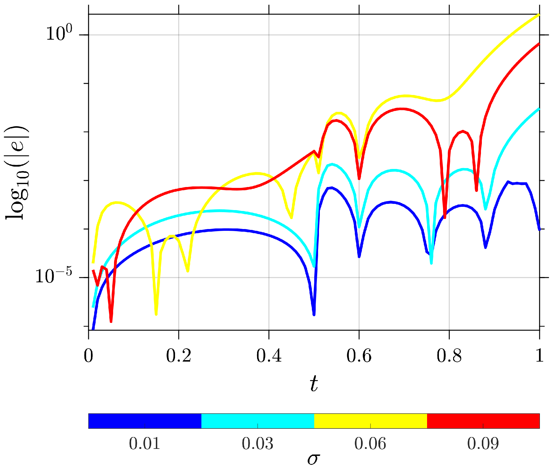
6. Numerical Examples

This section describes the proposed methodology for solving stochastic fractional delay differential equations (SFNDEs) with time-varying delay, as described in Equations (10) and (11), is evaluated. The approach involves considering $\mathbf{Bm}$-discretized Brownian paths and calculating the numerical approximation of $u\left(t\right)$ along these paths. To assess the accuracy of the method, the error concerning the $\mathbf{L}\infty$-norm is employed, defined as

$${\parallel \mathcal{E}n\parallel }_{\infty }=\underset{t\in [0,\mathtt{T}]}{max}\mathbb{E}\left|u\left(t\right)-u_n\left(t\right)\right|,$$

where $u\left(t\right)$ represents the exact solution, and $u_n\left(t\right)$ denotes the numerical approximation. For numerical experiments, Matlab (version 19a) running on an Intel(R) Core(TM) i7-7500U CPU @ 2.70 GHz with a maximum clock speed of 2.90 GHz was used.

Example 1.

Consider the following SFNDE:

$$\begin{array}{cc}\hfill {}^{\mathrm{C}}\mathcal{D}_t^{\eta }[u\left(t\right)-u^2(t-\alpha \left(t\right))]& ={\mathit{e}}^{-u\left(t\right)}u(t-\alpha \left(t\right))+\sigma sin\left(u\left(t\right)\right)u(t-\alpha \left(t\right)){\dot{\mathcal{B}}}_t+f\left(t\right),\hfill \\ \hfill u\left(t\right)& =-t,\mathrm{for}t\in [-\tau ,0],\hfill \end{array}$$

where ${}^{\mathrm{C}}\mathcal{D}_t^{\eta }[·]$ denotes the Caputo fractional derivative of order η, $\sigma \in {\mathbb{R}}^{+}$ is a constant, $\alpha \left(t\right)={\displaystyle \frac{1}{2}}sin\left(\pi t\right)$ represents the time-varying delay, and ${\dot{\mathcal{B}}}_t$ is the formal derivative of the standard Brownian motion.

The piecewise function gives the closed-form solution

$$u\left(t\right)=\left\{\begin{array}{cc}-t,\hfill & t\in [-\tau ,0],\hfill \\ 2t^3,\hfill & t\in (0,\mathtt{T}],\hfill \end{array}\right.$$

where $f\left(t\right)$ is the appropriately chosen source term to satisfy this solution.

Figure 1 presents the solution obtained using the proposed numerical scheme for the SFNDE described in Example 1, alongside its exact solution for parameters $\eta =0.5$, $n=5$, $\sigma =0.01$, $\overline{\mathrm{M}}=20$, $\overline{\mathrm{P}}=45$, $\mathbf{Bm}=250$, and $\mu =0.3$.

Figure 1. The light blue line represents the numerical solution, while the black line shows the exact solution without noise for Example 1 with the parameters $\eta =0.5$, $n=5$, $\sigma =0.01$, $\overline{\mathrm{M}}=20$, $\overline{\mathrm{P}}=45$, $\mathbf{Bm}=250$, and $\mu =0.3$.

In addition, Figure 2 presents a logarithmic analysis of the absolute errors ${log}_{10}|u\left(t\right)-u_n\left(t\right)|$ for the solution of the SFNDE in Example 1 plotted against varying noise intensities $\sigma$. The numerical scheme was implemented with the following parameters: discretization level $n=6$, quadrature orders $\overline{\mathrm{M}}=15$ and $\overline{\mathrm{P}}=45$, fractional order $\eta =0.65$, time step $\mu =0.1$, and $\mathbf{Bm}=200$ Brownian motion realizations. This semi-log plot elucidates the sensitivity of the numerical approximation to stochastic perturbations of different magnitudes. The divergence of error curves for distinct $\sigma$ values provides insight into the method’s stability and accuracy across a spectrum of noise intensities. This analysis is crucial for assessing the robustness and applicability of our numerical scheme in various stochastic environments, particularly when dealing with fractional-order systems subject to time-varying delays and nonlinear interactions. These results provide strong empirical evidence for the efficacy of our proposed method in approximating solutions to SFNDEs with time-varying delays, even in the presence of nonlinear terms and stochastic perturbations.

Figure 2. Logarithmic error analysis, ${log}_{10}\left|e\left(t\right)\right|$, i.e., $e\left(t\right)=u\left(t\right)-u_n\left(t\right)$, in Example 1, illustrating the relationship between the error and noise intensity $\sigma$ for a fractional order of $\eta =0.65$.

Table 1 provides a detailed analysis of computational efficiency and accuracy for Example 1. It includes ${\mathbf{L}}_{\infty }$-norm error values and the CPU time required for various discretization levels (n) with parameters $\eta =0.65$, $\sigma =0.01$, $\overline{\mathrm{P}}=25$, $\overline{\mathrm{M}}=30$, $\mathtt{T}=1$, and $\mathbf{Bm}=200$. The table compares errors for two values of $\mu$ (0.1 and 0.2) and lists the CPU time in seconds.

Table 1. Analysis of computational efficiency and accuracy for the numerical solution in Example 1, highlighting the performance of the proposed method.

Discretization	${\mathit{L}}_{\mathit{\infty }}-\mathbf{Norm}\mathbf{Error}$	${\mathit{L}}_{\mathit{\infty }}-\mathbf{Norm}\mathbf{Error}$	CPU Time
Level n	($\mathit{\mu }=\mathbf{0.1}$)	($\mathit{\mu }=\mathbf{0.2}$)	(seconds)
3	$3.3261\times {10}^{-1}$	$7.1240\times {10}^{-1}$	78.126
6	$5.8410\times {10}^{-2}$	$8.0124\times {10}^{-2}$	141.11
9	$7.1225\times {10}^{-3}$	$3.2636\times {10}^{-2}$	238.812

Example 2.

Consider the SFDDE

$$\begin{array}{cc}\hfill {}^c\mathcal{D}_t^{\eta }[u\left(t\right)+u(t-\alpha \left(t\right))]& =u\left(t\right)u(t-\alpha \left(t\right))+\sigma u^2(t-\alpha \left(t\right)){\dot{\mathcal{B}}}_t+f\left(t\right),\hfill \\ \hfill u\left(t\right)& =0,\mathit{for}t\in [-\tau ,0],\hfill \end{array}$$

where ${}^c\mathcal{D}_t^{\eta }[·]$ denotes the Caputo fractional derivative of order η, $\sigma \in {\mathbb{R}}^{+}$ is the noise intensity, $\alpha \left(t\right)=0.5$ is a constant delay, and ${\dot{\mathcal{B}}}_t$ represents the formal derivative of the standard Brownian motion. The piecewise function gives the analytical solution

$$u\left(t\right)=\left\{\begin{array}{cc}0,\hfill & t\in [-\tau ,0],\hfill \\ tsin\left(\pi t\right),\hfill & t\in (0,\mathtt{T}],\hfill \end{array}\right.$$

where $f\left(t\right)$ is the appropriately chosen source term to satisfy this solution.

Figure 3 presents a comparison between the exact solution and the numerical approximation of Example 2 for $\mathbf{Bm}=300$ Brownian motion realizations and parameters $\eta =0.5$, $n=9$, $\sigma =0.01$, $\overline{\mathrm{P}}=30$, $\overline{\mathrm{M}}=20$, and $\mu =0.2$. In addition, the logarithmic absolute errors ${log}_{10}|u\left(t\right)-u_n\left(t\right)|$ for various values of $\mathbf{Bm}=\{2000,300,400\}$ are shown in Figure 4.

Figure 3. Comparison between the exact solution (black line) and the numerical approximation (light blue line) for Example 2, obtained using the proposed method.

Figure 4. Logarithmic error analysis, ${log}_{10}\left|e\left(t\right)\right|$, i.e., $e\left(t\right)=u\left(t\right)-u_n\left(t\right)$, for Example 2, showing the effect of different numbers of Brownian motion realizations $\mathbf{Bm}$ with a fractional order of $\eta =0.5$.

Table 2 presents the computational efficiency and accuracy of our numerical scheme, displaying the ${\mathbf{L}}_{\infty }$-norm error $\parallel {\mathcal{E}}_n{\parallel }_{\infty }={max}_{t\in [0,\mathtt{T}]}|u\left(t\right)-u_n\left(t\right)|$ and CPU time for varying discretization levels n and time steps $\mu$. The parameters for this analysis are fractional order $\eta =0.45$, noise intensity $\sigma =0.005$, quadrature orders $\overline{\mathrm{P}}=30$ and $\overline{\mathrm{M}}=20$, final time $\mathtt{T}=1$, and $\mathbf{Bm}=250$ Brownian motion realizations.

Table 2. Analysis of computational efficiency and accuracy for the numerical solution in Example 2, demonstrating the performance and reliability of the proposed method.

Discretization	${\mathit{L}}_{\mathit{\infty }}-\mathbf{Norm}\mathbf{Error}$	${\mathit{L}}_{\mathit{\infty }}-\mathbf{Norm}\mathbf{Error}$	CPU Time
Level n	($\mathit{\mu }=\mathbf{0.1}$)	($\mathit{\mu }=\mathbf{0.2}$)	(Seconds)
3	$4.4310\times {10}^{-2}$	$7.5463\times {10}^{-1}$	$42.24$
6	$3.2467\times {10}^{-3}$	$5.4505\times {10}^{-2}$	$73.108$
9	$4.3311\times {10}^{-4}$	$2.1173\times {10}^{-2}$	$164.34$

This thorough analysis highlights the proposed numerical scheme’s accuracy, stability, and computational efficiency when solving SFDDEs with constant delays. It provides valuable insights into the scheme’s performance across different parameter configurations and stochastic realizations.

Example 3.

A comprehensive population growth model for E. coli that demonstrates a prolonged, step-like growth pattern is proposed by NDDE [47]. The proposed model encompasses the following critical features: (i) all cells exhibit identical division times, (ii) cellular division occurs synchronously, (iii) there is an initial period characterized by extended step-like growth, and (iv) the initial population size of E. coli colonies remains indeterminate. That is

$${}^c\mathcal{D}_t^{\eta }[u\left(t\right)-{\rho }_{2}u(t-\tau )]={\rho }_{0}u\left(t\right)+{\rho }_{1}u(t-\tau )+\sigma {\dot{\mathcal{B}}}_t,\eta \in (0,1],$$

(52)

where $u\left(t\right)$ represents the population, and the history function is given by

$$\varphi \left(t\right)=u_0+\beta \Psi \left(t\right),t\in [-\tau ,0],$$

where

$$\Psi \left(t\right)={\displaystyle \frac{2u_0\beta \gamma }{{\rho }_1\tau }}E\left({\displaystyle \frac{2t}{h}}+1\right),$$

and

$$E\left(t\right)=\left\{\begin{array}{cc}exp\left(-{\displaystyle \frac{1}{1-t^2}}\right),\hfill & \mathit{for}\left|t\right|<1,\hfill \\ 0,\hfill & \mathit{otherwise}.\hfill \end{array}\right.$$

where ${\rho }_0=0.004$ is the growth rate parameter, ${\rho }_1=0.004$ is the interaction effect parameter, ${\rho }_2=0.101$ is the delay effect parameter, $\tau =1.623$ is the delay time in hours, $u_0=99$ is the initial population of E. coli cells, $\beta =0.011$ is a scaling factor, $\gamma =2.25$ is the growth efficiency, and $h=1$ is the characteristic time scale. These values are typical and derived from empirical observations in microbial growth studies, providing a solid foundation for modeling E. coli population dynamics.

Figure 5 illustrates the simulation results for various values of $\eta$ with the numerical algorithm parameters set as $n=21$, $\sigma =0.01$, $\overline{\mathrm{P}}=80$, $\overline{\mathrm{M}}=2n+1$, and $\mu =0.5$. The black line corresponds to the integer-order solution based on the approach from [48], showing strong agreement with the proposed model at $\eta =1$. Moreover, the obtained numerical solutions leverage the Martingale property of the stochastic process, implying that while the solution exhibits random fluctuations, it shows no deterministic trend or drift. Although these fluctuations are more pronounced in the integer-order solution obtained using the approach from [48], they are less visible in the proposed method due to the use of a low-degree interpolating polynomial, which leads to a natural averaging effect. Additionally, as the fractional order decreases, an exponential decline in the growth rate is observed, consistent with the theoretical expectations for such systems.

Figure 5. Simulation results of the E. coli population growth model for various values of $\eta$, and with the parameters set as $n=21$, $\sigma =0.01$, $\overline{\mathrm{P}}=80$, $\overline{\mathrm{M}}=2n+1$, and $\mu =0.5$. The black line represents the integer-order solution obtained by the method proposed in [48].

7. Conclusions

This study presented a novel numerical approach for solving fractional neutral stochastic differential equations (SFDDEs) with a neutral delay. The method leveraged Jacobi poly-fractonomials to transform the original problem into a non-delay stochastic neutral integral equation. By applying a collocation scheme based on these poly-fractonomials, the non-delay equations were reduced to systems of nonlinear algebraic equations, which were solved iteratively. The convergence analysis demonstrated that the proposed method exhibits spectral convergence, highlighting its efficiency and accuracy. Numerical examples further validated the robustness and effectiveness of the approach, showing its capability to handle the complexities of SFDDEs with high precision.

Since the fractional operator used in this study is not memoryless and is constrained by the lower terminal of the fractional operator, the need for higher-degree polynomials for extended solution times is inevitable. As the polynomial degree increases, the number of unknowns in the nonlinear augmented algebraic equations also grows, potentially leading to an exponential increase in computation time. This issue could be addressed by using short-memory memory principal [49]. Future work will focus on investigating this approach further.

References

- Dobrushkin, V.A. Applied Differential Equations with Boundary Value Problems; Chapman and Hall/CRC: New York, NY, USA, 2017. [Google Scholar] [CrossRef]
- Nandakumaran, A.; Datti, P.; George, R. Ordinary Differential Equations: Principles and Applications; Cambridge IISc Series; Cambridge University Press: Cambridge, UK, 2017. [Google Scholar]
- Nilsson, J.; Riedel, S. Electric Circuits; Pearson Education: London, UK, 2014. [Google Scholar]
- Chopra, A. Dynamics of Structures: Theory and Applications to Earthquake Engineering; Pearson Education: London, UK; Prentice Hall: Upper Saddle River, NJ, USA, 2000. [Google Scholar]
- Oksendal, B. Stochastic Differential Equations, An Introduction with Applications; Springer: New York, NY, USA, 1998. [Google Scholar]
- Chen, X.; Hu, P.; Shum, S.; Zhang, Y. Dynamic stochastic inventory management with reference price effects. Oper. Res. 2016, 64, 1529–1536. [Google Scholar] [CrossRef]
- Huu, A.; Costa-Lima, B. Orbits in a stochastic Goodwin-Lotka-Volterra model. J. Math. Anal. Appl. 2014, 419, 48–67. [Google Scholar]
- Ahmadi, Z.; Mohammad Hosseini, S.; Foroush Bastani, A. A lattice-based approach to option and bond valuation under mean-reverting regime-switching diffusion processes. J. Comput. Appl. Math. 2020, 363, 156–170. [Google Scholar] [CrossRef]
- Bellomo, N.; Brzezniak, Z.; de Socio, L. Nonlinear Stochastic Evolution Problems in Applied Sciences; Kluwer Academic Publishers/Springer: Dordrecht, The Netherlands, 1992. [Google Scholar]
- Qi, J.; Cui, Q.; Bai, L.; Sun, Y. Investigating exact solutions, sensitivity, and chaotic behavior of multi-fractional order stochastic Davey-Sewartson equations for hydrodynamics research applications. Chaos Solitons Fractals 2024, 180, 114491. [Google Scholar] [CrossRef]
- Singh, S.; Ray, S. Numerical solutions of stochastic Fisher equation to study migration and population behavior in biological invasion. Int. J. Biomath. 2017, 10, 1750103. [Google Scholar] [CrossRef]
- Padgett, W.; Tsokos, C. A new stochastic formulation of a population growth problem. Math. Biosci. 1973, 17, 105–120. [Google Scholar] [CrossRef]
- Aboulaich, R.; Darouichi, A.; Elmouki, I.; Jraifi, A. A Stochastic Optimal Control Model for BCG Immunotherapy in Superficial Bladder Cancer. Math. Model. Nat. Phenom. 2017, 12, 99–119. [Google Scholar] [CrossRef]
- Yang, J.; Tan, Y.; Cheke, R. Thresholds for extinction and proliferation in a stochastic tumour-immune model with pulsed comprehensive therapy. Commun. Nonlinear Sci. Numer. Simulat. 2019, 73, 363–378. [Google Scholar] [CrossRef]
- Jerez, S.; Diaz-Infante, S.; Chen, B. Fluctuating periodic solutions and moment boundedness of a stochastic model for the bone remodeling process. Math. Biosci. 2018, 299, 153–164. [Google Scholar] [CrossRef]
- Babaei, A.; Jafari, H.; Banihashemi, S.; Ahmadi, M. Mathematical analysis of a stochastic model for spread of Coronavirus. Chaos Solitons Fractals 2021, 145, 110788. [Google Scholar] [CrossRef]
- Dabiri, A.; Butcher, E.A.; Poursina, M.; Nazari, M. Optimal periodic-gain fractional delayed state feedback control for linear fractional periodic time-delayed systems. IEEE Trans. Autom. Control. 2017, 63, 989–1002. [Google Scholar] [CrossRef]
- Balachandran, B.; Kalmár-Nagy, T.; Gilsinn, D.E. Delay Differential Equations; Springer: New York, NY, USA, 2009. [Google Scholar]
- Forde, J.E. Delay Differential Equation Models in Mathematical Biology; University of Michigan: Ann Arbor, MI, USA, 2005. [Google Scholar]
- Erneux, T. Applied Delay Differential Equations; Springer: New York, NY, USA, 2009. [Google Scholar]
- Karimi, R.; Dabiri, A.; Cheng, J.; Butcher, E.A. Probabilistic-robust optimal control for uncertain linear time-delay systems by state feedback controllers with memory. In Proceedings of the 2018 Annual American Control Conference (ACC), Wisconsin, MI, USA, 27–29 June 2018; pp. 4183–4188. [Google Scholar]
- Podlubny, I. Fractional Differential Equations: An Introduction to Fractional Derivatives, Fractional Differential Equations, to Methods of Their Solution and Some of Their Applications; Academic Press: San Diego, CA, USA; London, UK, 1998. [Google Scholar]
- Parsa Moghaddam, B.; Dabiri, A.; Mostaghim, Z.S.; Moniri, Z. Numerical solution of fractional dynamical systems with impulsive effects. Int. J. Mod. Phys. C 2023, 34, 2350013. [Google Scholar] [CrossRef]
- Dabiri, A.; Butcher, E.A.; Nazari, M. Coefficient of restitution in fractional viscoelastic compliant impacts using fractional Chebyshev collocation. J. Sound Vib. 2017, 388, 230–244. [Google Scholar] [CrossRef]
- Moghaddam, B.P.; Dabiri, A.; Machado, J.A.T. Application of variable-order fractional calculus in solid mechanics. In Volume 7 Applications in Engineering, Life and Social Sciences, Part A; De Gruyter: Berlin, Germany, 2019. [Google Scholar]
- Dabiri, A.; Moghaddam, B.; Machado, J.T. Optimal variable-order fractional PID controllers for dynamical systems. J. Comput. Appl. Math. 2018, 339, 40–48. [Google Scholar] [CrossRef]
- Moniri, Z.; Parsa Moghaddam, B.; Zamani Roudbaraki, M. An Efficient and Robust Numerical Solver for Impulsive Control of Fractional Chaotic Systems. Math. Probl. Eng. 2023, 2023, 9077924. [Google Scholar] [CrossRef]
- Ionescu, C.; Lopes, A.; Copot, D.; Machado, J.T.; Bates, J.H. The role of fractional calculus in modeling biological phenomena: A review. Commun. Nonlinear Sci. Numer. Simul. 2017, 51, 141–159. [Google Scholar] [CrossRef]
- Baleanu, D. Fractional Calculus: Models and Numerical Methods; World Scientific: Singapore, 2012; Volume 3. [Google Scholar]
- Moghaddam, B.P.; Zhang, L.; Lopes, A.M.; Tenreiro Machado, J.A.; Mostaghim, Z.S. Sufficient conditions for existence and uniqueness of fractional stochastic delay differential equations. Int. J. Probab. Stoch. Process. 2019, 92, 379–396. [Google Scholar] [CrossRef]
- Ayazi, N.; Mokhtary, P.; Moghaddam, B.P. Efficiently solving fractional delay differential equations of variable order via an adjusted spectral element approach. Chaos Solitons Fractals 2024, 181, 114635. [Google Scholar] [CrossRef]
- Banihashemi, S.; Jafari, H.; Babaei, A. A novel collocation approach to solve a nonlinear stochastic differential equation of fractional order involving a constant delay. Discret. Contin. Dyn. Syst. Ser. S 2021, 15, 339–357. [Google Scholar] [CrossRef]
- Moghaddam, B.P.; Pishbin, M.; Mostaghim, Z.S.; Iyiola, O.S.; Galhano, A.; Lopes, A.M. A Numerical Algorithm for Solving Nonlocal Nonlinear Stochastic Delayed Systems with Variable-Order Fractional Brownian Noise. Fractal Fract. 2023, 7, 293. [Google Scholar] [CrossRef]
- Chadha, A.; Pandey, D.; Bahuguna, D. Faedo–Galerkin approximate solutions of a neutral stochastic fractional differential equation with finite delay. J. Comput. Appl. Math. 2018, 347, 238–256. [Google Scholar] [CrossRef]
- Chaudhary, R.; Pandey, D.N. Approximation of Solutions to Stochastic Neutral Fractional Integro-Differential Equation with Nonlocal Conditions. Int. J. Appl. Comput. Math. 2017, 3, 1203–1223. [Google Scholar] [CrossRef]
- Rahimkhani, P.; Ordokhani, Y. Chelyshkov least squares support vector regression for nonlinear stochastic differential equations by variable fractional Brownian motion. Chaos Solitons Fractals 2022, 163, 112570. [Google Scholar] [CrossRef]
- Dabiri, A.; Butcher, E.A. Numerical solution of multi-order fractional differential equations with multiple delays via spectral collocation methods. Appl. Math. Model. 2018, 56, 424–448. [Google Scholar] [CrossRef]
- Dabiri, A.; Butcher, E.A. Efficient modified Chebyshev differentiation matrices for fractional differential equations. Commun. Nonlinear Sci. Numer. Simul. 2017, 50, 284–310. [Google Scholar] [CrossRef]
- Kazem, S. An integral operational matrix based on Jacobi polynomials for solving fractional-order differential equations. Appl. Math. Model. 2013, 37, 1126–1136. [Google Scholar] [CrossRef]
- Dastgerdi, M.V.; Bastani, A.F. Solving Parametric Fractional Differential Equations Arising from the Rough Heston Model Using Quasi-Linearization and Spectral Collocation. SIAM J. Financ. Math. 2020, 11, 1063–1097. [Google Scholar] [CrossRef]
- Zayernouri, M.; Karniadakis, G.E. Exponentially accurate spectral and spectral element methods for fractional ODEs. J. Comput. Phys. 2014, 257, 460–480. [Google Scholar] [CrossRef]
- Duan, B.; Zheng, Z.; Cao, W. Spectral approximation methods and error estimates for Caputo fractional derivative with applications to initial-value problems. J. Comput. Phys. 2016, 319, 108–128. [Google Scholar] [CrossRef]
- Hussaini, M.Y.; Zang, T.A. Spectral Methods in Fluid Dynamics; Technical report; Springer: Berlin/Heidelberg, Germany, 1986. [Google Scholar]
- Choe, G. Stochastic Analysis for Finance with Simulations; Springer: Cham, Switzerland, 2016. [Google Scholar]
- Aryani, E.; Babaei, A.; Valinejad, A. A numerical technique for solving nonlinear fractional stochastic integro-differential equations with n-dimensional Wiener process. Comput. Methods Differ. Equ. 2021, 10, 61–76. [Google Scholar] [CrossRef]
- Kamrani, M. Numerical solution of stochastic fractional differential equations. Numer. Algorithms 2015, 68, 81–93. [Google Scholar] [CrossRef]
- Jamilla, C.U.; Mendoza, R.G.; Mendoza, V.M.P. Parameter Estimation in Neutral Delay Differential Equations Using Genetic Algorithm With Multi-Parent Crossover. IEEE Access 2021, 9, 131348–131364. [Google Scholar] [CrossRef]
- Shampine, L.F. Dissipative approximations to neutral DDEs. Appl. Math. Comput. 2008, 203, 641–648. [Google Scholar] [CrossRef]
- Deng, W. Short memory principle and a predictor–corrector approach for fractional differential equations. J. Comput. Appl. Math. 2007, 206, 174–188. [Google Scholar] [CrossRef]
Disclaimer/Publisher’s Note: The statements, opinions and data contained in all publications are solely those of the individual author(s) and contributor(s) and not of MDPI and/or the editor(s). MDPI and/or the editor(s) disclaim responsibility for any injury to people or property resulting from any ideas, methods, instructions or products referred to in the content. |
© 2024 by the authors. Licensee MDPI, Basel, Switzerland. This article is an open access article distributed under the terms and conditions of the Creative Commons Attribution (CC BY) license (https://creativecommons.org/licenses/by/4.0/).