
Robust Classification via Finite Mixtures of Matrix Variate Skew-t Distributions


Abstract
1. Introduction
2. Related Studies
3. Methodology
3.1. The Model
3.2. Parameter Estimation via the ECME Algorithm
- CMQ step 1: Fixing , we update by maximizing (24) with respect to , leading to
- CMQ step 2: Fixing , and , we then update by maximizing (24) over , yielding
- CMQ step 3: Fixing , and , we update by maximizing (24) over , yielding
- CMQ step 4: Fixing , we obtain by maximizing (24) over , yielding
- CML step: Update by optimizing the following constrained log likelihood function:
4. Fitting Finite Mixtures of MVST Distributions
4.1. The Model
- E step: Given , compute , , and given in (27), for and ;
- CM step 1: Calculate
- CM step 2: Update as
- CM step 3: Update as
- CM step 4: Update as
- CM step 5: Update as
- CML step: Update by optimizing the constrained log likelihood function as
4.2. Initialization
4.3. Identifiability
5. Empirical Study
5.1. Finite-Sample Properties of ML Estimators
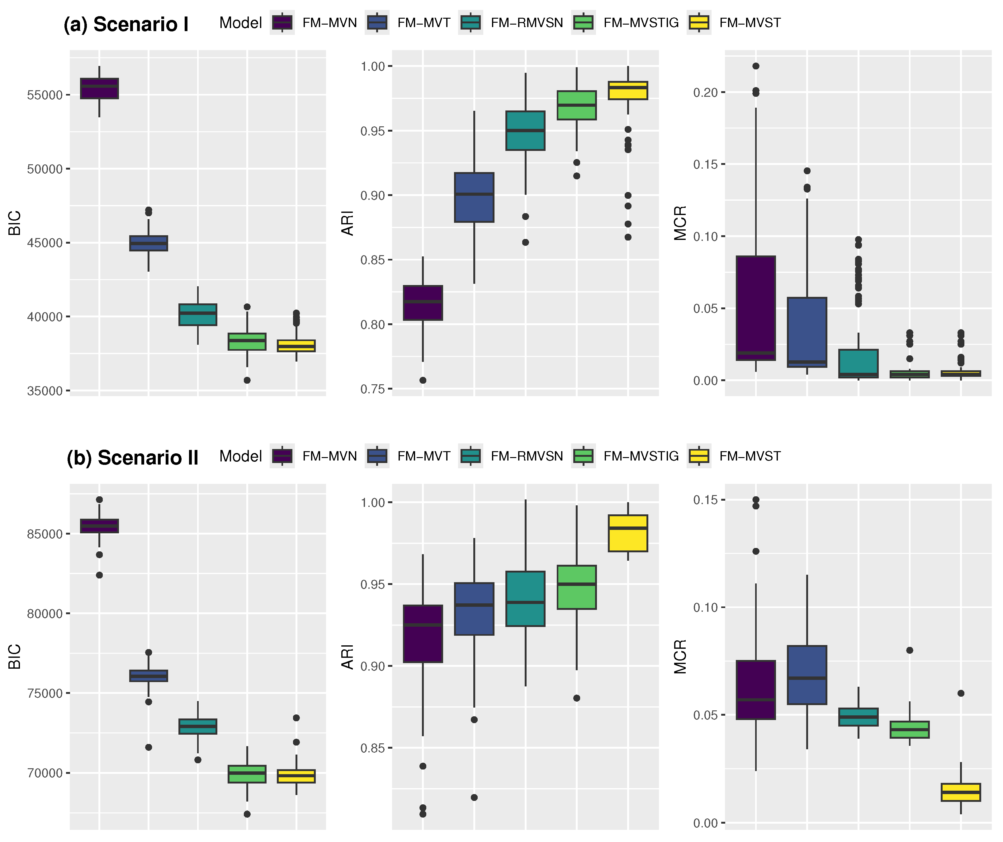
5.2. Comparison of Classification Accuracy
6. Real Data Analysis
6.1. Landsat Data
6.2. Apes Data
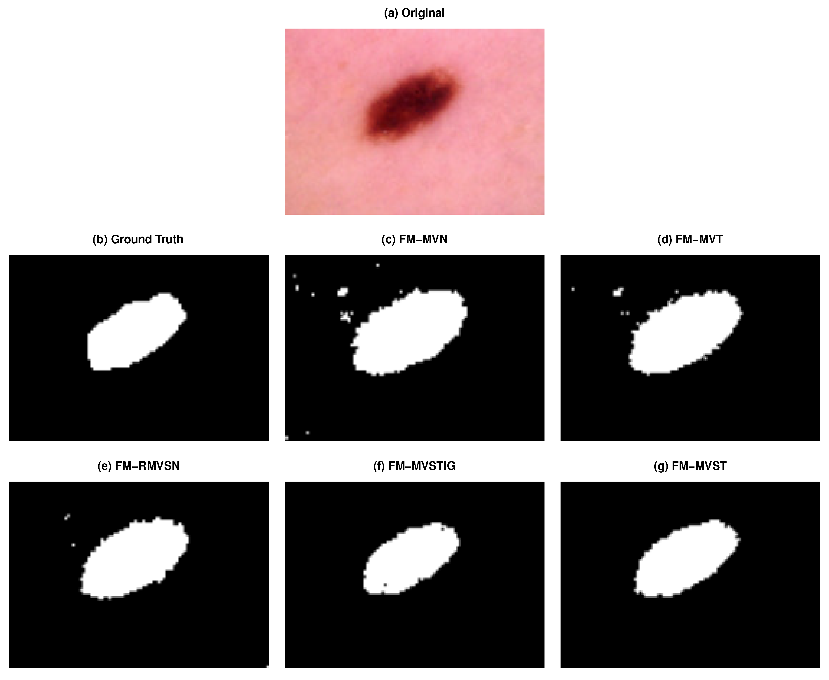
6.3. Melanoma Data
7. Concluding Remarks
Author Contributions
Funding
Data Availability Statement
Conflicts of Interest
Appendix A

| Scenario | Parameter | Component 1 | Component 2 |
|---|---|---|---|
| I | 0.3 | 0.7 | |
| 3 | 5 | ||
| II | 0.4 | 0.6 | |
| 4 | 4 |
References
- Kroonenberg, P.M. Applied Multiway Data Analysis; John Wiley & Sons: Hoboken, NJ, USA, 2008. [Google Scholar]
- Dickey, J.M. Matricvariate generalizations of the multivariate t distribution and the inverted multivariate t distribution. Ann. Math. Stat. 1967, 38, 511–518. [Google Scholar] [CrossRef]
- Arellano-Valle, R.B.; Azzalini, A. A formulation for continuous mixtures of multivariate normal distributions. J. Multivar. Anal. 2021, 185, 104780. [Google Scholar] [CrossRef]
- Liu, C.; Rubin, D.B. The ECME algorithm: A simple extension of EM and ECM with faster monotone convergence. Biometrika 1994, 81, 633–648. [Google Scholar] [CrossRef]
- Dempster, A.P.; Laird, N.M.; Rubin, D.B. Maximum likelihood from incomplete data via the EM algorithm. J. R. Stat. Soc. Ser. (Methodol.) 1977, 39, 1–22. [Google Scholar] [CrossRef]
- Rezaei, A.; Yousefzadeh, F.; Arellano-Valle, R.B. Scale and shape mixtures of matrix variate extended skew normal distributions. J. Multivar. Anal. 2020, 179, 104649. [Google Scholar] [CrossRef]
- Gallaugher, M.P.; McNicholas, P.D. A matrix variate skew-t distribution. Stat 2017, 6, 160–170. [Google Scholar] [CrossRef]
- Gallaugher, M.P.; McNicholas, P.D. Finite mixtures of skewed matrix variate distributions. Pattern Recognit. 2018, 80, 83–93. [Google Scholar] [CrossRef]
- Naderi, M.; Bekker, A.; Arashi, M.; Jamalizadeh, A. A theoretical framework for Landsat data modeling based on the matrix variate mean-mixture of normal model. PLoS ONE 2020, 15, e0230773. [Google Scholar] [CrossRef]
- Chen, J.T.; Gupta, A.K. Matrix variate skew normal distributions. Statistics 2005, 39, 247–253. [Google Scholar] [CrossRef]
- Domínguez-Molina, J.A.; González-Farías, G.; Ramos-Quiroga, R.; Gupta, A.K. A matrix variate closed skew-normal distribution with applications to stochastic frontier analysis. Commun. Stat.—Theory Methods 2007, 36, 1691–1703. [Google Scholar] [CrossRef]
- Zhang, L.; Bandyopadhyay, D. A graphical model for skewed matrix-variate non-randomly missing data. Biostatistics 2020, 21, e80–e97. [Google Scholar] [CrossRef]
- Viroli, C. Finite mixtures of matrix normal distributions for classifying three-way data. Stat. Comput. 2011, 21, 511–522. [Google Scholar] [CrossRef]
- Thompson, G.Z.; Maitra, R.; Meeker, W.Q.; Bastawros, A.F. Classification with the matrix-variate-t distribution. J. Comput. Graph. Stat. 2020, 29, 668–674. [Google Scholar] [CrossRef]
- Tomarchio, S.D.; Punzo, A.; Bagnato, L. Two new matrix-variate distributions with application in model-based clustering. Comput. Stat. Data Anal. 2020, 152, 107050. [Google Scholar] [CrossRef]
- Tomarchio, S.D.; Gallaugher, M.P.; Punzo, A.; McNicholas, P.D. Mixtures of matrix-variate contaminated normal distributions. J. Comput. Graph. Stat. 2022, 31, 413–421. [Google Scholar] [CrossRef]
- Tomarchio, S.D. Matrix-variate normal mean-variance Birnbaum–Saunders distributions and related mixture models. Comput. Stat. 2024, 39, 405–432. [Google Scholar] [CrossRef]
- Naderi, M.; Tamandi, M.; Mirfarah, E.; Wang, W.L.; Lin, T.I. Three-way data clustering based on the mean-mixture of matrix-variate normal distributions. Comput. Stat. Data Anal. 2024, 199, 108016. [Google Scholar] [CrossRef]
- Lin, T.I.; Wu, P.H.; McLachlan, G.J.; Lee, S.X. A robust factor analysis model using the restricted skew-t distribution. Test 2015, 24, 510–531. [Google Scholar] [CrossRef]
- Lee, S.X.; McLachlan, G.J. Finite mixtures of canonical fundamental skew t-distributions: The unification of the restricted and unrestricted skew t-mixture models. Stat. Comput. 2016, 26, 573–589. [Google Scholar] [CrossRef]
- Macqueen, J. Some methods for classification and analysis of multivariate observations. In Proceedings of the 5th Berkeley Symposium on Mathematical Statistics and Probability, Davis, CA, USA, 21 June–18 July 1965; University of California Press: Berkeley, CA, USA, 1967. [Google Scholar]
- Lloyd, S. Least squares quantization in PCM. IEEE Trans. Inf. Theory 1982, 28, 129–137. [Google Scholar] [CrossRef]
- Sarkar, S.; Zhu, X.; Melnykov, V.; Ingrassia, S. On parsimonious models for modeling matrix data. Comput. Stat. Data Anal. 2020, 142, 106822. [Google Scholar] [CrossRef]
- Hubert, L.; Arabie, P. Comparing partitions. J. Classif. 1985, 2, 193–218. [Google Scholar] [CrossRef]
- Schwarz, G. Estimating the dimension of a model. Ann. Stat. 1978, 461–464. [Google Scholar] [CrossRef]
- Dryden, I.L. shapes Package; Version 1.2.6; Contributed package; R Foundation for Statistical Computing: Vienna, Austria, 2021. [Google Scholar]
- Dryden, I.; Mardia, K. Statistical Shape Analysis: With Applications in R; Wiley Series in Probability and Statistics; Wiley: Hoboken, NJ, USA, 2016. [Google Scholar]
| Scenario | N | |||||||||||
|---|---|---|---|---|---|---|---|---|---|---|---|---|
| I | 250 | 0.031 | 0.169 | 0.119 | 0.058 | 0.045 | 0.128 | 0.078 | 0.174 | 0.118 | 1.638 | 3.629 |
| 500 | 0.020 | 0.129 | 0.087 | 0.044 | 0.041 | 0.093 | 0.064 | 0.126 | 0.088 | 1.215 | 3.128 | |
| 1000 | 0.015 | 0.091 | 0.059 | 0.032 | 0.031 | 0.066 | 0.052 | 0.088 | 0.056 | 0.803 | 2.712 | |
| 2000 | 0.011 | 0.062 | 0.044 | 0.027 | 0.028 | 0.051 | 0.043 | 0.062 | 0.044 | 0.702 | 2.230 | |
| II | 250 | 0.035 | 0.260 | 0.193 | 1.348 | 0.376 | 0.785 | 0.440 | 0.257 | 0.187 | 2.544 | 2.426 |
| 500 | 0.022 | 0.176 | 0.130 | 1.257 | 0.338 | 0.771 | 0.425 | 0.179 | 0.129 | 2.297 | 2.219 | |
| 1000 | 0.014 | 0.120 | 0.097 | 1.206 | 0.312 | 0.764 | 0.423 | 0.124 | 0.097 | 1.962 | 1.897 | |
| 2000 | 0.011 | 0.088 | 0.068 | 1.184 | 0.302 | 0.753 | 0.401 | 0.090 | 0.070 | 1.460 | 1.388 |
| Scenario | Model | BIC | Std | ARI | Std | MCR | Std |
|---|---|---|---|---|---|---|---|
| FM-MVN | 55,419.78 | 831.20 | 0.82 | 0.20 | 0.05 | 0.06 | |
| FM-MVT | 45,004.95 | 787.39 | 0.90 | 0.17 | 0.03 | 0.05 | |
| I | FM-RMVSN | 40,103.90 | 962.33 | 0.95 | 0.18 | 0.02 | 0.05 |
| FM-MVSTIG | 38,215.01 | 859.47 | 0.97 | 0.08 | 0.01 | 0.02 | |
| FM-MVST | 38,170.98 | 804.07 | 0.98 | 0.05 | 0.01 | 0.01 | |
| FM-MVN | 85,450.81 | 705.80 | 0.91 | 0.15 | 0.07 | 0.06 | |
| FM-MVT | 76,011.44 | 720.48 | 0.93 | 0.14 | 0.08 | 0.05 | |
| II | FM-RMVSN | 72,917.04 | 703.48 | 0.94 | 0.12 | 0.05 | 0.02 |
| FM-MVSTIG | 69,892.52 | 694.08 | 0.95 | 0.10 | 0.04 | 0.02 | |
| FM-MVST | 69,839.90 | 673.31 | 0.97 | 0.09 | 0.02 | 0.01 |
| Model | G | Log Likelihood | BIC | ARI | MCR |
|---|---|---|---|---|---|
| FM-MVN | −114,954.90 | 231,799.40 | 0.67 | 0.14 | |
| FM-MVT | −113,169.30 | 228,228.10 | 0.69 | 0.13 | |
| FM-RMVSN | 3 | −111,213.50 | 225,107.40 | 0.76 | 0.09 |
| FM-MVSTIG | −110,920.90 | 224,543.20 | 0.79 | 0.07 | |
| FM-MVST | −110,836.60 | 224,374.60 | 0.82 | 0.06 |
| Model | G | Log Likelihood | BIC | ARI | MCR |
|---|---|---|---|---|---|
| FM-MVN | −7773.14 | 17,204.51 | 0.51 | 0.41 | |
| FM-MVT | −7609.66 | 16,877.54 | 0.56 | 0.32 | |
| FM-RMVSN | 6 | −6158.09 | 14,522.03 | 0.60 | 0.28 |
| FM-MVSTIG | −6097.66 | 14,431.87 | 0.63 | 0.27 | |
| FM-MVST | −5970.42 | 14,177.41 | 0.67 | 0.25 |
| Model | G | Log Likelihood | BIC | ARI | MCR |
|---|---|---|---|---|---|
| FM-MVN | 63,941.64 | −127,723.90 | 0.76 | 0.14 | |
| FM-MVT | 65,509.39 | −130,859.40 | 0.82 | 0.13 | |
| FM-RMVSN | 2 | 65,601.15 | −130,945.50 | 0.91 | 0.12 |
| FM-MVSTIG | 65,788.76 | −131,303.10 | 0.93 | 0.11 | |
| FM-MVST | 67,241.98 | −134,209.50 | 0.95 | 0.09 |
Disclaimer/Publisher’s Note: The statements, opinions and data contained in all publications are solely those of the individual author(s) and contributor(s) and not of MDPI and/or the editor(s). MDPI and/or the editor(s) disclaim responsibility for any injury to people or property resulting from any ideas, methods, instructions or products referred to in the content. |
© 2024 by the authors. Licensee MDPI, Basel, Switzerland. This article is an open access article distributed under the terms and conditions of the Creative Commons Attribution (CC BY) license (https://creativecommons.org/licenses/by/4.0/).
Share and Cite
Mahdavi, A.; Balakrishnan, N.; Jamalizadeh, A. Robust Classification via Finite Mixtures of Matrix Variate Skew-t Distributions. Mathematics 2024, 12, 3260. https://doi.org/10.3390/math12203260
Mahdavi A, Balakrishnan N, Jamalizadeh A. Robust Classification via Finite Mixtures of Matrix Variate Skew-t Distributions. Mathematics. 2024; 12(20):3260. https://doi.org/10.3390/math12203260
Chicago/Turabian StyleMahdavi, Abbas, Narayanaswamy Balakrishnan, and Ahad Jamalizadeh. 2024. "Robust Classification via Finite Mixtures of Matrix Variate Skew-t Distributions" Mathematics 12, no. 20: 3260. https://doi.org/10.3390/math12203260
APA StyleMahdavi, A., Balakrishnan, N., & Jamalizadeh, A. (2024). Robust Classification via Finite Mixtures of Matrix Variate Skew-t Distributions. Mathematics, 12(20), 3260. https://doi.org/10.3390/math12203260