Abstract
In this paper, we employed the -dressing method to investigate the Kundu-nonlinear Schrödinger equation based on the local 2 × 2 matrix problem. The Lax spectrum problem is used to derive a singular spectral problem of time and space associated with a Kundu-NLS equation. The N-solitions of the Kundu-NLS equation were obtained based on the equation by choosing a special spectral transformation matrix, and a gradual analysis of the long-duration behavior of the equation was acquired. Subsequently, the one- and two-soliton solutions of Kundu-NLS equations were obtained explicitly. In optical fiber, due to the wide application of telecommunication and flow control routing systems, people are very interested in the propagation of femtosecond optical pulses, and a high-order, nonlinear Schrödinger equation is needed to build a model. In plasma physics, the soliton equation can predict the modulation instability of light waves in different media.
MSC:
35C08; 35Q51; 37K40
1. Introduction
In recent years, the nonlinear Schrödinger equation (NLS) [1,2] has emerged as an important component of the soliton equation. It appears in many different physical applications, such as in plasma physics and nonlinear optics [3], which have a wide range of applications. With the advances of this research, the classical Schrödinger equation [4,5,6],
and its evolutionary form can represent a well-known integrable system in the field of mathematics. In Equation (1), u denotes the complex envelope of the waves, x and t denote propagation distance and scaled time, respectively, and i is the imaginary unit. The Schrödinger equation has a stable soliton solution, which can be properly denoted by the linear dispersion problems. However, in physics, particularly in optical fibers, this model needs to be described using the high-order Schrodinger equation because of interest in the propagation of femtosecond light pulses. In the field of mathematics, the study of nonlinear equations with variable coefficients has also led to the further development of integrable systems. The similar transformation technique, Wronskian technique, Jacobi elliptic approach, and direct algebraic method can solve the nonlinear Schrodinger equation with variable coefficients [7,8,9,10]. By using the similar transformation technique, we can solve the optically smooth position solution of the nonlinear Schrodinger equation with variable coefficients. In 1984, Kundu proved that the nonlinear Schrödinger equation leads to an integrable high-order nonlinear equation with variable coefficients under nonlinear transformation, which is called the Kundu-NLS equation. It can be associated with the nonlinear Schrödinger equation via the Lax equation, and it does not change the dispersion term.
In this article, we focus primarily on the Kundu-NLS equation [11,12,13,14,15,16],
where is a free gauge function, and is a real constant. Using the -dressing method, we created one- and two-soliton solutions. The equation of the respirator and higher-order rouge wave solutions was obtained using the Darboux transform [15,16]. It is also possible to obtain the equation’s soliton solution by using the Riemann–Hilbert method [11,12,13,14]. As far as we know, the soliton solution of the Kundu-NLS equations has not been solved by using the -dressing method.
The -dressing method suggested by Zakharov and Shabat [17,18] was later developed by Beals, Coifman, Manakov, Ablowitz, Fokas, and others [19,20,21,22,23]. A wide variety of equations have been successfully investigated using the -dressing method [24,25,26,27,28,29,30]. However, the equations with a normalization boundary condition, , at infinity are usually considered. Consequently, the spectral problems and hierarchies on some significant integrable equations, such as the KE equation, Kundu-NLS equations, and others, cannot be adequately deduced using the -dressing method. We are primarily concerned with the -equation for normalization, , where D is a nondegenerate matrix function of x and t. Using the -dressing method, the Lax pair and deriving the soliton solutions could be investigated.
The structure of this article is as follows: In Section 2, by using the -dressing method, we obtained the Lax pair by generalizing the properties of the Cauchy–Green operators. In Section 2.2, by using the -dressing method, we derived the Kundu-NLS hierarchy (with the source) from the relationship between the -dressing transformation matrix and the potential matrix. In Section 3, a formula for N-soliton solutions of the Kundu-NLS equation was constructed, and we give explicit one- and two-soliton solutions for the Kundu-NLS equation.
2. The -Dressing Method
2.1. Spectral Transform and Lax Pair
In this section, in order to analyze the Kundu-NLS equation, we focus on the Lax pair of Equation (2):
where , with , .
Consider a matrix problem with a non-normalization boundary condition. The -dressing method’s objective is to create a system of linear equations for that is compatible. We start from the matrix -problem in the complex z-plane,
where is a nondegenerate matrix function of x and t, and is the matrix of spectral transform connected to a nonlinear equation and . We obtained a formal solution of the -problem via Equation (4):
where represents the Cauchy–Green integral operator on the left, and this is given by
In this case, we suppressed the fact that the variable depends on and R. The expression in Equation (5) empowers us to officially compose an answer to the issue (5) concerning the matrix R:
where I is the unit matrix.
Define
where D satisfied , .
It is simple to demonstrate that the operator satisfies (for a certain set of matrix functions) and ,
Define a pair:
where the superscript T means transposition. Then, it is evident that the above pairing has the following features [24].
Proposition 1.
In addition, it will be easy to test and verify the following prosperities:
and
or, in general, for some positive integer ,
where is defined by putting .
We allow the x-dependence of the Kundu-NLS equation to be expressed as follows. It is significant that the form of the Lax pair for a particular equation is entirely determined by the space–time dependence of the transform matrix :
Then, Equation (7) can be utilized to compute
The first term on the right can be transformed as follows:
Hence,
Next, we calculate the second term, , from Equation (17), where we have
As a result,
Next, we introduce the potential:
then we can also obtain the spectral problem of Zakharov–Shabat:
In order to acquire the time dependency of R, we select a linear equation such that
We suppose
which comprises both a polynomial part, , and a singular part, , and is a scalar function.
First, we use the polynomial dispersion relation only, = = . Then, using Equations (5), (7), and (22), we obtain
We form the definition of the left Cauchy operation:
and
We suppose means the off-diagonal part of matrix •, and means the diagonal part of matrix •. Furthermore,
So, the time-spectral problem is obtained:
In what follows, we consider the singular dispersion relation in Equation (23):
Hence, we have
By using the relations
we find that
according to which Equation (36) then gives a time-dependent linear equation with the singular dispersion relation:
The time-spectral problem is
2.2. Recursion Operator
In this section, we derive the Kundu-NLS equation with the source. In fact, if we want to work with the method, we need the problem from Equation (4) together with the linear Equations (15) and (22) controlling the space-time dependence of From Equations (20) and (22), we are aware of the time evolution of the potential Q:
By applying the obvious relation , we obtain
Since , it is demonstrable that
Hence,
where , and satisfies the following equation:
Let us decompose M as the total of the off-diagonal and diagonal parts,
Then, Equation (48) can be written as the following two equations:
Based on the asymptotic condition when , we have ; then, we can rewrite the second equation of (45) as
It is challenging to determine the explicit solution for Equation (46). Hence, we introduce the operator for recursion in the form
which, evidently, does not depend on k. Then, Equation (50) gives
The Kundu-NLS equation can be obtained; we expand :
then one possible rewrite for the second equation in Equation (52) is
By utilizing and , we are able to derive the hierarchy of equations containing the Kundu-NLS that corresponds to the specific x-dependence of the spectral transform:
3. Soliton Solution
In this section, we will provide the soliton solution of the Kundu-NLS equations within the -dressing method. First, we will construct the N-solitons of the Kundu-NLS Equation (1), which is still based on the -dressing method.
We choose a spectral transform matrix R as
where is constant and . Let ; then, we have
In order to obtain the , substituting Equation (57) into Equation (5), we have
where represents the Equation (4) position element of the matrix D. By replacing z in Equation (58) with and z in (59) with , we obtain a linear equation system for :
with
where B is a square matrix of the order of N.
Furthermore, we introduce notations
Then, Equation (62) will reduce to the linear system in the matrix form:
From this, substituting into Equation (57) gives the formula
where
V are matrices, and are matrices, defined by
As follows from Equation (20), the soliton solution is given by
We set in Equation (70) and set in Equation (71),
where . The function has the following representation:
where a and are the undetermined functions about t. We rewrite the Equation (23) as
On the one hand, by using Equation (68), we obtain
On the other hand, using Equation (72),
By substituting these results into Equation (69), we obtain the following soliton solution:
For N = 2, the formula Equation (55) gives the two-soliton solution of the Kundu-NLS Equation (2), which is given by
where , and
where , are two arbitrary constants.
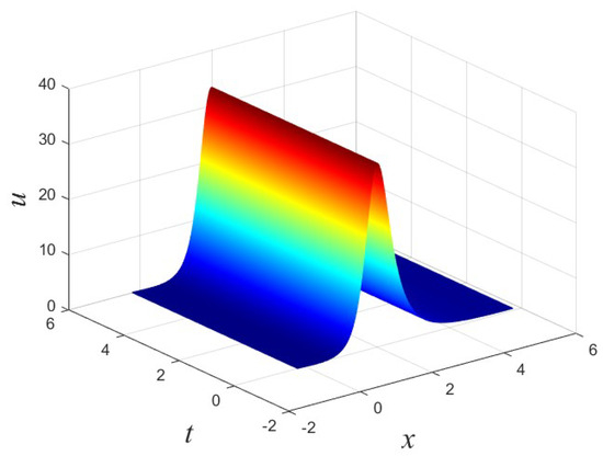
Figure 1.
One-soliton solution of (65) with , , , , .
4. Conclusions and Remarks
In this study, we systematically investigate the Kundu-NLS equation by using the -dressing method. By employing matrix spectral analysis, spectral problems regarding time and space were obtained, which were reduced to Lax pairs of Kundu-NLS equations. In order to obtain the solution, matrix transformation was applied. The soliton solution is obtained by using the -dressing method. In short, the -dressing method is an effective method for solving equations in integrable systems, and this -dressing method shows great potential to address equations in integrable systems in the future.
Author Contributions
Conceptualization, J.H.; methodology, J.H.; formal analysis, J.H.; writing—original draft preparation, J.H.; writing—review and editing, J.H.; funding acquisition, J.H. and N.Z. All authors have read and agreed to the published version of the manuscript.
Funding
This work was supported by the National Natural Science Foundation of China (Nos. 11805114; 1197050803) and the SDUST Research Fund (No. 2018TDJH101).
Institutional Review Board Statement
Not applicable.
Informed Consent Statement
Not applicable.
Data Availability Statement
Data is contained within the article.
Acknowledgments
The authors would like to thank the reviewers and the editor for their valuable comments for improving the original manuscript.
Conflicts of Interest
The authors declare no conflicts of interest.
References
- Kakei, S.; Sasa, N.; Satsuma, J. Bilinearization of a Generalized Derivative Nonlinear Schrödinger Equation. J. Phys. Soc. Jpn. 1995, 64, 1519–1523. [Google Scholar] [CrossRef]
- Sulem, C.; Sulem, P.L. The Nonlinear Schrödinger Equation. In The Nonlinear Schrödinger Equation; Springer: New York, NY, USA, 1999. [Google Scholar]
- Longhi, S. Fractional Schrödinger Equation in Optics. Opt. Lett. 2015, 40, 1117–1120. [Google Scholar] [CrossRef] [PubMed]
- Chekhov, L. A Matrix Model for Classical Nonlinear Schrödinger Equation. Int. J. Mod. Phys. A 1992, 7, 2981–2996. [Google Scholar] [CrossRef]
- Mielnik, B.; Reyes, M.A. The Classical Schrödinger Equation. J. Phys. A-Math. Theor. 1996, 29, 6009–6025. [Google Scholar] [CrossRef]
- Truman, A. Classical Mechanics, the Diffusion (Heat) Equation, and the Schrödinger Equation. J. Math. Phys. 1977, 18, 2308–2315. [Google Scholar] [CrossRef]
- Manikandan, K.; Serikbayev, N.; Manigandan, M.; Sabareeshwaran, M. Dynamical Evolutions of Optical Smooth Positons in Variable Coefficient Nonlinear Schrödinger Equation with External Potentials. Optik 2023, 288, 171203. [Google Scholar] [CrossRef]
- Sabi’u, J.; Tala-Tebue, E.; Rezazadeh, H.; Arshed, S.; Bekir, A. Optical Solitons for the Decoupled Nonlinear Schrödinger Equation Using Jacobi Elliptic Approach. Commun. Theor. Phys. 2021, 73, 075003. [Google Scholar] [CrossRef]
- Rezazadeh, H.; Sabi’u, J.; Jena, R.M.; Chakraverty, S. New Optical Soliton Solutions for Triki–Biswas Model by New Extended Direct Algebraic Method. Mod. Phys. Lett. B 2020, 34, 2150023. [Google Scholar]
- Silem, A.; Lin, J. Exact Solutions for a Variable-Coefficients Nonisospectral Nonlinear Schrödinger Equation via Wronskian Technique. Appl. Math. Lett. 2023, 135, 108397. [Google Scholar] [CrossRef]
- Wang, Z.Y.; Tian, S.F.; Zhang, X.F. Riemann-Hilbert Problem for the Kundu-Type Nonlinear Schrödinger Equation with N Distinct Arbitrary-Order Poles. Theor. Math. Phys. 2021, 207, 415–433. [Google Scholar] [CrossRef]
- Li, J.; Xia, T. A Riemann-Hilbert Approach to the Kundu-Nonlinear Schrödinger Equation and Its Multi-component Generalization. J. Math. Anal. Appl. 2021, 500, 125109. [Google Scholar] [CrossRef]
- Yan, X.W. Riemann–Hilbert Method and Multi-soliton Solutions of the Kundu-Nonlinear Schrödinger Equation. Nonlinear Dyn. 2020, 102, 2811–2819. [Google Scholar] [CrossRef]
- Hu, B.B.; Zhang, L.; Xia, T.C. On the Riemann-Hilbert Problem of a Generalized Derivative Nonlinear Schrödinger Equation. Commun. Theor. Phys. 2021, 73, 015002. [Google Scholar] [CrossRef]
- Zhang, C.; Li, C.; He, J. Darboux Transformation and Rogue Waves of the Kundu-Nonlinear Schrödinger Equation. Math. Method. Appl. Sci. 2015, 38, 2411–2425. [Google Scholar] [CrossRef]
- Wang, X.B.; Han, B. The Kundu-Nonlinear Schrödinger Equation: Breathers, Rogue Waves and Their Dynamics. J. Phys. Soc. Jpn. 2020, 89, 014001. [Google Scholar] [CrossRef]
- Zakharov, V.E.; Shabat, A.B. A Scheme for Integrating the Nonlinear Equations of Mathematical Physics by the Method of the Inverse Scattering Problem (I). Funct. Anal. Appl. 1974, 8, 226–235. [Google Scholar] [CrossRef]
- Zakharov, V.E.; Manakov, S.V. Construction of Higher-dimensional Nonlinear Integrable Systems and of Their Solutions. Funct. Anal. Appl. 1985, 19, 89–101. [Google Scholar] [CrossRef]
- Ablowitz, M.J.; Yaacov, D.B.; Fokas, A.S. On the Inverse Scattering Transform for the Kadomtsev-Petviashvili Equation. Stud. Appl. Math. 1983, 69, 135–143. [Google Scholar] [CrossRef]
- Beals, R.; Coifman, R.R. The Approach to Inverse Scattering and Nonlinear Evolutions. Phys. D 1986, 18, 242–249. [Google Scholar] [CrossRef]
- Beals, R.; Coifman, R.R. Scattering and Inverse Scattering for First-order Systems: II. Inverse. Probl. 1987, 3, 577–593. [Google Scholar] [CrossRef]
- Manakov, S.V. The Inverse Scattering Transform for the Time-dependent Schrödinger Equation and Kadomtsev-Petviashvili Equation. Phys. D 1981, 3, 420–427. [Google Scholar] [CrossRef]
- Konopelchenko, B.G.; Alonso, L.M. Dispersionless Scalar Integrable Hierarchies, Whitham Hierarchy, and the Quasiclassical -dressing Method. J. Math. Phys. 2002, 43, 3807–3823. [Google Scholar] [CrossRef]
- Luo, J.; Fan, E. A -dressing Approach to the Kundu-Eckhaus Equation. J. Geom. Phys. 2021, 167, 1042911. [Google Scholar] [CrossRef]
- Luo, J.; Fan, E. -dressing Method for the Gerdjikov-Ivanov Equation with Nonzero Boundary Conditions. Appl. Math. Lett. 2021, 110, 106589. [Google Scholar] [CrossRef]
- Zhu, Q.; Xu, J.; Fan, E. The Riemann-Hilbert Problem and Long-time Asymptotics for the Kundu-Eckhaus Equation with Decaying Initial Value. Appl. Math. Lett. 2017, 76, 81–89. [Google Scholar] [CrossRef]
- Sun, S.F.; Li, B. A -dressing Method for the Mixed Chen-Lee-Liu Derivative Nonlinear Schrödinger Equation. J. Nonlinear Math. Phys. 2022, 30, 201–214. [Google Scholar] [CrossRef]
- Yang, S.X.; Li, B. A -dressing Method for the (2+1)-Dimensional Korteweg-de Vries Equation. Appl. Math. Lett. 2023, 140, 108589. [Google Scholar] [CrossRef]
- Zhu, J.Y.; Geng, X.G. The AB Equations and the -dressing Method in Semi-characteristic Coordinates. Math. Phys. Anal. Geom. 2014, 17, 49–65. [Google Scholar] [CrossRef]
- Kuang, Y.; Zhu, J.Y. A Three-wave Interaction Model with Self-consistent Sources: The -dressing Method and Solutions. J. Math. Anal. Appl. 2015, 426, 783–793. [Google Scholar] [CrossRef]
Disclaimer/Publisher’s Note: The statements, opinions and data contained in all publications are solely those of the individual author(s) and contributor(s) and not of MDPI and/or the editor(s). MDPI and/or the editor(s) disclaim responsibility for any injury to people or property resulting from any ideas, methods, instructions or products referred to in the content. |
© 2024 by the authors. Licensee MDPI, Basel, Switzerland. This article is an open access article distributed under the terms and conditions of the Creative Commons Attribution (CC BY) license (https://creativecommons.org/licenses/by/4.0/).