Approximate Analytical Solutions for Strongly Coupled Systems of Singularly Perturbed Convection–Diffusion Problems

Abstract

This work presents a reliable algorithm to obtain approximate analytical solutions for a strongly coupled system of singularly perturbed convection–diffusion problems, which exhibit a boundary layer at one end. The proposed method involves constructing a zero-order asymptotic approximate solution for the original system. This approximation results in the formation of two systems: a boundary layer system with a known analytical solution and a reduced terminal value system, which is solved analytically using an improved residual power series approach. This approach combines the residual power series method with Padé approximation and Laplace transformation, resulting in an approximate analytical solution with higher accuracy compared to the conventional residual power series method. In addition, error estimates are extracted, and illustrative examples are provided to demonstrate the accuracy and effectiveness of the method.

1. Introduction

Singular perturbation problems (SPPs) arise in diversified areas of applied mathematics and engineering, such as aerodynamics, fluid mechanics, elasticity, optimal control and more [1,2,3,4,5,6,7]. It is widely recognized that solutions to such problems exhibit a multiscale nature, characterized by the presence of thin layers where the solution undergoes rapid variations, while outside of these layers, the solution behaves smoothly and changes slowly. Numerous analytical and numerical approaches have been developed to handle and solve SPPs, as examined in the studies conducted by O’Malley [6], Miller et al. [7], Ross et al. [8] and other referenced works [9,10,11,12,13,14,15,16,17,18,19,20,21,22,23,24,25,26,27,28,29,30,31,32,33,34,35,36,37].

Traditional numerical methods often struggle to provide accurate approximate solution of SPPs due to the presence of thin layer regions. To overcome this challenge, some numerical techniques treat second-order singularly perturbed boundary value problems (SPBVPs) by transforming them into appropriate initial value problems (IVPs). This is because that the numerical treatment of corresponding IVPs is comparatively easier than that of BVPs. Various initial value techniques for solving SPBVPs have been developed in the literature, as discussed in papers [9,10,11,12,13,14,15].

While there are many works on SPPs in the literature, most of the computational aspects have focused on second-order SPBVPs. Only a few works have been reported for higher orders and systems of SPBVPs although these problems have many applications [1,2,3,4,5]. In recent years, non-classical methods have been developed for different classes of singularly perturbed boundary value systems (SPBVSs). Some scholars have studied a class of reaction–diffusion SPBVSs [16,17,18,19,20,21], while others have examined strongly coupled convection–diffusion SPBVSs [22,23,24,25,26,27,28,29,30,31], and weakly coupled SPBVS have been considered in [32,33,34]. However, most methods developed for SPBVSs are based on numerical fitted mesh methods, underscoring the demand for alternative approaches that provide accurate approximate analytical solutions.

Among different methods that have been developed to obtain analytical approximations for the solutions to differential equations, we can use the homotopy analysis method [37,38,39,40], homotopy perturbation method [41,42], differential transform method [43,44,45,46,47,48] and residual power series method (RPSM) [49,50,51,52,53,54,55], among others.

The RPSM is a powerful technique for solving IVPs without linearization, perturbation or discretization [49,50,51,52,53,54,55,56,57,58]. It stands apart from classical power series methods, which can be computationally expensive. However, the RPSM and other Taylor series approximation methods face limitations and challenges, particularly when applied to problems that span a substantial time interval or involve high solution gradients, such as those containing boundary layers [52,53,54]. To overcome this, an enhanced version of the RPSM called the improved RPSM (IRPSM) is proposed. The IRPSM utilizes Padé approximants, which are known for their superior convergence compared to series approximations [37,45,56,57,58,59,60]. Moreover, by combining the Laplace transform method with Padé approximations [42,52,56], we can obtain more accurate solutions that closely approach exact solutions.

This paper presents an efficient algorithm designed to obtain approximate analytical solutions for a complex system of strongly coupled singularly perturbed convection–diffusion problems. These problems exhibit a boundary layer phenomenon at one end, which poses significant challenges in finding accurate solutions. The proposed method involves constructing a zero-order asymptotic approximate solution for the given system, followed by the analytical solution of the reduced terminal value system (RTVS) using the IRPSM technique. To improve accuracy and convergence properties of RPSMs, the IRPSM combines an RPSM with Padé approximation and Laplace transformation. Compared to the conventional RPSM method, the proposed IRPSM offers higher accuracy and a larger convergence region. This paper also addresses error estimation and demonstrates the effectiveness of the present method through illustrative examples.

2. Description of the Method

Consider the following strongly coupled system of two singularly perturbed convection–diffusion boundary value problems [24,29,30]

$$\left\{\begin{array}{c}\epsilon y_1^{″}+a_{11}{y}_1^{\prime }+a_{12}{y}_2^{\prime }+b_{11}{y}_1+b_{12}{y}_2=f_1 \\ \epsilon y_2^{″}+a_{21}{y}_1^{\prime }+a_{22}{y}_2^{\prime }+b_{21}{y}_1+b_{22}{y}_2=f_2 \end{array}\right..$$

(1)

with the following Dirichlet boundary conditions

$$y_i\left(a\right)={\alpha }_i \mathrm{and} y_i\left(b\right)={\beta }_i \mathrm{for} i=1,2.$$

(2)

where $0<\epsilon \ll 1$, $y_i=y_i\left(x\right)$, $a_{ij}=a_{ij}\left(x\right)$, $b_{ij}=b_{ij}\left(x\right)$ and $f_i=f_i\left(x\right)$ for $i=1,2$ are assumed to be sufficiently continuously differentiable functions for $x\in \left(a,b\right)$, with $a_{ii}>0, a_{ij}\le 0, i\ne j$, and with ${\alpha }_i$, ${\beta }_i$ as given constants [24,29,30]. Under these conditions, the problem exhibits overlapping boundary layers at $x=a$ with a width of $\mathrm{O}\left(\epsilon \right)$ [24]. The equations in (1) are strongly coupled through their convective terms [22]. The analytical behavior of the solution to the SPBVS (1) is influenced by the nature of the boundary conditions, and it has been noted in [8] that the most challenging case arises when these conditions are of the Dirichlet type, like those described in (2). For more details about analytical results such as existence, uniqueness and asymptotic solution approximation, one may refer to the work presented in Refs. [22,23,24,25,26,27,28,29,30,31].

The coupled SPBVS (1)–(2) finds numerous practical applications in modeling complex physical phenomena [1,2,3,4,5,25]. These include the turbulent interaction of waves and currents [2], diffusion processes involving chemical reactions [3], optimal control problems in resistance–capacitor electrical circuits [1], magnetohydrodynamic duct flow problems [4,5,61,62] and more. Obtaining accurate analytical solutions for this SPBVS is crucial as it allows researchers to carefully study how different physical parameters affect the behavior of the solutions. Having these solutions available helps improve our understanding and analysis of the system’s dynamics, leading to advancements in scientific knowledge.

2.1. A Zeroth-Order Asymptotic Expansion

By applying well-known perturbation methods [6,7,8,35,36], it is possible to construct an asymptotic expansion for the solution of the SPBVS (1)–(2). Let $\overrightarrow{u}={\left(u_1,u_2\right)}^T$ denote the solution of the RTVS associated with the SPBVS (1)–(2), and subject to

$$\left\{\begin{array}{c}{a}_{11}{u}_1^{\prime }+a_{12}{u}_2^{\prime }+b_{11}{u}_1+b_{12}{u}_2=f_1,\\ a_{21}{u}_1^{\prime }+a_{22}{u}_2^{\prime }+b_{21}{u}_1+b_{22}{u}_2=f_2\\ u_i\left(b\right)={\beta }_i,\hspace{1em}i=\mathrm{1,2}.\hfill \end{array}\right.,$$

(3)

the solution of RTVS (3) satisfies the original SPBVS (1)–(2) on most of the interval $\left[a,b\right]$ and away from $x=a$ [6,7,8,35,36].

Further, the SPBVS (1)–(2) can be written as follows:

$$\left\{\begin{array}{l}\epsilon y_1^{″}+{\left(a_{11}{y}_1\right)}^{\prime }+{\left(a_{12}{y}_2\right)}^{\prime }=F\left(x,y_1,y_2\right),\\ \epsilon y_2^{″}+{\left(a_{21}{y}_1\right)}^{\prime }+{\left(a_{22}{y}_2\right)}^{\prime }=G\left(x,y_1,y_2\right)\\ y_i\left(a\right)={\alpha }_i and y_i\left(b\right)={\beta }_i for i=1,2.\end{array}\right. ,$$

(4)

where

$$F\left(x,y_1,y_2\right)=f_1+a_{11}^{\prime }{y}_1+a_{12}^{\prime }{y}_2-b_{11}{y}_1-b_{12}{y}_2,$$

$$G\left(x,y_1,y_2\right)=f_2+a_{21}^{\prime }{y}_1+a_{22}^{\prime }{y}_2-b_{21}{y}_1-b_{22}{y}_2.$$

Through the process of substitution, specifically by replacing the solutions $y_1 \mathrm{a}\mathrm{n}\mathrm{d} y_2$ with $u_1 \mathrm{a}\mathrm{n}\mathrm{d} u_2$, respectively, on the right-hand side of Equation (4), an asymptotically equivalent approximation is obtained. This substitution technique has been discussed and referenced in previous works [5,10,12,13,14,15,35,36].

$$\left\{\begin{array}{c} \epsilon y_1^{″}+{\left(a_{11}{y}_1\right)}^{\prime }+{\left(a_{12}{y}_2\right)}^{\prime }=F\left(x,u_1,u_2\right)+O\left(\epsilon \right),\\ \epsilon y_2^{″}+{\left(a_{21}{y}_1\right)}^{\prime }+{\left(a_{22}{y}_2\right)}^{\prime }=G\left(x,u_1,u_2\right)+O\left(\epsilon \right),\\ y_i\left(a\right)={\alpha }_i and y_i\left(b\right)={\beta }_i, i=\mathrm{1,2}.\hfill \end{array}\right.$$

(5)

By utilizing the RTVS (3), the SPBVS (5) can be reformulated as follows:

$$\left\{\begin{array}{l}\epsilon y_1^{″}+{\left(a_{11}{y}_1\right)}^{\prime }+{\left(a_{12}{y}_2\right)}^{\prime }={\left(a_{11}{u}_1\right)}^{\prime }+{\left(a_{12}{u}_2\right)}^{\prime }+O\left(\epsilon \right), \\ \epsilon y_2^{″}+{\left(a_{21}{y}_1\right)}^{\prime }+{\left(a_{22}{y}_2\right)}^{\prime }={\left(a_{21}{u}_1\right)}^{\prime }+{\left(a_{22}{u}_2\right)}^{\prime }+O\left(\epsilon \right) \\ y_i\left(a\right)={\alpha }_i and y_i\left(b\right)={\beta }_i, i=\mathrm{1,2}.\hfill \end{array}\right.,$$

(6)

By integrating (6) from $b$ to $x$, we obtain the following singularly perturbed initial value system:

$$\left\{\begin{array}{l}\epsilon y_1^{\prime }+a_{11}\left(y_1-u_1\right)+a_{12}{(y}_2-u_2)=O(\epsilon )+K_1, \\ \epsilon y_2^{\prime }+a_{21}{(y}_1-u_1)+a_{22}{(y}_2-u_2)=O\left(\epsilon \right)+K_2,\\ \hspace{1em}{y}_i\left(a\right)={\alpha }_i, i=\mathrm{1,2} , \end{array}\right.$$

(7)

where $K_i, i=\mathrm{1,2}$ are constants of the integration and

• $K_i=-\left(\epsilon y_i^{\prime }\left(b\right)+a_{i1}\left(y_1\left(b\right)-u_1\left(b\right)\right)+a_{i2}{(y}_2\left(b\right)-u_2\left(b\right))\right), i=\mathrm{1,2}.,\mathrm{i}.\mathrm{e}.$,
• $K_i=\epsilon y_i^{\prime }\left(b\right)=O\left(\epsilon \right)$ [10,12,13,14,15,35,36].

Now, let $y_i\left(x\right){=u}_i\left(x\right){+v}_i\left(t\right)+O\left(\epsilon \right), i=\mathrm{1,2}$, where $t=\left(x-a\right)/\epsilon$ [10,13,15,35,36]; then, the SPBVS (7) results in the following linear layer correction problem:

$$\left\{\begin{array}{l}{\dot{v}}_1+a_{11}\left(a\right)v_1\left(t\right)+a_{12}\left(a\right)v_2\left(t\right)=O\left(\epsilon \right),\\ {\dot{v}}_2+a_{21}\left(a\right)v_1\left(t\right)+a_{22}\left(a\right)v_2\left(t\right)=O\left(\epsilon \right),\\ v_i\left(a\right)={\alpha }_i-u_i\left(a\right),i=\mathrm{1,2}. \end{array}\right.$$

(8)

with the asymptotic approximate solution given by

$$\left\{\genfrac{}{}{0pt}{}{v_1\left(t\right)=\frac{\left({\mathrm{e}}^{\frac{1}{2}t\sqrt{\phi }}\left(\delta \sqrt{\phi }-{\gamma }_1\right)+\left(\delta \sqrt{\phi }+{\gamma }_1\right){\mathrm{e}}^{-\frac{1}{2}t\sqrt{\phi }}\right){\mathrm{e}}^{-\frac{1}{2}t\left(a_{11}\left(a\right)-a_{22}\left(a\right)\right)}}{2\sqrt{\phi }}+O\left(\epsilon \right),}{v_2\left(t\right)=\frac{\left({\mathrm{e}}^{\frac{1}{2}t\sqrt{\phi }}\left(\mu \sqrt{\phi }+{\gamma }_2\right)+\left(\mu \sqrt{\phi }-{\gamma }_2\right){\mathrm{e}}^{-\frac{1}{2}t\sqrt{\phi }}\right){\mathrm{e}}^{-\frac{1}{2}t\left(a_{11}\left(a\right)-a_{22}\left(a\right)\right)}}{2\sqrt{\phi }}+O\left(\epsilon \right).}\right.$$

(9)

where $\delta ={\alpha }_1-u_1\left(a\right),\mu ={\alpha }_2-u_2\left(a\right)$, $\phi ={a_{11}\left(a\right)}^2-2a_{22}\left(a\right)a_{11}\left(a\right)+{a_{22}\left(a\right)}^2+4a_{12}\left(a\right)a_{21}\left(a\right)$, ${\gamma }_1=\left(a_{11}\left(a\right)-a_{22}\left(a\right)\right)\delta +2a_{12}\left(a\right)\mu$ and ${\gamma }_2=\left(a_{11}\left(a\right)-a_{22}\left(a\right)\right)\mu -2a_{21}\left(a\right)\delta$.

Thus, we have $y_i\left(x\right)=y_{i,as}\left(x\right)+O\left(\epsilon \right){, \mathrm{where} y_{i,as}\left(x\right)=u}_i\left(x\right){+v}_i\left(t\right)$, $i=1,2.$

From the above steps, we have proved the following theorem.

Theorem 1.

The solution $\overrightarrow{y}\left(x\right)={\left(\hspace{0.17em}{y}_1\left(x\right),y_2\left(x\right)\right)}^T$ of (1) has a zero-order asymptotic approximation ${\overrightarrow{y}}_{as}\left(x\right)={\left(\hspace{0.17em}{y}_{1,as}\left(x\right),y_{2,as}\left(x\right)\right)}^T$, where

$$\left\{\genfrac{}{}{0pt}{}{y_{1,as}\left(x\right)=u_1\left(x\right)+\frac{\left(e^{\frac{x-a}{2\epsilon }\sqrt{\phi }}\left(\delta \sqrt{\phi }-{\gamma }_1\right)+\left(\delta \sqrt{\phi }+{\gamma }_1\right)e^{\frac{a-x}{2\epsilon }\sqrt{\phi }}\right)e^{\frac{a-x}{2\epsilon }\left(a_{11}\left(a\right)-a_{22}\left(a\right)\right)}}{2\sqrt{\phi }},}{y_{2,as}\left(x\right)=u_2\left(x\right)+\frac{\left(e^{\frac{x-a}{2\epsilon }\sqrt{\phi }}\left(\mu \sqrt{\phi }+{\gamma }_2\right)+\left(\mu \sqrt{\phi }-{\gamma }_2\right)e^{\frac{a-x}{2\epsilon }\sqrt{\phi }}\right)e^{\frac{a-x}{2\epsilon }\left(a_{11}\left(a\right)-a_{22}\left(a\right)\right)}}{2\sqrt{\phi }} ,}\right.$$

(10)

and

$$‖\hspace{0.17em}\overrightarrow{y}\left(x\right)-{ \overrightarrow{y}}_{as}\left(x\right)\hspace{0.17em}\hspace{0.17em}‖\le C_1\hspace{0.17em}\epsilon .$$

Now, to obtain an approximate analytical solution of the SPBVS (1)–(2), we only need to obtain an approximate analytical solution of the RTVS (3).

2.2. RPSM for the RTVS (3)

In this subsection, the RPSM is introduced for solving the RTVS (3). The RPSM consists of expressing the solution of the RTVS (3) as a power series expansion about the terminal point $x=b$ [49,55]. To achieve our goal, we suppose that the solution of the RTVS (3) takes the following form:

$$u_i\left(x\right)={\sum }_{n=0}^{\mathrm{\infty }}{c}_{i,n}{\left(x-b\right)}^n,i=\mathrm{1,2}.$$

(11)

and can be approximated using the following $k^{th}$ truncated series.

$$u_i^k\left(x\right)={\sum }_{n=0}^k{c}_{i,n}{\left(x-b\right)}^n,i=\mathrm{1,2}.$$

(12)

Applying the RPSM to the RTVS (3) leads to the following definitions of the $k^{th}$-residual functions and the ${\infty }^{th}$-residual functions, respectively, as proposed by [49,51,53,55]:

$${\overrightarrow{Res}}_x^k=A \frac{d}{dx} \overrightarrow{u}+B \overrightarrow{u}-\overrightarrow{f},$$

(13)

where ${\overrightarrow{Res}}_x^k=\left(\genfrac{}{}{0pt}{}{{Res}_1^k\left(x\right)}{{Res}_2^k\left(x\right)}\right)$, $\overrightarrow{u}=\left(\genfrac{}{}{0pt}{}{u_1\left(x\right)}{u_2\left(x\right)}\right)$, $A=\left(\genfrac{}{}{0pt}{}{a_{11}}{a_{21}}\genfrac{}{}{0pt}{}{a_{12}}{a_{22}}\right)$, $B=\left(\genfrac{}{}{0pt}{}{b_{11}}{b_{21}}\genfrac{}{}{0pt}{}{b_{12}}{b_{22}}\right)$ and $\overrightarrow{f}=\left(\genfrac{}{}{0pt}{}{f_1}{f_2}\right)$.

$${\overrightarrow{Res}}_x^{\mathrm{\infty }}=\underset{k\to \mathrm{\infty }}{\mathit{lim}}{\overrightarrow{Res}}_x^k=A \frac{d}{dx} \overrightarrow{u}+B \overrightarrow{u}-\overrightarrow{f}.$$

(14)

It is easy to see that ${\overrightarrow{Res}}_x^{\infty }=0$ for each $x\in \left[a,b\right]$ are infinitely differentiable functions at $x=b$. Moreover,

$${\frac{d^m}{{dx}^m}\overrightarrow{Res}}_b^k={\frac{d^m}{{dx}^m}\overrightarrow{Res}}_b^{\mathrm{\infty }},m=\mathrm{1,2},..,k,$$

(15)

which is a basic rule in the RPSM.

By using (15), the unknown coefficients $c_{i,n},i=1,2, \mathrm{and} n=0...k$ are determined and the approximate series solution (12) is obtained [49,50,51,52,53,54,55].

3. Improved RPSM

To enhance the accuracy and expand the convergence region of the series solution obtained from the RPSM, we recommend employing the Laplace–Padé combination approach for the truncated series solution of the RPSM (12). We assume that the solution of the RTVS (3) and its corresponding series expansion (12) satisfy the conditions of Laplace transformability and a Padé approximant [42,52,56,57,58,59,60].

3.1. Padé Approximant at $x=b$

Padé approximants are the best rational approximations of power series [57,58,59,60]. The truncated power series solution $u_i^k\left(x\right)$ defined by (12) can by approximated through Padé approximation as follows [37,56,57,58,59,60]:

Let the rational approximation of $u_i^k\left(x\right)$ be the quotient of two polynomials $p_{i,l}\left(x\right)$ and $q_{i,m}\left(x\right)$ of degrees $l$ and $m$, respectively, as defined by

$$u_i^{l,m}\left(x\right)=\frac{P_{i,l}\left(x\right)}{Q_{i,m}\left(x\right)}, i=\mathrm{1,2} \mathrm{a}\mathrm{n}\mathrm{d} l+m\le k,$$

(16)

where

$$P_{i,l}\left(x\right)={\sum }_{r=0}^l{p}_{i,r}{\left(x-b\right)}^r,\hspace{0.17em}{Q}_{i,m}\left(x\right)={\sum }_{r=0}^m{q}_{i,r}{\left(x-b\right)}^r,q_{i,0}=1,i=1,2.$$

(17)

The polynomials in (17) are constructed so that $u_i\left(x\right)$ and $u_i^{l,m}\left(x\right)$ agree at $x=b$ and their derivatives up to $l+m\le k$. Consequently, the subsequent expression

$$u_i\left(x\right)-\frac{P_{i,l}\left(x\right)}{Q_{i,m}\left(x\right)}=O\left({\left(x-b\right)}^{l+m+1}\right),$$

(18)

determines the coefficients of $P_{i,l}\left(x\right)$ and $Q_{i,m}\left(x\right)$ [37,56,57,58,59,60]. Multiplying (18) by $Q_{i,m}\left(x\right)$ results in

$$\left({\sum }_{r=0}^{\infty }{c}_{i,r}{\left(x-b\right)}^n \right)\left({\sum }_{r=0}^m{q}_{i,r}{\left(x-b\right)}^r\right)-\left({\sum }_{j=0}^l{p}_{i,j}{\left(x-b\right)}^j\right)={\sum }_{r=l+m+1}^{\infty }{c}_{i,r}{\left(x-b\right)}^r, i=\mathrm{1,2}.$$

(19)

When the left side of (19) is multiplied out and the coefficients of the powers of ${\left(x-b\right)}^r$ are set equal to zero for $r=0, 1,\dots ,l+m$, the result is a system of $2\left(l+m+1\right)$ linear equations in the $2\left(l+m+1\right)$ unknown coefficients of $P_{i,l}\left(x\right)$ and $Q_{i,m}\left(x\right)$. By solving this linear system, we obtain the rational approximation $u_i^{l,m}\left(x\right)$.

Although Padé approximation $u_i^{l,m}\left(x\right)$ agree with truncated Taylor expansions $u_i^{l+m}\left(x\right)$ up to order $O(l+m)$, Padé approximation can outperform truncated Taylor expansion because it can accurately represent functions with poles or singularities outside the region of convergence of a Taylor expansion, resulting in more accurate approximation and a larger convergence region [42,52,56,57,58,59,60].

3.2. Laplace–Padé Algorithm

The Laplace–Padé$\left[\frac{l}{m}\right]$ algorithm can be described as follows:

• Step 1. Begin by replacing $x-b \mathrm{w}\mathrm{i}\mathrm{t}\mathrm{h} t$ in the power series (12) and then apply Laplace transformation, resulting in a transformed series $U_i\left(s\right), i=1, 2$.
• Step 2. Substitute $s$ with $1/\tau$ in the transformed series $U_i\left(s\right)$.
• Step 3. Convert the resulting series into a Padé approximant $u_i^{l,m}\left(\tau \right)$.
• Step 4. Replace $\tau$ with $1/s$ in $u_i^{l,m}\left(\tau \right)$.
• Step 5. Lastly, apply the inverse Laplace transform and replace $t$ with $x-b$ to obtain the approximate augmented solution $u_{i,ap}\left(x\right)$, $i=1, 2.$

Finally, the approximate analytical solution of the SPBVS (1)–(2) can be expressed by

$$\genfrac{}{}{0pt}{}{y_{1,ap}\left(x\right)=u_{1,ap}\left(x\right)+\frac{\left(e^{\frac{x-a}{2\epsilon }\sqrt{\phi }}\left(\delta \sqrt{\phi }-{\gamma }_1\right)+\left(\delta \sqrt{\phi }+{\gamma }_1\right)e^{\frac{a-x}{2\epsilon }\sqrt{\phi }}\right)e^{\frac{a-x}{2\epsilon }\left(a_{11}\left(a\right)-a_{22}\left(a\right)\right)}}{2\sqrt{\phi }},}{y_{2,ap}\left(x\right)=u_{2,ap}+\frac{\left(e^{\frac{x-a}{2\epsilon }\sqrt{\phi }}\left(\mu \sqrt{\phi }+{\gamma }_2\right)+\left(\mu \sqrt{\phi }-{\gamma }_2\right)e^{\frac{a-x}{2\epsilon }\sqrt{\phi }}\right)e^{\frac{a-x}{2\epsilon }\left(a_{11}\left(a\right)-a_{22}\left(a\right)\right)}}{2\sqrt{\phi }}.}$$

(20)

3.3. Error Estimate of the Method

The numerical error of the present method has two sources: one from the asymptotic approximation and the other from the analytical approximation by the IRPSM.

Theorem 2.

The solution $\overrightarrow{y}\left(x\right)={\left(\hspace{0.17em}{y}_1\left(x\right),y_2\left(x\right)\right)}^T$ of (1) and the approximate analytical solution${ \overrightarrow{y}}_{ap}\left(x\right)={\left(\hspace{0.17em}{y}_{1,ap}\left(x\right),y_{2,ap}\left(x\right)\right)}^T$in (20) satisfy the inequality.

$$‖\hspace{0.17em}\hspace{0.17em}\overrightarrow{y}\left(x\right)-{ \overrightarrow{y}}_{ap}\left(x\right)\hspace{0.17em}\hspace{0.17em}‖\le \mathrm{C}\hspace{0.17em}\left(\epsilon +\frac{1}{\left(l+m+1\right)!}\right).$$

(21)

Proof.

We have

$$‖\hspace{0.17em}\hspace{0.17em}\overrightarrow{y}\left(x\right)-{ \overrightarrow{y}}_{ap}\left(x\right)\hspace{0.17em}\hspace{0.17em}‖\le ‖\hspace{0.17em}\hspace{0.17em}\hspace{0.17em}\overrightarrow{y}\left(x\right)-{ \overrightarrow{\mathrm{y}}}_{as}\left(x\right)\hspace{0.17em}\hspace{0.17em}‖+‖\hspace{0.17em}{ \overrightarrow{\mathrm{y}}}_{as}\left(x\right)-{ \overrightarrow{y}}_{ap}\left(x\right)‖,$$

and

$$\begin{array}{c}‖\hspace{0.17em}{ \overrightarrow{\mathrm{y}}}_{as}\left(x\right)-{ \overrightarrow{y}}_{ap}\left(x\right)‖\le ‖\hspace{0.17em}\hspace{0.17em}\overrightarrow{u}\left(x\right)-{\overrightarrow{u}}_{ap}\left(x\right)‖\le ‖\hspace{0.17em}\hspace{0.17em}\overrightarrow{u}\left(x\right)-{\overrightarrow{u}}^{l,m}\left(x\right)‖,\\ \le ‖\hspace{0.17em}\hspace{0.17em}\overrightarrow{u}\left(x\right)-{\overrightarrow{u}}^{l,m}\left(x\right)‖,\end{array}$$

where ${\overrightarrow{u}}_{ap}\left(x\right)={\left(\hspace{0.17em}{u}_{1,ap}\left(x\right),u_{2,ap}\left(x\right)\right)}^T$ and ${\overrightarrow{u}}^{l,m}\left(x\right)={\left(\hspace{0.17em}{u}_1^{l,m}\left(x\right),u_2^{l,m}\left(x\right)\right)}^T$.

And since Padé approximant ${\overrightarrow{u}}^{l,m}\left(x\right)$ has a bounded error given by [57,58,59,60]

$$‖\hspace{0.17em}\hspace{0.17em}\overrightarrow{u}\left(x\right)-{\overrightarrow{u}}^{l,m}\left(x\right)‖\le \frac{T}{\left(l+m+1\right)!}, T\le ‖\hspace{0.17em}{u}^{\left(l+m+1\right)}\left(\pi \right)‖, 0\le \pi \le 1 ,$$

then, from Theorem 1 and the above bounded errors, we have

$$‖\hspace{0.17em}\hspace{0.17em}\overrightarrow{y}\left(x\right)-{ \overrightarrow{y}}_{ap}\left(x\right)\hspace{0.17em}\hspace{0.17em}‖\le \mathrm{C}\hspace{0.17em}\left(\epsilon +\frac{1}{\left(l+m+1\right)!}\right).$$

It is worth highlighting that the IRPSM often provides the exact solution for the RTVS (3) and eliminates the second term in the error inequality (21). Conversely, when the asymptotic boundary layer solution (9) accurately represents the boundary layer solution of the original SPBVS (1)–(2), the first term in the error inequality (21) is eliminated. In such a case, the remaining error becomes independent of the perturbation parameter ε and is solely determined by the methods used to solve the RTVS (3). □

4. Numerical Results

This section provides illustrative examples that demonstrate the method’s accuracy and efficiency in solving the considered problems. The selected examples have been carefully chosen from the literature and have known exact solutions, allowing for a comprehensive comparison. They include both two- and three-dimensional linear examples with constant or variable coefficients. Furthermore, these examples involve non-homogeneous source terms that can be constant, exponential or trigonometric in nature. Additionally, we have considered examples with both Dirichlet and Robin boundary conditions, and we have included cases with known or unknown exact solutions. These selections aim to facilitate a thorough analysis of the proposed method and provide a comprehensive understanding of its applicability and effectiveness. Throughout this section, we will refer to the combination of the asymptotic approximation and RPSM as A-RPSM, and the combination of the asymptotic approximation and IRPSM as A-IRPSM. All symbolic calculations were conducted using MAPLE 14, while numerical simulations were performed using MATLAB 2017b.

Example 1.

Consider the following SPBVS [24,32]

$$\left\{\begin{array}{c}\epsilon {y^{″}}_1\left(x\right)+{y^{\prime }}_1\left(x\right)-2y_1\left(x\right)+y_2\left(x\right)=f_1\left(x\right) , \\ \epsilon {y^{″}}_2\left(x\right)+2{y^{\prime }}_2\left(x\right)+y_1\left(x\right)-4y_2\left(x\right)=f_2\left(x\right) ,\end{array}\right.$$

(22)

with Dirichlet boundary conditions

$$y_1(0)=y_1(1)=y_2(0)=y_2(1)=0,$$

and where $f_1\left(x\right) and f_2\left(x\right)$ are given by

$$f_1\left(x\right)=\frac{4{\mathrm{e}}^{-\frac{x}{\mathsf{\epsilon }}}-\mathrm{s}\mathrm{i}\mathrm{n}\left(\frac{\mathsf{\pi }x}{2}\right){\mathsf{\pi }}^2{\mathsf{\epsilon }}^2\left(1-{\mathrm{e}}^{-\frac{1}{\mathsf{\epsilon }}}\right)}{2\mathsf{\epsilon }\left(-1+{\mathrm{e}}^{-\frac{1}{\mathsf{\epsilon }}}\right)}+\frac{2{\mathrm{e}}^{-\frac{x}{\mathsf{\epsilon }}}}{\mathsf{\epsilon }\left(1-{\mathrm{e}}^{-\frac{1}{\mathsf{\epsilon }}}\right)}-\mathsf{\pi }\mathrm{c}\mathrm{o}\mathrm{s}\left(\frac{\mathsf{\pi }x}{2}\right)+\frac{4-4{\mathrm{e}}^{-\frac{x}{\mathsf{\epsilon }}}}{-1+{\mathrm{e}}^{-\frac{1}{\mathsf{\epsilon }}}}+4\mathrm{s}\mathrm{i}\mathrm{n}\left(\frac{\mathsf{\pi }x}{2}\right)+\frac{1-{\mathrm{e}}^{-\frac{2x}{\mathsf{\epsilon }}}}{1-{\mathrm{e}}^{-\frac{2}{\mathsf{\epsilon }}}}-x{\mathrm{e}}^{x-1},$$

$$f_2\left(x\right)=\frac{-4{\mathrm{e}}^{-\frac{2x}{\mathsf{\epsilon }}}-{\mathrm{e}}^{x-1}{\mathsf{\epsilon }}^2\left(1-{\mathrm{e}}^{-\frac{2}{\mathsf{\epsilon }}}\right)\left(x+2\right)}{\mathsf{\epsilon }\left(1-{\mathrm{e}}^{-\frac{2}{\mathsf{\epsilon }}}\right)}+\frac{4{\mathrm{e}}^{-\frac{2x}{\mathsf{\epsilon }}}}{\mathsf{\epsilon }\left(1-{\mathrm{e}}^{-\frac{2}{\mathsf{\epsilon }}}\right)}+2\left(x-1\right){\mathrm{e}}^{x-1}+\frac{2-2{\mathrm{e}}^{-\frac{x}{\mathsf{\epsilon }}}}{1-{\mathrm{e}}^{-\frac{1}{\mathsf{\epsilon }}}}-2\mathrm{s}\mathrm{i}\mathrm{n}\left(\frac{\mathsf{\pi }x}{2}\right)+\frac{4-4{\mathrm{e}}^{-\frac{2x}{\mathsf{\epsilon }}}}{-1+{\mathrm{e}}^{-\frac{2}{\mathsf{\epsilon }}}}.$$

The exact solution to SPBVS (22) is given by

$$\begin{array}{l}{y}_1(x)=2\left(\frac{1-e^{-x/\epsilon }}{1-e^{-1/\epsilon }}-\sin \left(\frac{\pi x}{2}\right)\right)\hspace{0.17em}\hspace{0.17em},\\ y_2(x)=\frac{1-e^{-2x/\epsilon }}{1-e^{-2/\epsilon }}-x{e}^{x-1}\hspace{0.17em}\hspace{0.17em}\hspace{0.17em}.\end{array}$$

The RTVS of (22) is given by

$$\begin{array}{l}{u^{\prime }}_1\left(x\right)-2u_1\left(x\right)+u_2\left(x\right)=4sin\left(\frac{\pi x}{2}\right)-\pi \mathrm{c}\mathrm{o}\mathrm{s}\left(\frac{\pi x}{2}\right)-3-x{\mathrm{e}}^{x-1} , \\ 2{u^{\prime }}_2\left(x\right)+u_1\left(x\right)-4u_2\left(x\right)=2\left(x-1\right){\mathrm{e}}^{x-1}-2sin\left(\frac{\pi x}{2}\right)-2 .\\ u_1\left(1\right)=u_2\left(1\right)=0 . \end{array}$$

(23)

When applying the RPSM with the 10th order to the RTVS (23), the result series solution is given by

$$\left\{\begin{array}{c}{u}_1^{10}=\frac{1}{4}{\pi }^2{\left(x-1\right)}^2-\frac{1}{192}{\pi }^4{\left(x-1\right)}^4+\frac{1}{23040}{\pi }^6{\left(x-1\right)}^6-\frac{1244}{676631}{\left(x-1\right)}^8++\frac{139}{2757713}{\left(x-1\right)}^{10} \\ +O\left({\left(x-1\right)}^{11}\right) ,\\ u_2^{10}=-2\left(x-1\right)-\frac{3}{2}{\left(x-1\right)}^2-\frac{2}{3}{\left(x-1\right)}^3-\frac{5}{24}{\left(x-1\right)}^4-\frac{1}{20}{\left(x-1\right)}^5-\frac{7}{720}{\left(x-1\right)}^6-\\ -\frac{1}{630}{\left(x-1\right)}^7-\frac{1}{4480}{\left(x-1\right)}^8-\frac{1}{36288}{\left(x-1\right)}^9-\frac{11}{3628800}{\left(x-1\right)}^{10}+O\left({\left(x-1\right)}^{11}\right) .\end{array}\right.$$

(24)

When applying the Laplace–Padé [5/5] algorithm to (24), this results in

$$\begin{array}{c}{u}_{1,ap}=\frac{250000000000001}{125000000000000}-\frac{7}{22637359266701}\cos \left(\frac{37404834}{24569305}x-\frac{37404834}{24569305}\right)\hfill \\ -\frac{6644518272423}{3322259136212}\cos \left(\frac{75297710}{47936011}x-\frac{75297710}{47936011}\right), \\ u_{2,ap}=1-x{\mathrm{e}}^{x-1} . \hfill \end{array}$$

(25)

Thus, we have an approximate analytical solution to the SPBVS (22), given by

$$\begin{array}{c}{y}_{1,ap}=\frac{250000000000001}{125000000000000}-\frac{7}{22637359266701}\cos \left(\frac{37404834}{24569305}x-\frac{37404834}{24569305}\right)\hfill \\ -\frac{6644518272423}{3322259136212}\cos \left(\frac{75297710}{47936011}x-\frac{75297710}{47936011}\right)-2{\mathrm{e}}^{-\frac{x}{\epsilon }} , \\ y_{2,ap}=1-x{\mathrm{e}}^{x-1}-{\mathrm{e}}^{-\frac{2x}{\epsilon }} . \hfill \end{array}$$

(26)

To portray the solution behavior inside the boundary layer, Figure 1 presents the profiles of the exact solution (solid line) and the approximate solution (dotted marked line) in Example 1 over (left) the problem domain $\left[0, 1\right]$ and (right) a boundary layer region for different values of $\epsilon$. This shows that the solution exhibits a high gradient within the boundary layer, which poses a challenge for classical numerical methods to accurately capture without special treatment.

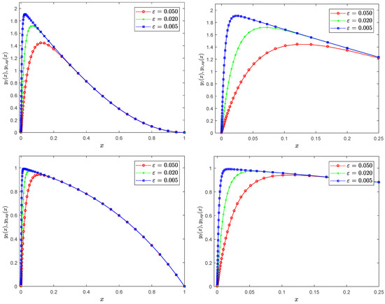
Figure 1. Exact solution (solid line) and approximate solution (dotted marked line) profiles of Example 1 at different values of $\epsilon$: (left) global region, (right) boundary region.

Figure 2 illustrates the distribution of the maximum pointwise error, denoted as ${‖\hspace{0.17em}\hspace{0.17em}.\hspace{0.17em}\hspace{0.17em}‖}_{\infty }=Error\left( x_{\omega }\right)={‖\hspace{0.17em}\hspace{0.17em}\overrightarrow{y}\left(x_{\omega }\right)-{ \overrightarrow{y}}_{ap}\left(x_{\omega }\right)\hspace{0.17em}\hspace{0.17em}‖}_{\infty }, x_{\omega }\in \left[a,b\right], \omega =0:K$, where $K$ represents a suitable number of grid points chosen for the purpose of comparison. The error is computed for the approximate solution (26) at various values of $\epsilon .$ The results depicted in Figure 2 demonstrate that as the perturbation parameter decreases, the accuracy of the approximate solution improves. Indeed, our results indicate that for $\epsilon \le 2^{-5},$ the maximum error in the approximate solution remains in the order $O\left({10}^{-15}\right)$.

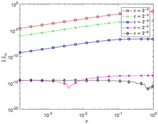
Figure 2. Maximum pointwise error for Example 1 with A-IRPSM at different values of $\epsilon$.

Table 1 presents the maximum error, denoted as $E_{max}={‖\hspace{0.17em}Error\left( x_{\omega }\right)\hspace{0.17em}\hspace{0.17em}‖}_{\infty }$, for both the A-RPSM and A-IRPSM in solving Example 1 at different values of ε and for $k=10$, while Table 2 presents the maximum error at $\epsilon ={10}^{-9}$ and for different values of $k$. The results from both tables confirm that as ε decreases, the accuracy of both methods increases, particularly when the first error term in (21) dominates due to larger $\epsilon$ values. Furthermore, the numerical results support the notion that increasing the number of series terms $k$ improves the accuracy of both methods, especially when the first error term is negligible, due to smaller $\epsilon$ values, and the second error term becomes dominant, highlighting a significant difference in accuracy between the RPSM and IRPSM, especially with increasing $k$. The results in Table 1 and Table 2 confirm that the A-IRPSM exhibits higher accuracy and demonstrates greater improvement in accuracy when compared to the A-RPSM.

Table 1. Numerical results with A-RPSM and A-IRPSM for Example 1 at $k=10$.

ε	Emax
	A-RPSM	A-IRPSM
$2^{-1}$	$2.6885\times {10}^{-1}$	$2.6885\times {10}^{-1}$
$2^{-2}$	$3.6571\times {10}^{-2}$	$3.6571\times {10}^{-2}$
$2^{-3}$	$6.7088\times {10}^{-4}$	$6.7088\times {10}^{-4}$
$2^{-4}$	$9.3072\times {10}^{-7}$	$2.2507\times {10}^{-7}$
$2^{-5}$	$9.3072\times {10}^{-7}$	$2.5616\times {10}^{-14}$
$2^{-6}$	$9.3072\times {10}^{-7}$	$3.5206\times {10}^{-15}$
$2^{-10}$	$9.3072\times {10}^{-7}$	$3.5250\times {10}^{-15}$
$2^{-20}$	$9.3072\times {10}^{-7}$	$3.5527\times {10}^{-15}$

Table 2. Numerical results with A-RPSM and A-IRPSM for Example 1 at $\epsilon ={10}^{-9}$.

k	Emax
	A-RPSM	A-IRPSM
$4$	$4.1665\times {10}^{-2}$	$5.2873\times {10}^{-3}$
$6$	$1.3888\times {10}^{-3}$	$1.1470\times {10}^{-11}$
8	$4.9468\times {10}^{-5}$	$3.5198\times {10}^{-15}$
10	$9.3555\times {10}^{-7}$	$3.5198\times {10}^{-15}$
12	$1.2641\times {10}^{-8}$	$3.5198\times {10}^{-15}$
14	$1.1470\times {10}^{-11}$	$3.5198\times {10}^{-15}$
16	$1.0518\times {10}^{-12}$	$3.5198\times {10}^{-15}$

Table 3 provides a comparison of the maximum error results for the A-RPSM, A-IRPSM and two other methods, namely a parameter-uniform finite difference method [32] and a spectral collocation method [24]. The comparison is conducted for the numerical results obtained in [24,32] at $\epsilon ={10}^{-8}$ and various numbers of grid points $N$, and the results of the A-RPSM and A-IRPSM at $k=10$. The results in Table 3 confirm that the A-IRPSM achieves significantly higher accuracy compared to the results of the A-RPSM and those presented in [24,32], even for the large number of grid points employed in [24,32] for accuracy improvement. This demonstrates the efficiency of the A-IRPSM in achieving accurate results with reduced computational effort.

Table 3. Maximum error $E_{max}$ in [24,32] and with A-RPSM and A-IRPSM for Example 1.

N	Uniform Finite Difference [32]	Collocation Method [24]	A-RPSM	A-IRPSM
128	$9.49 \times {10}^{-2}$	$1.85{ \times 10}^{-3}$	$9.31{ \times 10}^{-7}$	$3.5198 \times {10}^{-15}$
256	$5.76 \times {10}^{-2}$	$2.40{ \times 10}^{-6}$
512	$3.35 \times {10}^{-2}$	$5.47{ \times 10}^{-9}$
1024	$1.90 \times {10}^{-2}$	$5.41{ \times 10}^{-9}$

Example 2.

Consider the following SPBVS [13]

$$\left\{\begin{array}{c}\epsilon {y^{″}}_1\left(x\right)+{y^{\prime }}_1\left(x\right)-3y_1\left(x\right)+y_2\left(x\right)=-2 ,\\ \epsilon {y^{″}}_2\left(x\right)+{y^{\prime }}_2\left(x\right)+y_1\left(x\right)-3y_2\left(x\right)=-3 .\end{array}\right.$$

(27)

with boundary conditions

$$y_1(0)=y_1(1)=y_2(0)=y_2(1)=0$$

whose exact solution is given by

$$y_1(x)=\frac{9}{8}+\frac{5}{4}\left[\frac{e^{m_2}-1}{e^{m_1}-e^{m_2}}\right]e^{m_{1}x}+\frac{5}{4}\left[\frac{1-e^{m_1}}{e^{m_1}-e^{m_2}}\right]e^{m_{2}x}-\frac{1}{8}\left[\frac{e^{m_4}-1}{e^{m_3}-e^{m_4}}\right]e^{m_{3}x}-\frac{1}{8}\left[\frac{1-e^{m_3}}{e^{m_3}-e^{m_4}}\right]e^{m_{4}x},$$

and

$$y_2(x)\hspace{0.17em}=\frac{11}{8}+\frac{5}{4}\left[\frac{e^{m_2}-1}{ e^{m_1}-e^{m_2}}\right]e^{m_{1}x}+\frac{5}{4}\left[\frac{1-e^{m_1}}{ e^{m_1}-e^{m_2}}\right]e^{m_{2}x}\hspace{0.17em}-\frac{1}{8}\left[\frac{e^{m_4}-1}{e^{m_3}-e^{m_4}}\right]e^{m_{3}x}-\frac{1}{8}\left[\frac{1-e^{m_3}}{e^{m_3}-e^{m_4}}\right]e^{m_{4}x}\hspace{0.17em}\hspace{0.17em}.$$

where

$$m_1=(-1+\sqrt{1+8\epsilon })/2\epsilon , m_2=(-1-\sqrt{1+8\epsilon })/2\epsilon , m_3=(-1+\sqrt{1+ 16\epsilon })/2\epsilon ,\hspace{0.17em}\hspace{0.17em}{m}_4=(-1-\sqrt{1+8\epsilon })/2\epsilon \hspace{0.17em}.$$

The RTVS of (27) is given by

$$\left\{\begin{array}{c}{u^{\prime }}_1\left(x\right)-3u_1\left(x\right)+u_2\left(x\right)=-2 ,\\ {u^{\prime }}_2\left(x\right)+u_1\left(x\right)-3u_2\left(x\right)=-3 ,\\ u_1\left(1\right)=u_2\left(1\right)=0 . \end{array}\right.$$

(28)

When applying the RPSM with the 10th order to the RTVS (28), the result series solution is given by

$$\left\{\begin{array}{c}{u}_1^{10}=-2\left(x-1\right)-\frac{3}{2}{\left(x-1\right)}^2-\frac{1}{3}{\left(x-1\right)}^3+\frac{1}{2}{\left(x-1\right)}^4+\frac{11}{15}{\left(x-1\right)}^5+\frac{3}{5}{\left(x-1\right)}^6\\ +\frac{118}{315}{\left(x-1\right)}^7+\frac{41}{210}{\left(x-1\right)}^8+\frac{251}{2835}{\left(x-1\right)}^9+\frac{169}{4725}{\left(x-1\right)}^{10}+\mathrm{O}\left({\left(x-1\right)}^{11}\right) ,\\ u_2^{10}=-3\left(x-1\right)-\frac{7}{2}{\left(x-1\right)}^2-3{\left(x-1\right)}^3-\frac{13}{6}{\left(x-1\right)}^4-\frac{7}{5}{\left(x-1\right)}^5-\frac{37}{45}{\left(x-1\right)}^6\\ -\frac{46}{105}{\left(x-1\right)}^7-\frac{19}{90}{\left(x-1\right)}^8-\frac{29}{315}{\left(x-1\right)}^9-\frac{517}{14175}{\left(x-1\right)}^{10}+\mathrm{O}\left({\left(x-1\right)}^{11}\right) .\end{array}\right.$$

(29)

Applying the Laplace–Padé [5/5] algorithm to (29) results in

$$\left\{\begin{array}{c}{u}_{1,ap}=\frac{1}{8}{\mathrm{e}}^{4x-4}-\frac{5}{4}{\mathrm{e}}^{2x-2}+\frac{9}{8 } , \\ u_{2,ap}=-\frac{5}{4}{\mathrm{e}}^{2x-2}-\frac{1}{8}{\mathrm{e}}^{4x-4}+\frac{11}{8} .\end{array}\right.$$

(30)

Thus, we have an approximate analytical solution of the SPBVS (27), given by

$$\left\{\begin{array}{c}{y}_{1,ap}=\frac{1}{8}{\mathrm{e}}^{4x-4}-\frac{5}{4}{\mathrm{e}}^{2x-2}+\frac{9}{8}+\left(-\frac{1}{8}{\mathrm{e}}^{-4}+\frac{5}{4}{\mathrm{e}}^{-2}-\frac{9}{8}\right){\mathrm{e}}^{-\frac{x}{\epsilon }} ,\\ y_{2,ap}=-\frac{5}{4}{\mathrm{e}}^{2x-2}-\frac{1}{8}{\mathrm{e}}^{4x-4}+\frac{11}{8}+\left(\frac{1}{8}{\mathrm{e}}^{-4}+\frac{5}{4}{\mathrm{e}}^{-2}-\frac{11}{8}\right){\mathrm{e}}^{-\frac{x}{\epsilon }} .\end{array}\right.$$

(31)

Figure 3 presents the profiles of the exact solution (solid line) and the approximate solution (dotted marked line) in Example 2 over (left) the problem domain $\left[0, 1\right]$ and (right) a boundary layer region for different values of $\epsilon$. Figure 4 illustrates the distribution of the maximum pointwise error for the approximate solution (31) at various values of $\epsilon$.

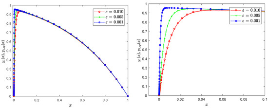
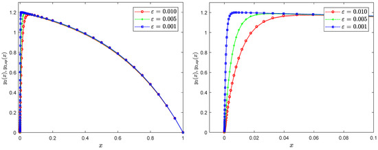
Figure 3. Exact solution (solid line) and approximate solution (dotted marked line) profiles of Example 2 at different values of ε: (left) global region, (right) boundary region.

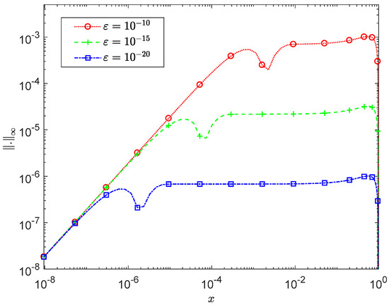
Figure 4. Maximum pointwise error for Example 2 with A-IRPSM at different values of ε.

The results in Figure 4 and Table 4 show that as the perturbation parameter decreases, the A-RPSM, A-IRPSM and the initial value method [13] exhibit an increase in accuracy. Furthermore, the accuracy of the A-IRPSM shows a greater improvement compared to the A-RPSM and the method in [13]. Indeed, similar results were obtained when comparing our results with the results presented in [13] for the remaining examples in that study.

Table 4. Maximum error, $E_{max}$, in [13] and with A-RPSM and A-IRPSM for Example 2.

ε	Initial Value Method [13]	A-RPSM	A-IRPSM
$2^{-1}$	$2.5466{ \times 10}^{-1}$	$1.4192{ \times 10}^{-1}$	$1.6288{ \times 10}^{-1}$
$2^{-3}$	$9.8552{ \times 10}^{-2}$	$8.9335{ \times 10}^{-2}$	$8.9453{ \times 10}^{-2}$
$2^{-5}$	$3.0295{ \times 10}^{-2}$	$3.0222{ \times 10}^{-2}$	$3.0261{ \times 10}^{-2}$
$2^{-7}$	$8.1371{ \times 10}^{-3}$	$1.1951{ \times 10}^{-2}$	$8.1045{ \times 10}^{-3}$
$2^{-9}$	$2.0972{ \times 10}^{-3}$	$1.0026{ \times 10}^{-2}$	$2.0647{ \times 10}^{-3}$
$2^{-11}$	$5.5161{ \times 10}^{-4}$	$9.9961{ \times 10}^{-3}$	$5.1865{ \times 10}^{-4}$
$2^{-13}$	$1.6232{ \times 10}^{-4}$	$9.9152{ \times 10}^{-3}$	$1.2982{ \times 10}^{-4}$
$2^{-15}$	$6.4966{ \times 10}^{-5}$	$9.8703{ \times 10}^{-3}$	$3.2465{ \times 10}^{-5}$
$2^{-17}$	$4.0617{ \times 10}^{-5}$	$9.8591{ \times 10}^{-3}$	$8.1169{ \times 10}^{-6}$
$2^{-19}$	$3.4529{ \times 10}^{-5}$	$9.8563{ \times 10}^{-3}$	$2.0293{ \times 10}^{-6}$
$2^{-21}$	$3.3007{ \times 10}^{-5}$	$9.8554{ \times 10}^{-3}$	$5.0732{ \times 10}^{-7}$
$2^{-23}$	$3.2625{ \times 10}^{-5}$	$9.8554{ \times 10}^{-3}$	$1.2683{ \times 10}^{-7}$

The results in Table 5 validate that increasing the value of $k$ leads to improved accuracy for both methods, with the A-IRPSM outperforming the A-RPSM in terms of higher accuracy and demonstrating a greater improvement in accuracy.

Table 5. Numerical results with A-RPSM and A-IRPSM for Example 2 at $\epsilon ={10}^{-9}$.

k	Emax
	A-RPSM	A-IRPSM
$4$	$8.7015{ \times 10}^{-1}$	$1.1797{ \times 10}^{-1}$
$6$	$2.9240{ \times 10}^{-1}$	$5.6345{ \times 10}^{-10}$
8	$6.5438{ \times 10}^{-2}$	$5.6345{ \times 10}^{-10}$
10	$9.8533{ \times 10}^{-3}$	$5.6345{ \times 10}^{-10}$
12	$1.0447{ \times 10}^{-3}$	$5.6345{ \times 10}^{-10}$
14	$8.1210{ \times 10}^{-5}$	$5.6345{ \times 10}^{-10}$
16	$4.4168{ \times 10}^{-6}$	$5.6345{ \times 10}^{-10}$

The present method can be extended to problems with specific Robin boundary conditions of the form $y_i\left(a\right)+\epsilon {\propto }_i{y^{\prime }}_i\left(a\right)={\alpha }_i$, $y_i\left(a\right)+\epsilon {\vartheta }_i{y^{\prime }}_i\left(a\right)={\alpha }_i$, $i=1,2,$ where ${\propto }_i$ and ${\mathsf{\vartheta }}_i$ are constants. To illustrate this, let us consider the following example.

Example 3.

Consider the following SPBVS [28]

$$\left\{\begin{array}{c}\epsilon {y^{″}}_1\left(x\right)+\left(2x+1\right){y^{\prime }}_1\left(x\right)-x^2{y^{\prime }}_2\left(x\right)+2y_1\left(x\right)-2x{y}_2\left(x\right)=\hspace{0.17em}\hspace{0.17em}{f}_1\left(x\right) ,\\ \epsilon {y^{″}}_2\left(x\right)-x^2{y^{\prime }}_1\left(x\right)+{y^{\prime }}_2\left(x\right)-2x{y}_1\left(x\right)\hspace{0.17em}\hspace{0.17em}\hspace{0.17em}\hspace{0.17em}=\hspace{0.17em}\hspace{0.17em}\hspace{0.17em}\hspace{0.17em}{f}_2\left(x\right) , \end{array}\right.$$

(32)

with Robin boundary conditions

$$\begin{array}{l}{y}_1(0)+\epsilon {y^{\prime }}_1(0)=1,\hspace{0.17em}\hspace{0.17em}\hspace{0.17em}\hspace{0.17em}\hspace{0.17em}\hspace{0.17em}\hspace{0.17em}{y}_1(1)+\epsilon {y^{\prime }}_1(1)=2+2\epsilon \hspace{0.17em},\hspace{0.17em}\\ y_2(0)+\epsilon {y^{\prime }}_2(0)=2,\hspace{0.17em}\hspace{0.17em}\hspace{0.17em}\hspace{0.17em}\hspace{0.17em}\hspace{0.17em}\hspace{0.17em}\hspace{0.17em}{y}_2(1)+\epsilon {y^{\prime }}_2(1)=4+3\epsilon -\epsilon \cos (1)-\sin (1)\hspace{0.17em},\hspace{0.17em}\end{array}$$

and where $f_1(x)$ and $f_2(x)$ are given by

$$\begin{array}{c}{f}_1\left(x\right)=\frac{\left(\left(-2+4x\right)\mathsf{\epsilon }+2x-2x^2\right){\mathrm{e}}^{-\frac{x}{\mathsf{\epsilon }}}}{\mathsf{\epsilon }}+2\mathsf{\epsilon }+2-4x^3+x^2\left(3+\mathrm{c}\mathrm{o}\mathrm{s}\left(x\right)\right)+2x\left(\sin \left(x\right)-1\right),\hfill \\ f_2\left(x\right)=-\frac{x\left(x-2\mathsf{\epsilon }\right){\mathrm{e}}^{-\frac{x}{\mathsf{\epsilon }}}}{\mathsf{\epsilon }}+2\mathsf{\epsilon }+\mathsf{\epsilon }s\mathrm{i}\mathrm{n}\left(x\right)-4x^3+1-\mathrm{c}\mathrm{o}\mathrm{s}\left(x\right).\hfill \end{array}$$

The exact solution of the SPBVS (32) is given by

$$\begin{array}{c}{y}_1\left(x\right)=1+x^2-e^{-\frac{x}{\epsilon }}\hspace{0.17em}\hspace{0.17em}, \hfill \\ y_2\left(x\right)=2+x\left(1+x\right)-\sin x-2e^{-\frac{x}{\epsilon }}\hspace{0.17em}\hspace{0.17em}.\hfill \end{array}$$

(33)

The RTVS of (32) is given by

$$\left\{\begin{array}{c}\left(2x+1\right){u^{\prime }}_1\left(x\right)-x^2{u^{\prime }}_2\left(x\right)+2u_1\left(x\right)-2x{u}_2\left(x\right)=2-2x \\ +3x^2-4x^3+x^2\cos \left(x\right)+2x\sin \left(x\right) ,\\ -x^2{u^{\prime }}_1\left(x\right)+{u^{\prime }}_2\left(x\right)-2x{u}_1\left(x\right)\hspace{0.17em}=\hspace{0.17em}1-4x^3-\mathit{cos}\left(x\right)\hspace{0.17em},\hfill \\ u_1\left(1\right)=2,\hspace{0.17em}\hspace{0.17em}\hspace{0.17em}{u}_2\left(1\right)=4-\sin \left(1\right)\hspace{0.17em}.\hspace{0.17em}\hfill \end{array}\right.$$

(34)

Applying the RPSM with the 10th order to the RTVS (34) results in

$$\left\{\begin{array}{c}{u}_1^{10}=x^2+1 , \\ { u}_2^{10}=\frac{61067}{19334}+\frac{79249}{32219}\left(x-1\right)+\frac{38904}{27383}{\left(x-1\right)}^2+\frac{8704}{96657}{\left(x-1\right)}^3-\frac{4236}{120817}{\left(x-1\right)}^4\\ -\frac{2176}{483285}{\left(x-1\right)}^5++\frac{706}{604085}{\left(x-1\right)}^6+\frac{1070}{9981079}{\left(x-1\right)}^7-\frac{375}{17968534}{\left(x-1\right)}^8\\ -\frac{130}{87311121}{\left(x-1\right)}^9+\frac{25}{107811204}{\left(x-1\right)}^{10}+\mathrm{O}\left({\left(x-1\right)}^{11}\right) .\\ \hspace{0.17em}\hspace{0.17em}\hspace{0.17em}\hspace{0.17em}\hspace{0.17em}\hspace{0.17em}\hspace{0.17em}\hspace{0.17em}\hspace{0.17em}\hspace{0.17em}\hspace{0.17em}\end{array}\right.$$

(35)

Applying the Laplace–Padé [5/5] algorithm to (35) results in

$$\left\{\begin{array}{c}{u}_{1,ap}=x^2+1 , \\ u_{2,ap}=2+x\left(1+x\right)-\frac{2069535434}{2459425781}\cos \left(x-1\right)-\frac{1114525615}{2062781526}\sin \left(x-1\right) .\hfill \end{array}\right.$$

Thus, we have an approximate analytical solution to the SPBVS (32), given by

$$\left\{\begin{array}{c}{y}_{1,ap}=1+x^2-e^{-\frac{x}{\epsilon }} , \hfill \\ y_{2,ap}=2+x\left(1+x\right)-\frac{2069535434}{2459425781}\cos \left(x-1\right)-\frac{1114525615}{2062781526}\sin \left(x-1\right)-2e^{-\frac{x}{\epsilon }} .\hfill \end{array}\right.$$

(36)

Figure 5 presents the profiles of the exact solution (solid line) and the approximate solution (dotted marked line) in Example 3 over (left) the problem domain $\left[0, 1\right]$ and (right) a boundary layer region for different values of $\epsilon$. Figure 6 illustrates the maximum pointwise error of the solution (36) across different values of $\epsilon$. Moreover, Table 6 presents the maximum error in Example 3 with the A-RPSM and A-IRPSM for different values of $\epsilon$ and at $k=10$. As mentioned in Section 3.3, and from (33) and (36), we note that the asymptotic approximation yields the exact solution of the boundary layer of problem (32). Consequently, the remaining error is unaffected by the perturbation parameter and is solely determined by the method employed to solve the RTVS.

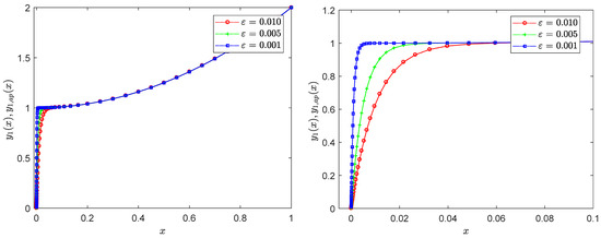
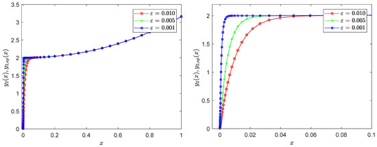
Figure 5. Exact solution (solid line) and approximate solution (dotted marked line) profiles of Example 3 at different values of ε: (left) global region, (right) boundary region.

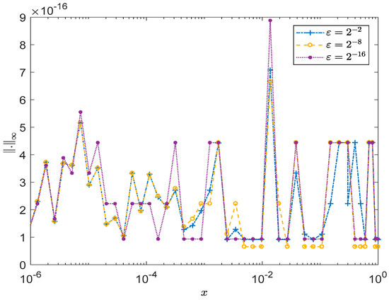
Figure 6. Maximum pointwise error for Example 3 with A-IRPSM at different values of ε.

Table 6. Maximum error, $E_{max}$, with A-RPSM and A-IRPSM for Example 3.

ε	A-RPSM	A-IRPSM
$2^{-1}$	$1.6845{ \times 10}^{-8}$	$6.6657{ \times 10}^{-15}$
$2^{-5}$	$1.6845{ \times 10}^{-8}$	$6.6613{ \times 10}^{-15}$
$2^{-10}$	$1.6845{ \times 10}^{-8}$	$6.6613{ \times 10}^{-15}$
$2^{-20}$	$1.6845{ \times 10}^{-8}$	$8.8818{ \times 10}^{-15}$

Notably, the maximum pointwise error in the approximate solution (36) remains in the order of $O({10}^{-15})$ even at $\epsilon =1$. Therefore, the obtained approximate solution serves as an exceptional representation of the exact solution.

The maximum error of the A-RPSM and A-IRPSM in solving Example 3 for different values of $k$ and at $\epsilon ={10}^{-9}$ is presented in Table 7. The results in Table 7 corroborate the results from Table 2 and Table 5, confirming that increasing the value of $k$ leads to enhanced accuracy for both methods. Additionally, the results validate that the A-IRPSM demonstrates a greater improvement in accuracy compared to the A-RPSM.

Table 7. Numerical results with A-RPSM and A-IRPSM for Example 3 at $\epsilon ={10}^{-9}$.

k	Emax
	A-RPSM	A-IRPSM
$4$	$5.5445{ \times 10}^{-3}$	$9.9663{ \times 10}^{-3}$
$6$	$1.2636{ \times 10}^{-4}$	$1.3804{ \times 10}^{-4}$
8	$1.7054{ \times 10}^{-6}$	$9.7456{ \times 10}^{-6}$
10	$1.5194{ \times 10}^{-8}$	$2.0000{ \times 10}^{-14}$
12	$9.5953{ \times 10}^{-11}$	$6.0000{ \times 10}^{-14}$
14	$4.5167{ \times 10}^{-13}$	$3.0000{ \times 10}^{-14}$
16	$1.6454{ \times 10}^{-15}$	$2.9952{ \times 10}^{-15}$

Example 4.

Consider the following SPBVS [34]

$$\left\{\begin{array}{c}\epsilon {y^{″}}_1\left(x\right)+{y^{\prime }}_1\left(x\right)-2y_1\left(x\right)+y_2\left(x\right)=-e^x \\ \epsilon {y^{″}}_2\left(x\right)+2{y^{\prime }}_2\left(x\right)+y_1\left(x\right)-4y_2\left(x\right)=-\cos x\end{array}\right.,$$

(37)

with boundary conditions

$$y_1(0)=y_1(1)=y_2(0)=y_2(1)=0$$

The exact solution of the SPBVS (37) is not unavailable.

The RTVS of (37) is given by

$$\left\{\begin{array}{c}{u^{\prime }}_1\left(x\right)-2u_1\left(x\right)+u_2\left(x\right)=-e^x , \hfill \\ \hspace{0.17em}2{u^{\prime }}_2\left(x\right)+{u^{\prime }}_1\left(x\right)-4u_2\left(x\right)=-cos\left(x\right),\hfill \\ u_1\left(1\right)=0,\hspace{0.17em}\hspace{0.17em}\hspace{0.17em}{u}_2\left(1\right)=0\hspace{0.17em}.\hfill \end{array}\right.$$

(38)

Applying the RPSM with the 10th order to the RTVS (38) results in

$$\left\{\begin{array}{c}{u}_1^{10}=-\frac{49171}{18089}x+\frac{49171}{18089}-\frac{44174}{11205}{\left(x-1\right)}^2-\frac{63719}{19380}{\left(x-1\right)}^3-\frac{38383}{18852}{\left(x-1\right)}^4-\frac{104319}{101549}{\left(x-1\right)}^5-\frac{20601}{46486}{\left(x-1\right)}^6 \\ \hspace{0.17em}\hspace{0.17em}\hspace{0.17em}\hspace{0.17em}\hspace{0.17em}\hspace{0.17em}\hspace{0.17em}\hspace{0.17em}\hspace{0.17em}\hspace{0.17em}\hspace{0.17em}-\frac{17861}{106840}{\left(x-1\right)}^7-\frac{5217}{93446}{\left(x-1\right)}^8-\frac{4063}{243619}{\left(x-1\right)}^9-\frac{1720}{382297}{\left(x-1\right)}^{10}+O{\left(x-1\right)}^{11}\hspace{0.17em}\hspace{0.17em}, \\ u_2^{10}=-\frac{8704}{32219}x+\frac{8704}{32219}\frac{55241}{89129}{\left(x-1\right)}^2+\frac{24913}{22338}{\left(x-1\right)}^3+\frac{29383}{30894}{\left(x-1\right)}^4+\frac{28998}{49843}{\left(x-1\right)}^5+\frac{8047}{28727}{\left(x-1\right)}^6 \\ \hspace{0.17em}\hspace{0.17em}\hspace{0.17em}\hspace{0.17em}\hspace{0.17em}\hspace{0.17em}\hspace{0.17em}\hspace{0.17em}\hspace{0.17em}\hspace{0.17em}\hspace{0.17em}+\frac{10245}{91684}{\left(x-1\right)}^7+\frac{9991}{260361}{\left(x-1\right)}^8+\frac{2162}{185925}{\left(x-1\right)}^9+\frac{1211}{383268}{\left(x-1\right)}^{10}+O{\left(x-1\right)}^{11}\hspace{0.17em}\hspace{0.17em}.\end{array}\right.$$

(39)

Applying the Laplace–Padé [5/5] algorithm to (39) results in

$$\left\{\begin{array}{l}{u}_{1,ap}=\left(-\frac{9473}{209200}\cos \left(\frac{126896}{126897}x-\frac{126896}{126897}\right)-\frac{5831}{60839}\sin \left(\frac{126896}{126897}x-\frac{126896}{126897}\right)\right){\mathrm{e}}^{-\frac{77}{27226394}x+\frac{77}{27226394}}\\ \hspace{0.17em}\hspace{0.17em}\hspace{0.17em}\hspace{0.17em}\hspace{0.17em}\hspace{0.17em}\hspace{0.17em}\hspace{0.17em}\hspace{0.17em}\hspace{0.17em}\hspace{0.17em}\hspace{0.17em}\hspace{0.17em}\hspace{0.17em}\hspace{0.17em}\hspace{0.17em}-\frac{15571}{3369}{\mathrm{e}}^{\frac{24760}{19151}x-\frac{24760}{19151}}-\frac{21873}{28414}{\mathrm{e}}^{\frac{66205}{24456}x-\frac{66205}{24456}}+\frac{28359}{5216}{\mathrm{e}}^{\frac{86476}{86475}x-\frac{86476}{86475}}\hspace{0.17em}\hspace{0.17em},\\ u_{2,ap}=\left(\frac{12563}{2382837}\cos \left(\frac{3278689}{3278688}x-\frac{3278689}{3278688}\right)-\frac{22754}{96023}\sin \left(\frac{3278689}{3278688}x-\frac{3278689}{3278688}\right)\right){\mathrm{e}}^{\frac{16}{48992101}x-\frac{16}{48992101}}\\ \hspace{0.17em}\hspace{0.17em}\hspace{0.17em}\hspace{0.17em}\hspace{0.17em}\hspace{0.17em}\hspace{0.17em}\hspace{0.17em}\hspace{0.17em}\hspace{0.17em}\hspace{0.17em}\hspace{0.17em}\hspace{0.17em}\hspace{0.17em}\hspace{0.17em}\hspace{0.17em}\hspace{0.17em}+\frac{5974}{10975}{\mathrm{e}}^{\frac{99229}{36655}x-\frac{99229}{36655}}-\frac{242455}{74193}{\mathrm{e}}^{\frac{16699}{12916}x-\frac{16699}{12916}}+\frac{45613}{16780}{\mathrm{e}}^{\frac{1795333}{1795332}x-\frac{1795333}{1795332}}\hspace{0.17em}\hspace{0.17em}\hspace{0.17em}.\end{array}\right.$$

(40)

Thus, we have an approximate analytical solution to the SPBVS (37), given by

$$\left\{\begin{array}{l}{y}_{1,ap}=\left(-\frac{9473}{209200}\cos \left(\frac{126896}{126897}x-\frac{126896}{126897}\right)-\frac{5831}{60839}\sin \left(\frac{126896}{126897}x-\frac{126896}{126897}\right)\right){\mathrm{e}}^{-\frac{77}{27226394}x+\frac{77}{27226394}}\\ \hspace{0.17em}\hspace{0.17em}\hspace{0.17em}\hspace{0.17em}\hspace{0.17em}\hspace{0.17em}\hspace{0.17em}\hspace{0.17em}\hspace{0.17em}\hspace{0.17em}\hspace{0.17em}\hspace{0.17em}\hspace{0.17em}\hspace{0.17em}\hspace{0.17em}\hspace{0.17em}-\frac{15571}{3369}{\mathrm{e}}^{\frac{24760}{19151}x-\frac{24760}{19151}}-\frac{21873}{28414}{\mathrm{e}}^{\frac{66205}{24456}x-\frac{66205}{24456}}+\frac{28359}{5216}{\mathrm{e}}^{\frac{86476}{86475}x-\frac{86476}{86475}}-\frac{7363274623}{10000000000}{\mathrm{e}}^{-\frac{x}{\epsilon }}\hspace{0.17em}\hspace{0.17em}\hspace{0.17em},\\ y_{2,ap}=\left(\frac{12563}{2382837}\cos \left(\frac{3278689}{3278688}x-\frac{3278689}{3278688}\right)-\frac{22754}{96023}\sin \left(\frac{3278689}{3278688}x-\frac{3278689}{3278688}\right)\right){\mathrm{e}}^{\frac{16}{48992101}x-\frac{16}{48992101}}\\ \hspace{0.17em}\hspace{0.17em}\hspace{0.17em}\hspace{0.17em}\hspace{0.17em}\hspace{0.17em}\hspace{0.17em}\hspace{0.17em}\hspace{0.17em}\hspace{0.17em}\hspace{0.17em}\hspace{0.17em}\hspace{0.17em}\hspace{0.17em}\hspace{0.17em}\hspace{0.17em}\hspace{0.17em}+\frac{5974}{10975}{\mathrm{e}}^{\frac{99229}{36655}x-\frac{99229}{36655}}-\frac{242455}{74193}{\mathrm{e}}^{\frac{16699}{12916}x-\frac{16699}{12916}}+\frac{45613}{16780}{\mathrm{e}}^{\frac{1795333}{1795332}x-\frac{1795333}{1795332}}-\frac{683232499}{2000000000}{\mathrm{e}}^{-\frac{2x}{\epsilon }}\hspace{0.17em}\hspace{0.17em}\hspace{0.17em}.\end{array}\right.$$

(41)

Due to the unavailability of the exact solution to the SPBVS (37), we adopted the numerical solution obtained using the bvp4c built-in function in MATLAB [63] with Abstol and Reltol values set to ${10}^{-10}$ as our reference solution for this test problem. To handle the challenges posed by steep gradients in the SPBVS, we augmented the bvp4c function with a continuation technique that allows for the solution of a BVP via a continuous transformation from an easier problem to the desired problem [64,65].

Figure 7 presents the profiles of the reference solution (solid line) and the approximate solution (dotted marked line) in Example 4 over (left) the problem domain $\left[0, 1\right]$ and (right) a boundary layer region for different values of $\epsilon$. Figure 8 illustrates the distribution of the maximum pointwise error for the approximate solution (41) at various values of $\epsilon$.

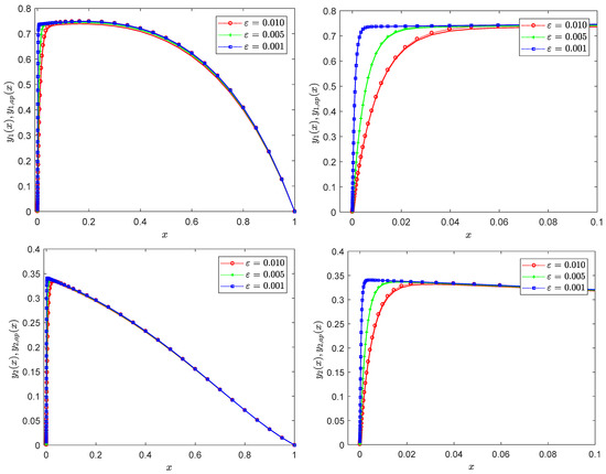
Figure 7. Exact solution (solid line) and approximate solution (dotted marked line) profiles of Example 4 at different values of ε: (left) global region, (right) boundary region.

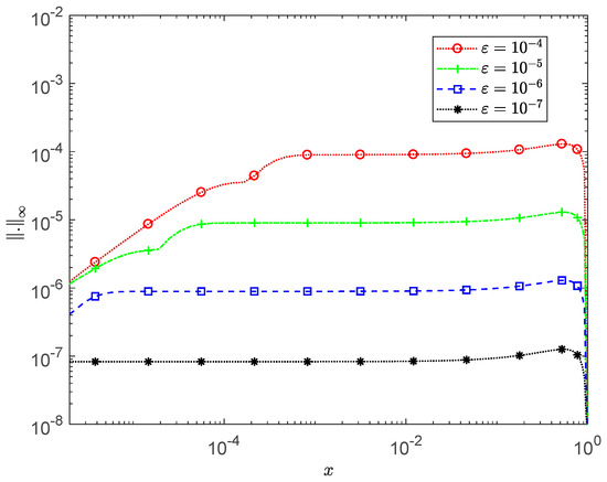
Figure 8. Maximum pointwise error for Example 4 with A-IRPSM at different values of ε.

The results in Table 8 corroborate the results from Table 2, Table 5 and Table 7, confirming that increasing the value of $k$ leads to enhanced accuracy for both methods. Additionally, the results validate that the A-IRPSM demonstrates a greater improvement in accuracy compared to the A-RPSM.

Table 8. Maximum error $E_{max}$ with A-RPSM and A-IRPSM for Example 4.

ε	A-RPSM	A-IRPSM
${10}^{-1}$	$9.6405{ \times 10}^{-2}$	$9.6406{ \times 10}^{-2}$
${10}^{-2}$	$1.2536{ \times 10}^{-2}$	$1.2536{ \times 10}^{-2}$
${10}^{-3}$	$1.2920{ \times 10}^{-3}$	$1.2922{ \times 10}^{-3}$
${10}^{-4}$	$8.9957{ \times 10}^{-4}$	$1.2962{ \times 10}^{-4}$
${10}^{-5}$	$8.9957{ \times 10}^{-4}$	$1.2963{ \times 10}^{-5}$
${10}^{-6}$	$8.9957{ \times 10}^{-4}$	$1.2932{ \times 10}^{-6}$
${10}^{-7}$	$8.9957{ \times 10}^{-4}$	$1.2620{ \times 10}^{-7}$

This method can be extended to higher dimensions of SPBVS, as demonstrated by the following three-dimensional example.

Example 5.

Consider the following system of the SPBVS [22,26,27]

$$\left\{\begin{array}{l}\epsilon {y^{″}}_1(x)+3{y^{\prime }}_1(x)-{y^{\prime }}_2(x)-{y^{\prime }}_3(x)=4\hspace{0.17em}\hspace{0.17em},\\ \epsilon {y^{″}}_2(x)-{y^{\prime }}_1(x)+4{y^{\prime }}_2(x)-2{y^{\prime }}_3(x)=-11\hspace{0.17em}\hspace{0.17em},\\ \epsilon {y^{″}}_3(x)-{y^{\prime }}_1(x)-2{y^{\prime }}_2(x)+4{y^{\prime }}_3(x)=7\hspace{0.17em}\hspace{0.17em},\end{array}\right.$$

(42)

with boundary conditions

$$\left\{\begin{array}{l}{y}_1(0)=-1,\hspace{0.17em}\hspace{0.17em}\hspace{0.17em}\hspace{0.17em}{y}_1(1)=e^{-1/\epsilon }-2e^{-4/\epsilon }+1\hspace{0.17em}\hspace{0.17em},\\ y_2(0)=4\hspace{0.17em}\hspace{0.17em},\hspace{0.17em}\hspace{0.17em}\hspace{0.17em}\hspace{0.17em}\hspace{0.17em}{y}_2(1)=e^{-1/\epsilon }+e^{-4/\epsilon }+2e^{-6/\epsilon }-2\hspace{0.17em}\hspace{0.17em},\\ y_3(0)=-1\hspace{0.17em}\hspace{0.17em},\hspace{0.17em}\hspace{0.17em}\hspace{0.17em}{y}_3(1)=e^{-1/\epsilon }+e^{-4/\epsilon }-2e^{-6/\epsilon }\hspace{0.17em}\hspace{0.17em}.\end{array}\right.$$

The exact solution of the SPBVS (42) is given by

$$\left\{\begin{array}{l}{y}_1=x+e^{-x/\epsilon }-2e^{-4x/\epsilon }\hspace{0.17em}\hspace{0.17em},\\ y_2=-2x+e^{-x/\epsilon }+e^{-4x/\epsilon }+2e^{-6x/\epsilon }\hspace{0.17em}\hspace{0.17em},\\ y_3=x-1+e^{-x/\epsilon }+e^{-4x/\epsilon }-2e^{-6x/\epsilon }\hspace{0.17em}\hspace{0.17em}.\end{array}\right.$$

(43)

The RTVS of (42) is obtained by setting$\epsilon =0$ in (42) and given by

$$\left\{\begin{array}{l}3{u^{\prime }}_1(x)-{u^{\prime }}_2(x)-{u^{\prime }}_3(x)=4\hspace{0.17em}\hspace{0.17em},\\ -{u^{\prime }}_1(x)+4{u^{\prime }}_2(x)-2{u^{\prime }}_3(x)=-11\hspace{0.17em}\hspace{0.17em},\\ -{u^{\prime }}_1(x)-2{u^{\prime }}_2(x)+4{u^{\prime }}_3(x)=7\hspace{0.17em}\hspace{0.17em},\\ u_1(1)=1,\hspace{0.17em}\hspace{0.17em}{u}_1(1)=-2,\hspace{0.17em}\hspace{0.17em}{u}_1(1)=0.\end{array}\right.$$

(44)

Applying the RPSM with the 6th order to the RTVS (44) results in

$$\left\{\begin{array}{c}{u}_1^6=x , \\ u_2^6=-2x ,\\ u_3^6=x-1 .\end{array}\right.$$

(45)

And consequently, the result of the Laplace–Padé [5/5] algorithm is

$$\left.\begin{array}{c}{u}_{1,ap}=x , \\ u_{2,ap}=-2x ,\\ u_{3,ap}=x-1 .\end{array}\right\}.$$

(46)

Using the same procedure presented in Section 2.1, the boundary layer correction problem of the SPBVS (42) can be easily obtained and have a similar form to that presented in Equation (8) and for $i=1, 2, 3$. The resulting boundary layer correction problem is given by

$$\left\{\begin{array}{l}{\dot{v}}_1(t)+3v_1(t)-v_2(t)-v_3(t)=O(\epsilon ),\hspace{0.17em}\hspace{0.17em}{v}_1(0)=-1-u_{1,ap}(0)\hspace{0.17em}\hspace{0.17em},\\ {\dot{v}}_2(t)-v_1(t)+4v_2(t)-2v_3(t)=O(\epsilon ),\hspace{0.17em}\hspace{0.17em}\hspace{0.17em}{v}_2(0)=4-u_{2,ap}(0)\hspace{0.17em}\hspace{0.17em},\\ {\dot{v}}_3(t)-v_1(t)-2v_2(t)+4v_3(t)=O(\epsilon ),\hspace{0.17em}\hspace{0.17em}\hspace{0.17em}\hspace{0.17em}{v}_3(0)=-1-u_{3,ap}(0)\hspace{0.17em}\hspace{0.17em},\end{array}\right.$$

(47)

Problem (47) is a linear system of differential equations with constant coefficients that has an exact solution given by

$$\left\{\begin{array}{l}{v}_1(t)={\mathrm{e}}^{-t}-2{\mathrm{e}}^{-4t}\hspace{0.17em}+O(\epsilon )\hspace{0.17em},\\ v_2(t)={\mathrm{e}}^{-t}+{\mathrm{e}}^{-4t}+2{\mathrm{e}}^{-6t}+O(\epsilon )\hspace{0.17em}\hspace{0.17em},\\ v_3(t)={\mathrm{e}}^{-t}+{\mathrm{e}}^{-4t}-2{\mathrm{e}}^{-6t}\hspace{0.17em}+O(\epsilon )\hspace{0.17em}.\end{array}\right.$$

(48)

From the reduced solution (46) and the boundary layer solution (48), after replacing t with $\frac{x}{\epsilon }$ in (48), we have

$$\left\{\begin{array}{l}{y}_{1,ap}=x+e^{-x/\epsilon }-2e^{-4x/\epsilon }\hspace{0.17em}\hspace{0.17em},\\ y_{2,ap}=-2x+e^{-x/\epsilon }+e^{-4x/\epsilon }+2e^{-6x/\epsilon }\hspace{0.17em}\hspace{0.17em},\\ y_{3,ap}=x-1+e^{-x/\epsilon }+e^{-4x/\epsilon }-2e^{-6x/\epsilon }\hspace{0.17em}\hspace{0.17em}.\end{array}\right.$$

(49)

which is the exact solution (43) to the SPBVS (42).

For this example, as the solution of the RTVS (44) is a polynomial, both the A-RPSM and A-IRPSM methods yield the exact same polynomial solution. Consequently, these methods produce the same approximate solution (49) for the given problem (42).

Figure 9 shows the solution profile of Example 5 over (left) the problem domain $\left[0, 1\right]$ and (right) a boundary layer region for different values of $\epsilon$.

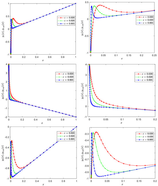
Figure 9. Exact solution (solid line) and approximate solution (dotted marked line) profiles of Example 5 at different values of ε: (left) global region, (right) boundary region.

5. Conclusions

In this paper, an efficient method for solving strongly coupled singularly perturbed convection–diffusion systems is presented. This method utilizes the reduced terminal value system and the boundary layer system, which has a known exact solution, to derive an approximate analytical solution for the original system. These systems have practical applications, and an approximate analytical solution is needed to gain insights into their behavior and analyze practical scenarios considering different physical parameters. The proposed method combines the RPSM, Padé approximation and Laplace transformation, resulting in a more accurate solution compared to traditional RPSM. The accuracy of the method is validated through error estimates, illustrative examples and comparisons with the existing literature. The numerical results demonstrate that decreasing the perturbation parameter or increasing the number of considered series terms improves the accuracy of this method, in agreement with the theoretical results presented in this paper. Furthermore, the A-IRPSM exhibits higher accuracy and greater improvement compared to the A-RPSM and other methods discussed in the literature. This method also demonstrates its reliability by yielding exact solutions for specific solved examples, highlighting its accuracy and trustworthiness. Additionally, the capability of extending this method to higher-dimensional singularly perturbed convection–diffusion systems is demonstrated through a three-dimensional test problem. The results clearly indicate the high accuracy of the method and its ability to provide continuous approximate or exact solutions for such systems. Future work will focus on extending this method to nonlinear problems and other types of singularly perturbed systems.

References

- Kokotović, P.V. Applications of singular perturbation techniques to control problems. SIAM Rev. 1984, 26, 501–550. [Google Scholar] [CrossRef]
- Thomas, G.P. Towards an improved turbulence model for wave-current interactions. In Second Annual Report to EU MAST-III Project “The Kinematics and Dynamics of Wave-Current Interactions”; Springer: Berlin/Heidelberg, Germany, 1998. [Google Scholar]
- Shishkin, G.I. Mesh approximation of singularly perturbed boundary-value problems for systems of elliptic and parabolic equations. Comput. Math. Math. Phys. 1995, 35, 429–446. [Google Scholar]
- Hsieh, P.-W.; Shih, Y.; Yang, S.-Y. A tailored finite point method for solving steady MHD duct flow problems with boundary layers. Commun. Comput. Phys. 2011, 10, 161–182. [Google Scholar] [CrossRef]
- El-Zahar, E.R.; Rashad, A.M.; Al-Juaydi, H.S. Studying massive suction impact on magneto-flow of a hybridized Casson nanofluid on a porous continuous moving or fixed surface. Symmetry 2022, 14, 627. [Google Scholar] [CrossRef]
- O’Malley, R. Introduction to Singular Perturbations; Academic Press: Cambridge, MA, USA, 1974. [Google Scholar]
- Miller, J.J.; O’Riordan, E.; Shishkin, G. Fitted Numerical Methods for Singular Perturbation Problems; World Scientific: London, UK, 1996. [Google Scholar]
- Roos, H.-G.; Stynes, M.; Tobiska, L. Robust Numerical Methods for Singularly Perturbed Differential Equations; Springer: Berlin/Heidelberg, Germany, 2008. [Google Scholar]
- Shanthi, V.; Ramanujam, N. Asymptotic numerical method for boundary value problems for singularly perturbed fourth-order ordinary differential equations with a weak interior layer. Appl. Math. Comput. 2006, 172, 252–266. [Google Scholar] [CrossRef]
- El-Zahar, E.R.; El-Kabeir, S.M. A new method for solving singularly perturbed boundary value problems. Appl. Math. Inf. Sci. 2013, 7, 927. [Google Scholar] [CrossRef]
- El-Zahar, E.R. Approximate analytical solutions of singularly perturbed fourth order boundary value problems using differential transform method. J. King Saud Univ.-Sci. 2013, 25, 257–265. [Google Scholar] [CrossRef]
- El-Zahar, E.R. Piecewise approximate analytical solutions of high-order singular perturbation problems with a discontinuous source term. Int. J. Differ. Equ. 2016, 2016, 1015634. [Google Scholar] [CrossRef]
- Valanarasu, T.; Ramanujam, N. Asymptotic initial-value method for a system of singularly perturbed second-order ordinary differential equations of convection-diffusion type. Int. J. Comput. Math. 2004, 81, 1381–1393. [Google Scholar] [CrossRef]
- Liu, C.S.; El-Zahar, E.R.; Chang, C.W. Higher-order asymptotic numerical solutions for singularly perturbed problems with variable coefficients. Mathematics 2022, 10, 2791. [Google Scholar] [CrossRef]
- Melesse, W.G.; Tiruneh, A.A.; Derese, G.A. Solving systems of singularly perturbed convection diffusion problems via initial value method. J. Appl. Math. 2020, 2020, 1062025. [Google Scholar] [CrossRef]
- Singh, G.; Natesan, S. A uniformly convergent numerical scheme for a coupled system of singularly perturbed reaction-diffusion equations. Numer. Funct. Anal. Optim. 2020, 41, 1172–1189. [Google Scholar] [CrossRef]
- Clavero, C.; Gracia, J.L.; Lisbona, F.J. An almost third order finite difference scheme for singularly perturbed reaction-diffusion system. J. Comput. Appl. Math. 2010, 234, 2501–2515. [Google Scholar] [CrossRef]
- Linss, T.; Madden, N. Layer-adapted meshes for a linear system of coupled singularly perturbed reaction-diffusion problems. IMA J. Numer. Anal. 2009, 29, 109–125. [Google Scholar] [CrossRef]
- Paramasivam, M.; Valarmathi, S.; Miller, J.J.H. Second-order parameter-uniform convergence for a finite difference method for a singularly perturbed linear reaction-diffusion system. Math. Commun. 2010, 15, 587–612. [Google Scholar]
- Das, P.; Natesan, S. A uniformly convergent hybrid scheme for singularly perturbed system of reaction-diffusion Robin type boundary-value problems. J. Appl. Math. Comput. 2013, 41, 447–471. [Google Scholar] [CrossRef]
- Madden, N.; Stynes, M. A uniformly convergent numerical method for a coupled system of singularly perturbed linear reaction-diffusion problems. IMA J. Numer. Anal. 2003, 23, 627–644. [Google Scholar] [CrossRef]
- O’Riordan, E.; Stynes, J.; Stynes, M. An iterative numerical algorithm for a strongly coupled system of singularly perturbed convection-diffusion problems. In International Conference on Numerical Analysis and Its Applications; Springer: Berlin/Heidelberg, Germany, 2008; pp. 104–115. [Google Scholar] [CrossRef]
- O’Riordan, E.; Stynes, M. Numerical analysis of a strongly coupled system of two singularly perturbed convection–diffusion problems. Adv. Comput. Math. 2009, 30, 101–121. [Google Scholar] [CrossRef]
- Sharp, N.; Trummer, M. A spectral collocation method for systems of singularly perturbed boundary value problems. Procedia Comput. Sci. 2017, 108, 725–734. [Google Scholar] [CrossRef]
- Hsieh, P.W.; Yang, S.Y.; You, C.S. A robust finite difference scheme for strongly coupled systems of singularly perturbed convection-diffusion equations. Numer. Methods Partial. Differ. Equ. 2018, 34, 121–144. [Google Scholar] [CrossRef]
- Yang, L. Rational spectral collocation combined with the singularity separated method for a system of singularly perturbed boundary value problems. Math. Probl. Eng. 2019, 2019, 9030565. [Google Scholar] [CrossRef]
- Chen, S.; Wang, Y.; Wu, X. Rational spectral collocation method for a coupled system of singularly perturbed boundary value problems. J. Comput. Math. 2011, 29, 458–473. [Google Scholar] [CrossRef]
- Liu, L.B.; Liang, Y.; Bao, X.; Fang, H. An efficient adaptive grid method for a system of singularly perturbed convection-diffusion problems with Robin boundary conditions. Adv. Differ. Equ. 2021, 2021, 6. [Google Scholar] [CrossRef]
- Roos, H.G. Special features of strongly coupled systems of convection-diffusion equations with two small parameters. Appl. Math. Lett. 2012, 25, 1127–1130. [Google Scholar] [CrossRef]
- Roos, H.G.; Reibiger, C. Analysis of a strongly coupled system of two convection-diffusion equations with full layer interaction. ZAMM-J. Appl. Math. Mech. Z. Angew. Math. Mech. 2011, 91, 537–543. [Google Scholar] [CrossRef]
- Linss, T. Analysis of a system of singularly perturbed convection-diffusion equations with strong coupling. SIAM J. Numer. Anal. 2009, 47, 1847–1862. [Google Scholar] [CrossRef]
- Cen, Z. Parameter-uniform finite difference scheme for a system of coupled singularly perturbed convection-diffusion equations. Int. J. Comput. Math. 2005, 82, 177–192. [Google Scholar] [CrossRef]
- Das, P.; Natesan, S. Numerical solution of a system of singularly perturbed convection-diffusion boundary value problems using mesh equidistribution technique. Aust. J. Math. Anal. Appl. 2013, 10, 1–17. [Google Scholar]
- Lin, T. Analysis of an upwind finite-difference scheme for a system of coupled singularly perturbed convection-diffusion equations. Computing 2007, 79, 23–32. [Google Scholar]
- Lorenz, J. Stability and monotonicity properties of stiff quasilinear boundary problems. Univ. Novom Sadu Zb. Rad. Prir.-Mat. Fak. Sec. Mat. 1982, 12, 151–175. [Google Scholar]
- Vulanovic, R. A uniform numerical method for quasilinear singular perturbation problems without turning points. Computing 1989, 41, 97–106. [Google Scholar] [CrossRef]
- El-Zahar, E.; El-Kabeir, S. Approximate Analytical Solution of Nonlinear Third-Order Singularly Perturbed BVPs Using Homotopy Analysis Method-Padé Method. J. Comput. Theor. Nanosci. 2016, 13, 8917–8927. [Google Scholar] [CrossRef]
- Naik, P.A.; Zu, J.; Ghoreishi, M. Estimating the approximate analytical solution of HIV viral dynamic model by using homotopy analysis method. Chaos Solitons Fractals 2020, 131, 109500. [Google Scholar] [CrossRef]
- Masjedi, P.K.; Weaver, P.M. Analytical solution for arbitrary large deflection of geometrically exact beams using the homotopy analysis method. Appl. Math. Model. 2022, 103, 516–542. [Google Scholar] [CrossRef]
- You, X.; Cui, J. Spherical Hybrid Nanoparticles for Homann Stagnation-Point Flow in Porous Media via Homotopy Analysis Method. Nanomaterials 2023, 13, 1000. [Google Scholar] [CrossRef] [PubMed]
- Alam, M.S.; Sharif, N.; Molla, M.H.U. Combination of modified Lindstedt-Poincare and homotopy perturbation methods. J. Low Freq. Noise Vib. Act. Control 2023, 42, 642–653. [Google Scholar] [CrossRef]
- Aljahdaly, N.H.; Alweldi, A.M. On the modified Laplace homotopy perturbation method for solving damped modified Kawahara equation and its application in a fluid. Symmetry 2023, 15, 394. [Google Scholar] [CrossRef]
- Moosavi Noori, S.R.; Taghizadeh, N. Modified differential transform method for solving linear and nonlinear pantograph type of differential and Volterra integro-differential equations with proportional delays. Adv. Differ. Equ. 2020, 2020, 649. [Google Scholar] [CrossRef]
- Benhammouda, B.; Vazquez-Leal, H.; Sarmiento-Reyes, A. Modified reduced differential transform method for partial differential-algebraic equations. J. Appl. Math. 2014, 2014, 279481. [Google Scholar] [CrossRef]
- Wang, F.; Kumar, R.V.; Sowmya, G.; El-Zahar, E.R.; Prasannakumara, B.C.; Khan, M.I.; Khan, S.U.; Malik, M.Y.; Xia, W.F. LSM and DTM-Padé approximation for the combined impacts of convective and radiative heat transfer on an inclined porous longitudinal fin. Case Stud. Therm. Eng. 2022, 35, 101846. [Google Scholar] [CrossRef]
- Benhammouda, B.; Vazquez-Leal, H.; Hernandez-Martinez, L. Modified differential transform method for solving the model of pollution for a system of lakes. Discret. Dyn. Nat. Soc. 2014, 2014, 645726. [Google Scholar] [CrossRef]
- Qayyum, M.; Fatima, Q.; Sohail, M.; El-Zahar, E.R.; Gokul, K.C. Extended residual power series algorithm for boundary value problems. Math. Probl. Eng. 2022, 2022, 1039222. [Google Scholar] [CrossRef]
- Ebaid, A.E. A reliable aftertreatment for improving the differential transformation method and its application to nonlinear oscillators with fractional nonlinearities. Commun. Nonlinear Sci. Numer. Simul. 2011, 16, 528–536. [Google Scholar] [CrossRef]
- Mohammed, H.A.-S. Solving initial value problems by residual power series method. Theor. Math. Appl. 2013, 3, 199–210. [Google Scholar]
- Abu Arqub, O.; El-Ajou, A.; Bataineh, A.S.; Hashim, I. A representation of the exact solution of generalized Lane-Emden equations using a new analytical method. In Abstract and Applied Analysis; Massimo, F., Ed.; Hindawi: New York, NY, USA, 2013; Volume 2013. [Google Scholar] [CrossRef]
- Momani, S.; Arqub, O.A.; Hammad, M.A.; Hammour, Z.A. A residual power series technique for solving systems of initial value problems. Appl. Math. Inf. Sci. 2016, 10, 765–775. [Google Scholar] [CrossRef]
- Alaroud, M. Application of Laplace residual power series method for approximate solutions of fractional IVP’s. Alex. Eng. J. 2022, 61, 1585–1595. [Google Scholar] [CrossRef]
- Dawar, A.; Khan, H.; Islam, S.; Khan, W. The improved residual power series method for a system of differential equations: A new semi-numerical method. Int. J. Model. Simul. 2023, 43, 1–14. [Google Scholar] [CrossRef]
- Fang, J.; Nadeem, M.; Islam, A.; Iambor, L.F. Modified residual power series approach for the computational results of Newell-Whitehead-Segel model with fractal derivatives. Alex. Eng. J. 2023, 77, 503–512. [Google Scholar] [CrossRef]
- Khan, H.; Ullah, I.; Ali, J.; Jamshed, W.; Aziz, A.; Irfan Shah, S. The solution of twelfth order boundary value problems by the improved residual power series method: New approach. Int. J. Model. Simul. 2023, 43, 64–74. [Google Scholar] [CrossRef]
- Chen, F.; Liu, Q.Q. Adomian decomposition method combined with Padé approximation and Laplace transform for solving a model of HIV infection of CD4+ T cells. Discret. Dyn. Nat. Soc. 2015, 2015, 584787. [Google Scholar] [CrossRef]
- Baker, G.A. Essentials of Padé Approximations; Academic Express: London, UK, 1975. [Google Scholar]
- Boyd, J.P. Padé approximant algorithm for solving nonlinear ordinary differential equation boundary value problems on an unbounded domain. Comput. Phys. 1997, 11, 299–303. [Google Scholar] [CrossRef]
- Yamada, H.S.; Ikeda, K.S. A numerical test of Padé approximation for some functions with singularity. Int. J. Comput. Math. 2014, 2014, 587430. [Google Scholar] [CrossRef]
- Vyatchin, A.V. On convergence of Padé approximants. Mosc. Univ. Math. Bull. 1982, 37, 1–4. [Google Scholar]
- Liu, L.B.; Chen, Y. A-posteriori error estimation in maximum norm for a strongly coupled system of two singularly perturbed convection–diffusion problems. J. Comput. Appl. Math. 2017, 313, 152–167. [Google Scholar] [CrossRef]
- Amir, M.; Ali, Q.; Raza, A.; Almusawa, M.Y.; Hamali, W.; Ali, A.H. Computational results of convective heat transfer for fractionalized Brinkman type tri-hybrid nanofluid with ramped temperature and non-local kernel. Ain Shams Eng. J. 2024, 15, 102576. [Google Scholar] [CrossRef]
- Shampine, L.F.; Kierzenka, J.; Reichelt, M.W. Solving boundary value problems for ordinary differential equations in MATLAB with bvp4c. Tutor. Notes 2000, 2000, 1–27. [Google Scholar]
- Cash, J.R.; Moore, G.; Wright, R.W. An automatic continuation strategy for the solution of singularly perturbed nonlinear boundary value problems. ACM Trans. Math. Softw. (TOMS) 2001, 27, 245–266. [Google Scholar] [CrossRef]
- Ascher, U.M.; Petzold, L.R. Computer Methods for Ordinary Differential Equations and Differential-Algebraic Equations; SIAM: Philadelphia, PA, USA, 1998; Volume 61. [Google Scholar] [CrossRef]
Disclaimer/Publisher’s Note: The statements, opinions and data contained in all publications are solely those of the individual author(s) and contributor(s) and not of MDPI and/or the editor(s). MDPI and/or the editor(s) disclaim responsibility for any injury to people or property resulting from any ideas, methods, instructions or products referred to in the content. |
© 2024 by the authors. Licensee MDPI, Basel, Switzerland. This article is an open access article distributed under the terms and conditions of the Creative Commons Attribution (CC BY) license (https://creativecommons.org/licenses/by/4.0/).