Modified Block Bootstrap Testing for Persistence Change in Infinite Variance Observations

Abstract

This paper investigates the properties of the change in persistence detection for observations with infinite variance. The innovations are assumed to be in the domain of attraction of a stable law with index $\kappa \in (0,2]$. We provide a new test statistic and show that its asymptotic distribution under the null hypothesis of non-stationary $I\left(1\right)$ series is a functional of a stable process. When the change point in persistence is not known, the consistency is always given under the alternative, either from stationary $I\left(0\right)$ to non-stationary $I\left(1\right)$ or vice versa. The proposed tests can be used to identify the direction of change and do not over-reject against constant $I\left(0\right)$ series, even in relatively small samples. Furthermore, we also consider the change point estimator which is consistent and the asymptotic behavior of the test statistic in the case of near-integrated time series. A block bootstrap method is suggested to determine critical values because the null asymptotic distribution contains the unknown tail index, which results in critical values depending on it. The simulation study demonstrates that the block bootstrap-based test is robust against change in persistence for heavy-tailed series with infinite variance. Finally, we apply our methods to the two series of the US inflation rate and USD/CNY exchange rate, and find significant evidence for persistence changes, respectively, from $I\left(0\right)$ to $I\left(1\right)$ and from $I\left(1\right)$ to $I\left(0\right)$.

1. Introduction

There is growing evidence to show that the parameters of autoregressive models fitted to many economic, financial and hydrology time series are not fixed across time; see, Busetti [1], Chen [2] and Belaire [3]. Being able to correctly characterize a time series into its separate stationary $I\left(0\right)$ and non-stationary $I\left(1\right)$ components has important implications for effective model building and accurate forecasting in economics and finance, especially concerning government budget deficits and inflation rates (e.g., Sibbertsen [4]). A number of testing procedures were proposed depending on whether the initial regime is $I\left(1\right)$ or $I\left(0\right)$. Kim [5] proposed regression-based ratio tests of the constant $I\left(0\right)$ null against the alternative of a single change in persistence, either from $I\left(0\right)$ to $I\left(1\right)$ or vice versa. Leybourne [6] discussed testing for the null hypothesis that the series is $I\left(1\right)$ throughout the sample versus the alternative that it switches from $I\left(1\right)$ to $I\left(0\right)$ and vice versa. When the direction of change is unknown, Leybourne [7] considered standardized cumulative sums of squared subsample residuals that are used to identify the direction of change and do not spuriously reject when the series is a constant $I\left(0\right)$ process. Since then, there have been further studies on the persistence change. For example, Cerqueti [8] presented panel stationary tests against changes in persistence, and Kejriwal [9] provided a bootstrap test for multiple persistence changes in a heteroskedastic time series. For more research on persistence change, we refer to Jin [10], Jin [11], Wingert [12], and Grote [13].

The above tests are designed to detect a change in persistence with finite variance and do not consider heavy-tailed series with infinite variance. However, Mittnik [14] argued that many types of data on economics and finance have a heavy tail character. It is of greater practical significance to test for the change point with heavy-tailed observations. Therefore, many scholars have paid more attention to the detection of change in persistence under heavy-tailed time series models. In the case of the $I\left(0\right)$ process null hypothesis, Han [15] used the ratio test statistic to consider the change-point detection with heavy-tailed innovations and proved its consistency as there is a persistence change presence. For the problem of the null hypothesis of the $I\left(1\right)$ process and the alternative hypothesis involving a change in persistence switching from $I\left(1\right)$ to $I\left(0\right)$, Qin [16] applied a Dickey–Fuller-type ratio test statistic to study for infinite variance observations. Related to online monitoring issues, Chen [17] adopted a kernel-weighted quasi-variance test to monitor the persistence change in heavy-tailed series. For more persistence change estimation and detection in heavy-tailed sequences with infinite variance, see Yang [18], Jin [19], Jin [20], and Wang [21].

However, the existing test methods on heavy-tailed sequences consider the tail index just belonging to $\kappa \in (1,2]$, without $\kappa \in (0,1]$, and suppose beforehand that the direction of persistence change is known. In this paper, we propose a new test statistic to test the null hypothesis $I\left(1\right)$ against the alternative of a change in persistence, either $I\left(0\right)\to I\left(1\right)$ or $I\left(1\right)\to I\left(0\right)$. The innovations are assumed to be stationary time series with heavy-tailed univariate marginal distributions, which are in the domain of attraction of $\kappa$-stable law with $\kappa \in (0,2]$. We take into account two types of time series models, a pure AR(1) model and a AR(1) model with a constant or a constant plus linear time trend. Recently, the asymptotic inference for a least squares (LS) estimate when the autoregressive parameter is close to 1 (i.e., the series is nearly non-stationary) has been receiving considerable attention in the statistics and econometric literature, such as Chan [22] and Cheng [23]. Therefore, we are also interested in deriving the asymptotic behavior of the proposed test in the context of the near-unit root. Since the critical values of asymptotic distribution depend on the unknown tail index $\kappa$. To solve this problem, a block bootstrap approximation method suggested by Paparoditis [24] is used to determine the critical values, and then its validity is proved. The performance of the bootstrap-based test in small samples is evaluated via an extensive Monte Carlo study. Finally, the feasibility of our proposed test procedures is illustrated through empirical analysis.

Although the main results of this paper bear some formal analogy with Leybourne [7], it offers a number of important new implications. First, it extends the work of persistence change detection with heavy-tailed sequences to the case wherein the innovation process is in the domain of attraction of a stable law with index $\kappa \in (0,2]$. Thus, we can perform the examination of structural change in persistence even if the mean of real data does not exist. Second, under the circumstances of infinite variance, both for non-stationary and nearly non-stationary series, the order of $({\widehat{\rho }}_{{}_T}-{\rho }_{{}_T})$ is T. This is somewhat intriguing as this order was originally motivated by the consideration of the magnitude of the observed Fisher’s information number in the finite variance case, as can be seen in Chan [25]. Third, as we all know, Kim [5] proved the ratio type test statistic diverges at the rate of $O_p\left(T^2\right)$, but it only can apply to the alternative hypothesis involving a persistence change, $I\left(0\right)\to I\left(1\right)$. The Dickey–Fuller type ratio test proposed by Leybourne [26] correctly rejects the null of no persistence change, and the tail in which the rejection occurs can also be used to identify the direction of change. The deficiency cannot be ignored since the divergence rate is less than $O_p\left(T\right)$. However, it is satisfying that the divergence rate of our proposed test statistic can reach $O_p\left(T^2\right)$. In addition, we do not need to assume that the direction of any possible change is known and the test almost never rejects in the left (right) tail when there is a change from $I\left(1\right)$ to $I\left(0\right)$ [$I\left(0\right)$–$I\left(1\right)$].

This paper is organized as follows. Section 2 introduces the model, some necessary assumptions, and the test statistic. Section 3 details the large sample properties of the tests under both the constant persistence model of the non-stationary $I\left(1\right)$ and the persistence change models. Moreover, the asymptotic distributions under $I\left(0\right)$ and the near-unit root are given and a consistent change-point proportion estimators under an alternative hypothesis are also established. The algorithm of the block bootstrap is presented in Section 4. Monte Carlo simulations are presented in Section 5 to assess the validity of our proposed test procedures in finite samples. Section 6 applies our procedures to two time-series data. We conclude the paper in Section 7. All proofs of the theoretical results are gathered in Appendix A.

2. Materials and Methods

As a model for a change in persistence, we adopt the following data-generating process (DGP):

$$\begin{array}{cc}\hfill & y_t={\rho }_t{y}_{t-1}+{\eta }_t,t=1,2,\cdots ,T,\hfill \\ \hfill & {\eta }_t={\lambda }_1{\eta }_{t-1}+{\lambda }_2{\eta }_{t-2}+\cdots +{\lambda }_p{\eta }_{t-p}+{\xi }_t.\hfill \end{array}$$

(Model 1)

where ${\lambda }_i,i=1,2,\cdots ,p$ are unknown parameters and p is an integer greater than zero. $\left\{{\eta }_t\right\}$ is a p-order autoregressive sequence, and innovation $\left\{{\xi }_t\right\}$ lies in the domain of attraction of a stable law that is taken to satisfy the following, quite general, dependent process assumption.

Assumption 1.

(i) $\left\{{\xi }_t\right\}$ is an independent and identically distributed $(i.i.d.)$ sequence. (ii) Assume that all the characteristic roots of $1-{\lambda }_{1}z-\cdots -{\lambda }_p{z}^p=0$ lie outside the unit circle. (iii) $\left\{{\xi }_t\right\}$ is in the domain of attraction of a stable law of order $\kappa \in (0,2)$ and we have $E\left({\xi }_t\right)=0$ if $\kappa >1$ and $\left\{{\xi }_t\right\}$ has a distribution symmetric of approximately 0 if $\kappa \le 1$. The normal distribution corresponds to $\kappa =2$.

Remark 1.

Under Assumption 1, Phillips [27] have already proved that the scaled partial sums admit a functional central limit theorem, viz., $\left(a_T^{-1}{\sum }_{t=1}^{\left[T\tau \right]}{\xi }_t,a_T^{-2}{\sum }_{t=1}^{\left[T\tau \right]}{\xi }_t^2\right)\to \left(L_{\kappa }\left(\tau \right),{\int }_0^{\tau }{\left(d{L}_{\kappa }\right)}^2\right)$, where $a_T=inf\left\{x:P\left(\right|{\eta }_t|>x)\le T^{-1}\right\}$ and the random variable $L_{\kappa }(·)$ is a Lévy process. Similarly, from the studies by Ibragimov [28] and Resnick [29], it can be concluded that $(a_T^{-1}{\sum }_{t=1}^{\left[T\tau \right]}{\eta }_t,$$a_T^{-2}{\sum }_{t=1}^{\left[T\tau \right]}{\eta }_t^2)\to \left(U_{\kappa }\left(\tau \right),{\int }_0^{\tau }{\left(d{U}_{\kappa }\right)}^2\right)$, where the random variable $U_{\kappa }(·)$ is a κ-stable process. The exact definition of a κ-stable process appearing in the following is not necessarily known, but the quantities $a_T$ can be represented as $a_T=T^{1/\kappa }L\left(T\right)$ for some slowly varying function $L(·)$.

Within Model 1, the sequence $y_t$ is a $I\left(0\right)$ process if $|{\rho }_t|<1$, while it is a $I\left(1\right)$ process if ${\rho }_t=1$. We consider four possible scenarios. The first of these is that $y_t$ is $I\left(1\right)$ throughout the sample period; that is, ${\rho }_t=1,t=1,2,\cdots ,T$. We denote this $H_1$. The second, denoted by $H_{01}$, is that $y_t$ displays a change in persistence from $I\left(0\right)$ to $I\left(1\right)$ behavior at time $\left[{\tau }^{*}T\right]$, where $[·]$ denotes the integer part of its argument; that is, ${\rho }_t=\rho ,\left|\rho \right|<1$ for $t\le \left[{\tau }^{*}T\right]$ and ${\rho }_t=1$ for $t>\left[{\tau }^{*}T\right]$ in the context of Model 1 or Model 2. The third, denoted $H_{10}$, is that $y_t$ is $I\left(1\right)$ changing to $I\left(0\right)$ at time $\left[{\tau }^{*}T\right]$. In contrast to the second case, it is ${\rho }_t=1$ for $t\le \left[{\tau }^{*}T\right]$ and ${\rho }_t=\rho ,\left|\rho \right|<1$ for $t>\left[{\tau }^{*}T\right]$. The final possibility is that $y_t$ is $I\left(0\right)$ throughout; that is, ${\rho }_t=\rho$, $\left|\rho \right|<1$, $t=1,2,\cdots ,T$. We denote this $H_0$. Here, the change-point proportion ${\tau }^{*}$ is assumed to be in $\Lambda =[{\Lambda }_L,{\Lambda }_U]$, an interval in $(0,1)$, which is symmetric around 0.5. Without loss of generality, we can make ${\Lambda }_L=0.2$ and ${\Lambda }_U=0.8$.

In practice, because both the location and direction of the change-point proportion ${\tau }^{*}$ are unknown in advance, we follow the approach of Leybourne [26] that consider the (two-tailed) test which rejects the large or small values of the statistic formed from the minimized Dickey–Fuller ratio statistic. In order to improve the performance of testing the null hypothesis $H_1$ against the alternative hypothesis $H_{01}$ or $H_{10}$, the modified ratio test statistic is defined by

$$\begin{array}{c}\hfill \Xi =\frac{su{p}_{\tau \in \Lambda }\left(T-\left[\tau T\right]\right){\left({\widehat{\rho }}_2-1\right)}^2}{su{p}_{\tau \in \Lambda }\left[\tau T\right]{\left({\widehat{\rho }}_1-1\right)}^2}=\frac{su{p}_{\tau \in \Lambda }N}{su{p}_{\tau \in \Lambda }D}\end{array}$$

(1)

where ${\widehat{\rho }}_1$, ${\widehat{\rho }}_2$ are LS estimates based on $y_1,\dots ,y_k$ and $x_1,\dots ,x_{T-k}$, respectively, and $x_t=y_{T-t+1}$. For convenience, let ${\rho }_t={\rho }_1$ for $t\le \left[\tau T\right]$, ${\rho }_t={\rho }_2$ for $t>\left[\tau T\right]$.

In the next section, we provide representations for the asymptotic distribution of the $\Xi$ statistic under the constant $I\left(1\right)$ null $H_1$ and prove that a test that rejects the large (small) values of $\Xi$ is consistent under $H_{10}$ ($H_{01}$). As a by-product of this, a consistent estimator of ${\tau }^{*}$ is provided. Furthermore, it is shown that the asymptotic distribution of $\Xi$ under $H_0$ or the near-integrated time series degenerates and this renders the test conservative against the constant $I\left(0\right)$ process or near-integrated time series.

3. Results

We will establish the asymptotic null distribution of the proposed test. Throughout, we use ‘→’ to denote the weak convergence of the associated probability measures, and use $U_{\kappa }(·)$ to denote a stable process with the tail index $\kappa$.

Theorem 1.

Suppose that $\left\{y_t\right\}$ is generated by Model 1 under $H_1$ and let Assumption 1 hold. Then, provided that $T\to \infty$, we have

$$\begin{array}{c}\hfill \Xi \to \frac{su{p}_{\tau \in \Lambda }L\left(\tau ,1\right)}{su{p}_{\tau \in \Lambda }L\left(0,\tau \right)},\end{array}$$

(2)

where

$$\begin{array}{c}\hfill L(a,b)=(b-a){\left(\frac{{\int }_a^b{U}_{\kappa }^{-}\left(r\right)d{U}_{\kappa }\left(r\right)}{{\int }_a^b{U}_{\kappa }^2\left(r\right)dr}\right)}^2.\end{array}$$

Furthermore, if we are interested in the model with a constant or a constant plus linear time trend, the following data-generating process is suggested as:

$$\begin{array}{cc}\hfill & y_t=d_t+{\epsilon }_t,\hfill \\ \hfill & {\epsilon }_t={\rho }_t{\epsilon }_{t-1}+{\eta }_t.\hfill \end{array}$$

(Model 2)

In Model 2, the deterministic kernel $d_t$ is either a constant $(d_t=\mu )$ or a constant plus linear time trend $(d_t=\mu +\beta t)$, where $\mu \ne 0$ and $\beta \ne 0$. $\left\{{\eta }_t\right\}$ is a p-order autoregressive process as defined in Model 1. Similarly, ${\xi }_t$ satisfies Assumption 1, while there is an additional restriction on the tail index $\kappa \in (1,2)$. This is because the LS estimates of $\mu$ and $\beta$ are expressed as $(\widehat{\mu }-\mu )=O_p\left(a_T{T}^{-1}\right)$ and $(\widehat{\beta }-\beta )=O_p\left(a_T{T}^{-2}\right)$, whose consistency is destroyed if $\kappa \in (0,1]$, resulting in the loss of validity of the subsequent block bootstrap method. Through some algebraic calculation, we can derive the following results under Model 2.

Lemma 1.

Suppose that $\left\{y_t\right\}$ is generated by Model 2 under $H_1$ and let Assumption 1 hold. Let the superscript $\zeta =0,1$ denote the de-meaned $d_t=\mu$, and the de-meaned and de-trended $d_t=\mu +\beta t$ cases, respectively. Then, provided that $T\to \infty$,

$$\begin{array}{c}\hfill \Xi \to \frac{su{p}_{\tau \in \Lambda }{L}_1^{\zeta }\left(\tau ,1\right)}{su{p}_{\tau \in \Lambda }{L}_2^{\zeta }\left(0,\tau \right)}\end{array}$$

(3)

where $L_1^{\zeta }\left(\tau ,1\right)$ and $L_2^{\zeta }\left(0,\tau \right)$ are defined in Appendix A.

Remark 2.

Theorem 1 and Lemma 1 indicate that, under $H_1$, although the asymptotic distributions are the functional of the κ-stable process, they have a different story in each model. Moreover, as shown in (2) and (3), the explicit form of asymptotic distribution is complicated and not standard, and depends on the unknown tail index κ. Therefore, the block bootstrap method is used to determine the critical values, which will be introduced in Section 4 below.

In Theorem 2, we detail the large sample behavior of test $\Xi$ under the persistence change alternative hypotheses $H_{10}$ and $H_{01}$ and give consistent estimators of ${\tau }^{*}$. The results stated hold for both the Model 1 and Model 2 cases.

Theorem 2.

Let $\left\{y_t\right\}$ be generated by Model 1 or Model 2 and Assumption 1 hold. Then,

(i) Under $H_{10}$, we have $\Xi =O_p\left(T^2\right)$ and $\widehat{\tau }=\arg {\sup }_{\tau \in \Lambda }\left(T^{-1}N\right)\stackrel{p}{\to }{\tau }^{*}$;

(ii) Under $H_{01}$, we have $\Xi =O_p\left(T^{-2}\right)$ and $\tilde{\tau }=\arg {\sup }_{\tau \in \Lambda }\left(T^{-1}D\right)\stackrel{p}{\to }{\tau }^{*}$,

where $\stackrel{p}{\to }$ signifies convergence in probability.

Remark 3.

The results in Theorem 2 imply that a consistent test of $H_1$ against $H_{10}$ ($H_{01}$) is obtained from the upper-tail (lower-tail) distribution of test Ξ. A rejection in the upper (lower) tail is indicative of a change from $I\left(1\right)$ to $I\left(0\right)$ (from $I\left(0\right)$ to $I\left(1\right)$) because Ξ is consistent at the rate of $O_p\left(T^2\right)$ under $H_{10}$ and tends towards 0 with the $O_p\left(T^{-2}\right)$ rate under $H_{01}$. This means that the tail that the test rejects will also correctly identify the true direction of change. Therefore, even if the direction of change is unknown, as will typically be the case in practice, it is clear from Theorem 2 that Ξ can also be employed as a two-tailed persistence change test. In addition, the modified numerator (denominator) of test Ξ yields a consistent estimator of the change-point fraction ${\tau }^{*}$.

In Theorem 3, we now establish the behavior of test $\Xi$ under the constant $I\left(0\right)$ process $H_0$; again, this result applies to both Model 1 and Model 2 cases.

Theorem 3.

Let $\left\{y_t\right\}$ be generated by Model 1 or Model 2 and Assumption 1 hold. Then, under $H_0$, we obtain $\Xi \stackrel{p}{\to }1$.

Remark 4.

The straightforward result is that the test Ξ will be conservative when run at conventional significance levels (say, the $5\%$ level or smaller) and will never reject under $H_0$ in large samples. That is because, under $H_0$, the relevant critical values are lower (in the left-hand tail) and higher (in the right-hand tail) than the value 1.

In this paper, we need to consider the case that ${\rho }_t=1-\gamma /T$, where $\gamma$ is a real number, that is, the sequence is the near-unit root process. For a Gaussian nearly non-stationary AR(1) model, it is shown that the asymptotic distribution of the LS estimate of ${\rho }_t$ obtained by Chan [30] can be expressed as a functional of the Ornstein–Uhlenbeck process. Based on the above research, the following Theorem 4 gives the asymptotic distribution of $\Xi$ under the heavy-tailed near unit root.

Theorem 4.

Let $\left\{y_t\right\}$ be generated by Model 1 and Assumption 1 hold. Then, under ${\rho }_t=1-\gamma /T$, there is

$$\begin{array}{c}\hfill \Xi \to \frac{su{p}_{\tau \in \Lambda }G\left(\tau ,1\right)}{su{p}_{\tau \in \Lambda }G\left(0,\tau \right)},\end{array}$$

(4)

where

$$\begin{array}{c}\hfill G(a,b)=(b-a){\left(\frac{{\int }_a^b{X}_{\kappa }^{-}\left(r\right)d{U}_{\kappa }\left(r\right)}{{\int }_a^b{X}_{\kappa }^2\left(r\right)dr}-\gamma \right)}^2.\end{array}$$

and $X_{\kappa }\left(r\right)$ satisfies $d{X}_{\kappa }\left(r\right)=-\gamma X_{\kappa }\left(r\right)dr+d{U}_{\kappa }\left(r\right)$, $X_{\kappa }\left(0\right)=0$.

Similarly, the asymptotic distribution under Model 2 with ${\rho }_t=1-\gamma /T$ can also be directly obtained.

Lemma 2.

Suppose $\left\{y_t\right\}$ be generated by Model 2 under ${\rho }_t=1-\gamma /T$ and let Assumption 1 hold; we only look at the case with $d_t=\mu$ and have

$$\begin{array}{c}\hfill \Xi \to \frac{su{p}_{\tau \in \Lambda }{G}_1\left(\tau ,1\right)}{su{p}_{\tau \in \Lambda }{G}_2\left(0,\tau \right)}\end{array}$$

(5)

where $G_1\left(\tau ,1\right)$ and $G_2\left(0,\tau \right)$ are defined in Appendix A.

Remark 5.

Note that, when $\gamma =0$, Theorem 4 is the result of Theorem 1; thus, Theorem 4 provides an asymptotic result for the infinite variance near-integrated AR(1) model. It can be seen that the asymptotic distribution is not only related to the κ-stable process, but also to parameter γ. Likewise, the conclusion of Lemma 2 is equal to that of Lemma 1 when $\gamma =0$. It should be noted that Lemma 2 only gives the asymptotic distribution for the case of $d_t=\mu$. For $d_t=\mu +\beta t$, it is similar to Lemma 1, and does not be described in detail here. In Section 5, we will give the rejection rates of the proposed test statistic under different γ to verify that our statistic is conservative in the case of the near-unit root and will not accept the assumption of persistence change.

4. Block Bootstrap Approximation

The key implication of Theorem 1 and Lemma 1 is that, under a heavy-tailed sequence, the asymptotic null distributions of the persistence change tests depend on the tail index $\kappa$. In practice, the stable index $\kappa$ is often unknown and a complicated computation procedure is usually involved in estimating it. A cursory way to estimate $\kappa$ is proposed by Mandelbrot [31], but the accuracy is not enough. To avoid the nuisance parameter $\kappa$, we propose the following block bootstrap test.

First calculate the centered residuals

$$\begin{array}{c}\hfill {\widehat{\eta }}_t=\left(y_t-\widehat{\rho }{y}_{t-1}\right)-\frac{1}{T-1}\sum _{i=2}^T\left(y_i-\widehat{\rho }{y}_{i-1}\right)\end{array}$$

for $t=2,3,\cdots ,T$, where $\widehat{\rho }$ is the LS estimate of $\rho$ based on the observed date $y_1,y_2,\cdots ,y_T$.

Choose a positive integer $b(<T)$ and let $\left\{i_0,i_1,\cdots ,i_{K-1}\right\}$ be drawn i.i.d. with the distribution uniform on the set $\{1,2,\cdots ,T-b\}$; here, we take $K=\left[(T-1)/b\right]$, where $[·]$ denotes the integer part, although different choices for K are also possible. The procedure constructs a bootstrap pseudo-series $\left\{y_1^{*},y_2^{*},\cdots ,y_l^{*}\right\}$, where $l=Kb+1$, as follows:

$$\begin{array}{c}\hfill y_t^{*}=\left\{\begin{array}{cc}{y}_1,\hfill & t=1\hfill \\ y_{t-1}^{*}+{\widehat{\eta }}_{i_m+s},\hfill & t=2,3,\cdots ,l\hfill \end{array}\right.\end{array}$$

where $m=\left[(t-2)/b\right]$, $s=t-mb-1$.

Compute the statistic ${\Xi }^{*}$ and

$$\begin{array}{c}\hfill {\Xi }^{*}=\frac{su{p}_{\tau \in \Lambda }\left(l-\left[\tau l\right]\right){\left({\widehat{\rho }}_2^{*}-1\right)}^2}{su{p}_{\tau \in \Lambda }\left[\tau l\right]{\left({\widehat{\rho }}_1^{*}-1\right)}^2}=\frac{su{p}_{\tau \in \Lambda }{N}^{*}}{su{p}_{\tau \in \Lambda }{D}^{*}},\end{array}$$

where ${\widehat{\rho }}_1^{*}$, ${\widehat{\rho }}_2^{*}$ are LS estimates based on $y_1^{*},\dots ,y_k^{*}$ and $x_1^{*},\dots ,x_{l-k}^{*}$, respectively, and $x_t^{*}=y_{l-t+1}^{*}$.

Repeating step 2 and step 3 a great number of times (e.g., P times), we obtain the collection of pseudo-statistics ${\Xi }_1^{*},{\Xi }_2^{*},\cdots ,{\Xi }_P^{*}$.

Compute the bootstrap $\alpha th(1-\alpha th)$ quantile of the empirical distribution of $\left\{{\Xi }_1^{*},{\Xi }_2^{*},\cdots ,{\Xi }_P^{*}\right\}$ being greater than T, denoted by ${\Xi }^{*}\left(\alpha \right)\left({\Xi }^{*}(1-\alpha )\right)$. We reject the null hypothesis if $\Xi >{\Xi }^{*}\left(\alpha \right)\left(\Xi <{\Xi }^{*}(1-\alpha )\right)$, because the empirical distribution of ${\Xi }^{*}$ is an approximation to the sampling distribution of $\Xi$ under null hypothesis and we can say that $H_{10}\left(H_{01}\right)$ is true.

Remark 6.

The block bootstrap is a central part in the residual-based block bootstrap procedure; note, however, that the block bootstrap is not directly applied to the $\left\{y_t\right\}$ data, neither its first differences; rather, the pseudo-series $y_1^{*},y_2^{*},\cdots ,y_l^{*}$ is obtained by randomly integrating the selected blocks of centered residuals ${\widehat{\eta }}_t$. Compared with other sampling methods, the block bootstrap method has more advantages for dependent sequences. The reason is that each block retains the dependence of the sequence, but the blocks are independent of each other. So, this resample procedure can accurately reproduce the sampling distribution of the test statistic under the null hypothesis. As in Arcones [32], we present Assumption 2 to ensure the convergence in the probability of bootstrap distribution.

Assumption 2.

As $T\to \infty$, $b\to \infty$ and $b/\sqrt{T}\to 0$.

Theorem 5.

If Assumption 1, Assumption 2, and $H_1$ hold, then under the Model 1, we can derive

$$\begin{array}{c}\hfill {\Xi }^{*}\to \frac{su{p}_{\tau \in \Lambda }L\left(\tau ,1\right)}{su{p}_{\tau \in \Lambda }L\left(0,\tau \right)}\end{array}$$

(6)

where $L(·,·)$ is the same as in Theorem 1, which will not be shown in detail here.

Remark 7.

Theorem 5 just gives the convergence of ${\Xi }^{*}$ under the infinite variance case and guarantees that the block bootstrap method has the same asymptotic distribution under the null hypothesis so that an accurate critical value can be obtained. We omit the block bootstrap method under Model 2, which is similar to Model 1. In the next section, we will demonstrate the feasibility of the block bootstrap in small samples through numerical simulation.

5. Numerical Results

In this section, we use Monte Carlo simulation methods to investigate the finite sample size and power properties of the tests based on the block bootstrap developed in Section 3 and Section 4. Our simulation study is based on samples of sizes 300 and 500, with 3000 replications at the nominal $5\%$ level. Since the optimal block bootstrap size, b, is difficult to select, we take $b=C{T}^{1/3}$ based on the experience, as can be seen in Paparoditis [24], which satisfies Assumption 2 and C is a constant. Here, we set $C=3$ and the choice of the best length is not the focus of this article, but its effectiveness has been explained in the aforementioned literature.

We consider the data generated by the following autoregressive integrated moving average process

$$\begin{array}{c}\hfill y_t={\rho }_t{y}_{t-1}+{\eta }_t-\theta {\eta }_{t-1},t=1,2,\cdots ,T\end{array}$$

(7)

where $y_0=0$ and $\left\{{\eta }_t\right\}$ is independent and identically distributed (i.i.d.) in the domain of the attraction of a stable law of order $\kappa \in (0,2]$. The design parameter $\theta \in \{-0.6,0,0.6\}$.

First of all, Table 1 reports the partial size and power when the innovation process is i.i.d. with ${\rho }_t=1$, $t\le \left[{\tau }^{*}T\right]$ and ${\rho }_t={\rho }_2$, $t>\left[{\tau }^{*}T\right]$, and $T=300$. Here, $\Xi$ represents the proposed test statistic in this paper, and Q represents the statistic used by Qin [16]. The empirical size and power, calculated as the rejection frequency of the tests under $H_1$ and $H_{10}$, are provided for the stable index $\kappa \in \{2.0,1.6,1.2,0.8,0.4\}$. It can be seen from Table 1 that all empirical sizes of $\Xi$ and Q tend towards the significance level of 5%. However, the power values of the $\Xi$ are better than that of Q. Especially when the tail index is small, such as when $\kappa =0.4$, the power values of Q are less than 0.02, which is not enough to reject the null hypothesis, but the power value of the $\Xi$ can reach 0.5. This is enough to show the advantages of the proposed test statistic. Their power values decrease with the decrease in $\kappa$ because the smaller $\kappa$ indicates the more outliers. Similarly, their power values decrease with the increase in ${\rho }_2$, but it can be seen that Q is more sensitive to the change in ${\rho }_2$. Therefore, it can be concluded that the proposed statistic in this paper has a more robust test performance for the persistence change under the heavy tail. Next, we present our numerical simulation results in detail.

Table 1. Empirical rejection frequencies of $\Xi$ and Q.

		$\mathit{\kappa }=2.0$		$\mathit{\kappa }=1.6$		$\mathit{\kappa }=1.2$		$\mathit{\kappa }=0.8$		$\mathit{\kappa }=0.4$
		$\mathbf{\Xi }$	Q	$\mathbf{\Xi }$	Q	$\mathbf{\Xi }$	Q	$\mathbf{\Xi }$	Q	$\mathbf{\Xi }$	Q
(a) Empirical Size		0.0543	0.0480	0.0433	0.0503	0.0527	0.0487	0.0513	0.0443	0.0527	0.0437
(b) Power Values
${\tau }^{*}$	${\rho }_2$
$0.3$	$0.3$	0.9517	0.7413	0.8653	0.5717	0.7507	0.4043	0.5907	0.2933	0.3923	0.0010
	$0.5$	0.9170	0.6690	0.8133	0.5147	0.6943	0.3633	0.5307	0.2280	0.3637	0.0003
	$0.7$	0.8247	0.5273	0.7170	0.3927	0.6003	0.2660	0.4480	0.1757	0.3060	0.0003
$0.5$	$0.3$	0.9977	0.9170	0.9750	0.7977	0.9167	0.6570	0.7843	0.4387	0.4957	0.0023
	$0.5$	0.9910	0.8730	0.9567	0.7420	0.8727	0.5667	0.7177	0.3923	0.4270	0.0017
	$0.7$	0.9400	0.7410	0.8860	0.5900	0.7777	0.4397	0.6160	0.3083	0.3763	0.0010
$0.7$	$0.3$	0.9973	0.9273	0.9860	0.8250	0.9597	0.6723	0.8603	0.4833	0.5407	0.0153
	$0.5$	0.9860	0.8557	0.9707	0.7413	0.9127	0.5777	0.7793	0.4103	0.4667	0.0090
	$0.7$	0.9280	0.6757	0.8793	0.5823	0.8027	0.4430	0.6443	0.2957	0.4057	0.0023

5.1. Properties of the Tests under the H₁, H₀, and Near-Unit Root

In this section, we investigate the finite sample size properties of the tests when data are generated by (7) with the constant parameter. Table 2 and Table 3 report the empirical rejection frequencies of the $\Xi \left(U\right)$ and $\Xi \left(L\right)$, for $T=300$ and $T=500$, respectively. Where $\Xi \left(U\right)$ is the right test and $\Xi \left(L\right)$ is the left test, these are based on the upper tail $5\%$ and lower tail $5\%$, respectively.

Table 2. Properties of the tests under the $H_1$, $H_0$, and near-unit root.

		$\mathit{\kappa }=2.0$		$\mathit{\kappa }=1.6$		$\mathit{\kappa }=1.2$		$\mathit{\kappa }=0.8$		$\mathit{\kappa }=0.4$
$\mathit{\theta }$	${\mathit{\rho }}_{\mathit{t}}$	$\mathbf{\Xi }\left(\mathit{U}\right)$	$\mathbf{\Xi }\left(\mathit{L}\right)$	$\mathbf{\Xi }\left(\mathit{U}\right)$	$\mathbf{\Xi }\left(\mathit{L}\right)$	$\mathbf{\Xi }\left(\mathit{U}\right)$	$\mathbf{\Xi }\left(\mathit{L}\right)$	$\mathbf{\Xi }\left(\mathit{U}\right)$	$\mathbf{\Xi }\left(\mathit{L}\right)$	$\mathbf{\Xi }\left(\mathit{U}\right)$	$\mathbf{\Xi }\left(\mathit{L}\right)$
0	0	0	0	0	0	0.0043	0	0.0140	0	0.0310	0.0003
	0.5	0	0	0	0	0	0	0.0010	0.0013	0.0013	0.0047
	0.9	0.0050	0	0.0047	0	0.0063	0.0037	0.0093	0.0050	0.0057	0.0167
	1.0	0.0543	0.0473	0.0433	0.0530	0.0527	0.0443	0.0513	0.0480	0.0527	0.0473
0.6	0	0	0	0	0	0.0017	0	0.0080	0.0007	0.0593	0
	0.5	0	0	0.0040	0	0.0603	0	0.2043	0.0010	0.5140	0.0007
	0.9	0	0	0	0	0	0	0.0023	0.0020	0.0100	0.0083
	1.0	0.0507	0.0263	0.0443	0.0180	0.0423	0.0227	0.0503	0.0467	0.0527	0.0403
−0.6	0	0	0	0	0	0.0053	0	0.0237	0.0003	0.0493	0.0017
	0.5	0	0	0.0043	0	0.0287	0	0.0467	0	0.0040	0.0030
	0.9	0.0170	0	0.0147	0	0.0163	0.0003	0.0150	0.0020	0.0177	0.0083
	1.0	0.0540	0.0517	0.0550	0.0537	0.0527	0.0240	0.0570	0.0277	0.0450	0.0440
$\theta$	$\gamma$	${\rho }_t=1-\gamma /T$
0	1	0.0787	0.0367	0.0647	0.0343	0.0710	0.0430	0.0550	0.0487	0.0387	0.0463
	3	0.0967	0.0153	0.0777	0.0160	0.0697	0.0297	0.0553	0.0303	0.0273	0.0320
	5	0.0983	0.0077	0.0727	0.0067	0.0592	0.0190	0.0380	0.0213	0.0237	0.0327
0.6	1	0.0607	0.0053	0.0467	0.0050	0.0510	0.0133	0.0547	0.0157	0.0637	0.0287
	3	0.0803	0.0003	0.0503	0.0007	0.0457	0.0033	0.0487	0.0097	0.0540	0.0203
	5	0.0480	0	0.0280	0	0.0313	0.0013	0.0373	0.0067	0.0417	0.0240
−0.6	1	0.0747	0.0293	0.0943	0.0330	0.0853	0.0163	0.0710	0.0233	0.0537	0.0353
	3	0.1193	0.0137	0.1263	0.0210	0.0900	0.0077	0.0853	0.0167	0.0567	0.0250
	5	0.1203	0.0093	0.1127	0.0113	0.0907	0.0040	0.0870	0.0107	0.0433	0.0223

Table 3. Empirical rejection frequencies for $T=500$.

		$\mathit{\kappa }=2.0$		$\mathit{\kappa }=1.6$		$\mathit{\kappa }=1.2$		$\mathit{\kappa }=0.8$		$\mathit{\kappa }=0.4$
$\mathit{\theta }$	${\mathit{\rho }}_{\mathit{t}}$	$\mathbf{\Xi }\left(\mathit{U}\right)$	$\mathbf{\Xi }\left(\mathit{L}\right)$	$\mathbf{\Xi }\left(\mathit{U}\right)$	$\mathbf{\Xi }\left(\mathit{L}\right)$	$\mathbf{\Xi }\left(\mathit{U}\right)$	$\mathbf{\Xi }\left(\mathit{L}\right)$	$\mathbf{\Xi }\left(\mathit{U}\right)$	$\mathbf{\Xi }\left(\mathit{L}\right)$	$\mathbf{\Xi }\left(\mathit{U}\right)$	$\mathbf{\Xi }\left(\mathit{L}\right)$
0	0	0	0	0	0	0.0030	0	0.0107	0.0003	0.0273	0.0007
	0.5	0	0	0	0	0	0	0	0.0003	0.0003	0.0037
	0.9	0	0	0.0013	0	0.0043	0.0007	0.0073	0.0033	0.0033	0.0110
	1.0	0.0557	0.0470	0.0463	0.0587	0.0407	0.0583	0.0497	0.0453	0.0457	0.0507
0.6	0	0	0	0	0	0.0017	0	0.0080	0	0.0480	0.0003
	0.5	0	0	0.0063	0	0.0760	0	0.2173	0	0.5233	0.0003
	0.9	0	0	0	0	0	0	0.0007	0.0003	0.0050	0.0070
	1.0	0.0537	0.0370	0.0473	0.0277	0.0413	0.0323	0.0560	0.0470	0.0517	0.0490
−0.6	0	0	0	0	0	0.0040	0	0.0113	0.0007	0.0307	0.0010
	0.5	0	0	0.0060	0	0.0243	0	0.0580	0	0.0030	0.0020
	0.9	0.0010	0	0.0047	0	0.0083	0.0003	0.0113	0.0017	0.0077	0.0090
	1.0	0.0553	0.0517	0.0563	0.0433	0.0537	0.0453	0.0560	0.0270	0.0447	0.0473
$\theta$	$\gamma$	${\rho }_t=1-\gamma /T$
0	1	0.0820	0.0323	0.0647	0.0353	0.0593	0.0507	0.0527	0.0380	0.0347	0.0493
	3	0.0987	0.0143	0.0823	0.0157	0.0690	0.0267	0.0507	0.0310	0.0350	0.0470
	5	0.1053	0.0077	0.0763	0.0057	0.0720	0.0157	0.0413	0.0220	0.0190	0.0340
0.6	1	0.0733	0.0180	0.0550	0.0077	0.0503	0.0117	0.0597	0.0193	0.0570	0.0313
	3	0.0837	0.0013	0.0550	0	0.0517	0.0030	0.0523	0.0097	0.0593	0.0223
	5	0.0670	0	0.0370	0	0.0363	0.0007	0.0490	0.0060	0.0550	0.0183
−0.6	1	0.0850	0.0370	0.0830	0.0430	0.0737	0.0373	0.0690	0.0200	0.0490	0.0337
	3	0.1187	0.0147	0.1200	0.0227	0.1010	0.0147	0.0943	0.0147	0.0487	0.0290
	5	0.1207	0.0070	0.1153	0.0160	0.0890	0.0043	0.0857	0.0117	0.0400	0.0227

We can see the following regularities from the results in Table 2 and Table 3. Firstly, when ${\rho }_t=1$ (null hypothesis, $H_1$), the empirical size tends towards the significance level of 5%. As the tail index decreases, the experience size does not fluctuate greatly, for example, when $\kappa =0.4$, the empirical size of the $\Xi \left(L\right)$ is 0.0473, 0.0403, and 0.044 for $\theta =0.0,0.6,-0.6$, which still tends towards a nominal level. Notice that the empirical size under $\theta =0$ is better than that under $\theta =0.6$ or $\theta =-0.6$, which indicates that the dependency of the innovation process has some influence on the test. Secondly, for the vast majority of the entries in Table 2 and Table 3 pertaining to $H_0$ (cases where $|{\rho }_t|<1$, $H_0$), the empirical rejection frequencies of both the upper and lower tails $\Xi$-test are seen to lie well below the nominal level, as predicted by the asymptotic unbiasedness result of Theorem 3. The empirical rejection frequencies increase gradually with the decrease in the tail index, and the empirical rejection frequencies of $\Xi \left(U\right)$ are generally higher than that of $\Xi \left(L\right)$, but still lower than the nominal level. It is worth noting that even when ${\rho }_t=0.9$, the empirical rejection frequencies are much smaller than the nominal level, which indicates that the proposed test statistic is conservative under the $I\left(0\right)$ process. However, when $\theta =0.6$, ${\rho }_t=0.5$ and $\kappa <1$, empirical rejection frequencies are severely distorted, such as when $\kappa =0.4$ and $T=300$ empirical rejection frequency of $\Xi \left(U\right)$ is 0.514. What is interesting is that this phenomenon only occurs in the case of $\theta =0.6$, and there is no distortion for $\theta =-0.6$. Finally, in the case of near-integrated time series, the empirical rejection frequencies are not high enough to reject the null hypothesis. Especially when $\gamma =1$, the empirical rejection frequencies tend to the significance level, which confirms the conclusion of this paper, that is, when $\gamma$ is smaller, the sequence is closer to the $I\left(1\right)$ process (null hypothesis). Similarly, with the increase in $\gamma$, the empirical rejection frequencies of the $\Xi \left(U\right)$ gradually increase, while that of the $\Xi \left(L\right)$ gradually decreases. In summary, the straightforward result is that a test based on $\Xi$ will be conservative when run at conventional significance levels and will never be rejected under a near-integrated time series in large samples, regardless of whether this is in i.i.d or a dependent innovation process.

5.2. Properties of the Tests under the H₁₀ and H₀₁

In this section, we report the empirical rejection frequencies of the test when the data are generated according to the $I\left(1\right)-I\left(0\right)$ switch DGP (7) with ${\rho }_t=1$, $t\le \left[{\tau }^{*}T\right]$ and ${\rho }_t={\rho }_2$, $t>\left[{\tau }^{*}T\right]$. We consider the following values of the autoregressive and breakpoint parameters: ${\rho }_2\in \{0.3,0.5,0.7\}$ and ${\tau }^{*}\in \{0.3,0.5,0.7\}$, respectively. We only present the results of $I\left(1\right)-I\left(0\right)$ and $I\left(0\right)-I\left(1\right)$ is similar.

Table 4 and Table 5 report resulting empirical rejection frequencies for the upper-tail and lower-tail $\Xi$-tests (all tests were run at the nominal 5% level) for samples of size $T=300$ and $T=500$, respectively. Table 6 and Table 7 report the Monte Carlo sample mean and sample standard deviation of the corresponding persistence change-point estimators, $\widehat{\tau }$ and $\tilde{\tau }$, respectively. Where $\widehat{\tau }$ and $\tilde{\tau }$ are estimators of the true breakpoint under $H_{10}$ and $H_{01}$, respectively.

Table 4. Empirical rejection frequencies under $H_{10}$ for $T=300$.

			$\mathit{\kappa }=2$		$\mathit{\kappa }=1.6$		$\mathit{\kappa }=1.2$		$\mathit{\kappa }=0.8$		$\mathit{\kappa }=0.4$
$\mathit{\theta }$	${\mathit{\tau }}^{*}$	${\mathit{\rho }}_{\mathbf{2}}$	$\mathbf{\Xi }\left(\mathit{U}\right)$	$\mathbf{\Xi }\left(\mathit{L}\right)$	$\mathbf{\Xi }\left(\mathit{U}\right)$	$\mathbf{\Xi }\left(\mathit{L}\right)$	$\mathbf{\Xi }\left(\mathit{U}\right)$	$\mathbf{\Xi }\left(\mathit{L}\right)$	$\mathbf{\Xi }\left(\mathit{U}\right)$	$\mathbf{\Xi }\left(\mathit{L}\right)$	$\mathbf{\Xi }\left(\mathit{U}\right)$	$\mathbf{\Xi }\left(\mathit{L}\right)$
0	0.3	0.3	0.9517	0	0.8653	0	0.7507	0	0.6010	0	0.3923	0.0027
		0.5	0.9170	0	0.8133	0	0.6943	0	0.5307	0.0007	0.3637	0.0030
		0.7	0.8247	0	0.7170	0	0.6003	0	0.4480	0.0013	0.3193	0.0073
	0.5	0.3	0.9977	0	0.9750	0	0.9167	0	0.7843	0	0.4957	0.0047
		0.5	0.9910	0	0.9567	0	0.8727	0	0.7177	0.0007	0.4390	0.0067
		0.7	0.9400	0	0.8860	0	0.7827	0	0.6160	0.0017	0.3817	0.0087
	0.7	0.3	0.9973	0	0.9907	0	0.9597	0	0.8603	0	0.5557	0.0080
		0.5	0.9860	0	0.9707	0	0.9127	0	0.7793	0.0007	0.4820	0.0083
		0.7	0.9280	0	0.8793	0	0.8060	0.0003	0.6443	0.0030	0.4097	0.0107
0.6	0.3	0.3	0.5710	0	0.4923	0	0.4953	0	0.5487	0	0.6380	0.0023
		0.5	0.5637	0	0.4947	0	0.5323	0	0.6337	0.0007	0.7150	0.0013
		0.7	0.5437	0	0.4483	0	0.4503	0	0.5470	0.0003	0.6643	0.0020
	0.5	0.3	0.8507	0	0.7693	0	0.7457	0	0.7347	0.0003	0.6463	0.0047
		0.5	0.8287	0	0.7290	0	0.7353	0	0.7497	0.0007	0.7000	0.0063
		0.7	0.7520	0	0.6437	0	0.6317	0	0.6423	0.0020	0.6340	0.0063
	0.7	0.3	0.8663	0	0.8067	0	0.7600	0	0.7430	0.0003	0.6177	0.0067
		0.5	0.8227	0	0.7207	0	0.6887	0	0.6617	0.0017	0.5940	0.0067
		0.7	0.7303	0	0.6343	0	0.5740	0	0.5537	0.0020	0.5067	0.0137
−0.6	0.3	0.3	0.9867	0	0.9420	0	0.8710	0	0.7827	0	0.6127	0.0023
		0.5	0.9593	0	0.9067	0	0.8173	0	0.6867	0	0.4093	0.0017
		0.7	0.8883	0	0.8100	0	0.6680	0	0.5193	0	0.3640	0.0043
	0.5	0.3	0.9993	0	0.9903	0	0.9557	0	0.8803	0	0.6103	0.0040
		0.5	0.9963	0	0.9793	0	0.9043	0	0.7607	0	0.4693	0.0033
		0.7	0.9677	0	0.9170	0	0.7907	0	0.6303	0.0007	0.3990	0.0047
	0.7	0.3	0.9993	0	0.9940	0	0.9633	0	0.8703	0	0.5747	0.0033
		0.5	0.9957	0	0.9813	0	0.8983	0	0.7483	0	0.4750	0.0050
		0.7	0.9573	0	0.9247	0	0.7837	0	0.6143	0.0007	0.3913	0.0080

Table 5. Empirical rejection frequencies under $H_{10}$ for $T=500$.

			$\mathit{\kappa }=2$		$\mathit{\kappa }=1.6$		$\mathit{\kappa }=1.2$		$\mathit{\kappa }=0.8$		$\mathit{\kappa }=0.4$
$\mathit{\theta }$	${\mathit{\tau }}^{*}$	${\mathit{\rho }}_{\mathbf{2}}$	$\mathbf{\Xi }\left(\mathit{U}\right)$	$\mathbf{\Xi }\left(\mathit{L}\right)$	$\mathbf{\Xi }\left(\mathit{U}\right)$	$\mathbf{\Xi }\left(\mathit{L}\right)$	$\mathbf{\Xi }\left(\mathit{U}\right)$	$\mathbf{\Xi }\left(\mathit{L}\right)$	$\mathbf{\Xi }\left(\mathit{U}\right)$	$\mathbf{\Xi }\left(\mathit{L}\right)$	$\mathbf{\Xi }\left(\mathit{U}\right)$	$\mathbf{\Xi }\left(\mathit{L}\right)$
0	0.3	0.3	0.9920	0	0.9217	0	0.8327	0	0.6577	0	0.4313	0.0017
		0.5	0.9803	0	0.9073	0	0.7797	0	0.6040	0	0.3983	0.0030
		0.7	0.9357	0	0.8263	0	0.7060	0	0.5520	0.0007	0.3457	0.0047
	0.5	0.3	1	0	0.9870	0	0.9563	0	0.8573	0	0.5637	0.0030
		0.5	0.9990	0	0.9823	0	0.9237	0	0.7860	0.0007	0.4890	0.0067
		0.7	0.9907	0	0.9570	0	0.8720	0	0.6993	0.0010	0.4280	0.0063
	0.7	0.3	1	0	0.9990	0	0.9797	0	0.9230	0	0.6180	0.0023
		0.5	1	0	0.9927	0	0.9537	0	0.8567	0	0.5393	0.0060
		0.7	0.9877	0	0.9633	0	0.8980	0.0007	0.7550	0.0007	0.4627	0.0107
0.6	0.3	0.3	0.7213	0	0.6367	0	0.5947	0	0.6173	0	0.6917	0.0020
		0.5	0.7253	0	0.6310	0	0.6350	0	0.7010	0	0.7487	0.0017
		0.7	0.6963	0	0.5963	0	0.5887	0	0.6267	0	0.7187	0.0030
	0.5	0.3	0.9427	0	0.8863	0	0.8350	0	0.8013	0	0.6810	0.0053
		0.5	0.9397	0	0.8593	0	0.8223	0	0.8137	0	0.7363	0.0053
		0.7	0.8967	0	0.7960	0	0.7743	0	0.7053	0	0.6927	0.0043
	0.7	0.3	0.9693	0	0.9170	0	0.8490	0	0.8177	0	0.6667	0.0053
		0.5	0.9393	0	0.8720	0	0.8013	0	0.7557	0	0.6413	0.0060
		0.7	0.8887	0	0.7880	0	0.7027	0	0.6490	0.0003	0.5513	0.0097
−0.6	0.3	0.3	0.9993	0	0.9820	0	0.9190	0	0.8440	0	0.6530	0
		0.5	0.9950	0	0.9597	0	0.8873	0	0.7367	0	0.4600	0.0020
		0.7	0.9583	0	0.9067	0	0.7660	0	0.6250	0	0.3983	0.0037
	0.5	0.3	1	0	0.9987	0	0.9793	0	0.9023	0	0.6710	0.0007
		0.5	1	0	0.9957	0	0.9397	0	0.8127	0	0.5087	0.0037
		0.7	0.9953	0	0.9747	0	0.8743	0	0.7107	0	0.4563	0.0057
	0.7	0.3	1	0	0.9987	0	0.9807	0	0.9143	0	0.6290	0.0017
		0.5	1	0	0.9953	0	0.9337	0	0.8033	0	0.5123	0.0037
		0.7	0.9967	0	0.9720	0	0.8637	0	0.7013	0	0.4497	0.0050

Table 6. Monte Carlo mean and standard error of $\widehat{\tau }$, $T=100$.

		$\mathit{\kappa }=2$		$\mathit{\kappa }=1.6$		$\mathit{\kappa }=1.2$		$\mathit{\kappa }=0.8$		$\mathit{\kappa }=0.4$
${\mathit{\tau }}^{*}$	${\mathit{\rho }}_{\mathbf{2}}$	$\overline{\widehat{\mathit{\tau }}}$	$\mathit{se}\left(\widehat{\mathit{\tau }}\right)$	$\overline{\widehat{\mathit{\tau }}}$	$\mathit{se}\left(\widehat{\mathit{\tau }}\right)$	$\overline{\widehat{\mathit{\tau }}}$	$\mathit{se}\left(\widehat{\mathit{\tau }}\right)$	$\overline{\widehat{\mathit{\tau }}}$	$\mathit{se}\left(\widehat{\mathit{\tau }}\right)$	$\overline{\widehat{\mathit{\tau }}}$	$\mathit{se}\left(\widehat{\mathit{\tau }}\right)$
0.3	0.3	0.3352	0.0869	0.3357	0.1005	0.3539	0.1363	0.3910	0.1909	0.4335	0.2344
	0.5	0.3698	0.1386	0.3639	0.1390	0.3648	0.1501	0.3904	0.1869	0.4276	0.2272
	0.7	0.4097	0.1895	0.3996	0.1817	0.3849	0.1731	0.3697	0.1661	0.3608	0.1719
0.5	0.3	0.5335	0.0841	0.5277	0.0891	0.5263	0.1087	0.5279	0.1350	0.5217	0.1578
	0.5	0.5538	0.1093	0.5393	0.1094	0.5378	0.1206	0.5246	0.1377	0.5200	0.1589
	0.7	0.5708	0.1436	0.5564	0.1441	0.5359	0.1487	0.5115	0.1577	0.4737	0.1765
0.7	0.3	0.7185	0.0557	0.7103	0.0618	0.6941	0.0973	0.6831	0.1194	0.6498	0.1749
	0.5	0.7201	0.0732	0.7102	0.0867	0.6963	0.1071	0.6815	0.1317	0.6533	0.1748
	0.7	0.7188	0.1059	0.7062	0.1215	0.6937	0.1397	0.6642	0.1736	0.6294	0.2082

Table 7. Monte Carlo mean and standard error of $\tilde{\tau }$, $T=100$.

		$\mathit{\kappa }=2$		$\mathit{\kappa }=1.6$		$\mathit{\kappa }=1.2$		$\mathit{\kappa }=0.8$		$\mathit{\kappa }=0.4$
${\mathit{\tau }}^{*}$	${\mathit{\rho }}_{\mathbf{2}}$	$\overline{\widehat{\mathit{\tau }}}$	$\mathit{se}\left(\widehat{\mathit{\tau }}\right)$	$\overline{\widehat{\mathit{\tau }}}$	$\mathit{se}\left(\widehat{\mathit{\tau }}\right)$	$\overline{\widehat{\mathit{\tau }}}$	$\mathit{se}\left(\widehat{\mathit{\tau }}\right)$	$\overline{\widehat{\mathit{\tau }}}$	$\mathit{se}\left(\widehat{\mathit{\tau }}\right)$	$\overline{\widehat{\mathit{\tau }}}$	$\mathit{se}\left(\widehat{\mathit{\tau }}\right)$
0.3	0.3	0.3332	0.0794	0.3528	0.1086	0.3868	0.1539	0.4450	0.2166	0.5106	0.2814
	0.5	0.3462	0.1042	0.3674	0.1345	0.3971	0.1700	0.4511	0.2273	0.5089	0.2844
	0.7	0.3702	0.1493	0.3882	0.1678	0.4101	0.1901	0.4525	0.2300	0.5051	0.2831
0.5	0.3	0.5177	0.0898	0.5312	0.1153	0.5605	0.1430	0.5886	0.1805	0.6184	0.2152
	0.5	0.5134	0.1134	0.5219	0.1297	0.5473	0.1540	0.5766	0.1843	0.5975	0.2131
	0.7	0.5055	0.1457	0.5193	0.1534	0.5366	0.1655	0.5643	0.1874	0.5747	0.2126
0.7	0.3	0.7028	0.0894	0.7088	0.1068	0.7036	0.1358	0.7081	0.1548	0.6871	0.1900
	0.5	0.6797	0.1273	0.6876	0.1365	0.6812	0.1595	0.6798	0.1774	0.6594	0.2073
	0.7	0.6415	0.1773	0.6408	0.1858	0.6407	0.1980	0.6392	0.2078	0.6276	0.2226

From Table 4 and Table 5, the following conclusions can be obtained on power properties. As expected, the smaller the $\kappa$, the smaller the power values of $\Xi \left(U\right)$, but even $\kappa <1$, the power values of $\Xi \left(U\right)$ are also enough to reject the null hypothesis, for example, when $\kappa =0.4$, $\theta =0$, ${\tau }^{*}=0.7$ and $T=300$, the power values of $\Xi \left(U\right)$ are 0.5557, 0.482, and 0.4097 for ${\rho }_2=0.3,0.5,0.7$. However, although the empirical rejection frequencies of $\Xi \left(L\right)$ increase with the increase in ‘outliers’, they are also all less than 0.02, that is, the lower-tail $\Xi$-test will not reject the null hypothesis under $H_{10}$. This suggests that the $\Xi$ tests may be reliable for identifying the direction of persistence change, even if under the small sample or $\kappa <1$. The empirical power of $\Xi \left(U\right)$ drops significantly as the changing size $(1-{\rho }_2)$ decreases, which is a common conclusion like what other change point test procedures can obtain. It is also worth noting that the power is always higher with a larger ${\tau }^{*}$, which occurs because of a larger ${\tau }^{*}$, which means that a greater proportion of the sample contains the $I\left(1\right)$ component. It is clear from the different values of $\theta$ that the sensitivity of rejection frequencies to whether the innovation process is independent does not vary considerably. This shows that the proposed test statistic is robust for different $\theta$-values under the alternative hypothesis. As the sample size of T increases, power values become higher and higher in each case of the tests, which proves consistent with the results of Theorem 2. The above conclusions also confirm the effectiveness of the block bootstrap method.

Turning to the results for the breakpoint estimators $\widehat{\tau }$ and $\tilde{\tau }$ in Table 6 and Table 7, respectively, a number of comments seem appropriate. First of all, it is clear that $\widehat{\tau }$ and $\tilde{\tau }$ appear to converge on the true breakpoint, ${\tau }^{*}$, as would be expected in Theorem 2. Secondly, the smaller the tail index, the larger the standard deviation. It is not surprising that a smaller tail index implies more ‘outliers’. Moreover, $\widehat{\tau }$($\tilde{\tau }$) performs best for ${\rho }_2=0.3$ (${\rho }_1=0.3$). This is also unsurprising as this case provides the sharpest distinction in the cases considered between the $I\left(1\right)$ and $I\left(0\right)$ phases of the process. Finally, an interesting finding is that $\widehat{\tau }$ performs significantly better than $\tilde{\tau }$ for ${\tau }^{*}=0.7$, slightly better than $\tilde{\tau }$ for ${\tau }^{*}=0.5$, and slightly worse than $\tilde{\tau }$ for ${\tau }^{*}=0.3$.

Although not reported, we also consider the power properties under the corresponding $I\left(0\right)-I\left(1\right)$ switch DGP. These experiments yield qualitatively similar results to those observed in Table 4 and Table 5 for $\Xi$-tests on switching the upper and lower tail and switching ${\tau }^{*}$ for ($1-{\tau }^{*}$). This is because this model can also be viewed as a process with a switch from $I\left(1\right)$ to $I\left(0\right)$ at $(1-{\tau }^{*})$ when the data are taken in reverse order.

To summarize, the conclusions to be drawn from the results in this section seem clear. The test procedures introduced in Section 3 and Section 4 provide a functional method to effectively detect $I\left(1\right)$ to $I\left(0\right)$ or $I\left(0\right)$ to $I\left(1\right)$ persistence change for infinite variance sequences. In addition, although the proposed test statistic is based on the $I\left(1\right)$ null hypothesis, the empirical size is still controlled well when a series is $I\left(0\right)$ or a near-integrated time series throughout, and empirical power has good performance compared to Q’s. From the above research, we can also conclude that, for the block bootstrap method, $b=3T^{1/3}$ is a reasonable choice in most cases to effectively control the empirical size and obtain a satisfactory empirical power.

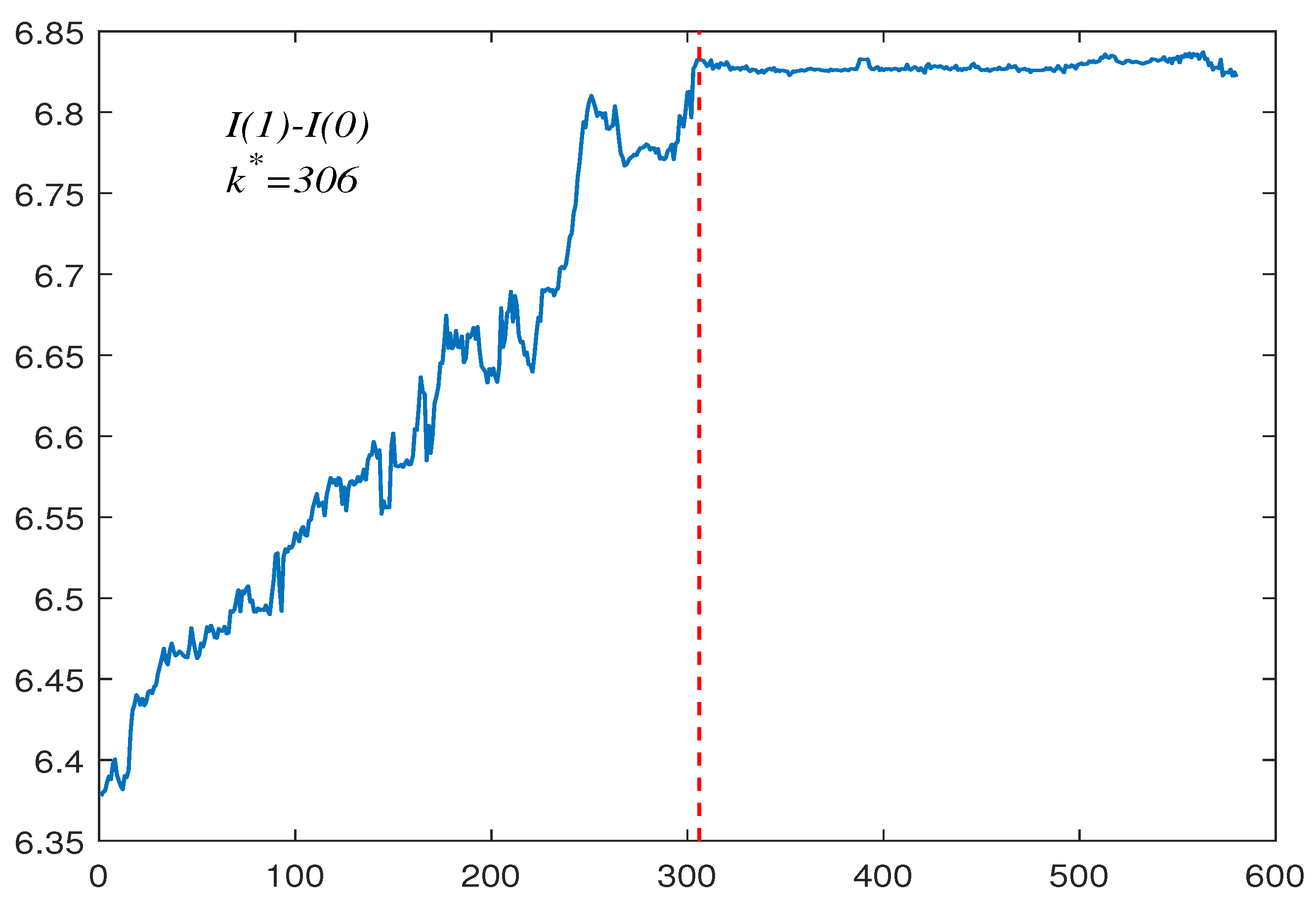
6. Empirical Applications

Especially in many financial time series, the persistence change appears frequently. In this section, we illustrate the proposed test statistic by two examples of time series data, namely data on the US inflation rate and USD/CNY exchange rate which come from multpl.com, and the website of the Federal Reserve Bank of St. Louis, respectively. At the 5% nominal level, we find clear evidence of change from stationary to non-stationary or non-stationary to stationary in these two series.

The first group contains 224 US inflation rate monthly data from September 1958 to April 1977. Figure 1 reports the observations in this set. Chen [33] considered this dataset using a bootstrap test of change in persistence, and concluded that the data contain a change from $I\left(0\right)$ to $I\left(1\right)$. Moreover, they also derived that the estimated change period from $I\left(0\right)$ to $I\left(1\right)$ is May 1965. In this paper, we apply our proposed block bootstrap-based method to verify this conclusion. First, we perform a first-order difference on the data shown in Figure 1 to obtain Figure 2. The differential data were fitted using software provided by John [34] to obtain a tail index of $\widehat{\kappa }=1.8454$ and its corresponding upper- and lower-tail critical values are $8.5203$ and $0.0265$, respectively. As suspected, the existence of a change in persistence is confirmed to be $\Xi =0.0244<0.0264$. This indicates that the data undergo a change from $I\left(0\right)$ to $I\left(1\right)$. The estimated change period from $I\left(0\right)$ to $I\left(1\right)$ is $k^{*}=79$ (May 1965) (see the vertical line in Figure 1). This coincides well with the result obtained by Chen [2]’s.

Figure 1. US inflation rate data $y_t,t=1,\cdots ,224$.

Figure 2. First−order difference in inflation rate data.

The second group contains a 580 USD/CNY exchange rate from 13 May 2009 to 31 August 2011 (see Figure 3). We again fit its first-order difference data in the same way with a tail index of $\widehat{\kappa }=1.0515$. This also reflects that the data contain a lot of outliers. Its corresponding upper- and lower-tail critical values are $5.8298$ and $0.1202$, respectively. The presence of a persistence change is confirmed as $\Xi =5.8441>5.8298$, which also indicates that the data have undergone a change from $I\left(1\right)$ to $I\left(0\right)$. In this example, on the basis of the estimated break fraction $k^{*}=306$ (15 June 2010), it is reasonable to split the whole sample into two regions, where $\left[1306\right]$ is $I\left(1\right)$ and $[307,580]$ is $I\left(0\right)$. To make our conclusion more reliable, we also applied the test proposed by Kim [5], and we found that, on 16 June 2010, the data change from $I\left(1\right)$ to $I\left(0\right)$, which further demonstrate the effectiveness of the method we proposed.

Figure 3. USD/CNY exchange rate data, $y_t,t=1,\cdots ,580$.

Evidently, one may question whether this reject signal was caused by persistence change or those outliers. To test this doubt and make our conclusion more reliable, we also applied our procedure to test the first-order difference data in Figure 2 and Figure 4. The proposed procedure in this paper that used the same parameter choices does not reject the null hypothesis. This result again suggests that the original data undergo a persistence change and the first-order difference data are a stationary sequence. In addition, we divide the two sets of data into two segments according to the estimated break fraction $k^{*}$ and test them separately, before finding that neither of them rejected the null hypothesis. This indicates that there is only one persistence change in both sets of data.

Figure 4. First-order difference in the exchange rate data.

Actually, in the text of the analysis of real-world data, besides for change point models, several ways of analyzing financial time series are possible, such as Cherstvy [35], Yu [36], Kantz [37], who introduced three strategies for the analysis of financial time series based on time-averaged observables, which contained the time-averaged mean-squared displacement as well as the aging and delay time methods for the varying fractions of the financial time series. They found that the observed features of the financial time series dynamics agree well with our analytical results for the time-averaged measurables for geometric Brownian motion, underlying the famed Black–Scholes–Merton model. It was useful for financial data analysis and disclosing new universal features of stock market dynamics.

7. Conclusions

In this paper, we propose a new statistic to test the persistence change with heavy-tailed innovations, and neither the direction of change nor the location of the change can be assumed to be known. We derive the asymptotic distribution of the test statistic under the $H_1$ that is a complicated functional of the $\kappa$-stable process. We also demonstrate that this test is consistent against changes in persistence, either from $I\left(1\right)$ to $I\left(0\right)$ or from $I\left(0\right)$ to $I\left(1\right)$, and prove the consistency of breakpoint estimators. In particular, to determine the critical values for the null distribution of the test statistic containing unknown tail index $\kappa$, we adopt an approach based on the block bootstrap which is a variation on the sampling methodology. The robustness of the block bootstrap method is verified by numerical simulation, and the test obtained displays no tendency of rejecting against constant $I\left(0\right)$ or nearly integrated time series. Empirical applications suggest that our procedures work well in practice. In conclusion, the proposed test statistic based on block bootstrap constitutes a functional tool for detecting changes in persistence with heavy-tailed innovations.

References

- Busetti, F.; Taylor, A.R. Tests of stationarity against a change in persistence. J. Econom. 2004, 123, 33–66. [Google Scholar] [CrossRef]
- Chen, W.; Huang, Z.; Yi, Y. Is there a structural change in the persistence of wti–brent oil price spreads in the post-2010 period? Econ. Model. 2015, 50, 64–71. [Google Scholar] [CrossRef]
- Belaire-Franch, J. A note on the evidence of inflation persistence around the world. Empir. Econ. 2019, 56, 1477–1487. [Google Scholar] [CrossRef]
- Sibbertsen, P.; Willert, J. Testing for a break in persistence under long-range dependencies and mean shifts. Stat. Pap. 2012, 53, 357–370. [Google Scholar] [CrossRef]
- Kim, J.Y. Detection of change in persistence of a linear time series. J. Econom. 2000, 95, 97–116. [Google Scholar] [CrossRef]
- Leybourne, S.; Kim, T.H.; Taylor, A.R. Detecting multiple changes in persistence. Stud. Nonlinear Dyn. Econom. 2007, 11. [Google Scholar] [CrossRef]
- Leybourne, S.; Taylor, R.; Kim, T.H. Cusum of squares-based tests for a change in persistence. J. Time Ser. Anal. 2007, 28, 408–433. [Google Scholar] [CrossRef]
- Cerqueti, R.; Costantini, M.; Gutierrez, L.; Westerlund, J. Panel stationary tests against changes in persistence. Stat. Pap. 2019, 60, 1079–1100. [Google Scholar] [CrossRef]
- Kejriwal, M. A robust sequential procedure for estimating the number of structural changes in persistence. Oxf. Bull. Econ. Stat. 2020, 82, 669–685. [Google Scholar] [CrossRef]
- Hao, J.; Si, Z. Spurious regression between long memory series due to mis-specified structural break. Commun.-Stat.-Simul. Comput. 2018, 47, 692–711. [Google Scholar]
- Hao, J.; Si, Z.; Jinsuo, Z. Modified tests for change point in variance in the possible presence of mean breaks. J. Stat. Comput. Simul. 2018, 88, 2651–2667. [Google Scholar]
- Wingert, S.; Mboya, M.P.; Sibbertsen, P. Distinguishing between breaks in the mean and breaks in persistence under long memory. Econ. Lett. 2020, 193, 1093338. [Google Scholar] [CrossRef]
- Grote, C. Issues in Nonlinear Cointegration, Structural Breaks and Changes in Persistence. Ph.D. Thesis, Leibniz Universität Hannover, Hannover, Germany, 2020. [Google Scholar]
- Mittnik, S.; Rachev, S.; Paolella, M. Stable paretian modeling in finance: Some empirical and theoretical aspects. In A Practical Guide to Heavy Tails; Birkhäuser: Boston, MA, USA, 1998; pp. 79–110. [Google Scholar]
- Han, S.; Tian, Z. Bootstrap testing for changes in persistence with heavy-tailed innovations. Commun. Stat. Theory Methods 2007, 36, 2289–2299. [Google Scholar] [CrossRef]
- Qin, R.; Liu, Y. Block bootstrap testing for changes in persistence with heavy-tailed innovations. Commun. Stat. Theory Methods 2018, 47, 1104–1116. [Google Scholar] [CrossRef]
- Chen, Z.; Tian, Z.; Zhao, C. Monitoring persistence change in infinite variance observations. J. Korean Stat. Soc. 2012, 41, 61–73. [Google Scholar] [CrossRef]
- Yang, Y.; Jin, H. Ratio tests for persistence change with heavy tailed observations. J. Netw. 2014, 9, 1409. [Google Scholar] [CrossRef]
- Hao, J.; Si, Z.; Jinsuo, Z. Spurious regression due to the neglected of non-stationary volatility. Comput. Stat. 2017, 32, 1065–1081. [Google Scholar]
- Hao, J.; Jinsuo, Z.; Si, Z. The spurious regression of AR(p) infinite variance series in presence of structural break. Comput. Stat. Data Anal. 2013, 67, 25–40. [Google Scholar]
- Wang, D. Monitoring persistence change in heavy-tailed observations. Symmetry 2021, 13, 936. [Google Scholar] [CrossRef]
- Chan, N.H.; Zhang, R.M. Inference for nearly nonstationary processes under strong dependence with infinite variance. Stat. Sin. 2009, 19, 925–947. [Google Scholar]
- Cheng, Y.; Hui, Y.; McAleer, M.; Wong, W.K. Spurious relationships for nearly non-stationary series. J. Risk Financ. Manag. 2021, 14, 366. [Google Scholar] [CrossRef]
- Paparoditis, E.; Politis, D.N. Residual-based block bootstrap for unit root testing. Econometrica 2003, 71, 813–855. [Google Scholar] [CrossRef]
- Chan, N.H.; Wei, C.Z. Asymptotic inference for nearly nonstationary AR(1) processes. Ann. Stat. 1987, 15, 1050–1063. [Google Scholar] [CrossRef]
- Leybourne, S.J.; Kim, T.H.; Robert Taylor, A. Regression-based tests for a change in persistence. Oxf. Bull. Econ. Stat. 2006, 68, 595–621. [Google Scholar] [CrossRef]
- Phillips, P.C.; Solo, V. Asymptotics for linear processes. Ann. Stat. 1992, 20, 971–1001. [Google Scholar] [CrossRef]
- Ibragimov, I.A. Some limit theorems for stationary processes. Theory Probab. Appl. 1962, 7, 349–382. [Google Scholar] [CrossRef]
- Resnick, S.I. Point processes, regular variation and weak convergence. Adv. Appl. Probab. 1986, 18, 66–138. [Google Scholar] [CrossRef]
- Chan, N.H. Inference for near-integrated time series with infinite variance. J. Am. Assoc. 1990, 85, 1069–1074. [Google Scholar] [CrossRef]
- Mandelbrot, B. The variation of some other speculative prices. J. Bus. 1967, 40, 393–413. [Google Scholar] [CrossRef]
- Arcones, M.A.; Giné, E. The bootstrap of the mean with arbitrary bootstrap sample size. Ann. IHP Probab. Stat. 1989, 25, 457–481. [Google Scholar]
- Chen, Z.; Jin, Z.; Tian, Z.; Qi, P. Bootstrap testing multiple changes in persistence for a heavy-tailed sequence. Comput. Stat. Data Anal. 2012, 56, 2303–2316. [Google Scholar] [CrossRef]
- John, P.N. Numerical calculation of stable densities and distribution functions. Commun. Stat. Stoch. Model. 1997, 13, 759–774. [Google Scholar]
- Cherstvy, A.G.; Vinod, D.; Aghion, E.; Chechkin, A.V.; Metzler, R. Time averaging, ageing and delay analysis of financial time series. New J. Phys. 2017, 19, 063045. [Google Scholar] [CrossRef]
- Yu, Z.; Gao, H.; Cong, X.; Wu, N.; Song, H.H. A Survey on Cyber-Physical Systems Security. IEEE Internet Things J. 2023, 10, 21670–21686. [Google Scholar] [CrossRef]
- Kantz, H.; Schreiber, T. Nonlinear Time Series Analysis; Cambridge University Press: Cambridge, UK, 2004. [Google Scholar]
- Knight, K. Limit theory for autoregressive-parameter estimates in an infinite-variance random walk. Can. J. Stat. 1989, 17, 261–278. [Google Scholar] [CrossRef]
- Amemiya, T. Regression analysis when the dependent variable is truncated normal. Econom. Econom. Soc. 1973, 41, 997–1016. [Google Scholar] [CrossRef]
Disclaimer/Publisher’s Note: The statements, opinions and data contained in all publications are solely those of the individual author(s) and contributor(s) and not of MDPI and/or the editor(s). MDPI and/or the editor(s) disclaim responsibility for any injury to people or property resulting from any ideas, methods, instructions or products referred to in the content. |
© 2024 by the authors. Licensee MDPI, Basel, Switzerland. This article is an open access article distributed under the terms and conditions of the Creative Commons Attribution (CC BY) license (https://creativecommons.org/licenses/by/4.0/).