Joint Approach for Vehicle Routing Problems Based on Genetic Algorithm and Graph Convolutional Network

Abstract

The logistics demands of industries represented by e-commerce have experienced explosive growth in recent years. Vehicle path-planning plays a crucial role in optimization systems for logistics and distribution. A path-planning scheme suitable for an actual scenario is the key to reducing costs and improving service efficiency in logistics industries. In complex application scenarios, however, it is difficult for conventional heuristic algorithms to ensure the quality of solutions for vehicle routing problems. This study proposes a joint approach based on the genetic algorithm and graph convolutional network for solving the capacitated vehicle routing problem with multiple distribution centers. First, we use the heuristic method to modularize the complex environment and encode each module based on the constraint conditions. Next, the graph convolutional network is adopted for feature embedding for the graph representation of the vehicle routing problem, and multiple decoders are used to increase the diversity of the solution space. Meanwhile, the REINFORCE algorithm with a baseline is employed to train the model, ensuring quick returns of high-quality solutions. Moreover, the fitness function is calculated based on the solution to each module, and the genetic algorithm is employed to seek the optimal solution on a global scale. Finally, the effectiveness of the proposed framework is validated through experiments at different scales and comparisons with other algorithms. The experimental results show that, compared to the single decoder GCN-based solving method, the method proposed in this paper improves the solving success rate to 100% across 15 generated instances. The average path length obtained is only 11% of the optimal solution produced by the GCN-based multi-decoder method.

1. Introduction

As a core issue in logistics and distribution, the vehicle routing problem (VRP) is a typical NP-hard problem in combinatorial optimization [1]. It involves effectively allocating a group of vehicles to access multiple customer points and minimizing the total travel distance or cost while satisfying constraints [2]. With the in-depth study of VRPs, many new VRP variants have been derived in different application scenarios, such as the capacitated vehicle routing problem (CVRP) [3], the vehicle routing problem with time windows (VRPTW) [4], and the split delivery vehicle routing problem (SDVRP) [5].

Although the VRP and its variants have attracted a lot of attention from scholars, the many excellent solutions witnessed are mostly applied in scenarios where the node size is small and the distribution center is unique. In recent years, with the large-scale development of China’s e-commerce, the more common VRP variant has involved multiple distribution centers and large-scale network nodes. Compared to the theoretical research that only considers the optimality of the objective function, the VRP in real-world scenarios demands a reliable path-planning scheme within a limited solution time. The time required for conventional algorithms to solve the VRP increases exponentially with the size of the problem, and if the size or known information changes, the parameters must be adjusted again. Therefore, the efficiency and flexibility of the solution need to be improved. In methods based on learning, such as deep learning and reinforcement learning, hidden features are extracted from massive data or empirical trajectories [6], and the functional relationship between input and output is established through repeated training. For data with the same or similar features, learning-based algorithms can rapidly output results, avoiding repeated searches in the solution space and enabling quick solutions to large-scale VRPs in reality. However, using deep reinforcement learning to solve large-scale VRPs faces problems such as inaccurate network feature extraction and memory overflow. Therefore, this paper proposes a joint approach based on the genetic algorithm (GA) and a graph convolutional network (GCN), aiming to solve the large-scale VRP with multiple distribution centers in an end-to-end manner. The main innovations and contributions of the study are as follows.

(1)

A new algorithm for solving large-scale VRPs with multiple distribution centers is proposed by integrating the ideas of GA and GCN. The proposed method uses GCN to directly extract features from the topology graph without the need for data preprocessing. Additionally, the solution process of the VRP does not rely on any manually designed heuristic operation methods. For VRP instances with the same or similar features, results can be obtained directly, leading to high-quality solutions in a short time.

(2)

In larger-scale instances, this method uses a genetic algorithm to divide complex problems, reducing the search space and effectively avoiding the issue of dimensional explosion.

(3)

In cases where the problem’s constraints change, a solution that satisfies the constraints can be obtained by simply modifying the encoding method of the genetic algorithm, fully leveraging the existing learning experience without the need for retraining.

The rest of this paper is arranged as follows. Section 2 presents the related work. Section 3 introduces the basic process of using the GCN to solve the VRP. Section 4 elaborates on the joint approach based on GA and GCN. Section 5 provides the experimental results. Finally, Section 6 summarizes this study.

2. Related Work

As shown in Figure 1, the algorithms for solving VRPs can be divided into four categories depending on their properties [7]: exact algorithms [8], heuristic algorithms [9], meta-heuristic algorithms [10], and machine learning algorithms [11].

Figure 1. Classification of algorithms for solving VRPs.

The exact algorithms for solving VRPs mainly include the branch and bound [12], branch and price [13], Lagrangian relaxation algorithm [14], and Benders decomposition algorithm [15]. Due to the excellent solution quality achieved by exact algorithms in solving the fundamental problems of combinatorial optimization, researchers have applied them to the VRP and its various variants. For example, Lysgaard et al. [16] added new branching criteria, node selection criteria, and cutting equations to the conventional branch and bound algorithm, enhancing the efficiency in reducing the solution set. Barnhart et al. [17] discussed the use of exact algorithms such as column generation and branch and bound for solving large-scale VRPs. Fukasawa et al. [18] used the branch and price algorithm to solve the CVRP, experimentally proving that the optimal solution could be achieved at large problem scales. When solving the VRPTW with cut delivery, Luo et al. [19] included constraints on cut delivery and time windows in the branch and price algorithm, finding optimal solutions for small-scale problems. Li et al. [20] used the branch and price method to solve VRPs with complex constraints and verified the optimality of their solution via comparison with commercial solvers. Considering the time windows and packing constraints, Ropke et al. [21] employed the branch and bound algorithm and priced the two constraints separately. Exact algorithms outperform other algorithms in terms of solution quality. However, since the essence of exact algorithms is to make cuts in the solution space, when the problem instance size increases, the solution space is prone to exponential explosion, resulting in a low solving efficiency and difficulties in obtaining the optimal solution in a short time.

The core of heuristic algorithms for solving VRPs is to iteratively constrain the root problem of customer nodes that have not yet been served according to the specific constraints and manually set criteria, thereby obtaining an acceptable solution. Clarke et al. [22] designed the Clarke–Wright saving algorithm, which constructed a solution to the VRP by following the principle of adding nodes with fewer saved values first. Altinel et al. [23] included the impact of vehicle capacity limitations on customer node demands based on the Clarke–Wright saving algorithm, obtaining a better solution compared to conventional saving algorithms. Li et al. [24] proposed a two-stage heuristic algorithm based on the algorithms of saving and local search. Comparative experiments were conducted for randomly generated small-scale instances and classical examples to verify the quality and effectiveness of the algorithm’s solution. Bauer et al. [25] simplified the cable layout problem of finding the lowest cost for a VRP and designed a two-stage heuristic algorithm based on conventional saving algorithms. Experimental results showed that the algorithm’s solving efficiency was significantly improved. Heuristic algorithms involve a summary of problem patterns based on human experience, with relatively simple logic. However, these algorithms have poor generalization ability, are prone to local optima, and often suffer from a significant gap between the obtained and optimal solutions for large-scale problems.

To overcome the limitations of heuristic algorithms, researchers have designed a series of meta-heuristic algorithms, whose most distinctive feature from heuristic algorithms is that they can, according to their strategy, accept inferior solutions under certain conditions in the solving process. This configuration expands the search space and enables the algorithms to escape from local optima. Glover [26] first proposed and systematically explained the concept of tabu search for solving nonlinear coverage problems, laying the theoretical foundation for tabu search algorithms [27,28]. According to the problem requirements, Zachariadis et al. [29] added the principle of the local search algorithm to tabu search and successfully solved the VRP under two-dimensional spatial packing constraints. However, a major drawback of tabu search is its excessive reliance on the quality of the initial solution, so tabu search algorithms are often combined with heuristic algorithms. Simulated annealing (SA) [30] is a stochastic optimization algorithm based on the Monte Carlo iterative solution strategy. Kirkpatrick et al. [31] successfully introduced SA into the field of combinatorial optimization. Li [32] incorporated the greedy algorithm with SA and constructed an initial solution for SA, solving large-scale VRPs of heterogeneous vehicles. Mu [33] combined heuristic algorithms with SA to construct a two-stage SA algorithm for solving VRPTWs. In addition, GAs [34], ant colony algorithms [35], and particle swarm optimization algorithms [36] have also been applied to various VRPs due to their efficient solution capabilities. Compared to conventional heuristic algorithms that perform the global search without emphasis, meta-heuristic algorithms can focus on unsearched or potential areas through certain search rules and memory lists, thus having higher efficiency [37].

Despite a high solution efficiency, meta-heuristic algorithms, like exact and heuristic algorithms, still require sufficient, professional domain knowledge to model problems or design effective search rules. When the problem constraints change, the algorithm often needs to make significant changes. With the rise of artificial intelligence, increasingly more scholars have considered using machine learning-based methods to enable agents to acquire the ability to autonomously solve problems [38]. Machine learning-based methods can be divided into three types according to the model training characteristics: supervised learning [39], unsupervised learning [40], and reinforcement learning [41]. However, regardless of the learning paradigm, when solving combinatorial optimization problems, artificial neural networks (ANNs) [42] are required to extract features or fit functions. However, conventional neural networks rely on the assumption that data samples are independent of each other and require fixed-length inputs and outputs, which are difficult to meet in VRPs [43]. Therefore, more researchers have resorted to the pointer network (PN) [44] and graph neural network (GNN) [45] to solve VRPs.

Bello et al. [46] employed reinforcement learning to train the PN model, which achieved better solutions in problems with larger node sizes. On this basis, Nazari et al. [47] adjusted the input layer and replaced the long short-term memory (LSTM) with convolutional layers, which reduced the computational cost. Scarselli et al. [48] leveraged the GNN to learn the features of each node for node prediction. Ma et al. [49] combined the PN with GNN to propose the graph pointer network (GPN), which extracted node features using the GNN and constructed solutions using the PN, thereby improving the algorithm’s generalization performance. Khalil et al. [50] first proposed using the GNN to solve problems. Manchanda et al. [51] further introduced the GCN to solve problems. Hu et al. [52] proposed a bidirectional graph neural network (BGNN) that generated the next access node sequentially through imitation learning, which could be combined with heuristic search to further improve performance. Enrique et al. [53] designed a neural network based on an attention mechanism as a meta-learner to solve the algorithm selection problem, and the experimental results proved that the algorithm selected by the model achieved better results than the benchmark algorithm in different VRPTW instances. Ivan et al. [54] designed a regression machine learning model that captures the input features of the VRP problem while incorporating the output data obtained from the genetic algorithm to directly predict the outcome of the problem without iterative solving. Fitzpatrick et al. [55] proposed a hybrid algorithm based on machine learning and integer linear programming that addresses the problem of poor performance of end-to-end machine learning approaches in large CRVP instances and validates the effectiveness of the algorithm in large-scale instances with hundreds to thousands of nodes. Lagos et al. [56] used Markov models to generate a large number of sequences of low-level heuristic algorithms, employed a machine learning approach to learn the key parameters of the algorithms, and experimentally demonstrated that the proposed hybrid approach based on machine learning and heuristic algorithms achieves competitive results in the VRPTW instance.

It can be seen that machine learning-based methods and their hybrid algorithms achieve better results in larger VRP instances because they have some autonomous problem solving ability and do not need to repeat iterations to solve similar problems; however, these algorithms often require a lot of time to pretrain the model and need to retrain the model when the algorithm constraints are changed, which results in poorer generalizability. The joint solution framework proposed in this paper makes full use of the advantages of machine learning methods without repeated iterations and the flexibility of meta-heuristic algorithms in solving problems with different constraints, and it only requires small-scale changes in the face of changes to the problem scale and constraints, without retraining.

3. Multi-Decoder Architecture for Solving VRPs

This study constructs an end-to-end solution, the primary framework of which is shown in Figure 2. First, the location maps of the distribution centers and service nodes are taken as raw inputs. Then, the GCN is used as an encoder, which is combined with the classical graph search algorithm to calculate the high-dimensional spatial representations or embedded features. Finally, a decoder is employed to predict the probability of node outputs and search for the solution to the problem.

Figure 2. Primary framework of the end-to-end algorithm.

Since the GCN can directly extract features from the node graphs, we need to model VRP instances using theories of graph optimization.

We can consider the VRP instance shown in Figure 3 as a graph $G=(V,E)$, where V is a set of vertices represented by Equation (1):

$$V=\{0,1,2,\cdots ,n\},$$

(1)

where $i=0$ represents the distribution center, and $i=1,2,\cdots ,n$ are the service nodes. The edge set E is represented by Equation (2):

$$E=\left\{e_{ij}\right\},i,j\in V.$$

(2)

Figure 3. VRP instance.

The elements $e_{ij}$ in the set are within the range of $\{0,1\}$. When $e_{ij}=1$, it means that nodes i and j are connected; $e_{ij}=0$ means that i and j are disconnected. All nodes have a coordinate feature $x_i^c$, and the service nodes in the CVRP also have an additional demand feature $x_i^d$.

For VRP, the objective function is to minimize the total travel distance or cost, as shown in Equation (3):

$$min\sum _{k=1}^m\sum _{i=1}^n\sum _{j=1}^n{c}_{ij}{e}_{ij}^k,$$

(3)

where m is the number of vehicles, and $c_{ij}$ is the distance or loss from node i to node j. If vehicle k is accessed from node i to node j, then $e_{ij}^k=1$; otherwise, $e_{ij}^k=0$. The VRP usually has the following constraints [57].

(1)

Node constraint: As shown in Equation (4), each node must be visited and visited only once.

$$\sum _{k=1}^m\sum _{j=1}^n{e}_{ij}^k=1,\forall i\in V$$

(4)

(2)

Path constraints: As shown in Equation (5), each vehicle’s path must start at node 0 and end at node 0.

$$\begin{array}{cc}\hfill & \sum _{j=1}^n{e}_{0j}^k=1,k=1,\cdots ,m\hfill \\ \hfill & \sum _{j=1}^n{e}_{i0}^k=1,k=1,\cdots ,m\hfill \end{array}$$

(5)

(3)

Flow conservation constraints: As shown in Equation (6), for any node (including node 0), after the flow enters the node, an equal amount of flow must exit the node.

$$\begin{array}{c}\hfill \sum _{i\in V}{e}_{ip}^k=\sum _{j\in V}{e}_{pj}^k,\forall p\in V,k=1,\cdots ,m\end{array}$$

(6)

(4)

Binary constraint: $e_{ij}^k\in \{0,1\},\forall i,j\in V,k=0,\cdots ,m$.

(5)

For CVRP, there is a vehicle capacity constraint, as shown in Equation (7):

$$\sum _{j=1}^n{d}_j{e}_{ij}^k\le Q^k,\forall i\in V,k=1,\cdots ,m,$$

(7)

where $d_j$ represents the demand of node j, and $Q^k$ represents the capacity of vehicle k.

3.1. GCN

The process by which GCN learns on graph structure data can be roughly summarized as follows.

(1)

Feature Aggregation: For each node, the feature update is given by Equation (8):

$$H^{(l+1)}=\sigma \left(D^{-{\displaystyle \frac{1}{2}}}A{D}^{-{\displaystyle \frac{1}{2}}}{H}^{\left(l\right)}{W}^{\left(l\right)}\right),$$

(8)

where $H^{\left(l\right)}$ is the node feature matrix at layer l, A is the adjacency matrix of the graph, D is the degree matrix, $W^{\left(l\right)}$ is the learnable weight matrix at layer l, and $\sigma$ is the activation function (such as ReLU).

(2)

Input Feature Matrix: In the first layer of GCN, the input feature matrix is usually:

$$H^{\left(0\right)}=X,$$

(9)

where X is the feature matrix of the input nodes.

(3)

Multi-Layer Stacking: By stacking multiple layers, the final output feature matrix is shown in Equation (10):

$$H^{\left(L\right)}=\sigma \left(D^{-{\displaystyle \frac{1}{2}}}A{D}^{-{\displaystyle \frac{1}{2}}}{H}^{(L-1)}{W}^{(L-1)}\right),$$

(10)

where L denotes the total number of layers.

(4)

Classification Output: Finally, the classification result output through the fully connected layer is:

$$Y=\mathrm{softmax}\left(H^{\left(L\right)}{W}^{\left(L\right)}\right).$$

(11)

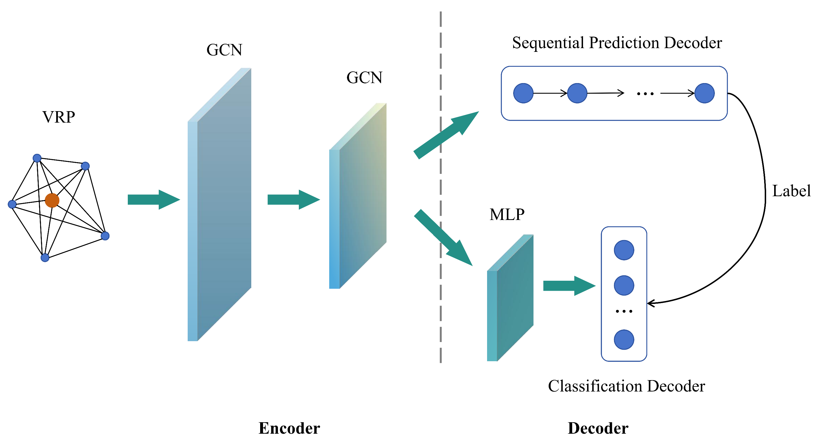
3.2. A New Solution Framework

In small-scale scenarios, using the framework above can yield a high-quality solution. However, for large-scale problems, the algorithm using only a single decoder is easily trapped in local optima. Therefore, a multi-decoder strategy is considered to enable the algorithm to quickly return high-quality solutions. The new solution framework is shown in Figure 4.

Figure 4. Multi-decoder solution framework.

Unlike the traditional single encoder–decoder architecture [48,49,50,51], the new framework adopts two separate decoders on top of the framework shown in Figure 4. One is a sequential prediction decoder based on a recurrent neural network (RNN) [58] or LSTM [59] with node embedding as input, which outputs a predicted sequence as a VRP solution. The other is a classification decoder based on the multi-layer perceptron (MLP) [60], which also takes node embedding as input and a probability matrix as output. The value of the matrix elements represents the probability of the corresponding edges appearing in the solution. One major advantage of using two decoders is that we use reinforcement learning algorithms to train the sequence prediction decoder, and the output results serve as labels for the classification decoder. During the training process, optimizing the loss function of the sequence prediction decoder can indirectly enhance the performance of the classification decoder. Conversely, when the performance of the classification decoder improves, the sequence prediction decoder can better adjust its prediction strategy, leading to more accurate sequence generation. We have already added the above discussion to the article. The specific solution process is as follows.

Input: For each node i in the given graph $G=(V,E)$, initialize it as a feature vector $x_i$ as shown in Equation (12) using the ReLU activation function:

$$x_i=\left\{\begin{array}{cc}\mathrm{ReLU}(W_1{x}_0^c+b_1)& i=0\\ \mathrm{ReLU}\left([W_2{x}_i^c+b_2;W_3{x}_i^d+b_3]\right)& i\ne 0\end{array}\right.,$$

(12)

where [;] is the concat operation, W and b are parameters, and the edge feature $y_{ij}$ is related to the adjacency and distance ($m_{ij}$) of nodes $(i,j)$. We define the following adjacency matrix $A\in R^{(n+1)\times (n+1)}$:

$$a_{ij}\left\{\begin{array}{ccc}1& & \mathrm{if}i\mathrm{and}j\mathrm{are}k-\mathrm{nearest}\mathrm{neighbors}\\ -1& & \mathrm{if}i=j\\ 0& & others\end{array}\right..$$

(13)

It should be noted that, if nodes i and j are k-nearest neighbors, we consider them adjacent. The feature $y_{ij}$ can then be represented as follows:

$$y_{ij}=\mathrm{ReLU}\left([W_4{m}_{ij}+b_4;W_5{a}_{ij}+b_5]\right).$$

(14)

Encode: After determining the node and edge features, we use the decoder for embedding, essentially mapping the two features linearly as shown in Equation (15):

$$\begin{array}{cc}\hfill h_i^0& =W_{E1}{x}_i+b_{E1},\hfill \\ \hfill h_{e_{ij}}^0& =W_{E2}{y}_{ij}+b_{E2}.\hfill \end{array}$$

(15)

Afterward, the mapping function will pass through an L-layer graph convolutional layer, and for each layer $l(l=1,2,\cdots ,L)$, there are two sub-layers: aggregation and combination. The node embedding after l layers is defined as follows:

$$\begin{array}{cc}\hfill h_{N\left(i\right)}^l& =\sigma \left(W^{l}AGG\left(\{h_{i^{\prime }}^{l-1},\forall i^{\prime }\in N\left(i\right)\}\right)\right),\hfill \\ \hfill h_i^l& =COMBINE(h_i^{l-1},h_{N\left(i\right)}^l),\hfill \end{array}$$

(16)

where $h_{N\left(i\right)}^l$ denotes the aggregation feature representing all adjacent nodes $N\left(i\right)$ of node i; AGG is an aggregation function that can be customized according to the specific problem; $\sigma$ is a nonlinear activation function; and COMBINE is a function that embeds a node and its adjacent nodes.

In the aggregation sub-layer, for node $v_i\in V$, the node aggregation embedding can be shown by Equation (17):

$$h_{N\left(i\right)}^l=\sigma \left(W_I^{l}AG{G}_I^l\left(ATTN(h_i^{l-1},\{h_{v^{\prime }}^{l-1},\forall v^{\prime }\in N\left(i\right)\})\right)\right),$$

(17)

where $W_I^l$ is a trainable parameter, and the main role of the ATTN function is to map the feature vector $h_{key}$ and the set of candidate feature vectors $H_{val}$ to a weighted sum of the feature vectors. The ATTN function is represented as follows:

$$f:h_{key}\times H_{val}\to h_{val}.$$

(18)

As for the edge $e_{ij}\in E$, the two nodes connected by the edge need to be considered, so the aggregation embedding of the edge $h_{N\left(e_{ij}\right)}^l$ is defined as shown in Equation (19):

$$\begin{array}{cc}\hfill h_{N\left(e_{ij}\right)}^l& =\sigma \left(W_E^{l}AG{G}_E^l(h_{e_{ij}}^{l-1},h_i^{l-1},h_j^{l-1})\right),\hfill \\ \hfill AG{G}_E^l(h_{e_{ij}}^{l-1},h_i^{l-1},h_j^{l-1})& =W_{e1}^l{h}_{e_{ij}}^l+W_{e2}^l{h}_i^l+W_{e3}^l{h}_j^l.\hfill \end{array}$$

(19)

The combination sub-layer combines $h_{N\left(i\right)}^l$ with $h_{N\left(e_{ij}\right)}^l$ according to the following equation:

$$\begin{array}{cc}\hfill h_i^l& =[V_I^l{h}_i^{l-1};h_{N\left(i\right)}^l],\hfill \\ \hfill h_{e_{ij}}^l& =[V_E^l{h}_{e_{ij}}^{l-1};h_{N\left(e_{ij}\right)}^l],\hfill \end{array}$$

(20)

where $V_I^l$ and $V_E^l$ are the weight matrices to be updated.

Decode: In the sequential prediction decoder, for any input, generate a policy sequence of length T. We hope that the policy sequence $\pi$ generated based on policy $p\left(\pi \right|S;\theta )$ can minimize the objective function. Here, $p\left(\pi \right|S;\theta )$ can be expressed in the form of a joint probability as shown in Equation (21):

$$\begin{array}{cc}\hfill p\left(\pi \right|S;\theta )& =\prod _{t=0}^{T}p\left({\pi }_{t+1}\right|S,{\pi }_t;\theta )\hfill \\ \hfill & =\prod _{t=0}^{T}p\left({\pi }_{t+1}\right|(S,{\theta }_e),{\pi }_t;{\theta }_d),\hfill \end{array}$$

(21)

where $f(S,{\theta }_e)$ is the encoder and ${\theta }_d$ the trainable parameter. Here, a gated recurrent unit (GRU) [61] and a hidden vector $z_t$ are introduced to calculate the last term of Equation (21), as shown in Equation (22):

$$p\left({\pi }_t\right|(S,{\theta }_e),{\pi }_{t-1};{\theta }_d)=p\left({\pi }_{t+1}\right|(S,{\theta }_e),z_t;{\theta }_d).$$

(22)

When decoding, the decoder generates node ${\pi }_t$ based on the node embedding generated by the GCN and the hidden vector $z_t$ of the GRU and finally obtains the policy sequence $\pi$ through iterations. For the specific implementation, we can use the pointer network to calculate the attention score of each node according to the encoding results, obtain the probability distribution after softmax, and finally calculate the output results according to the obtained probability. In the decoding process, at time step t, the context weight $u_{ti}$ of node i is calculated as follows:

$$u_{ti}=\left\{\begin{array}{cc}-\infty & \forall j\in N_{mt}\\ h_a^{T}tanh\left(W^G[v_i;z_t]\right)& otherwise\end{array}\right.,$$

(23)

where $N_{mt}$ is the set of nodes at the current time step, which do not satisfy the constraints, and $h_a^T$ and $W^G$ are the parameters. At this point, Equation (22) can be expressed in the following form:

$$p\left({\pi }_{t+1}\right|(S,{\theta }_e),z_t;{\theta }_d)=\mathrm{softmax}\left(u_{ti}\right).$$

(24)

In a classification decoder, the resulting policy $\pi$ of the sequential prediction decoder can be transformed into a unique path sequence, where edges that appear in the path sequence are denoted as 1 and those that do not are denoted as 0. This leads to a 0–1 matrix $P_E^{VR{P}^{*}}=\left\{p_{e_{ij}}^{VR{P}^{*}}\right\}$ that serves as the label for the classification decoder. By passing the output $h_{e_{ij}}^L$ of the last GCN layer through an MLP, a softmax distribution can be obtained, which can be regarded as the occurrence probability of edge $e_{ij}$, as shown in Equation (25):

$$p_{e_{ij}}^{VRP}=\mathrm{softmax}\left(MLP\left(h_{e_{ij}}^L\right)\right).$$

(25)

So far, we have obtained the probability matrix $p_{e_{ij}}^{VRP}$ through the MLP. This output needs to be as close to $p_{e_{ij}}^{VR{P}^{*}}$ as possible.

3.3. REINFORCE Algorithm

In the process above, we use the REINFORCE algorithm with a baseline to train the policy of the sequential prediction decoder, and its loss function is given in Equation (26):

$$\begin{array}{cc}\hfill L_r({\theta }_e,{\theta }_d)& =\sum _S{E}_{\pi \sim P\left(\pi \right|s;{\theta }_e,{\theta }_d)}(L\left(\pi \right)-b\left(s\right))\hfill \\ \hfill & =\sum _S(L\left(\pi \right)-b\left(s\right))\sum _{i=1}^{T}logp\left({\pi }_i\right|{\pi }_{i-1},S;{\theta }_e,{\theta }_d),\hfill \end{array}$$

(26)

where $L\left(\pi \right)$ denotes the losses caused by policy $\pi$, and the loss from the classification decoder is as follows:

$$L_s({\theta }_e,{\theta }_c)=-\sum _{S,\pi }\mathrm{crossEntropy}(P_E^{VRP},P_E^{VR{P}^{*}}).$$

(27)

In summary, the final loss function $L_{\theta }$ is a linear combination of $L_r({\theta }_e,{\theta }_d)$ and $L_s({\theta }_e,{\theta }_c)$, as shown in Equation (28):

$$L_{\theta }=\alpha L_r({\theta }_e,{\theta }_d)+\beta L_s({\theta }_e,{\theta }_c).$$

(28)

4. A Joint Approach Based on GA and GCN

When the scale of client nodes in VRPs expands, the aforementioned multi-decoder framework built based on the GCN still encounters problems such as memory overflow. Furthermore, in the multi-distribution center VRP shown in Figure 5, the GCN will extract some redundant features, such as the edge features between distribution centers, resulting in a waste of computing power. In reality, the VRP with multiple distribution centers is often constrained by distribution resources, such as a fixed number of distribution vehicles. This means that the resource allocation method can also affect the final solution, and the distribution centers have an impact on each other. Therefore, the multi-center VRP cannot simply be split into several individual VRPs to be solved.

Figure 5. VRP with multiple distribution centers.

To lower the algorithm’s complexity, reduce the solution space, and avoid the extraction of redundant features by the GCN, we introduce the GA into the multi-decoder solution framework above. Via encoding, the constraints of the problem are satisfied, and the search space is narrowed down. Moreover, the heuristic method is employed to split the complex problem into several simple sub-problems, ultimately obtaining high-quality solutions.

For the aforementioned VRP with multiple distribution centers, we use $C=\{c_1,c_2,\cdots ,c_p\}$ and $S=\{s_1,s_2,\cdots ,s_q\}$ to represent the sets of distribution center nodes and customer nodes, respectively. The solution process for this problem is as follows.

(1)

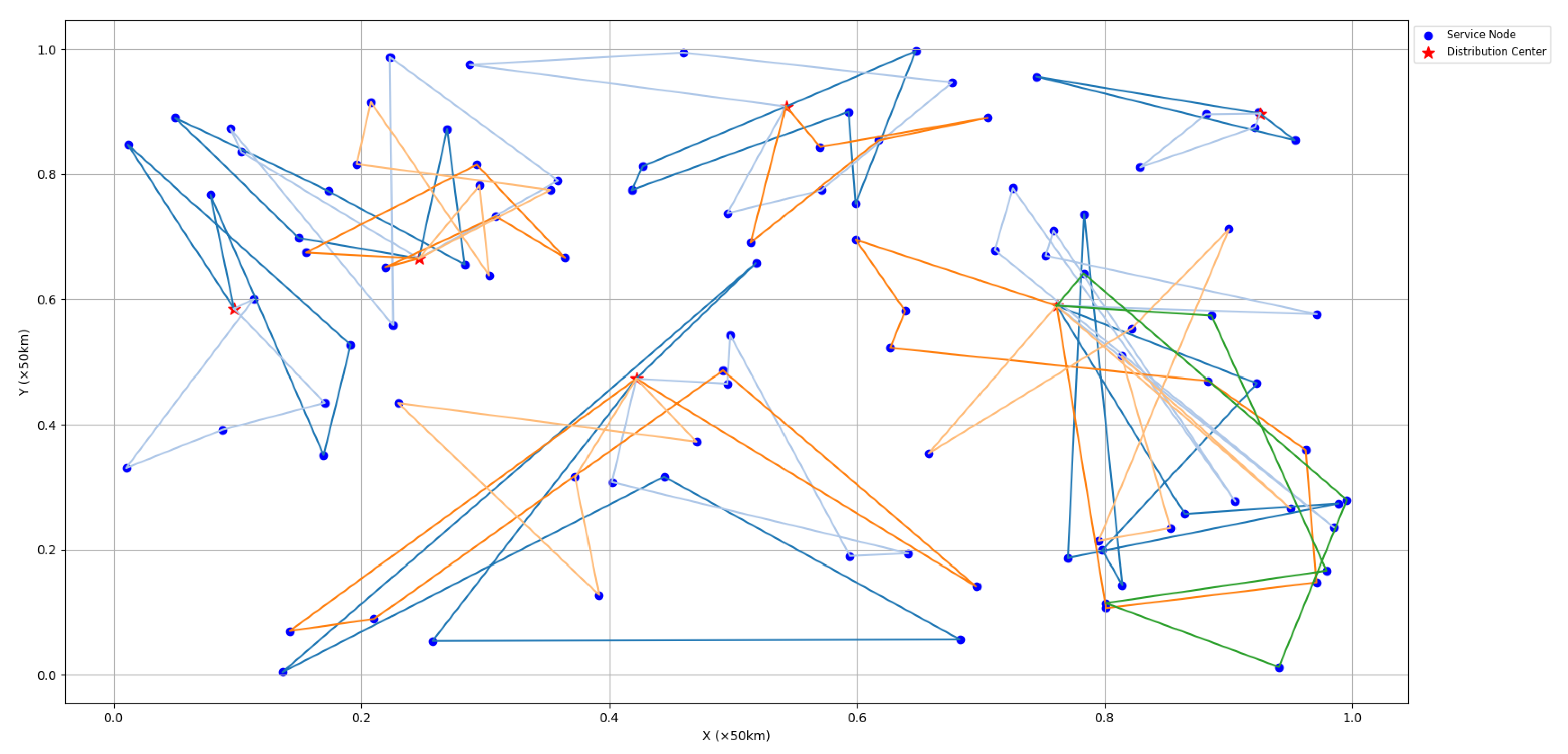
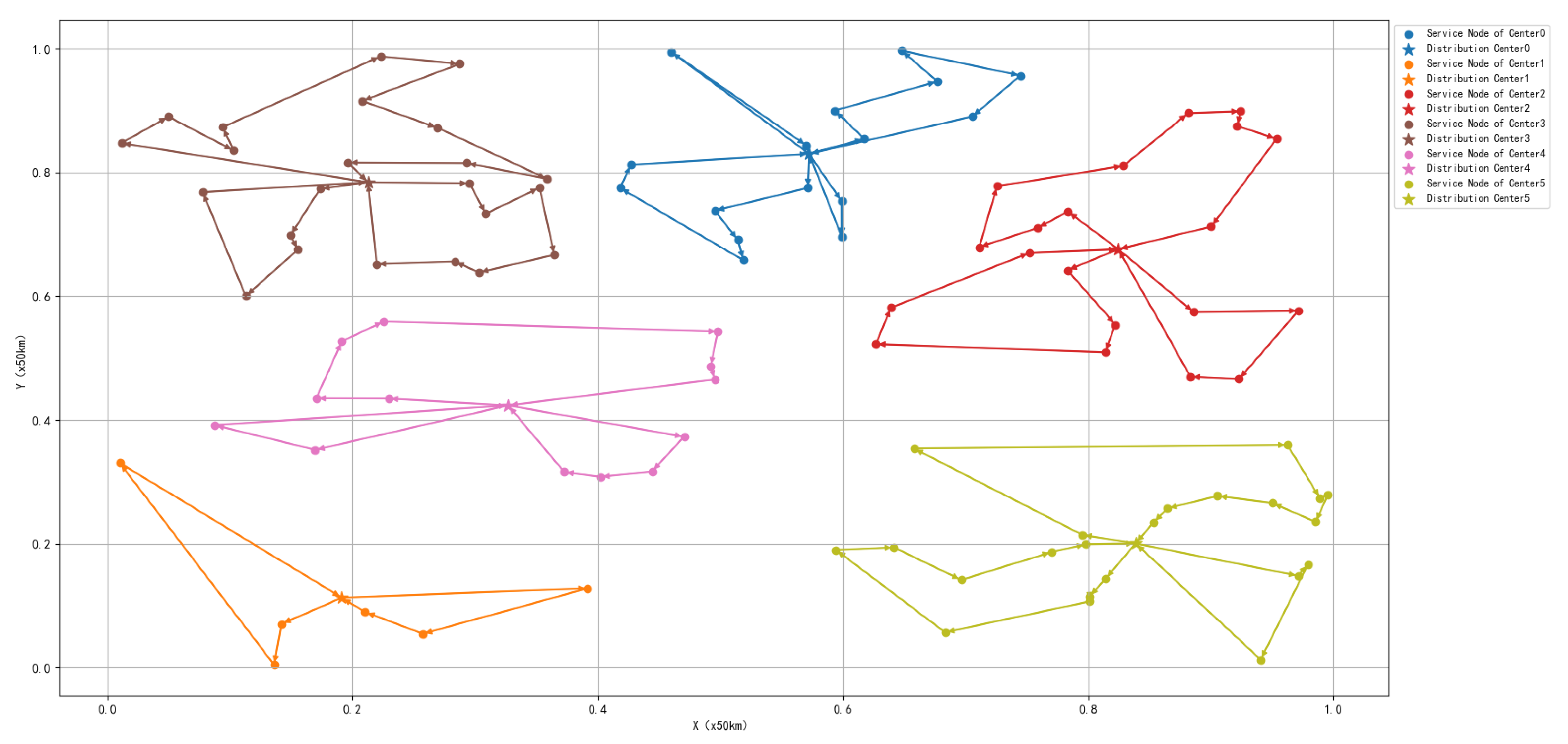
Use the heuristic method to allocate the customer nodes, in which a greedy approach is adopted. For any customer node $s_j$, calculate the Euclidean distance $d(c_i,s_j)$ between it and the distribution center node $c_i,i=1,2,\cdots ,p$ and assign it to the nearest distribution center.

(2)

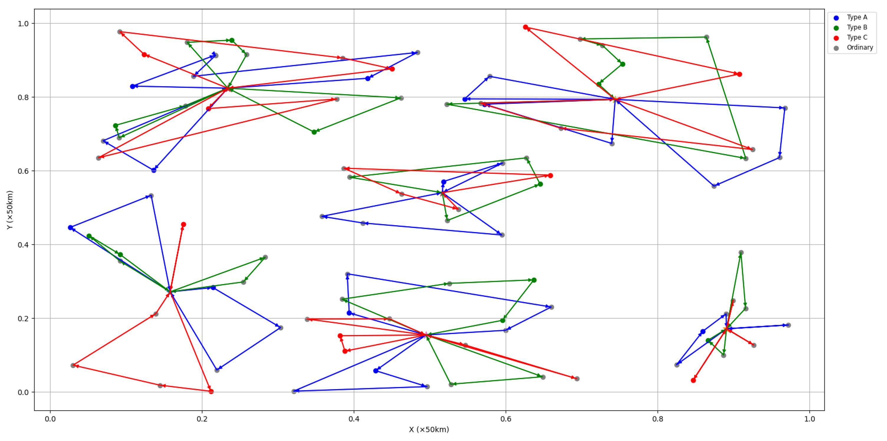
Split the multi-distribution center VRP into p individual VRPs using the method above. Integer encoding is employed to represent the allocation of distribution vehicles, that is, a p-dimensional vector $w=(w_1,\cdots ,w_p)$ is encoded, where each component of the vector represents the number of vehicles allocated to the corresponding distribution center node.

(3)

Use the multi-decoder solution framework to solve the VRP with a fixed number of vehicles and output the optimal policy ${\pi }_i^{*}$.

(4)

Calculate cost $L_i\left({\pi }_i^{*}\right)$ according to Equation (3). The fitness function f can be represented by the following formula:

$$f={\displaystyle \frac{1}{{\displaystyle \sum _{i=1}^p}{L}_i\left({\pi }_i^{*}\right)}}.$$

(29)

(5)

Use the GA to optimize the allocation plan and output the optimum policy under the optimal allocation plan.

The block diagram of the joint approach based on GA and GCN is shown in the below Algorithm 1.

Algorithm 1 Joint Approach Based on GA and GCN

Input:  Distribution center node set C, customer node set S, total number of delivery vehicles M, maximum iteration times N, population size H. Output:  Optimum allocation plan $w_{h^{*}}$, optimal policy ${\pi }^{*}$, and minimum loss $L\left({\pi }^{*}\right)$.   1: Initialize: The GCN network parameters of ${\theta }_e$, ${\theta }_c$, and ${\theta }_d$.   2: Allocate customer node $s_j$ to the nearest distribution center using the greedy algorithm.   3: while $n<N$ do   4:     Encode the vehicle allocation scheme as a p-dimensional vector $w_h=(w_1^h,\cdots ,w_2^h)$, $h=1,2,\cdots ,H$.   5:     for $h=1,2,\cdots ,H$ do   6:         for $i=1,2,\cdots ,p$ do   7:            Use the multi-decoder solution framework to solve the VRP when the vehicle number is fixed at $w_i^h$.   8:            Calculate cost $L_i\left({\pi }_i^{*}\right)$ by Equation (3).   9:            Calculate the individual fitness $f_h$ using Equation (29). 10:            Generate new populations via selection, crossover, and mutation. 11:            $n=n+1$ 12:         end for 13:     end for 14: end while

5. Experimental Results

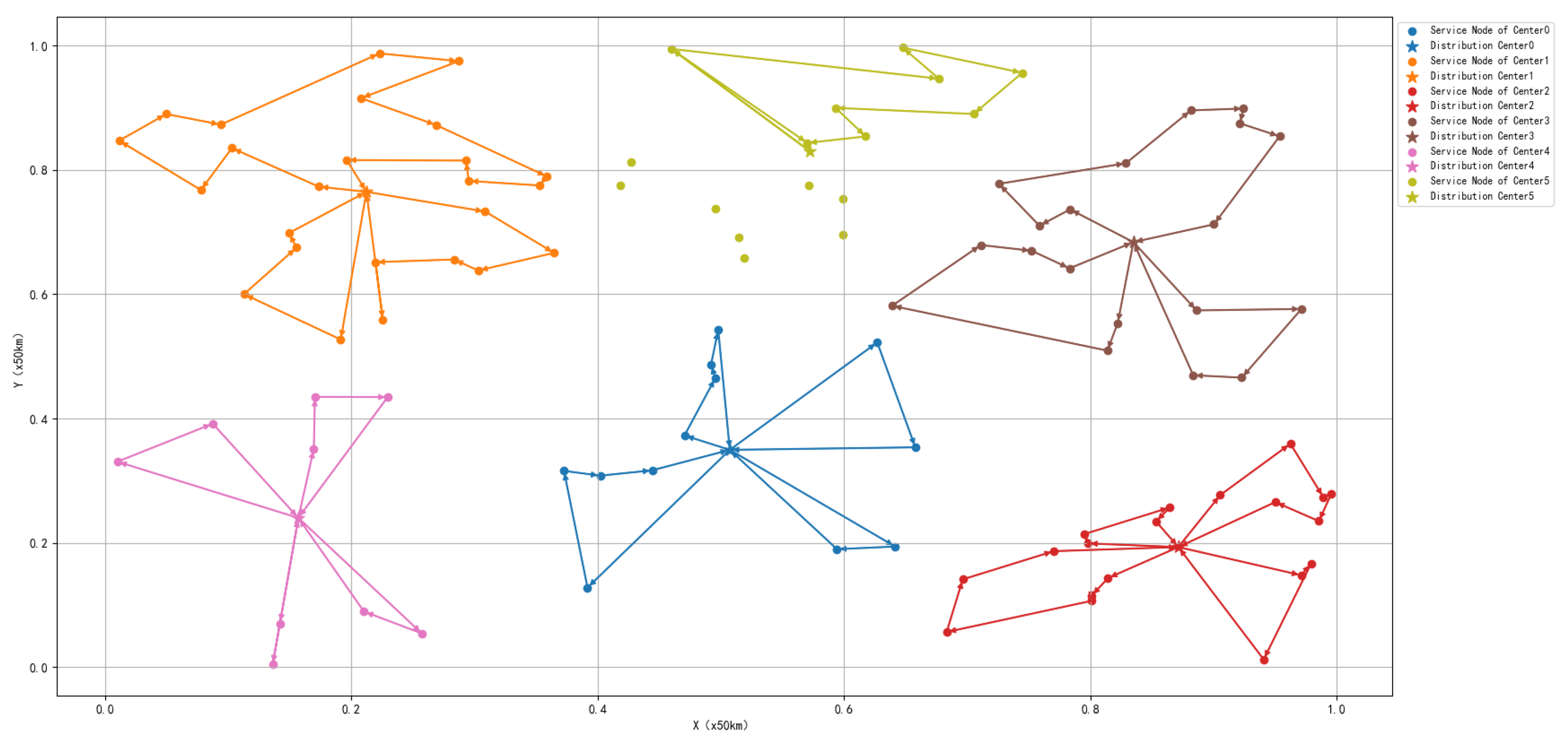
Consider the logistics and distribution problem in a real city. It is now known that there are 100% service nodes in a city, and their locations are distributed as shown in Figure 6. A courier company needs to establish distribution centers in the city. It is known that the company needs to establish a total of 6 distribution centers in the city and, at the same time, 20 teams will be assigned to each center.

Figure 6. Service node locations.

In order to facilitate the subsequent algorithm solution, the coordinates $(x_i,y_i)$ of any node $p_i$ in the graph need to be normalized, and the new coordinates of the node $p_i(x_i^{new},y_i^{new})$ are shown in Equation (30):

$$\begin{array}{cc}\hfill x_i^{new}& ={\displaystyle \frac{x_i}{d_{xmax}}},\hfill \\ \hfill y_i^{new}& ={\displaystyle \frac{y_i}{d_{ymax}}},\hfill \end{array}$$

(30)

where $d_{xmax}$ and $d_{ymax}$ are the maximum value of the absolute value of the difference between the horizontal coordinates of any two nodes $p_m$ and $p_n$, as shown in Equation (31):

$$\begin{array}{cc}\hfill d_{xmax}& =max\left|x_m-x_n\right|,\hfill \\ \hfill d_{ymax}& =max\left|y_m-y_n\right|.\hfill \end{array}$$

(31)

Now the distribution centers need to be located and teams need to be assigned to each center at the same time, and the following constraints need to be followed during the assignment process.

(1)

Minimum constraint: Each center is assigned at least one team.

(2)

Capacity constraint: Each team is required to perform distribution tasks but is responsible for a maximum of 10 service nodes.

The objective is a team allocation and routing plan that obtains the shortest total distance when the teams complete the tasks. Table 1 shows the parameter settings for the single decoder solving method based on GCN, a multi-decoder joint solving method based on GCN, and the joint approach based on GA and GCN. Figure 7, Figure 8 and Figure 9 respectively show the results obtained by the three methods for the problems.

Table 1. Parameter settings for two approaches.

Parameter	Value
greedy learning rate	0.9
learning rate	0.01
max epochs	10,000
discount factor	0.9
batch size	32
normalization parameters	50
population size	300
maximum number of iterations	500
crossover probability	0.5
mutation probability	0.1

Figure 7. Results obtained from the single decoder solving method based on GCN.

Figure 8. Results obtained from the multi-decoder joint solving method based on GCN.

Figure 9. Results obtained from the joint approach.

The experimental results show that the single decoder approach based on GCN failed to generate paths that meet the constraint conditions, as the vehicle forgot some nodes. The multi-decoder approach based on GCN managed to generate paths that meet the constraint conditions, but the paths were relatively complex. In contrast, the hybrid method combining GA and GCN produced better paths that satisfied the constraint conditions. This is because the instance contained a large number of nodes, leading to catastrophic forgetting during the final output sequence in the single decoder approach based on GCN. Although the multi-decoder approach based on GCN avoided the catastrophic forgetting problem by utilizing multiple decoders, in the multi-depot VRP, the network could not effectively eliminate redundant features, resulting in more complex paths. On the other hand, the hybrid approach combining GA and GCN allocated vehicle resources through GA, breaking down the complex problem into simpler sub-problems, successfully avoiding the extraction of redundant features by the GCN network and ultimately generating better paths.

Taking into account the fact that the distribution of service nodes in different cities may be different, a variety of different service node distributions are randomly generated. Table 2 demonstrates the lengths of the team travel paths and the solution times for the three methods with a fixed training time in different multi-distribution center VRPs. Here, “F” signifies that the algorithm failed to plan a path that meets the constraint conditions. It can be observed that, in 15 instances, the success rate of the single decoder method based on GCN is relatively low, while the success rate of the other two algorithms is 100.

Table 2. Results for different multi-distribution center VRPs.

Distribution	Single Decoder Approach		Multi-Decoder Approach		Joint Approach
	$\mathit{d}$ (×50 km)	$\mathit{t}$/s	$\mathit{d}$ (×50 km)	$\mathit{t}$/s	$\mathit{d}$ (×50 km)	$\mathit{t}$/s
1	F	15.29	85.38	16.56	11.52	37.73
2	F	17.66	114.18	19.12	11.68	37.71
3	F	12.48	73.46	19.06	11.85	37.16
4	F	14.28	101.55	16.51	13.14	38.52
5	12.60	16.36	96.11	16.63	12.47	38.26
6	F	13.27	104.11	19.20	12.31	36.96
7	F	14.17	87.49	18.71	11.71	37.55
8	F	15.66	64.50	19.55	11.16	36.61
9	12.08	13.42	130.70	22.81	11.98	37.35
10	F	15.75	90.41	16.39	11.80	36.76
11	F	12.99	105.62	20.43	11.46	36.49
12	F	15.69	90.89	17.46	11.60	37.46
13	F	14.10	175.63	19.58	11.78	37.65
14	F	12.39	100.54	16.33	10.67	37.27
15	F	13.51	74.37	19.50	11.99	37.66

Furthermore, after calculation, the average length of the optimal path obtained by the GCN-based multi-decoder solving method is 99.66 × 50 km, while the result obtained by the method proposed in this paper is 11.80 × 50 km, which is only 11% of the length of the multi-decoder method. Additionally, the variance of the optimal paths solved by the multi-decoder method based on GCN and the joint solving method based on GA and GCN is 721.06 and 0.32, respectively. It can be seen that the joint approach based on GA and GCN achieves better results, and the method is more stable. The reason that the method takes longer is because the genetic algorithm consumes some time in searching for the optimal team allocation scheme.

Considering the reality that some goods have special distribution requirements, such as the need for cold chain transportation, etc., we further add the following constraints on the basis of the above problem: there are three types of special and ordinary goods in the distribution center, A, B, and C, and the ratio of the four types of goods is about 1:1:1:3 corresponding to the three types of distribution teams and whichever type of distribution team can deliver the ordinary goods.

The experimental results show that, within the specified time, the multi-decoder solution framework still cannot obtain feasible solutions, while the joint approach obtains a better solution by merely changing the population encoding scheme. The solution results are given in Figure 10.

Figure 10. VRP solution results for multiple distribution centers under complex constraints.

It can be seen that, when the constraints become more complex, the proposed algorithm can obtain solutions through a simple modification, which is indicative of a strong generalization ability.

To further verify the effectiveness of the algorithm, we generated three VRP instance sets based on the real data of the B2B platform delivery system, whose details are summarized in Table 3. Each instance set includes instances for training and testing.

Table 3. Data for VRP instance sets.

Instance Sets	Number of Service Nodes	Vehicle Capacities	Data Size (Train/Test)
VRP50	50	40	50,000/10,000
VRP200	200	60	25,600/5000
VRP400	400	80	25,600/5000

We consider comparisons with the following state-of-the-art methods, which have been shown to be able to produce near-optimal solutions to the other problem sets:

(1)

OR-Tools: A common heuristic solver proposed by Google [62].

(2)

PRL: A learning model based on deep neural network with an LSTM encoder [47].

(3)

AM: A learning model based on the attention model with coordination embeddings [63]. It is shown to outperform a well-known heuristic for VRP, LKH3 heuristic [64].

(4)

GCN-NPEC: A learning model based on a graph convolutional network with node sequential prediction and edge classification [65].

Considering the different number of problems in different sets, we take the average value of the optimal solution obtained by each method in each set of instances as the evaluation index. In addition, in order to show the experimental results more intuitively, we select the OR-Tools method as the benchmark method and calculate the gap between the current method and the average value obtained by the benchmark method by Equation (32):

$$\begin{array}{c}\hfill {\displaystyle \frac{{\overline{C}}_M-{\overline{C}}_{OR}}{{\overline{C}}_{OR}}}\times 100\end{array},$$

(32)

where ${\overline{C}}_M$ and ${\overline{C}}_{OR}$ are the average values of the optimal solutions obtained by the current method as well as the benchmark method, respectively, and the final experimental results obtained are shown in Table 4.

Table 4. Results of different methods.

Instance Sets	Methods
	OR-Tools	PRL	AM	GCN-NPEC	GCN-GA
VRP50	7.61 (0.00%)	7.79 (2.37%)	7.64 (0.39%)	7.67 (0.79%)	7.71 (1.31%)
VRP200	18.01 (0.00%)	20.12 (11.71%)	18.86 (4.72%)	17.81 (−1.11%)	17.89 (−0.67%)
VRP400	28.13 (0.00%)	30.25 (7.54%)	29.78 (5.87%)	27.05 (−3.84%)	26.89 (−4.41%)

The experimental results show that, in large-scale instances, the results obtained by the GCN-based method are better than the benchmark method. The reason for the similarity between the proposed method and the GCN-NPEC method is that both of them adopt the same network structure, and the GA module in the proposed joint solution framework is not iteratively updated in the VRP instance with only a single distribution center.

6. Conclusions

This paper proposes an end-to-end joint approach based on GA and GCN to solve the large-scale, complexly constrained VRP with multiple distribution centers. Compared to the solution framework that solely uses the GCN, the proposed method adopts a multi-decoder strategy on top of the GCN to increase the spatial diversity of solutions. Additionally, GA is introduced to cope with various constraints, allowing the GCN to focus on solving simple VRPs and improving algorithm efficiency. Ultimately, numerous randomly generated instances prove that the proposed method can quickly obtain higher quality solutions while flexibly responding to changes in constraints, indicating strong generalization abilities.

This study focuses on solving the VRP of multiple distribution centers under a fixed node distribution. However, dynamic factors exist in the actual logistics and distribution process, where the number of customer nodes may increase or decrease, and their locations may change over time. Therefore, we plan to introduce dynamic factors into the problem based on this research, improve the proposed method, and make it adaptable to dynamic VRPs.

References

1. Toth, P.; Vigo, D. The Vehicle Routing Problem; SIAM: Philadelphia, PA, USA, 2002. [Google Scholar]
2. Dantzig, G.B.; Ramser, J.H. The truck dispatching problem. Manag. Sci. 1959, 6, 80–91. [Google Scholar] [CrossRef]
3. Ralphs, T.K.; Kopman, L.; Pulleyblank, W.R.; Trotter, L.E. On the capacitated vehicle routing problem. Math. Program. 2003, 94, 343–359. [Google Scholar] [CrossRef]
4. Tan, K.C.; Lee, L.H.; Zhu, Q.; Ou, K. Heuristic methods for vehicle routing problem with time windows. Artif. Intell. Eng. 2001, 15, 281–295. [Google Scholar] [CrossRef]
5. Archetti, C.; Speranza, M.G. The split delivery vehicle routing problem: A survey. In The Vehicle Routing Problem: Latest Advances and New Challenges; Springer: Boston, MA, USA, 2008; pp. 103–122. [Google Scholar]
6. Song, H.; Triguero, I.; Özcan, E. A review on the self and dual interactions between machine learning and optimisation. Prog. Artif. Intell. 2019, 8, 143–165. [Google Scholar] [CrossRef]
7. Ni, Q.; Tang, Y. A bibliometric visualized analysis and classification of vehicle routing problem research. Sustainability 2023, 15, 7394. [Google Scholar] [CrossRef]
8. Laporte, G.; Nobert, Y. Exact algorithms for the vehicle routing problem. In North-Holland Mathematics Studies; Elsevier: Amsterdam, The Netherlands, 1987; Volume 132, pp. 147–184. [Google Scholar]
9. Kokash, N. An Introduction to Heuristic Algorithms; Department of Informatics and Telecommunications: Trento, Italy, 2005; pp. 1–8. [Google Scholar]
10. Beheshti, Z.; Shamsuddin, S.M.H. A review of population-based meta-heuristic algorithms. Int. J. Adv. Soft Comput. Appl. 2013, 5, 1–35. [Google Scholar]
11. Dietterich, T.G. Machine learning. Annu. Rev. Comput. Sci. 1990, 4, 255–306. [Google Scholar] [CrossRef]
12. Lawler, E.L.; Wood, D.E. Branch-and-bound methods: A survey. Oper. Res. 1966, 14, 699–719. [Google Scholar] [CrossRef]
13. Vanderbeck, F. Branching in branch-and-price: A generic scheme. Math. Program. 2011, 130, 249–294. [Google Scholar] [CrossRef]
14. Fisher, M.L. An applications oriented guide to Lagrangian relaxation. Interfaces 1985, 15, 10–21. [Google Scholar] [CrossRef]
15. Geoffrion, A.M. Generalized benders decomposition. J. Optim. Theory Appl. 1972, 10, 237–260. [Google Scholar] [CrossRef]
16. Lysgaard, J.; Letchford, A.N.; Eglese, R.W. A new branch-and-cut algorithm for the capacitated vehicle routing problem. Math. Program. 2004, 100, 423–445. [Google Scholar] [CrossRef]
17. Barnhart, C.; Johnson, E.L.; Nemhauser, G.L.; Savelsbergh, M.W.; Vance, P.H. Branch-and-price: Column generation for solving huge integer programs. Oper. Res. 1998, 46, 316–329. [Google Scholar] [CrossRef]
18. Fukasawa, R.; Longo, H.; Lysgaard, J.; Aragão, M.P.d.; Reis, M.; Uchoa, E.; Werneck, R.F. Robust branch-and-cut-and-price for the capacitated vehicle routing problem. Math. Program. 2006, 106, 491–511. [Google Scholar] [CrossRef]
19. Luo, Z.; Qin, H.; Zhu, W.; Lim, A. Branch and price and cut for the split-delivery vehicle routing problem with time windows and linear weight-related cost. Transp. Sci. 2017, 51, 668–687. [Google Scholar] [CrossRef]
20. Li, J.; Qin, H.; Baldacci, R.; Zhu, W. Branch-and-price-and-cut for the synchronized vehicle routing problem with split delivery, proportional service time and multiple time windows. Transp. Res. Part E Logist. Transp. Rev. 2020, 140, 101955. [Google Scholar] [CrossRef]
21. Ropke, S.; Cordeau, J.F. Branch and cut and price for the pickup and delivery problem with time windows. Transp. Sci. 2009, 43, 267–286. [Google Scholar] [CrossRef]
22. Clarke, G.; Wright, J.W. Scheduling of vehicles from a central depot to a number of delivery points. Oper. Res. 1964, 12, 568–581. [Google Scholar] [CrossRef]
23. Altınel, İ.K.; Öncan, T. A new enhancement of the Clarke and Wright savings heuristic for the capacitated vehicle routing problem. J. Oper. Res. Soc. 2005, 56, 954–961. [Google Scholar] [CrossRef]
24. Li, H.; Chang, X.; Zhao, W.; Lu, Y. The vehicle flow formulation and savings-based algorithm for the rollon-rolloff vehicle routing problem. Eur. J. Oper. Res. 2017, 257, 859–869. [Google Scholar] [CrossRef]
25. Bauer, J.; Lysgaard, J. The offshore wind farm array cable layout problem: A planar open vehicle routing problem. J. Oper. Res. Soc. 2015, 66, 360–368. [Google Scholar] [CrossRef]
26. Glover, F. Heuristics for integer programming using surrogate constraints. Decis. Sci. 1977, 8, 156–166. [Google Scholar] [CrossRef]
27. Glover, F. Tabu search—Part I. ORSA J. Comput. 1989, 1, 190–206. [Google Scholar] [CrossRef]
28. Glover, F. Tabu search—Part II. ORSA J. Comput. 1990, 2, 4–32. [Google Scholar] [CrossRef]
29. Zachariadis, E.E.; Tarantilis, C.D.; Kiranoudis, C.T. A guided tabu search for the vehicle routing problem with two-dimensional loading constraints. Eur. J. Oper. Res. 2009, 195, 729–743. [Google Scholar] [CrossRef]
30. Metropolis, N.; Rosenbluth, A.W.; Rosenbluth, M.N.; Teller, A.H.; Teller, E. Equation of state calculations by fast computing machines. J. Chem. Phys. 1953, 21, 1087–1092. [Google Scholar] [CrossRef]
31. Kirkpatrick, S.; Gelatt, C.D., Jr.; Vecchi, M.P. Optimization by simulated annealing. Science 1983, 220, 671–680. [Google Scholar] [CrossRef]
32. Li, B.; Yang, X.; Xuan, H. A hybrid simulated annealing heuristic for multistage heterogeneous fleet scheduling with fleet sizing decisions. J. Adv. Transp. 2019, 2019, 5364201. [Google Scholar] [CrossRef]
33. Mu, D.; Wang, C.; Wang, S.; Zhou, S. Solving TDVRP based on parallel-simulated annealing algorithm. Comput. Integr. Manuf. Syst. 2015, 21, 1626–1636. [Google Scholar]
34. Li, X.; Chen, N.; Ma, H.; Nie, F.; Wang, X. A Parallel Genetic Algorithm With Variable Neighborhood Search for the Vehicle Routing Problem in Forest Fire-Fighting. IEEE Trans. Intell. Transp. Syst. 2024, 15, 14359–14375. [Google Scholar] [CrossRef]
35. Stodola, P.; Kutěj, L. Multi-Depot Vehicle Routing Problem with Drones: Mathematical formulation, solution algorithm and experiments. Expert Syst. Appl. 2024, 241, 122483. [Google Scholar] [CrossRef]
36. Wu, Q.; Xia, X.; Song, H.; Zeng, H.; Xu, X.; Zhang, Y.; Yu, F.; Wu, H. A neighborhood comprehensive learning particle swarm optimization for the vehicle routing problem with time windows. Swarm Evol. Comput. 2024, 84, 101425. [Google Scholar] [CrossRef]
37. Desale, S.; Rasool, A.; Andhale, S.; Rane, P. Heuristic and meta-heuristic algorithms and their relevance to the real world: A survey. Int. J. Comput. Eng. Res. Trends 2015, 351, 2349–7084. [Google Scholar]
38. Adamo, T.; Gendreau, M.; Ghiani, G.; Guerriero, E. A review of recent advances in time-dependent vehicle routing. Eur. J. Oper. Res. 2024, 319, 1–15. [Google Scholar] [CrossRef]
39. Hastie, T.; Tibshirani, R.; Friedman, J.; Hastie, T.; Tibshirani, R.; Friedman, J. Overview of supervised learning. In The Elements of Statistical Learning: Data Mining, Inference, and Prediction; Springer: New York, NY, USA, 2009; pp. 9–41. [Google Scholar]
40. Barlow, H.B. Unsupervised learning. Neural Comput. 1989, 1, 295–311. [Google Scholar] [CrossRef]
41. Sutton, R.S.; Barto, A.G. Reinforcement learning: An introduction. Robotica 1999, 17, 229–235. [Google Scholar] [CrossRef]
42. Abiodun, O.I.; Jantan, A.; Omolara, A.E.; Dada, K.V.; Mohamed, N.A.; Arshad, H. State-of-the-art in artificial neural network applications: A survey. Heliyon 2018, 4, e00938. [Google Scholar] [CrossRef]
43. Lipton, Z.C.; Berkowitz, J.; Elkan, C. A critical review of recurrent neural networks for sequence learning. arXiv 2015, arXiv:1506.00019. [Google Scholar]
44. Vinyals, O.; Fortunato, M.; Jaitly, N. Pointer networks. Adv. Neural Inf. Process. Syst. 2015, 28, 2692–2700. [Google Scholar]
45. Wu, Z.; Pan, S.; Chen, F.; Long, G.; Zhang, C.; Philip, S.Y. A comprehensive survey on graph neural networks. IEEE Trans. Neural Netw. Learn. Syst. 2020, 32, 4–24. [Google Scholar] [CrossRef]
46. Bello, I.; Pham, H.; Le, Q.V.; Norouzi, M.; Bengio, S. Neural combinatorial optimization with reinforcement learning. arXiv 2016, arXiv:1611.09940. [Google Scholar]
47. Nazari, M.; Oroojlooy, A.; Snyder, L.; Takác, M. Reinforcement learning for solving the vehicle routing problem. Adv. Neural Inf. Process. Syst. 2018, 31, 9861–9871. [Google Scholar]
48. Scarselli, F.; Gori, M.; Tsoi, A.C.; Hagenbuchner, M.; Monfardini, G. The graph neural network model. IEEE Trans. Neural Netw. 2008, 20, 61–80. [Google Scholar] [CrossRef] [PubMed]
49. Ma, Q.; Ge, S.; He, D.; Thaker, D.; Drori, I. Combinatorial optimization by graph pointer networks and hierarchical reinforcement learning. arXiv 2019, arXiv:1911.04936. [Google Scholar]
50. Khalil, E.; Dai, H.; Zhang, Y.; Dilkina, B.; Song, L. Learning combinatorial optimization algorithms over graphs. Adv. Neural Inf. Process. Syst. 2017, 30, 6351–6361. [Google Scholar]
51. Mittal, A.; Dhawan, A.; Medya, S.; Ranu, S.; Singh, A. Learning heuristics over large graphs via deep reinforcement learning. arXiv 2019, arXiv:1903.03332. [Google Scholar]
52. Hu, Y.; Zhang, Z.; Yao, Y.; Huyan, X.; Zhou, X.; Lee, W.S. A bidirectional graph neural network for traveling salesman problems on arbitrary symmetric graphs. Eng. Appl. Artif. Intell. 2021, 97, 104061. [Google Scholar] [CrossRef]
53. Díaz de León-Hicks, E.; Conant-Pablos, S.E.; Ortiz-Bayliss, J.C.; Terashima-Marín, H. Addressing the algorithm selection problem through an attention-based meta-learner approach. Appl. Sci. 2023, 13, 4601. [Google Scholar] [CrossRef]
54. Singgih, I.K.; Singgih, M.L. Regression Machine Learning Models for the Short-Time Prediction of Genetic Algorithm Results in a Vehicle Routing Problem. World Electr. Veh. J. 2024, 15, 308. [Google Scholar] [CrossRef]
55. Fitzpatrick, J.; Ajwani, D.; Carroll, P. A scalable learning approach for the capacitated vehicle routing problem. Comput. Oper. Res. 2024, 171, 106787. [Google Scholar] [CrossRef]
56. Lagos, F.; Pereira, J. Multi-armed bandit-based hyper-heuristics for combinatorial optimization problems. Eur. J. Oper. Res. 2024, 312, 70–91. [Google Scholar] [CrossRef]
57. Kim, G.; Ong, Y.S.; Heng, C.K.; Tan, P.S.; Zhang, N.A. City vehicle routing problem (city VRP): A review. IEEE Trans. Intell. Transp. Syst. 2015, 16, 1654–1666. [Google Scholar] [CrossRef]
58. Medsker, L.R.; Jain, L. Recurrent neural networks. Des. Appl. 2001, 5, 2. [Google Scholar]
59. Graves, A.; Graves, A. Long short-term memory. In Supervised Sequence Labelling with Recurrent Neural Networks; Springer: Berlin/Heidelberg, Germany, 2012; pp. 37–45. [Google Scholar]
60. Tang, J.; Deng, C.; Huang, G.B. Extreme learning machine for multilayer perceptron. IEEE Trans. Neural Netw. Learn. Syst. 2015, 27, 809–821. [Google Scholar] [CrossRef] [PubMed]
61. Cho, K. Learning phrase representations using RNN encoder-decoder for statistical machine translation. arXiv 2014, arXiv:1406.1078. [Google Scholar]
62. Google. Google or-Tools. Available online: https://developers.google.com/optimization/ (accessed on 2 October 2024).
63. Kool, W.; Van Hoof, H.; Welling, M. Attention, learn to solve routing problems! arXiv 2018, arXiv:1803.08475. [Google Scholar]
64. Helsgaun, K. An extension of the Lin-Kernighan-Helsgaun TSP solver for constrained traveling salesman and vehicle routing problems. Rosk. Rosk. Univ. 2017, 12, 966–980. [Google Scholar]
65. Duan, L.; Zhan, Y.; Hu, H.; Gong, Y.; Wei, J.; Zhang, X.; Xu, Y. Efficiently solving the practical vehicle routing problem: A novel joint learning approach. In Proceedings of the 26th ACM SIGKDD International Conference on Knowledge Discovery & Data Mining, Online, 6–10 July 2020; pp. 3054–3063. [Google Scholar]
Disclaimer/Publisher’s Note: The statements, opinions and data contained in all publications are solely those of the individual author(s) and contributor(s) and not of MDPI and/or the editor(s). MDPI and/or the editor(s) disclaim responsibility for any injury to people or property resulting from any ideas, methods, instructions or products referred to in the content.
Article Metrics
Citations
Article Access Statistics
Multiple requests from the same IP address are counted as one view.