Abstract
Symbolic regression plays a crucial role in machine learning and data science by allowing the extraction of meaningful mathematical models directly from data without imposing a specific structure. This level of adaptability is especially beneficial in scientific and engineering fields, where comprehending and articulating the underlying data relationships is just as important as making accurate predictions. Genetic Programming (GP) has been extensively utilized for symbolic regression and has demonstrated remarkable success in diverse domains. However, GP’s heavy reliance on evolutionary mechanisms makes it computationally intensive and challenging to handle. On the other hand, Particle Swarm Optimization (PSO) has demonstrated remarkable performance in numerical optimization with parallelism, simplicity, and rapid convergence. These attributes position PSO as a compelling option for Automatic Programming (AP), which focuses on the automatic generation of programs or mathematical models. Particle Swarm Programming (PSP) has emerged as an alternative to Genetic Programming (GP), with a specific emphasis on harnessing the efficiency of PSO for symbolic regression. However, PSP remains unsolved due to the high-dimensional search spaces and local optimal regions in AP, where traditional PSO can encounter issues such as premature convergence and stagnation. To tackle these challenges, we introduce Dynamical Sphere Regrouping PSO Programming (DSRegPSOP), an innovative PSP implementation that integrates DSRegPSO’s dynamical sphere regrouping and momentum conservation mechanisms. DSRegPSOP is specifically developed to deal with large-scale, high-dimensional search spaces featuring numerous local optima, thus proving effective behavior for symbolic regression tasks. We assess DSRegPSOP by generating 10 mathematical expressions for mapping points from functions with varying complexity, including noise in position and cost evaluation. Moreover, we also evaluate its performance using real-world datasets. Our results show that DSRegPSOP effectively addresses the shortcomings of PSO in PSP by producing mathematical models entirely generated by AP that achieve accuracy similar to other machine learning algorithms optimized for regression tasks involving numerical structures. Additionally, DSRegPSOP combines the benefits of symbolic regression with the efficiency of PSO.
Keywords:
automatic programming; symbolic regression; particle swarm programming; particle swarm optimization MSC:
68T20
1. Introduction
Identifying the most appropriate model that matches the system’s characteristics is essential for achieving accurate predictions, classifications, and simulations. Deterministic models can be inferred using mathematical and physical principles, while probabilistic approaches are employed when deterministic models are not available [1]. Machine Learning (ML) techniques offer several alternatives to optimize the numerical parameters in various models proposed by humans, such as in [2] using linear regression models for modeling urban freight generation, in [3] using Gaussian regression for prediction of product yields from lignocellulosic biomass, in [4] applying polynomial regression for environmental assessment of a diesel engine, in [5] obtaining the vertices in Fuzzy Inference Systems (FIS) for controlling a pneumatic positioning system, and in [6] finding the weights in Artificial Neural Networks (ANNs) for predicting money laundering. However, the optimization of numerical parameters in these models may restrict the range of potential behaviors that can be approximated to represent the system. Furthermore, advanced models such as deep ANNs are more challenging to interpret and difficult to share compared to mathematical models or equations due to their extensive numerical parameters [7]. Alternatively, it is feasible to employ ML algorithms to determine the appropriate structure or mathematical model that best fits the desired behavior through Automatic Programming (AP). AP facilitates the creation of program models or equations without requiring human intervention or models proposed by humans. Furthermore, if AP is utilized to produce mathematical models that illustrate a process, the outcomes can be interpreted in terms of symbolic regression. Since the final result is an equation model, it is also simpler to share than deep ANNs [1]. Genetic Programming (GP) is an algorithm proposed by John R. Koza in 1994 that has gained widespread use in the field of AP. GP applies mechanisms of evolutionary algorithms inspired by natural selection principles proposed by Charles Darwin. These mechanisms include a randomly generated population, fitness evaluation, selection of the fittest, crossover, and mutation. GP has proven to be a powerful tool for solving complex problems and generating models and structures in various application domains [1,8]. GP has been used to predict population dynamics [8], to model and optimize the removal of heavy metals [9], to solve lot-sizing and job shop scheduling problems [10], to predict COVID-19 using routine hematological variables [11], to measure the density and viscosity of carbon dioxide-loaded [12], to optimize job scheduling with linear representation [13,14], to perform semantic symbolic regression [15], to obtain models for sensor linearization [16], to generate models to describe forward kinematics in robots [17], to search phenotype trajectory networks [18] that produce new structures like spatial representation [19], to optimize dynamic scheduling with graph representation [20], to conduct automatic clustering [21], and to measure the impact of oil prices in the economy [22], among others. While GP has shown impressive results in a variety of applications, its computational demands are significant due to its inspiration from evolutionary algorithms, which involve selecting the most fit individuals, performing crossover operations, mutation, and various conversions to interpret the models [23,24]. Other researchers have made improvements to Koza’s original GP proposal. These modifications include linear, Cartesian, and graph representations of the program that have shown promise in allowing for the creation of more efficient and effective programs [25,26]. However, GP still depends on the evolutionary mechanisms that increase complexity and computational demanding power. In contrast, Swarm Intelligence (SI) inspired by social learning mechanisms has demonstrated remarkable performance in numerical optimization, delivering outcomes comparable to evolutionary algorithms but with better parallelism and reduced computational expenses [27]. Additionally, SI delivers better results than evolutionary algorithms when the number of function calls is restricted [28]. Swarm Programming (SP) brings the benefits of SI to AP, offering less demanding computation and faster results than those obtained with GP. There are different SP alternatives according to the swarm algorithm basis, including Ant Programming (AnP), Particle Swarm Programming (PSP), Bee Swarm Programming (BSP), Herd Programming (HP), Artificial Fish Swarm Programming (AFSP), and Firefly Programming (FP), among others [28]. AnP is the most used SP technique and has been used in applied research for optimizing energy saving in a building management system [27], for industrial robot programming in a digital twin [29], and for effective optimal design of sewer networks [30]. GP is more complex and costly than PSP due to the inherited mechanisms in their numerical optimization counterparts. GP requires several computation loops used in the evolutionary algorithms to handle their mechanisms; it also has a lower level of parallelization than PSP since it works together as a population. On the other hand, PSP changes each particle’s behavior independently by evaluating only two equations for determining the speed vector and position vector, allowing a high level of parallelization with fewer computation loops. Nevertheless, PSP inspired in the Particle Swarm Optimization (PSO) algorithm has been limited in applied research. The definitions of PSP can be traced back to the studies published in [31,32]. Ref. [31] definition describes PSP as the implementation of PSO to obtain tree representations in GP. Ref. [32] defines the PSP as a grammatical swarm, which the author defines as the generation of programs with PSO. The limited availability of applications in PSP can be attributed to its suboptimal performance, which stems from its reliance on PSO. PSO tends to encounter stagnation issues when handling intricate search spaces with numerous local optimal regions. The premature convergence in the conventional PSO occurs when all particles are attracted to a local optimum, resulting in stagnation as the velocity equation relies on both the global best position and particle best position to determine the direction of the speed vector. Consequently, when particles are concentrated near a local optimal region, they cannot escape; thus, all particles get stuck in the same position. This is especially problematic in complex and high-dimensional spaces where the likelihood of encountering local optimal regions is increased. The stagnation problem is particularly pronounced in AP, where high-dimensional search spaces with multiple local optimal regions are expected [33]. To overcome the limitations of PSO in PSP, researchers have explored the possibility of integrating PSO with Dynamic Programming (DP). This approach entails breaking down the search space into smaller, less complex entities using a divide-and-conquer strategy that optimizes partial results. By simplifying the search space in this way, the AP problem becomes more manageable and can be effectively solved [34]. DP has been used in generating structures for optimizing the Bellman equation with linear programming [35], in the optimization of the Mula river reservoir together with PSO [36], in identifying hydropower unit commitment together with genetic algorithms [37], and in the adaptative design of intelligent controllers [38], among others. On the other hand, in high-dimensional complex search spaces with several local optimal regions, such as those in AP, PSP could benefit from modifications to the original PSO that researchers have proposed to address issues with premature convergence and stagnation in local optimal regions. The PSO modifications include
- GPSO, a modified version of PSO [39] that includes inertial behavior; this modification was proposed by the authors of the original PSO.
- GEPSO [40], which also uses inertial behavior but with three coefficients and a new speed equation that intends to improve the algorithm convergence.
- PSO with attractive search space border points [41], which shifts particles towards the search space boundaries to avoid stagnation; regrouping PSO that resets the position of particles when stagnation is perceived by sensing minimal distance among the particles’ position [42].
- Canonical Deterministic PSO [43], which detects stagnation and reinvigorates the particle positions after iterations without improvement.
- IAPSO [44], which reinvigorates the swarm after detecting stagnation through entropy analysis.
- Multi-Swarm PSO alternatives that regulate exploration and exploration of the algorithm based on topological groups of particles [45].
- Dynamical Sphere Regrouping PSO (DSRegPSO), which is a modified version of PSO that introduces a sphere regrouping mechanism and momentum conservation effect [33].
These mechanisms continually reinvigorate the swarm, avoiding stagnation and obtaining remarkable results in large-scale global optimization of non-linear and non-separable subcomponents in functions with up to 1000 dimensions and several local optimal regions. The DSRegPSO algorithm capabilities could be integrated into AP as an alternative for implementing PSP. This will allow larger entries for optimization in DP and even optimizing the entire structure in a single trial. Moreover, integrating DSRegPSO into PSP will enable it to have more applications beyond its theoretical implementation.
Our work introduces the Dynamical Sphere Regrouping PSO Programming (DSRegPSOP), a PSP implementation that employs the DSRegPSO algorithm with sphere regrouping and conservation momentum effects. This implementation is designed to handle large-scale search spaces that contain multiple local optimal regions, like when generating mathematical expressions with AP or symbolic regression. We evaluated our proposal by generating ten mathematical expressions for mapping points obtained from proposed functions representing various complexity levels akin to regression problems. In addition, we thoroughly assess DSRegPSOP and compare it with other algorithms found in the literature using real-world datasets. Our results demonstrate that we have effectively addressed the problem of PSP in practical applications, as stated in [31,32].
1.1. Contribution
The primary innovation in our work involves the implementation of the DSRegPSOP algorithm, which effectively incorporates dynamical sphere regrouping and conservation momentum effects into an automatic programming algorithm based on PSO (PSP). This addresses the limitations of PSP related to the PSO stagnation problem. As a result, our algorithm enables the derivation of intricate regression models from real-world datasets, producing results similar to those of other algorithms in the literature, such as artificial neural networks, while yielding symbolic regression equations. This level of performance in regression was not possible with previous PSP implementations.
1.2. Limitations
The effectiveness of DSRegPSOP in PSP was evaluated by comparing it with other machine learning algorithms in the regression of six datasets: Airfoil, Concrete Strength, Cooling Load, Yachts Sailing Resistance, Geographical Location of Music, and Tecator Fat of Meals. This approach was chosen because there is no established benchmark for symbolic regression algorithms, and comparisons are typically based on assessments in datasets. The six selected datasets found in the literature were used to compare various regression algorithms based on RMSE values; the datasets were available online.
To obtain optimal hyperparameters and train the algorithm using k-fold cross validation across six datasets, it was necessary to iterate several times. Consequently, we only compared DSRegPSOP with results from the literature. The algorithms we compared DSRegPSOP with include Partial Least Square Regression, Tree Regression, Random Forest, XGBoost, Ridge Regression, Generalized Additive Model, Position-gradient type fuzzy model, Neuro-fuzzy model based on extended RVM, NN model based on ELM, NN model based on IELM, NN model based on CIELM, ANN with L2 regularization, Linear Regression, Gaussian Regression, Multilayer Perceptron, SVM, ANN, ANFIS, Lasso Regression, and DNN. Although other algorithms could have been compared with DSRegPSOP, they have not been evaluated before using similar datasets available online.
However, we have proposed a benchmark with regression functions varying complexity levels achieved by increasing the problem dimensionality, inspired by the large-scale global optimization benchmark CEC’13. The benchmark involves multiple computations similar to the CEC’13 test, but we have only performed this evaluation within our algorithm, DSRegPSOP, since it requires several computations to be completed. We anticipate that other regression algorithms will adopt these functions as a standard regression test for comparison with DSRegPSOP.
The rest of the paper is organized as follows: Section 2 presents the DSRegPSOP algorithm, including the definitions, algorithms, transformations, and benchmarks required to introduce it. Section 3 presents the obtained results in all assessments conducted for the evaluation of DSRegPSOP, including statistical proofing to support that it obtains similar efficiency to other algorithms in regression tasks. Finally, Section 4 presents the conclusions with the relevant findings in our proposal based on the results in Section 3.
2. Materials and Methods
2.1. Symbolic Regression with AP Mathematical Expressions for Position of Particles
The implementation of AP for generating mathematical models can be done using various alternatives, such as the tree (green), graph (cyan), cartesian (yellow), and linear representations (orange) shown in Figure 1 [25,26].
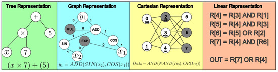
Figure 1.
Different AP representations for the generation of mathematical expressions.
DSRegPSOP applies a string transformation defined as for (the position of every particle of the particles and dimensions) to generate , with linear mathematical representations; each one is contained in a register ; i.e., for all the particles the transformation is , with as the total number of characters in each . Every is an equation that depends on previous registers, with the final output equation being the last register (). In Figure 2, a visual representation is presented, showcasing the spatial distribution of 100 particles, each characterized by 38 dimensions. Furthermore, the figure displays the equation and surface pertaining to the best particle in that iteration. This particle has two equation registers, i.e., .
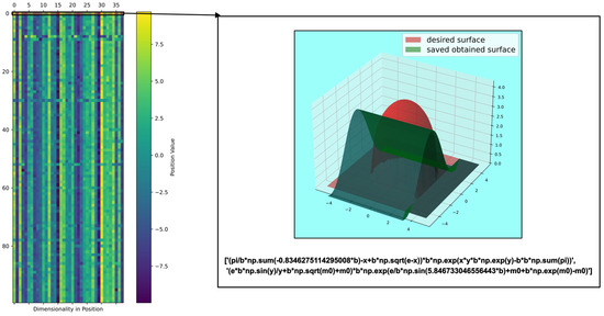
Figure 2.
Position of particles for generation of mathematical expressions in AP.
The complexity of a mathematical expression in a DSRegPSOP depends on several factors, including the operators, coefficients, variables, groups, and levels. These elements can be affected if a model is well-fitted and sub- or over-parameterized.
The coefficients (, , , , and ) and variables (, , and ) use operators like , , , , , , and , , , among others, in the mathematical expressions. Groups are sets of operations enclosed in parentheses and separated by operators. Each group forms a mathematical expression with operators, coefficients, and variables. The mathematical expressions have levels—the registers containing mathematical expressions with groups, every group with variables and coefficients, and operators. The output model is the final function in the last level () that depends on previous registers, like in Figure 3 with , , , and .

Figure 3.
Example of mathematical expression generated with DSRegPSOP.
The dimensionality required for the position of particles relies on the number of operators (), coefficients and variables (), groups (), and levels () according to Equation (1).
To convert the particle’s position into equations, we transform the position into two integer matrices (). One matrix contains all the particles of the indexes for operators (), and the other one includes the variables and coefficients (). Equations (2) and (3) allow for obtaining those indexes for every particle. These matrices are the indexes that allow re-mapping of the particle’s position to the corresponding operators saved in or the variables saved in .
where is the number of positions in the list of variables for coefficients. Given that each variable has an equal probability of being selected (i.e., there is one space in the list for each variable), this approach enables the control of the number of positions that are allocated to a numeric coefficient.
After obtaining and , adds the corresponding or depending on whether the dimension is a pair, the assignation takes the index from for odds and for pairs. Thus, each group in the equation has dimensions. The groups are delimited by parentheses and operators determined by the particles’ positions. Then, every level uses dimensions of containing groups. However, increases with every new , since it adds the variable that represents the previous register; thus, is re-calculated.
When the index of variables is greater than its number () a numerical coefficient is determined instead of a variable. Then, for that dimension, Equations (4) and (5) obtain the lower () and the upper () limits for re-mapping the coefficient to the search space range . Equation (6) obtains the numerical coefficient ().
Where and are the search space limits in the variant of the PSO algorithm, particularly in this work, DSRegPSO.
Finally, for every particle, each level is added to —the mathematical model for prediction or regression represented with the position of the particle.
The transformation proposed required for the DSRegPSOP is in Algorithm 1.
| Algorithm 1 Transformation |
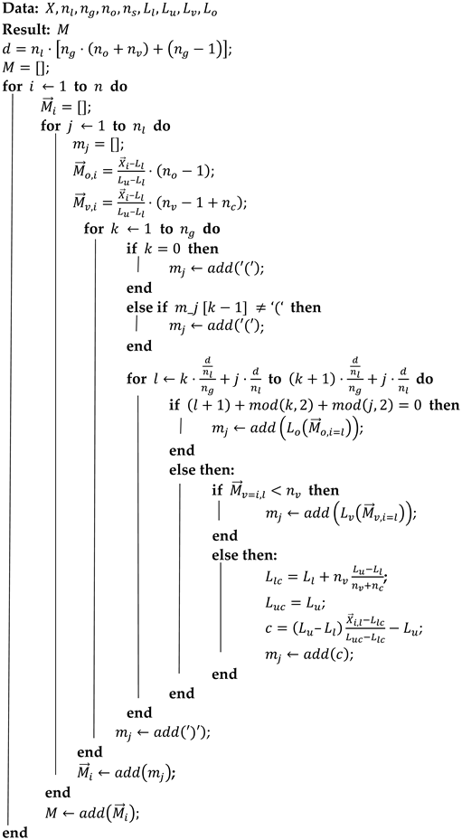 |
2.2. Particle Swarm Optimization with Inertial Coefficient (GPSO)
The PSO algorithm randomly initializes a numeric array of positions with where is the number of particles and is the search space dimensionality. Every iteration is updated depending on the speed array . The updating equations depend on the PSO version. In GPSO, the most utilized PSO with an inertial coefficient was proposed in 1998. The updating equations for speed and position are in Equations (7) and (8), respectively [39].
where is the inertial coefficient in ranges of as in the original algorithm [29]. and are personal and social coefficients, and their values are typically set to 2. is the global best position known, and is the best position known for each particle. and are random arrays in ranges with size . The position is updated every iteration using Equation (8) while being constrained within the lower position limit () and the upper position limit () [33,39].
Through multiple iterations of updating and using Equations (7) and (8) depending on a cost function , is drawn towards . Algorithm 2 describes the implementation of PSO with an inertial coefficient as in [39].
| Algorithm 2 GPSO |
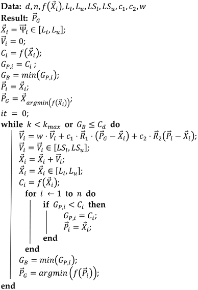 |
2.3. Dynamical Sphere Regrouping Particle Swarm Optimization (DSRegPSO)
DSRegPSO algorithm is a variant of PSO, inspired by PSO by bird flocking or fish schooling. In both algorithms, birds search for the best food source (best cost known) in a defined area (search space). During the search, birds adjust their position by following the current best-known position or the one nearest to the food. However, DSRegPSO introduces the situation of birds exhausting food when there is no improvement in the global best cost, forcing particles to travel to other locations to explore the search space while changing their speed and inertial behavior (dynamical sphere behavior). Additionally, DSRegPSO considers the physical principle of conservation momentum when the particles cross the frontier of the search space, as detailed in [33].
The DSRegPSO starts by obtaining the with Equation (9), which distributes the maximum inertial momentum () across and that control the inertial effect [33].
The speed of DSRegPSO is in Equation (10). It has three components: inertial , social , and personal . The inertial component contains the dynamical sphere regrouping mechanism controlled by the hyper-sphere diameter and its expansion speed . Social and personal components are the same as in the original PSO [33].
The speed limits in change across iterations. is the upper speed limit, and is the lower speed limit. They are initialized depending on the initial upper speed limit (). As in Equations (11)–(13) [33].
where is a coefficient that allows for the modification of the starting speed limits depending on the size of the search space.
After obtaining of the particle and retaining them under its limits, Equation (14) updates its position [33].
is a random array with positions between the lower position limit () and the upper position limit (). changes the position of particles too near to , based on that depends on the hyper-sphere diameter , as in Equation (15).
The distance is determined with Equation (16).
The sphere diameter is updated using Equation (17) if there is insufficient improvement () in global best cost (), i.e., . Similarly, obtains its value according to Equation (18). When there is enough improvement, and to maximize exploitation.
The conservation of momentum of DSRegPSO in Equation (19) maximizes exploration by returning particles to different positions in an opposite direction if the speed takes them beyond the search space boundaries.
and vary depending on , progressively reducing the size of the search space around the best position across iterations. The speed of refinement is controlled with and , as in Equations (20) and (21).
Finally, Equations (22) and (23) update the speed limits for each iteration while reaching the desired number of iterations () or a desired cost value ().
The DSRegPSO implementation is presented in Algorithm 3.
| Algorithm 3 DSRegPSO |
| Data: Result: ; ; ; ; ; ; ; ; ; ; ; ; ; ; ; ; 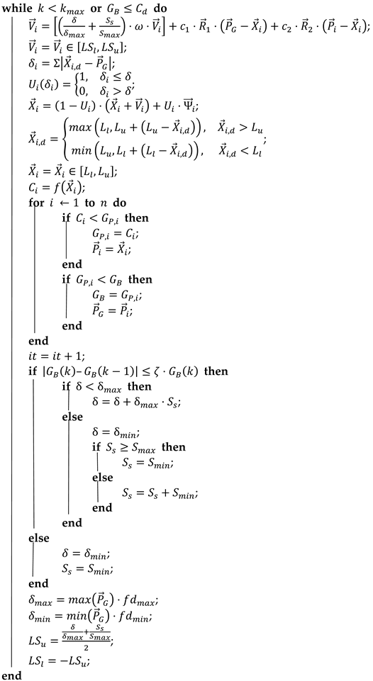 |
2.4. Dynamical Sphere Regrouping Particle Swarm Optimization Programming (DSRegPSOP)
Our proposed algorithm, DSRegPSOP, incorporates stagnation avoidance from DSRegPSO by utilizing dynamical sphere regrouping and conservation momentum mechanisms. These mechanisms work together to allow constant reinvigoration of the swarm. Dynamical sphere regrouping updates the positions of particles too near to the global best-known position or inside a sphere of diameter delta with the center as the global best-known position, and conservation momentum returns particles in the opposite direction when they travel away from the search space, as detailed in [33].
DSRegPSOP initializes with the same parameters required by DSRegPSO but is adapted to optimize the transformation of each particle with as detailed in Algorithm 1 to produce a desired equation. Thus, there are two parameters specifically defined for DSRegPSOP.
or number of dimensions in DSRegPSO is the first parameter determined with Equation (1) according to in Section 2.1.
The second parameter is the cost function, which for DSRegPSOP is depending on obtained with . is the Mean Square Error (MSE) between and , the desired and obtained responses of the generated equations, respectively. Moreover, we add two penalties to MSE as in Equation (24).
penalizes with gain the absolute distance between the maximum and minimum values of , like in Equation (25).
penalizes with gain the number of times that a previous register is not in the current register. This forces the model to use previous registers in each register, like in Equation (26).
verifies for each register if the previous ones are in it, like in Equation (27).
Algorithm 4 shows the implementation of the proposed DSRegPSOP to obtain an optimized model for regression, classification, or prediction.
| Algorithm 4 DSRegPSOP |
| Data: Result: ; ; ; ; ; ; ; ; ; ; ; ; ; ; ; ; ; 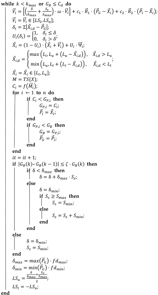 |
2.5. Evaluation and Comparison Benchmarks
We evaluate the performance of DSRegPSOP using datasets. Many researchers have assessed their algorithms using datasets for symbolic regression tasks, but there is currently no standardized framework for benchmarking these problems [46]. Some examples of repositories with datasets for regression and classification tasks are UC machine learning [47], Kaggle [48], and PMLB [49]. Alternatively, SRbench is a framework designed for benchmarking symbolic regression algorithms. It’s important to note that this framework isn’t a standardized benchmark but rather a tool for testing algorithms using datasets already published in other repositories [50].
In this work, we evaluate the DSRegPSOP with datasets of real-world problems. The datasets chosen for testing DSRegPSOP were selected based on their popularity of benchmarking symbolic regression and the existence of documented results in the literature for the purpose of comparison. The datasets used are
- Airfoil: A 1989 dataset of NASA for prediction of noise in aerodynamic and acoustic tests of two and three-dimensional airfoil blade sections conducted in an anechoic wind tunnel. The dataset contains the features of frequency, angle of attack, chord length, free stream velocity, suction side displacement thickness, and scaled sound pressure level; this last is the variable to predict [51,52].
- Concrete: A 1998 dataset that allows for the prediction of concrete strength based on amounts of cement, slag from blast furnaces, fly ash, water, superplasticizer, coarse aggregate, fine aggregate, age of the concrete in days (1–365), and concrete compressive strength; this last one is the target variable [53].
- Energy: A dataset of 2012 for the prediction of cooling and heating requirements for buildings with input features including relative compactness, surface area, wall area, roof area, overall height, orientation, glazing area, and glazing area distribution [54,55]. In this work, we focus on the prediction of cooling load for the third dataset test.
- Yacht: Is a 2013 dataset to predict the hydrodynamic performance of sailing yachts based on the longitudinal position of the center of buoyancy, prismatic coefficient, length-displacement ratio, beam-draught ratio, length-beam ratio, Froude number, residuary resistance per unit weight of displacement, this last one is the target variable [56].
- Geographical Origin of Music: A 2014 dataset with audio features extracted from 1059. The goal is to predict the geographical origin of the track. The input features are 68 numerical values extracted from the music with the Music Analysis, Retrieval, and Synthesis for Audio Signals framework (MARSYAS) [57,58]. In this work, we focus only on the latitude related to music, as detailed in [59].
- Tecator: A 2006 dataset with data of the spectrum recorded on a food and feed analyzer working in the wavelength range 850–1050 nm by the near-infrared transmission principle. Each sample contains meat with different moisture, fat, and protein contents [60].
Additionally, we value DSRegPSOP with a proposed benchmark that includes 10 tests; each one uses known equations with two-dimensional functions that generate three-dimensional surfaces. Moreover, all of them have two dependent variables, and , that produce a surface in . Thus, the DSRegPSO must optimize a model for the target surface generated in . The data is not split to optimize the equation and represent the target surface using the same information points as in numerical optimization benchmarks. In this work, we are dealing with three-dimensional surfaces, but the functions can exhibit increased dimensionality, like in numerical optimization benchmarks [61].
Analyzing three-dimensional surfaces enables the assessment of DSRegPSOP with visually represented data in a three-dimensional format. Nonetheless, we are still using the most common regression metrics for comparative purposes, including Mean Absolute Error (MAE), Mean Absolute Percentage Error (MAPE), Mean Square Error (MSE), and R-square () [33]. Moreover, as in other benchmarks, we evaluate the quality of results by adding noise to the cost function and the position of particles.
The 10 functions in the proposed benchmark for testing DSRegPSOP are
Function 1: This is the simplest test in the benchmark and includes a second-degree polynomial with a trigonometric function. The dependent variables in ranges and with 20 points per variable, i.e., 400 points for . The different ranges for dependent variables simplify distinguishing between them. Equation (28) shows function 1, and Figure 4 shows its surface.
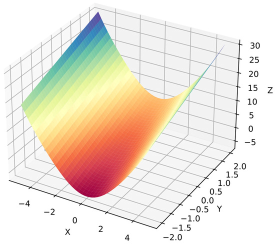
Figure 4.
Surface of function 1.
Function 2: A sphere function is common in numerical optimization benchmarks [62] but it is a more complex problem in symbolic regression because the algorithm must optimize the equation to obtain the target surface. Now the algorithm cannot distinguish between dependent variables because they are in similar ranges with 40 points per variable, i.e., 1600 points for . Equation (29) shows function 2, and Figure 5 shows its surface.
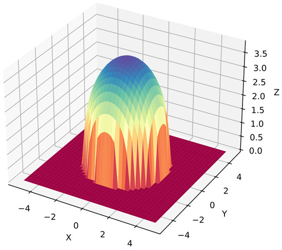
Figure 5.
Surface of function 2.
Function 3: The Rastrigin function is also common in numerical optimization benchmarks [62], but it is a more complex problem in symbolic regression because the algorithm must optimize the equation for the target surface. Moreover, the algorithm cannot distinguish dependent variables since they are in similar ranges with 40 points per variable, i.e., 1600 points for . Equation (30) shows function 3, and Figure 6 shows its surface.
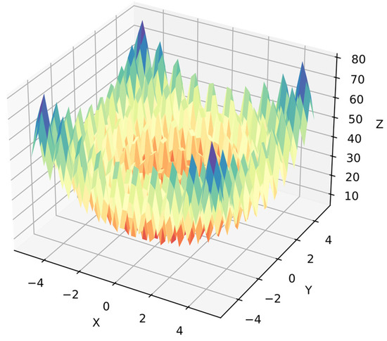
Figure 6.
Surface of function 3.
Function 4: The Ackley function is also common in numerical optimization benchmarks [62], but it is a more complex problem in symbolic regression because the algorithm must optimize the equation for the target surface. Moreover, the algorithm cannot distinguish dependent variables since they are in similar ranges with 40 points per variable, i.e., 1600 points for . Equation (31) shows function 4, and Figure 7 shows its surface.
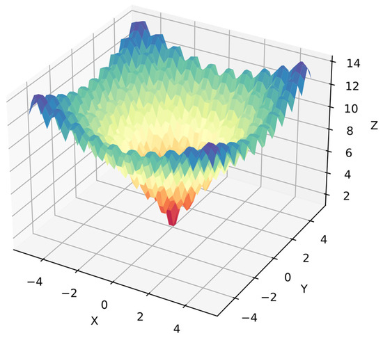
Figure 7.
Surface of function 4.
Function 5: This is a trigonometric function with multiple dependent variables in its argument. Furthermore, the algorithm cannot distinguish dependent variables, and this time, the search space is bigger compared with previous functions. Moreover, there are fewer information points since the dependent variables are in ranges with 20 points per variable, i.e., 400 points for . Equation (32) shows function 5, and Figure 8 shows its surface.
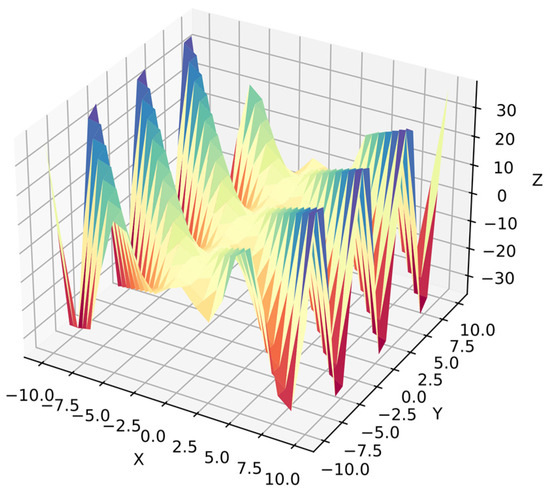
Figure 8.
Surface of function 5.
Function 6: This is an exponential function with multiple dependent variables in its argument. Again, the algorithm cannot distinguish dependent variables. However, the search space is smaller in ranges because the exponential function produces bigger values, and there is less information than in the simpler functions since there are 20 points per variable, i.e., 400 points for . Equation (33) shows function 6, and Figure 9 shows its surface.
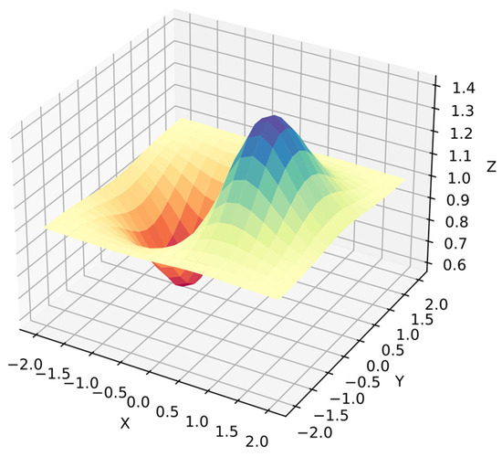
Figure 9.
Surface of function 6.
Function 7: This is a hyperbolic paraboloid function with fractions and quadratic terms for each dependent variable. Again, the search space is bigger than in the simpler functions, and the algorithm cannot distinguish between dependent variables in ranges . Similarly, there is less information than in the simpler functions since there are 20 points per variable, i.e., 400 points for . Equation (34) shows function 7, and Figure 10 shows its surface.
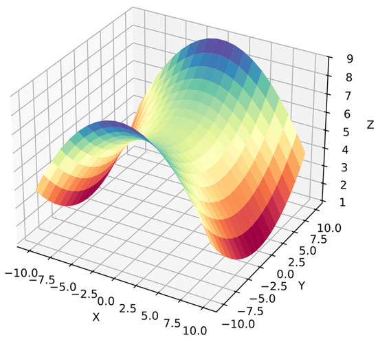
Figure 10.
Surface of function 7.
Function 8: The Rosenbrock function has sharp peaks and regions with values near zero. It is also common in numerical optimization benchmarks [62], but it is a more complex problem in symbolic regression because the algorithm must optimize the equation for the target surface. Moreover, the algorithm cannot distinguish dependent variables since they are in similar ranges . The search space has less information than in simpler functions with 20 points per variable, i.e., 400 points for . Equation (35) shows function 8, and Figure 11 shows its surface.

Figure 11.
Surface of function 8.
Function 9: The Beale function has sharp peaks and regions with values near zero. The Beale function is also common in numerical optimization benchmarks [62], but it is a more complex problem in symbolic regression because the algorithm must optimize the equation for the target surface. Moreover, the algorithm cannot distinguish dependent variables since they are in similar ranges . The search space has less information than simpler functions with 20 points per variable, i.e., 400 points in . Equation (36) shows function 9, and Figure 12 shows its surface.
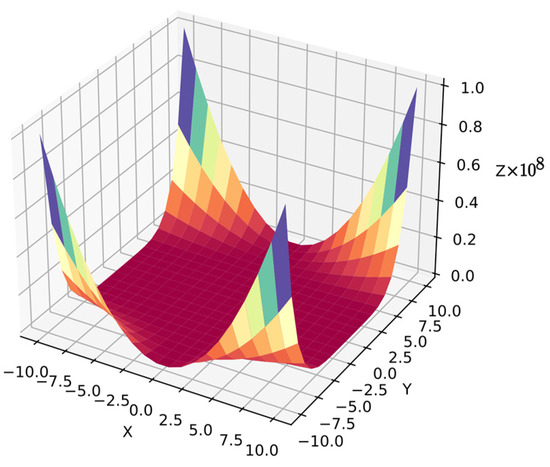
Figure 12.
Surface of function 9.
Function 10: The Goldstein-Price function has sharp peaks and several local minimal regions. Goldstein-Price function is also common in numerical optimization benchmarks [62], but it is a more complex problem in symbolic regression because the algorithm must optimize the equation for the target surface. Moreover, the algorithm cannot distinguish dependent variables since they are in similar ranges . The search space has less information than simpler functions with 20 points per variable, i.e., 400 points for . Equation (37) shows function 10, and Figure 13 shows its surface.

Figure 13.
Surface of function 10.
3. Results and Discussion
The results and experiments were carried out on a computer running Microsoft Windows 11 Pro with a 10.0.22631-core 12th Gen Intel(R) Core (TM) i5-12400F processor, operating at 2500 Mhz. The system was equipped with 6 main cores, 12 logical cores, and 64.0 GB of RAM, and Python version 3.9.10 was used for all computations, without utilizing parallel computing.
3.1. Results in Benchmark with Three-Dimensional Functions
3.1.1. Experimental Setup of Benchmark in Three-Dimensional Functions
All the functions in this benchmark have the same considerations:
- The maximum number of function evaluations for each test is , but it could be less during hyperparameter tuning due to the next point.
- During hyperparameter tunning, the test is stopped, and the result is recorded if best cost value reaches .
- The list of variables is.
- The list of operators is.
- The DSRegPSOP static parameters for all the functions are
- The parameters that are dependent on the optimized function are
- The and parameters are adapted so that and in the first iteration.
- The and are specified according to the search space limits in the test function.
- The , , and parameters are obtained with exhaustive search exploring the 64 combinations produced with: , , and .
- There is no data split since the goal of this test is to optimize the surface as much as possible with the information points in the target surface.After finding the best configuration with an exhaustive search, the algorithm trains again but without stopping if the cost reaches value.
- After finding the best configuration with an exhaustive search, the algorithm trains again but adds 0–25% noise in the cost function and position of particles to test the robustness of the algorithm.
3.1.2. Results Function 1
The best solution found in an exhaustive search for function 1 was with , and obtaining the best metrics , , , , and , which support that DSRegPSOP successfully optimized the target surface. The top 10 configurations are in Table 1, and Figure 14 shows the parallel plot with the results of all the configurations used.

Table 1.
Top 10 exhaustive search results testing function 1.
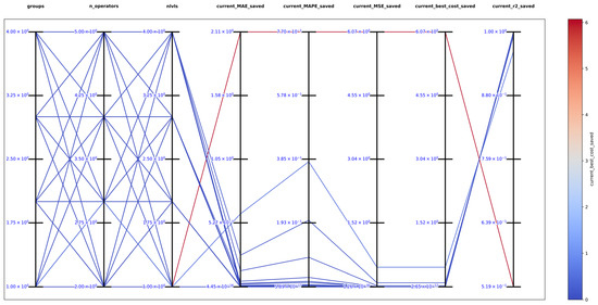
Figure 14.
Parallel plot of hyperparameters for exhaustive search in function 1.
Figure 15 shows the comparison of the best obtained and target surface, including the heatmap and principal component analysis, reduced to three dimensions to show the positions of particles in the last iteration. Furthermore, the particles could still improve since the DSRegPSOP algorithm never converges and still explores the search space as DSRegPSO does.
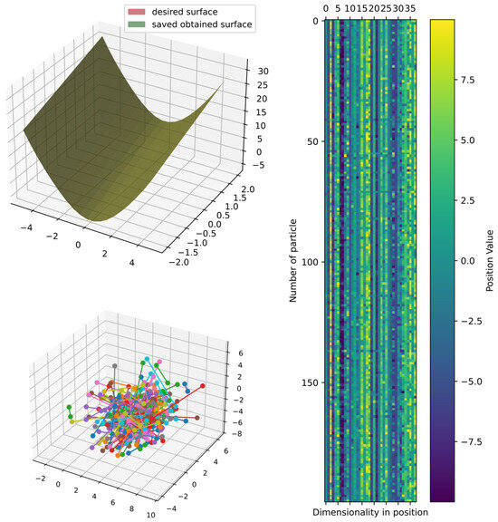
Figure 15.
Comparison of obtained and target surface showing PCA with random color for each of the 200 particles and heatmap for the position of particles from to function evaluations for function 1.
Additionally, we assess DSRegPSOP for noise effect in position and cost evaluation with ranges 0–25% in function 1. The results in Table 2 show a minimal variation in best cost and . Moreover, the minimal variation with noise is also evident in the convergence diagram in Figure 16.
Table 2.
Effects of noise in position and cost evaluation for function 1.

Figure 16.
Effects of noise in position and cost evaluation for function 1.
3.1.3. Results Function 2
The best solution in an exhaustive search for function 2 was obtained with , and obtaining the best metrics , , , , and , which support that DSRegPSOP successfully optimized the target surface. The top 10 configurations are in Table 3, and Figure 17 shows the parallel plot with the results of all the configurations.
Table 3.
Top 10 exhaustive search results testing function 2.
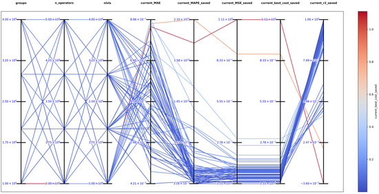
Figure 17.
Parallel plot of hyperparameters for exhaustive search in function 2.
Figure 18 shows the best model obtained compared with the target surface; the heatmap and principal component analysis were reduced to three dimensions to show the positions of particles. However, the best cost could still improve since the position of particles in the DSRegPSOP algorithm never converges due to the dynamical sphere regrouping behavior inherited from the DSRegPSO, which reinvigorates the swarm by assigning a new position to the particles positioned inside the sphere limited by the diameter according to Equation (14). Thus, DSRegPSOP remains exploring the search space, avoiding premature convergence.

Figure 18.
Comparison of obtained and target surface showing PCA with random color for each of the 200 particles and heatmap for the position of particles from to function evaluations for function 2.
Similarly, we evaluate DSRegPSOP for noise effect in position and cost evaluation with ranges 0–25% for function 2. The results in Table 4 show that the variation with noise is bigger than in function 1, but the variation is minimal if the noise is applied to the cost value. From the convergence diagram for noise evaluations in Figure 19, it is also evident that there is a bigger affectation with noise in position.
Table 4.
Effects of noise in position and cost evaluation for function 2.

Figure 19.
Effects of noise in position and cost evaluation for function 2.
3.1.4. Results Function 3
The best solution in an exhaustive search for function 3 was obtained with , and obtaining the best metrics , , , , and , which show that DSRegPSOP optimized the target surface, but the error is considerable based on .
The top 10 configurations are in Table 5, and Figure 20 shows the parallel plot with the results of all the configurations. Figure 21 also shows that the heatmap and principal component analysis are reduced to three dimensions to show the positions of particles in the last iteration.
Table 5.
Top 10 exhaustive search results testing function 3.
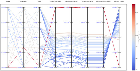
Figure 20.
Parallel plot of hyperparameters for exhaustive search in function 3.
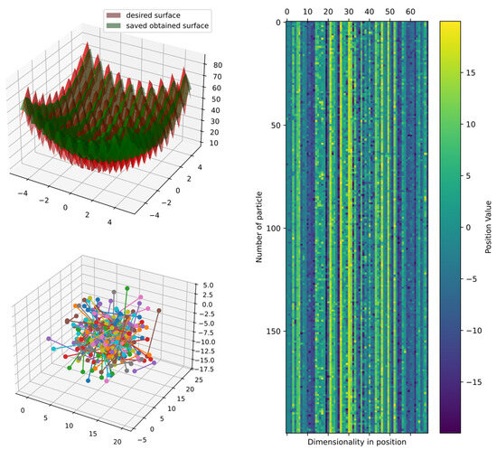
Figure 21.
Comparison of obtained and target surface showing PCA with random color for each of the 200 particles and heatmap for the position of particles from to function evaluations for function 3.
Despite the error in for function 3, based on the comparison with the target and obtained surfaces in Figure 21, we found that the two surfaces are similar in the prediction, but the obtained surface cannot mimic the natural noise in function 3. However, the particles could still improve since the DSRegPSOP algorithm never converges and is still exploring the search space as DSRegPSO does.
Similarly, we evaluate DSRegPSOP for noise effect in position and cost evaluation with ranges 0–25% for function 3. The results in Table 6 show that the variation with noise is bigger than in previous functions, and this time, the noise also affects the cost value. The convergence diagram for noise evaluations in Figure 22 shows that the error increases with both noises, but the noise in position affects more than in cost value.
Table 6.
Effects of noise in position and cost evaluation for function 3.
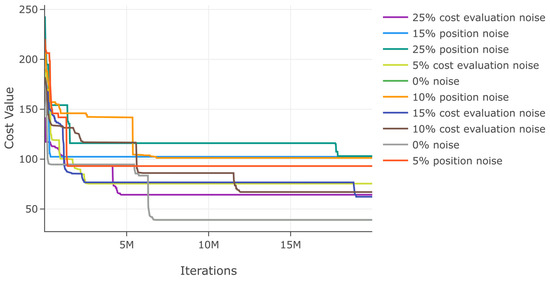
Figure 22.
Effects of noise in position and cost evaluation for function 3.
3.1.5. Results Function 4
The best solution in an exhaustive search for function 4 was obtained with , and obtaining the best metrics , , , , and , which show that DSRegPSOP optimized the target surface, but the error is considerable based on .
The top 10 configurations are in Table 7 and Figure 23 shows the parallel plot with the results of all the configurations tested. Figure 23 also shows the heatmap and principal component analysis reduced to three dimensions to show the positions of particles in the last iteration.
Table 7.
Top 10 exhaustive search results testing function 4.
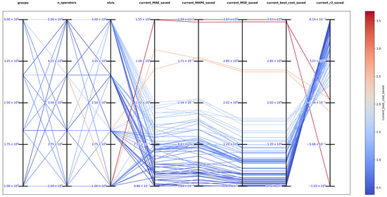
Figure 23.
Parallel plot of hyperparameters for exhaustive search in function 4.
Despite the error in for function 4, based on the comparison with the target and obtained surfaces in Figure 24, we found that the two surfaces are similar in general prediction, but the obtained surface cannot mimic the natural noise in function 4. However, the particles could still improve since the DSRegPSOP algorithm never converges and is still exploring the search space as DSRegPSO does.

Figure 24.
Comparison of obtained and target surface showing PCA with random color for each of the 200 particles and heatmap for the position of particles from to function evaluations for function 4.
Similarly, we assess DSRegPSOP for noise effect in position and cost evaluation with ranges 0–25% for function 4. The results in Table 8 show that the variation with noise is bigger than in functions 1 and 2 but lower than in 3. The convergence diagram for noise evaluations is in Figure 25 shows that there is affectation with both noises, but the noise in position affects more than in cost value.
Table 8.
Effects of noise in position and cost evaluation for function 4.
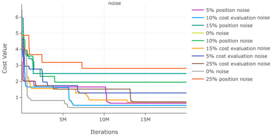
Figure 25.
Effects of noise in position and cost evaluation for function 4.
3.1.6. Results Function 5
The best solution in an exhaustive search for function 5 was obtained with , and obtaining the best metrics , , , , and , which show that DSRegPSOP successfully optimized the target surface based on . The top 10 configurations are in Table 9, and Figure 26 shows the parallel plot with the results of all the configurations tested.
Table 9.
Top 10 exhaustive search results testing function 5.
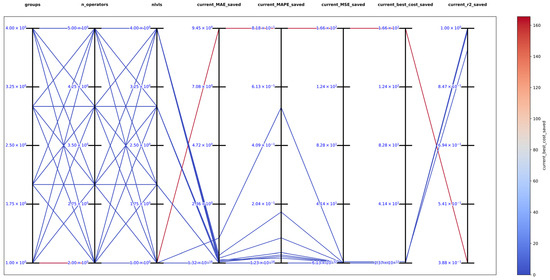
Figure 26.
Parallel plot of hyperparameters for exhaustive search in function 5.
Figure 27 shows the comparison of the best obtained and target surface, including the heatmap and principal component analysis, which are reduced to three dimensions to show the positions of particles in the last iteration. Furthermore, the particles could still improve since the DSRegPSOP algorithm never converges and is still exploring the search space as DSRegPSO does.
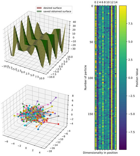
Figure 27.
Comparison of obtained and target surface showing PCA with random color for each of the 200 particles and heatmap for the position of particles from to function evaluations for function 5.
Again, we evaluate DSRegPSOP for noise effect in position and cost evaluation with ranges 0–25% in function 5. The results in Table 10 show a minimal variation in best cost and . Moreover, the minimal variation with noise is also evident in the convergence diagram in Figure 28.
Table 10.
Effects of noise in position and cost evaluation for function 5.
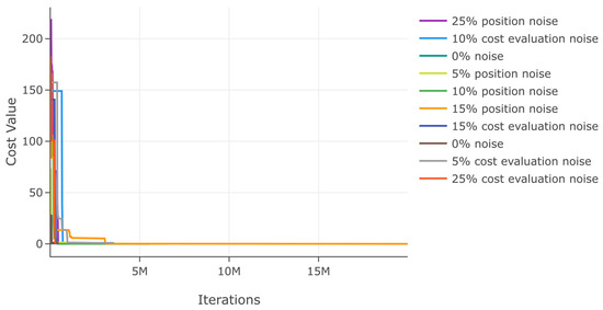
Figure 28.
Effects of noise in position and cost evaluation for function 5.
3.1.7. Results Function 6
The best solution in an exhaustive search for function 6 was obtained with , and obtaining the best metrics , , , , and , which show that DSRegPSOP successfully optimized the target surface based on . The top 10 configurations are in Table 11, and Figure 29 shows the parallel plot with the results of all the configurations tested.
Table 11.
Top 10 exhaustive search results testing function 6.
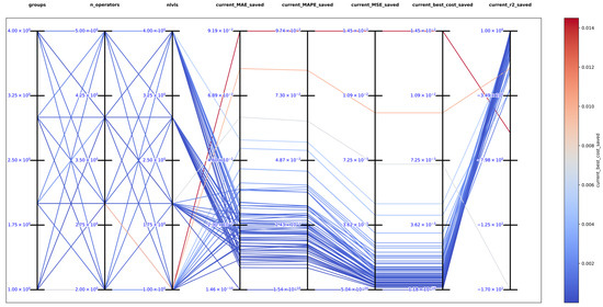
Figure 29.
Parallel plot of hyperparameters for exhaustive search in function 6.
Figure 30 shows the comparison of the obtained and target surface, including the heatmap and principal component analysis, which are reduced to three dimensions for visualizing the positions of particles in the last iteration. Furthermore, the particles could still improve since the DSRegPSOP algorithm never converges and is still exploring the search space as DSRegPSO does.

Figure 30.
Comparison of obtained and target surface showing PCA with random color for each of the 200 particles and heatmap for the position of particles from to function evaluations for function 6.
Similarly, we evaluate DSRegPSOP for noise effect in position and cost evaluation with ranges 0–25% for function 6. The results in Table 12 show that the variation with noise is bigger than in functions 1 and 2 but lower than in 3. The convergence diagram for noise evaluations is in Figure 31, which shows that there is affectation with both noises, but the noise in position affects more than in cost value.
Table 12.
Effects of noise in position and cost evaluation for function 6.
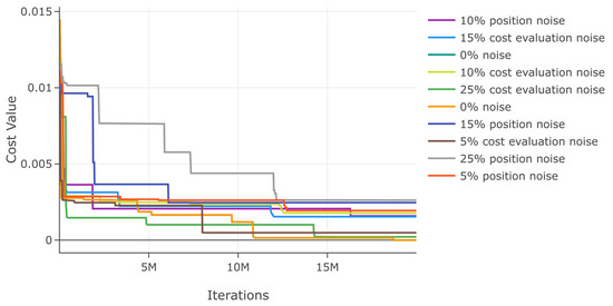
Figure 31.
Effects of noise in position and cost evaluation for function 6.
3.1.8. Results Function 7
The best solution in an exhaustive search for function 7 was obtained with , and obtaining the best metrics , , , , and , which show that DSRegPSOP successfully optimized the target surface based on . The top 10 configurations are in Table 13, and Figure 32 shows the parallel plot with the results of all the configurations tested.
Table 13.
Top 10 exhaustive search results testing function 7.
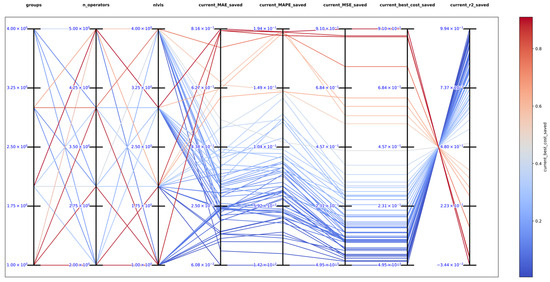
Figure 32.
Parallel plot of hyperparameters for exhaustive search in function 7.
Figure 33 shows the comparison of the best obtained and target surface, including the heatmap and principal component analysis, which are reduced to three dimensions to show the positions of particles in the last iteration. Furthermore, the particles could still improve since the DSRegPSOP algorithm never converges and is still exploring the search space as DSRegPSO does.

Figure 33.
Comparison of obtained and target surface showing PCA with random color for each of the 200 particles and heatmap for the position of particles from to function evaluations for function 7.
Similarly, we evaluate DSRegPSOP for noise effect in position and cost evaluation with ranges 0–25% for function 7. The results in Table 14 show that the variation with noise is bigger than in functions 1 and 2 but lower than in 3. The convergence diagram for noise evaluations is in Figure 34; it shows that there is affectation with both noises, but the noise in position affects more than in cost value.
Table 14.
Effects of noise in position and cost evaluation for function 7.
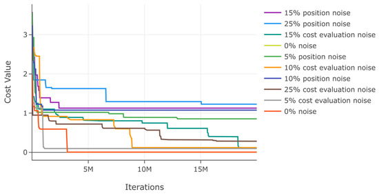
Figure 34.
Effects of noise in position and cost evaluation for function 7.
3.1.9. Results Function 8
The best solution in an exhaustive search for function 8 was obtained with , and obtaining the best metrics , , , , and , which show that DSRegPSOP successfully optimized the target surface based on . The top 10 configurations are in Table 15, and Figure 35 shows the parallel plot with the results of all the configurations tested.
Table 15.
Top 10 exhaustive search results testing function 8.
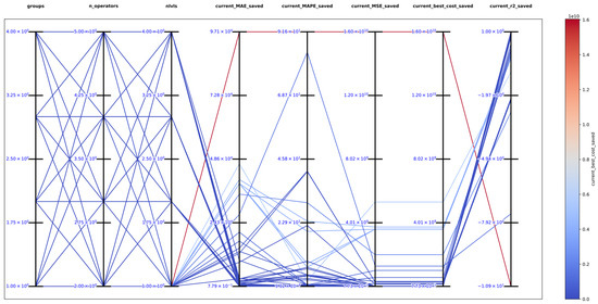
Figure 35.
Parallel plot of hyperparameters for exhaustive search in function 8.
Figure 36 shows the comparison of the best obtained and target surface, including the heatmap and principal component analysis, which are reduced to three dimensions to show the positions of particles in the last iteration. Furthermore, the particles could still improve since the DSRegPSOP algorithm never converges and is still exploring the search space as DSRegPSO does.

Figure 36.
Comparison of obtained and target surface showing PCA with random color for each of the 200 particles and heatmap for the position of particles from to function evaluations for function 8.
Similarly, we evaluate DSRegPSOP for noise effect in position and cost evaluation with ranges 0–25% for function 8. The results in Table 16 show that the variation with noise is minimal and reaches its maximum error at 25% of noise in position. The convergence diagram for noise evaluations is in Figure 37; it shows that there is minimal affectation with both noises, but the noise in position affects when it reaches 25% of noise.
Table 16.
Effects of noise in position and cost evaluation for function 8.
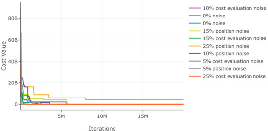
Figure 37.
Effects of noise in position and cost evaluation for function 8.
3.1.10. Results Function 9
The best solution in an exhaustive search for function 9 was obtained with , and obtaining the best metrics , , , , and , which show that DSRegPSOP successfully optimized the target surface based on . The top 10 configurations are in Table 17, and Figure 38 shows the parallel plot with the results of all the configurations tested.
Table 17.
Top 10 exhaustive search results testing function 9.
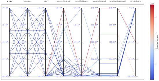
Figure 38.
Parallel plot of hyperparameters for exhaustive search in function 9.
Figure 39 shows the comparison of the obtained and target surface, including the heatmap and principal component analysis, which are reduced to three dimensions to show the positions of particles in the last iteration. Furthermore, the particles could still improve since the DSRegPSOP algorithm never converges and is still exploring the search space as DSRegPSO does.
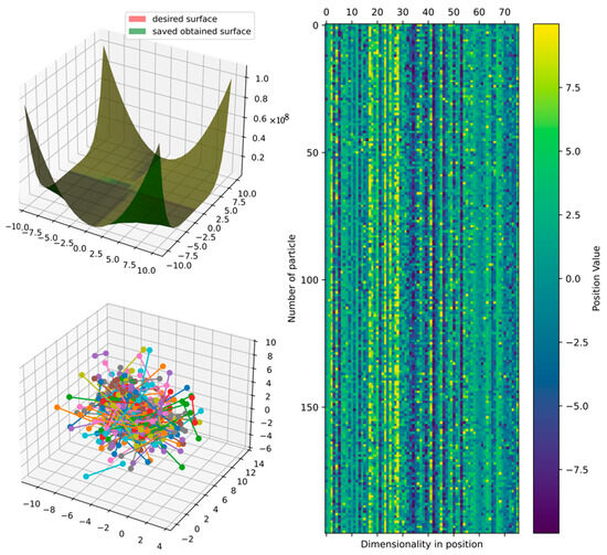
Figure 39.
Comparison of obtained and target surface showing PCA with random color for each of the 200 particles and heatmap for the position of particles from to function evaluations for function 9.
Again, we evaluate DSRegPSOP for noise effect in position and cost evaluation with ranges 0–25% in function 9. The results in Table 18 show a minimal variation in best cost and . Moreover, the minimal variation with noise is also evident in the convergence diagram in Figure 40.
Table 18.
Effects of noise in position and cost evaluation for function 9.
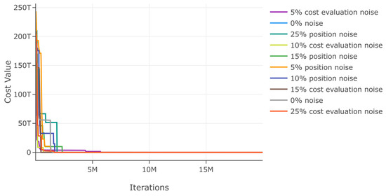
Figure 40.
Effects of noise in position and cost evaluation for function 9.
3.1.11. Results Function 10
The best solution in an exhaustive search for function 10 was obtained with , and obtaining the best metrics , , , , and , which show that DSRegPSOP successfully optimized the target surface based on . The top 10 configurations are in Table 19, and Figure 41 shows the parallel plot with the results of all the configurations tested.
Table 19.
Top 10 exhaustive search results testing function 10.
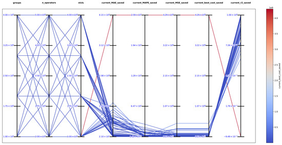
Figure 41.
Parallel plot of hyperparameters for exhaustive search in function 10.
Figure 42 shows the comparison of the best obtained and target surface, including the heatmap and principal component analysis, which are reduced to three dimensions to show the positions of particles in the last iteration. Furthermore, the particles could still improve since the DSRegPSOP algorithm never converges and is still exploring the search space as DSRegPSO does.
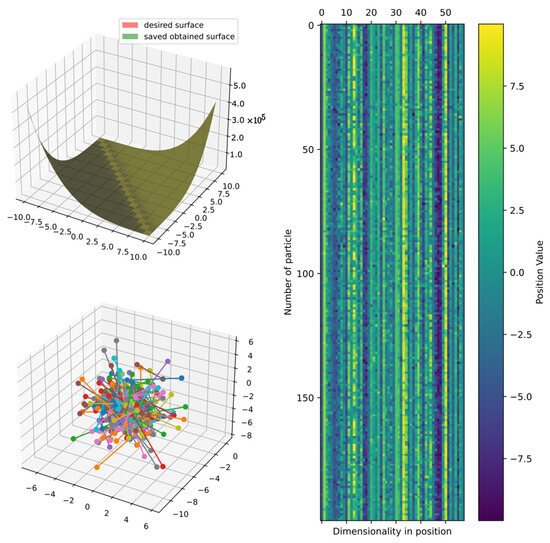
Figure 42.
Comparison of obtained and target surface showing PCA with random color for each of the 200 particles and heatmap for the position of particles from to function evaluations for function 10.
Similarly, we test DSRegPSOP for noise effect in position and cost evaluation with ranges 0–25% for function 10. The results in Table 20 show that the variation with noise is minimal and reaches its maximum error at 25% of noise in position. The convergence diagram for noise evaluations is in Figure 43; it shows that there is minimal affectation with both noises, but the noise in position affects more than in cost value.
Table 20.
Effects of noise in position and cost evaluation for function 10.

Figure 43.
Effects of noise in position and cost evaluation for function 10.
3.2. Results in Benchmark with Datasets
3.2.1. Experimental Setup of Benchmark with Datasets
All the datasets in this benchmark have the same considerations:
- We split datasets into 80% for training and 20% for testing and performing six-fold cross-validation.
- The maximum number of function evaluations for each dataset is to compare with several algorithms in the first stage of optimization described in [63].
- During hyperparameter tunning, the test stops, and the result is recorded if the cost value reaches .
- The list of variables is:.
- The list of operators is:.
- The DSRegPSOP static parameters for all the functions are:
We chose to demonstrate the capabilities of DSRegPSOP by optimizing with only five particles. This number was sufficient for the datasets we used. However, for the more complex initial benchmark involving surfaces, we needed to increase for effective optimization.
- The parameters that are dependent on the optimized dataset are:and
- The and parameters are adapted for each function so that:and in the first iteration.
- The , , and parameters are obtained with an exhaustive search exploring the 64 combinations produced with: , , and .
- Again, we perform a hyperparameter tuning with 64 configurations and six-fold cross-validation, as before, but we also perform running/function evaluations to compare the DSRegPSOP results with those in the literature for each dataset.
- All the generated models for dataset prediction apply the RELU activation function at the final register or the maximum across the evaluation and zero value. This has shown improved results in regression tasks with ANNs, and we found DSRegPSOP benefits of it.
3.2.2. Results in Datasets Benchmark
Table 21 shows the mean RMSE and standard deviation obtained with the function evaluations for the training stage in the six-fold cross-validation for regression in the real-world datasets. These results allow the comparison with other algorithms described in [63]. DSRegPSOP is not the best solution, which is understandable with function evaluations when the equation is generated with metaheuristic algorithms with AP approaches. However, it is better than at least one of the variants of GP (dcGP, GP, or GSGP) in five of the six datasets. Moreover, with more function evaluations, DSRegPSOP obtains competitive results that are the best reported in the literature for each dataset.
Table 21.
Comparison of algorithms with DSRegPSOP training RMSE and standard deviation with benchmark datasets.
Table 22 shows the mean RMSE and standard deviation obtained with the function evaluations for the testing stage in the six-fold cross-validation for regression in the real-world datasets. Again, DSRegPSOP is not the best solution. However, it is better than GP in eight of the nine datasets. Moreover, with more function evaluations, DSRegPSOP obtains competitive results that are the best reported in the literature for each dataset.
Table 22.
Comparison of algorithms with DSRegPSOP testing RMSE and standard deviation with benchmark datasets.
After function evaluations in a time span of 1 h, 58 min, and 12 s, the DSRegPSOP obtains an RMSE and around the average of the best results obtained with algorithms that have been used for regression for predicting pressure with the Airfoil dataset (Table 23) [64,65]. However, it is the only one that produces a model entirely generated with AP approaches instead of tuning parameters in a human-proposed structure. The parameters for obtaining the best model in Equations (38) to (41) are , and .
Table 23.
Best results in the literature for regression with the Airfoil dataset.
Similarly, after function evaluations in a time span of 3 h, 10 min, and 47 s, the DSRegPSOP obtains the best RMSE and results compared with other algorithms that have been used for regression with the concrete strength dataset as detailed in Table 24 [66]. Moreover, DSRegPSOP is the only one that produces a model entirely generated with AP approaches instead of tuning parameters in a proposed structure. The parameters for obtaining the best model in Equations (42) to (44) are , , and .
Table 24.
Best results in the literature for regression with the Concrete dataset.
DSRegPSOP, after the function evaluations in a time span of 1 h, 33 min, and 31 s, obtains an RMSE and around the average of the best results obtained with algorithms that have been used for regression with the cooling load dataset in Table 25 [67]. However, it is the only one that produces a model entirely generated with AP approaches instead of tuning parameters in a human-proposed structure. The parameters for obtaining the best model in Equations (45) to (47) are , and
Table 25.
Best results in the literature for regression with Cooling Load dataset.
DSRegPSOP, after function evaluations in a time span of 1 h, 32 min, and 18 s, obtains an RMSE and around the average of the best results obtained with algorithms that have been used for regression in the prediction of sailing resistance in yachts as detailed in Table 26 [68,69]. However, it is the only one that produces a model entirely generated with AP approaches instead of tuning parameters in a human-proposed structure. The parameters for obtaining the best model in Equations (48) to (51) are , , and .
Table 26.
Best results in the literature for regression with yachts sailing resistance dataset.
DSRegPSOP obtains after function evaluations in a time span of 1 h, 51 min, and 32 s, an RMSE and around the average of the best results obtained with algorithms that have been used for regression in the prediction of geographical latitude based on music as detailed in Table 27 [57,59]. Moreover, DSRegPSOP is the only one that produces a model entirely generated with AP approaches instead of tuning parameters in a human-proposed structure. The parameters for obtaining the best model for latitude prediction in Equations (52) to (54) are , , and .
Table 27.
Best results in the literature for regression with geographical location dataset.
DSRegPSOP obtains after function evaluations in a time span of 2 h, 56 min, and 27 s, the best RMSE and obtained compared with algorithms that have been used for regression in the prediction of fat content of in a meat sample as detailed in Table 28 [70]. Moreover, DSRegPSOP is the only one that produces a model entirely generated with AP approaches instead of tuning parameters in a human-proposed structure. The parameters for obtaining the best model in Equations (55) to (57) are , , and .
Table 28.
Best results in the literature for regression with a prediction of fat in the Tecator dataset.
3.3. Statistical Proofing Comparing DSRegPSO against Other Algorithms
To assess the effectiveness of DSRegPSOP in comparison to various algorithms on different datasets, we conducted the Kruskal-Wallis test. This non-parametric test enables the comparison of multiple independent groups to ascertain whether they stem from the same distribution [71]. RMSE values allow the Kruskal-Wallis test to be obtained to pinpoint any noteworthy disparities in performance, as shown in Table 29.
Table 29.
Kruskal-Wallis Statistic Test.
The results clearly indicate that, in all datasets analyzed, the p-values from the Kruskal-Wallis test exceeded 0.05, demonstrating no significant differences in performance (measured by RMSE) among the compared algorithms. In essence, all algorithms demonstrated statistically similar performance across the datasets. This finding strongly supports the notion that our algorithm, DSRegPSOP, is competitive and performs comparably to other state-of-the-art algorithms in the evaluated datasets.
4. Conclusions
In this work, we introduce DSRegPSOP, an algorithm developed for automatic programming to address the limitations of PSO in PSP, which was constrained to theoretical applications as it was prone to stagnation in high-dimensional spaces with numerous local optimal regions like those in automatic programming search spaces.
DSRegPSOP focuses on avoiding stagnation in local optimal regions in high-dimensional spaces by thoroughly exploring the search space and reinvigorating the swarm using dynamical sphere regrouping and momentum conservation effects inherited from DSRegPSO.
The models created using DSRegPSOP effectively transform the particle positions into intricate model equations. This is achieved by generating sets of equations organized into multiple levels with various parentheses, operators, variables, and numeric coefficients, which are dependent on the particle positions.
We evaluated DSRegPSOP using two different methods. First, we created a benchmark with 10 complex surfaces in a three-dimensional space to visually assess the performance of DSRegPSOP while registering , MSE, MAE, and MAPE. These surfaces were similar to those used in numerical optimization tests such as the CEC’13 benchmark. We chose this approach because there is no universally accepted test for evaluating algorithms in symbolic regression. Our intention is for other researchers to compare their algorithms with DSRegPSOP using this first evaluation as a reference point.
We found in this test that DSRegPSOP successfully optimized 8 of the 10 functions with remarkable results with an near 1.0, and functions 3 and 4 being more complex registered and , respectively. However, the complexity of this test can be upscaled by increasing the search space dimensionality in each surface as it occurs in numerical optimization benchmarks.
The second evaluation method considers that algorithms in symbolic regression are assessed using diverse datasets. Therefore, our second approach tests and compares DSRegPSOP with other algorithms using six datasets of real-world problems found in the literature. These datasets include the Airfoil, Concrete Strength, Cooling Load, Yachts Sailing Resistance, Geographical Location of Music, and Tecator Fat of Meals.
After obtaining the RMSE achieved with the DSRegPSOP regression models, we conducted the Kruskal-Wallis test. The results of this statistical test show that DSRegPSOP has comparable performance to other machine learning algorithms such as artificial neural networks, support vector machines, and random forests. However, unlike these algorithms, which optimize numerical parameters defined by humans (e.g., layer weights and biases in artificial neural networks), DSRegPSOP creates a specific model equation entirely on its own. Furthermore, DSRegPSOP effectively addresses the PSO limitations on PSP, obtaining comparable average performance to other algorithms. This represents a significant advancement, as previous PSP implementations were unable to achieve this level of performance. In addition, DSRegPSOP combines the advantages of automatic programming for symbolic regression with the lower-order computations of PSO and its parallelism, which, as a consequence, offers a compelling solution for regression modeling tasks.
In addition, the DSRegPSOP-generated mathematical models yield concise and comprehensible equations, facilitating easier sharing and analysis compared to other machine learning algorithms that optimize several numerical parameters in complex structures.
Future Work
DSRegPSOP leverages the parallelization capabilities of PSO, allowing it to take advantage of matrix parallel computing functionalities described in Matrix-Based Evolutionary Computation. As a result, future improvements in DSRegPSOP will focus on enhancing its performance and parallel computing capabilities.
Author Contributions
M.M.R., conceptualization and methodology; M.M.R. and C.G.-M., validation; formal analysis and investigation; all authors, experimentation and results; M.M.R. and C.G.-M., writing—original draft; all authors, writing—review and editing, visualization, and supervision; M.M.R. project administration. All authors have read and agreed to the published version of the manuscript.
Funding
This research received no external funding.
Data Availability Statement
The data used in this research is publicly available and can be accessed at the following URL: https://github.com/mmrMontes/DSRegPSOP. accessed on 20 September 2024.
Acknowledgments
We acknowledge the support, time, and space for experimentation in Unidad Académica de Ciencia y Tecnología de la Luz y la Materia, Universidad Autónoma de Zacatecas, Campus Siglo XXI, Zacatecas 98160. We also thank CONAHCyT for its support in the scholarship Estancias Posdoctorales México 2022(1) (CVU: 471898).
Conflicts of Interest
The authors declare no conflicts of interest.
References
- Montes Rivera, M.; Padilla Díaz, A.; Ponce Gallegos, J.C.; Canul-Reich, J.; Ochoa Zezzatti, A.; Meza de Luna, M.A. Performance of Human Proposed Equations, Genetic Programming Equations, and Artificial Neural Networks in a Real-Time Color Labeling Assistant for the Colorblind. In Advances in Soft Computing; Martínez-Villaseñor, L., Batyrshin, I., Marín-Hernández, A., Eds.; Lecture Notes in Computer Science; Springer International Publishing: Cham, Switzerland, 2019; Volume 11835, pp. 557–578. ISBN 978-3-030-33748-3. [Google Scholar]
- Middela, M.S.; Ramadurai, G. Modelling Urban Freight Generation Using Linear Regression and Proportional Odds Logit Models. Transp. Policy 2024, 148, 145–153. [Google Scholar] [CrossRef]
- Li, L.; Luo, Z.; Miao, F.; Du, L.; Wang, K. Prediction of Product Yields from Lignocellulosic Biomass Pyrolysis Based on Gaussian Process Regression. J. Anal. Appl. Pyrolysis 2024, 177, 106295. [Google Scholar] [CrossRef]
- Alahmer, A.; Alahmer, H.; Handam, A.; Rezk, H. Environmental Assessment of a Diesel Engine Fueled with Various Biodiesel Blends: Polynomial Regression and Grey Wolf Optimization. Sustainability 2022, 14, 1367. [Google Scholar] [CrossRef]
- Muftah, M.N.; Faudzi, A.A.M.; Sahlan, S.; Shouran, M. Modeling and Fuzzy FOPID Controller Tuned by PSO for Pneumatic Positioning System. Energies 2022, 15, 3757. [Google Scholar] [CrossRef]
- Lokanan, M.E. Predicting Money Laundering Using Machine Learning and Artificial Neural Networks Algorithms in Banks. J. Appl. Secur. Res. 2024, 19, 20–44. [Google Scholar] [CrossRef]
- Olvera-Gonzalez, E.; Rivera, M.M.; Escalante-Garcia, N.; Flores-Gallegos, E. Modeling Energy LED Light Consumption Based on an Artificial Intelligent Method Applied to Closed Plant Production System. Appl. Sci. 2021, 11, 2735. [Google Scholar] [CrossRef]
- Fleck, P.; Werth, B.; Affenzeller, M. Population Dynamics in Genetic Programming for Dynamic Symbolic Regression. Appl. Sci. 2024, 14, 596. [Google Scholar] [CrossRef]
- Sarkar, B.; Dutta, S.; Lahiri, S.K. Multigene Genetic Programming Approach for Modelling and Optimisation of Removal of Heavy Metals from Ash Pond Water Using Cyanobacterial-Microalgal Consortium. Indian Chem. Eng. 2024, 1–19. [Google Scholar] [CrossRef]
- Zeiträg, Y.; Rui Figueira, J.; Figueira, G. A Cooperative Coevolutionary Hyper-Heuristic Approach to Solve Lot-Sizing and Job Shop Scheduling Problems Using Genetic Programming. Int. J. Prod. Res. 2024, 62, 5850–5877. [Google Scholar] [CrossRef]
- Niazkar, H.R.; Moshari, J.; Khajavi, A.; Ghorbani, M.; Niazkar, M.; Negari, A. Application of Multi-Gene Genetic Programming to the Prognosis Prediction of COVID-19 Using Routine Hematological Variables. Sci. Rep. 2024, 14, 2043. [Google Scholar] [CrossRef]
- Bahadori, M.K.; Shokouhi, M.; Golhosseini, R. Measurements of Density and Viscosity of Carbon Dioxide-Loaded and -Unloaded Nano-Fluids: Experimental, Genetic Programming and Physical Interpretation Approaches. Chem. Eng. J. Adv. 2024, 18, 100600. [Google Scholar] [CrossRef]
- Huang, Z.; Zhang, F.; Mei, Y.; Zhang, M. An Investigation of Multitask Linear Genetic Programming for Dynamic Job Shop Scheduling. In Genetic Programming; Lecture Notes in Computer Science (Including Subseries Lecture Notes in Artificial Intelligence and Lecture Notes in Bioinformatics); Springer: Cham, Switzerland, 2022; Volume 13223, pp. 162–178. [Google Scholar] [CrossRef]
- Zhang, F.; Mei, Y.; Nguyen, S.; Zhang, M. Survey on Genetic Programming and Machine Learning Techniques for Heuristic Design in Job Shop Scheduling. IEEE Trans. Evol. Comput. 2024, 28, 147–167. [Google Scholar] [CrossRef]
- Huang, Z.; Mei, Y.; Zhong, J. Semantic Linear Genetic Programming for Symbolic Regression. IEEE Trans. Cybern. 2024, 54, 1321–1334. [Google Scholar] [CrossRef] [PubMed]
- Humberto Velasco Arellano, M.M.R.; Mendoza, J.E.G. Sensor Linearization Using Linear Genetic Programming. In Robótica y Computaciión, Retos y Perspectivas; Iliana Castro Liera, M.C.L., Ed.; Instituto Tecnológico de la Paz: La Paz, Mexico, 2018; pp. 117–122. ISBN 978-607-97128-7-7. [Google Scholar]
- Arellano, H.V.; Rivera, M.M. Forward Kinematics for 2 DOF Planar Robot Using Linear Genetic Programming. Res. Comput. Sci. 2019, 148, 123–133. [Google Scholar] [CrossRef]
- Hu, T.; Ochoa, G.; Banzhaf, W. Phenotype Search Trajectory Networks for Linear Genetic Programming. arXiv 2022, arXiv:2211.08516. [Google Scholar] [CrossRef]
- Miralavy, I.; Banzhaf, W. Spatial Genetic Programming. In Genetic Programming; Lecture Notes in Computer Science (Including Subseries Lecture Notes in Artificial Intelligence and Lecture Notes in Bioinformatics); Springer: Cham, Switzerland, 2023; Volume 13986, pp. 260–275. [Google Scholar] [CrossRef]
- Huang, Z.; Mei, Y.; Zhang, F.; Zhang, M. Graph-Based Linear Genetic Programming: A Case Study of Dynamic Scheduling. In Proceedings of the GECCO ′22: Genetic and Evolutionary Computation Conference, GECCO ′22: Genetic and Evolutionary Computation Conference, Boston, MA, USA, 9–13 July 2022; pp. 955–963. [Google Scholar] [CrossRef]
- Lensen, A.; Xue, B.; Zhang, M. GPGC: Genetic Programming for Automatic Clustering Using a Flexible Non-Hyper-Spherical Graph-Based Approach. In Proceedings of the GECCO ′17: Proceedings of the Genetic and Evolutionary Computation Conference, Berlin, Germany, 15–19 July 2017; pp. 449–456. [Google Scholar] [CrossRef]
- Alrawi, A.W.; Awad, K.R.; Alakidi, A.M.J. The Impact of Oil Price Volatility on the Economic Development: The Linear Programming Method Study. J. Gov. Regul. 2023, 12, 361–368. [Google Scholar] [CrossRef]
- Olmo, J.L.; Romero, J.R.; Ventura, S. Swarm-Based Metaheuristics in Automatic Programming: A Survey. Wiley Interdiscip. Rev. Data Min. Knowl. Discov. 2014, 4, 445–469. [Google Scholar] [CrossRef]
- Sheta, A.; Abdel-Raouf, A.; Fraihat, K.M.; Baareh, A. Evolutionary Design of a PSO-Tuned Multigene Symbolic Regression Genetic Programming Model for River Flow Forecasting. Int. J. Adv. Comput. Sci. Appl. 2023, 14, 806–814. [Google Scholar] [CrossRef]
- Sotto, L.F.D.P.; Kaufmann, P.; Atkinson, T.; Kalkreuth, R.; Basgalupp, M.P. A Study on Graph Representations for Genetic Programming. In Proceedings of the GECCO ′20: Genetic and Evolutionary Computation Conference, Cancún, Mexico, 8–12 July 2020; pp. 931–939. [Google Scholar] [CrossRef]
- Françoso Dal Piccol Sotto, L.; Kaufmann, P.; Atkinson, T.; Kalkreuth, R.; Porto Basgalupp, M. Graph Representations in Genetic Programming. Genet. Program. Evolvable Mach. 2021, 22, 607–636. [Google Scholar] [CrossRef]
- Salehi-Abari, A.; White, T. The Uphill Battle of Ant Programming vs. Genetic Programming. In Proceedings of the International Joint Conference on Computational Intelligence (IJCCI 2009)—ICEC; SciTePress: Setúbal, Portugal, 2016; pp. 171–176. [Google Scholar] [CrossRef]
- Piotrowski, A.P.; Napiorkowski, M.J.; Napiorkowski, J.J.; Rowinski, P.M. Swarm Intelligence and Evolutionary Algorithms: Performance versus Speed. Inf. Sci. 2017, 384, 34–85. [Google Scholar] [CrossRef]
- Bansal, R.; Khanesar, M.A.; Branson, D. Ant Colony Optimization Algorithm for Industrial Robot Programming in a Digital Twin. In Proceedings of the 2019 25th International Conference on Automation and Computing (ICAC), Lancaster, UK, 5–7 September 2019. [Google Scholar] [CrossRef]
- Moeini, R.; Afshar, M.H. Hybridizing Ant Colony Optimization Algorithm with Nonlinear Programming Method for Effective Optimal Design of Sewer Networks. Water Environ. Res. 2019, 91, 300–321. [Google Scholar] [CrossRef]
- Togelius, J.; De Nardi, R.; Moraglio, A. Geometric PSO + GP = Particle Swarm Programming. In Proceedings of the 2008 IEEE Congress on Evolutionary Computation (IEEE World Congress on Computational Intelligence), Hong Kong, China, 1–6 June 2008; pp. 3594–3600. [Google Scholar]
- O’Neill, M.; Brabazon, A. Grammatical Swarm: The Generation of Programs by Social Programming. Nat. Comput. 2006, 5, 443–462. [Google Scholar] [CrossRef]
- Montes Rivera, M.; Guerrero-Mendez, C.; Lopez-Betancur, D.; Saucedo-Anaya, T. Dynamical Sphere Regrouping Particle Swarm Optimization: A Proposed Algorithm for Dealing with PSO Premature Convergence in Large-Scale Global Optimization. Mathematics 2023, 11, 4339. [Google Scholar] [CrossRef]
- Skiena, S.S.; Revilla, M.A. Programming Challenges; Springer: New York, NY, USA, 2003; ISBN 978-0-387-00163. [Google Scholar]
- Diáz, H.; Sala, A.; Armesto, L. A Linear Programming Methodology for Approximate Dynamic Programming. Int. J. Appl. Math. Comput. Sci. 2020, 30, 363–375. [Google Scholar] [CrossRef]
- Bilal; Rani, D.; Pant, M.; Jain, S.K. Dynamic Programming Integrated Particle Swarm Optimization Algorithm for Reservoir Operation. Int. J. Syst. Assur. Eng. Manag. 2020, 11, 515–529. [Google Scholar] [CrossRef]
- Liu, S.; Wang, P.; Xu, Z.; Feng, Z.; Zhang, C.; Wang, J.; Chen, C. Hydropower Unit Commitment Using a Genetic Algorithm with Dynamic Programming. Energies 2023, 16, 5842. [Google Scholar] [CrossRef]
- Liu, D.; Xue, S.; Zhao, B.; Luo, B.; Wei, Q. Adaptive Dynamic Programming for Control: A Survey and Recent Advances. IEEE Trans. Syst. Man. Cybern. Syst. 2021, 51, 142–160. [Google Scholar] [CrossRef]
- Shi, Y.; Eberhart, R. Modified Particle Swarm Optimizer. In Proceedings of the IEEE Conference on Evolutionary Computation, ICEC, Anchorage, AK, USA, 4–9 May 1998; pp. 69–73. [Google Scholar] [CrossRef]
- Sedighizadeh, D.; Masehian, E.; Sedighizadeh, M.; Akbaripour, H. GEPSO: A New Generalized Particle Swarm Optimization Algorithm. Math. Comput. Simul. 2021, 179, 194–212. [Google Scholar] [CrossRef]
- Pluhacek, M.; Senkerik, R.; Viktorin, A.; Kadavy, T. PSO with Attractive Search Space Border Points. In Artificial Intelligence and Soft Computing; Lecture Notes in Computer Science (Including Subseries Lecture Notes in Artificial Intelligence and Lecture Notes in Bioinformatics); Springer: Cham, Switzerland, 2017; Volume 10246, pp. 665–675. [Google Scholar] [CrossRef]
- Evers, G.I.; Ghalia, M. Ben Regrouping Particle Swarm Optimization: A New Global Optimization Algorithm with Improved Performance Consistency across Benchmarks. In Proceedings of the 2009 IEEE International Conference on Systems, Man and Cybernetics, San Antonio, TX, USA, 11–14 October 2009; pp. 3901–3908. [Google Scholar] [CrossRef]
- Li, F.; Yue, Q.; Liu, Y.; Ouyang, H.; Gu, F. A Fast Density Peak Clustering Based Particle Swarm Optimizer for Dynamic Optimization. Expert. Syst. Appl. 2024, 236, 121254. [Google Scholar] [CrossRef]
- Akan, Y.Y.; Herrmann, J.M. Stability, Entropy and Performance in PSO. In Proceedings of the GECCO ′23 Companion: Companion Conference on Genetic and Evolutionary Computation, Lisbon, Portugal, 15–19 July 2023; pp. 811–814. [Google Scholar] [CrossRef]
- Tsujimoto, T.; Shindo, T.; Jin’no, K. The Neighborhood of Canonical Deterministic PSO. In Proceedings of the Evolutionary Computation (CEC), 2011 IEEE Congress, New Orleans, LA, USA, 5–8 June 2011; pp. 1811–1817. [Google Scholar]
- La Cava, W.; Orzechowski, P.; Burlacu, B.; de França, F.O.; Virgolin, M.; Jin, Y.; Kommenda, M.; Moore, J.H. Contemporary Symbolic Regression Methods and Their Relative Performance. arXiv 2021, arXiv:2107.14351. [Google Scholar] [CrossRef]
- Home—UCI Machine Learning Repository. Available online: https://archive.ics.uci.edu/ (accessed on 7 August 2024).
- Kaggle: Your Home for Data Science. Available online: https://www.kaggle.com/ (accessed on 7 August 2024).
- Romano, J.D.; Le, T.T.; La Cava, W.; Gregg, J.T.; Goldberg, D.J.; Chakraborty, P.; Ray, N.L.; Himmelstein, D.; Fu, W.; Moore, J.H. PMLB v1.0: An Open-Source Dataset Collection for Benchmarking Machine Learning Methods. Bioinformatics 2022, 38, 878–880. [Google Scholar] [CrossRef]
- GitHub—Cavalab/Srbench: A Living Benchmark Framework for Symbolic Regression. Available online: https://github.com/cavalab/srbench (accessed on 7 August 2024).
- Airfoil Self-Noise—UCI Machine Learning Repository. Available online: https://archive.ics.uci.edu/dataset/291/airfoil+self+noise (accessed on 7 August 2024).
- Brooks, T.F.; Stuart, D.; Marcolini, M.A. NASA Reference Publication 1218 Airfoil Self-Noise and Prediction. 1989. Available online: https://ntrs.nasa.gov/citations/19890016302 (accessed on 20 September 2024).
- Yeh, I.C. Modeling of Strength of High-Performance Concrete Using Artificial Neural Networks. Cem. Concr. Res. 1998, 28, 1797–1808. [Google Scholar] [CrossRef]
- Tsanas, A.; Xifara, A. Accurate Quantitative Estimation of Energy Performance of Residential Buildings Using Statistical Machine Learning Tools. Energy Build. 2012, 49, 560–567. [Google Scholar] [CrossRef]
- Energy Efficiency—UCI Machine Learning Repository. Available online: https://archive.ics.uci.edu/dataset/242/energy+efficiency (accessed on 7 August 2024).
- Yacht Hydrodynamics—UCI Machine Learning Repository. Available online: https://archive.ics.uci.edu/dataset/243/yacht+hydrodynamics (accessed on 7 August 2024).
- Zhou, F.; Claire, Q.; King, R.D. Predicting the Geographical Origin of Music. In Proceedings of the 2014 IEEE International Conference on Data Mining, Shenzhen, China, 14–17 December 2014; pp. 1115–1120. [Google Scholar] [CrossRef]
- Geographical Origin of Music—UCI Machine Learning Repository. Available online: https://archive.ics.uci.edu/dataset/315/geographical+original+of+music (accessed on 7 August 2024).
- Fischer, S.; Harutyunyan, L.; Feurer, M.; Bischl, B. OpenML-CTR23—A Curated Tabular Regression Benchmarking Suite 2023. Available online: https://openreview.net/pdf?id=HebAOoMm94 (accessed on 20 September 2024).
- Borggaard, C.; Thodberg, H.H. Optimal Minimal Neural Interpretation of Spectra. Anal. Chem. 1992, 64, 545–551. [Google Scholar] [CrossRef]
- Liao, T.; Stutzle, T. Benchmark Results for a Simple Hybrid Algorithm on the CEC 2013 Benchmark Set for Real-Parameter Optimization. In Proceedings of the 2013 IEEE Congress on Evolutionary Computation, CEC 2013, Cancun, Mexico, 20–23 June 2013; pp. 1938–1944. [Google Scholar] [CrossRef]
- Li, X.; Tang, K.; Omidvar, M.N.; Yang, Z.; Qin, K.; China, H. Benchmark Functions for the CEC 2013 Special Session and Competition on Large-Scale Global Optimization. Gene 2013, 7, 8. [Google Scholar]
- de Franca, F.O.; Aldeia, G.S.I. Interaction-Transformation Evolutionary Algorithm for Symbolic Regression. Evol. Comput. 2019, 29, 367–390. [Google Scholar] [CrossRef] [PubMed]
- Redonnet, S.; Bose, T.; Seth, A.; Li, L.K.B. Airfoil Self-Noise Prediction Using Deep Neural Networks. Eng. Anal. Bound. Elem. 2024, 159, 180–191. [Google Scholar] [CrossRef]
- Claudinei-Daitx/Airfoil-Self-Noise-Prediction: Machine Learning Course SCS 3253. Available online: https://github.com/claudinei-daitx/airfoil-self-noise-prediction (accessed on 23 August 2024).
- Elhishi, S.; Elashry, A.M.; El-Metwally, S. Unboxing Machine Learning Models for Concrete Strength Prediction Using XAI. Sci. Rep. 2023, 13, 19892. [Google Scholar] [CrossRef]
- Bilimleri, F.; Dergisi, E.; Makalesi, A.; Akgundogdu, A. Comparative Analysis of Regression Learning Methods for Estimation of Energy Performance of Residential Structures. Erzincan Univ. J. Sci. Technol. 2020, 13, 600–608. [Google Scholar] [CrossRef]
- Baressi Šegota, S.; Anđelić, N.; Kudláček, J.; Čep, R. Artificial Neural Network for Predicting Values of Residuary Resistance per Unit Weight of Displacement. Pomor. Zb. 2019, 57, 9–22. [Google Scholar] [CrossRef]
- Lazarevska, E. A Neuro-Fuzzy Model of the Residuary Resistance of Sailing Yachts. In Proceedings of the 2016 IEEE 8th International Conference on Intelligent Systems (IS), Sofia, Bulgaria, 4–6 September 2016; pp. 173–179. [Google Scholar] [CrossRef]
- Kucheryavskiy, S. Analysis of NIR Spectroscopic Data Using Decision Trees and Their Ensembles. J. Anal. Test. 2018, 2, 274–289. [Google Scholar] [CrossRef]
- Kruskal-Wallis Test. In The Concise Encyclopedia of Statistics; Springer: New York, NY, USA, 2008; pp. 288–290. [CrossRef]
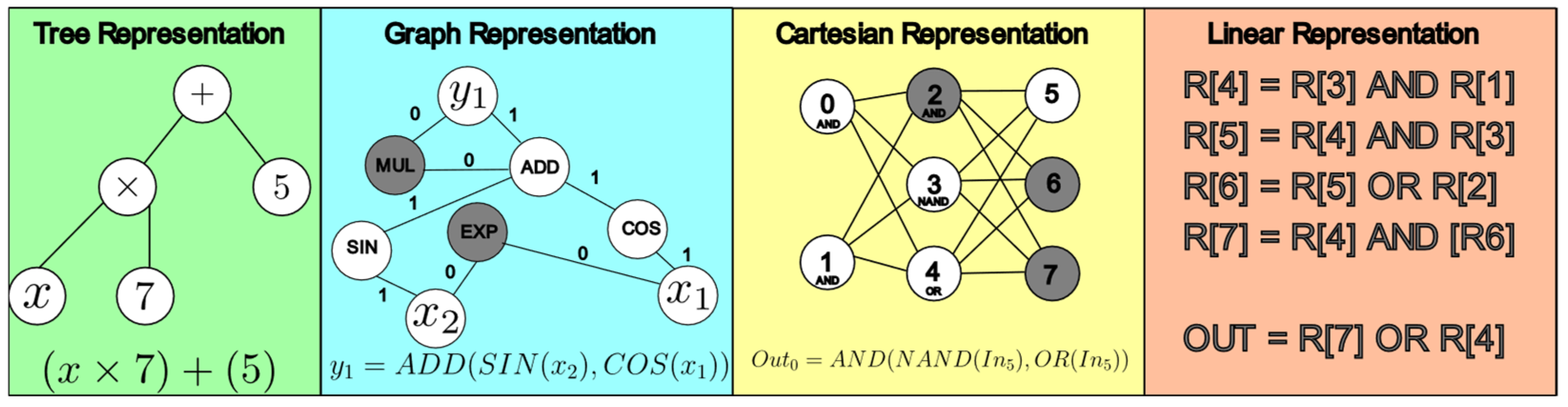
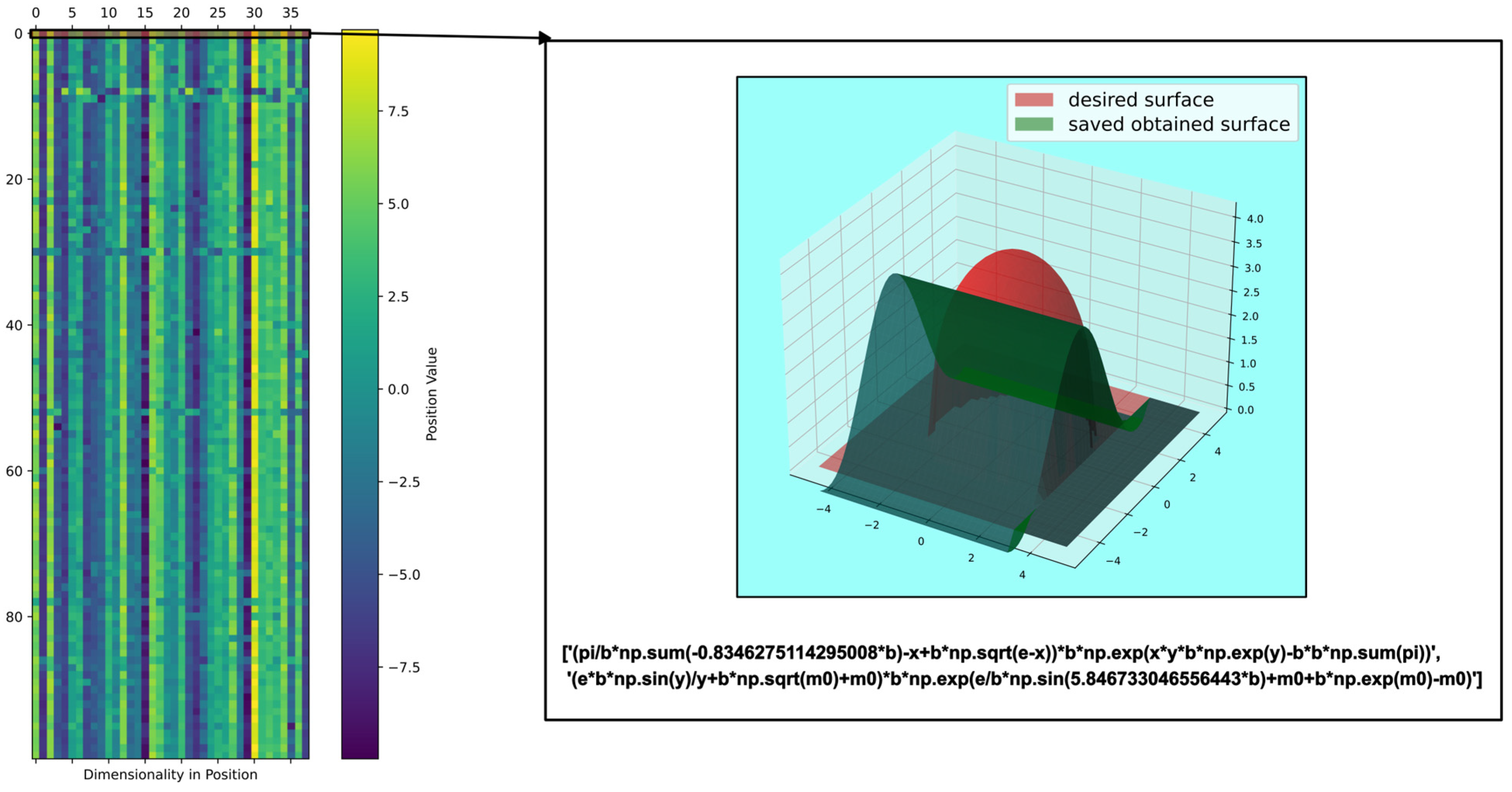
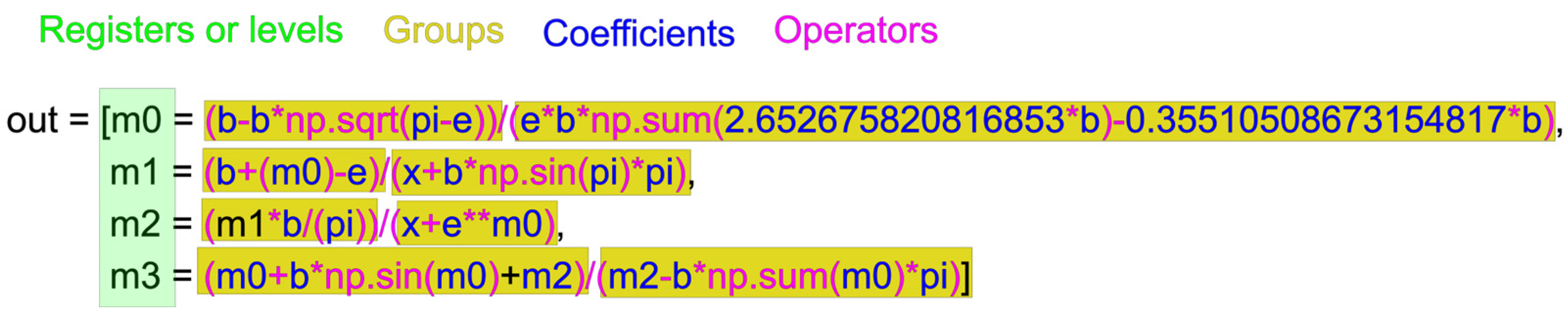
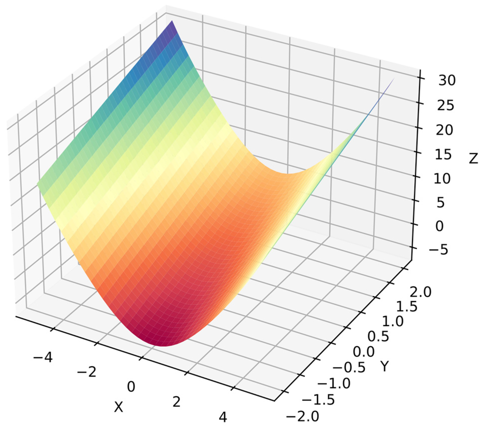


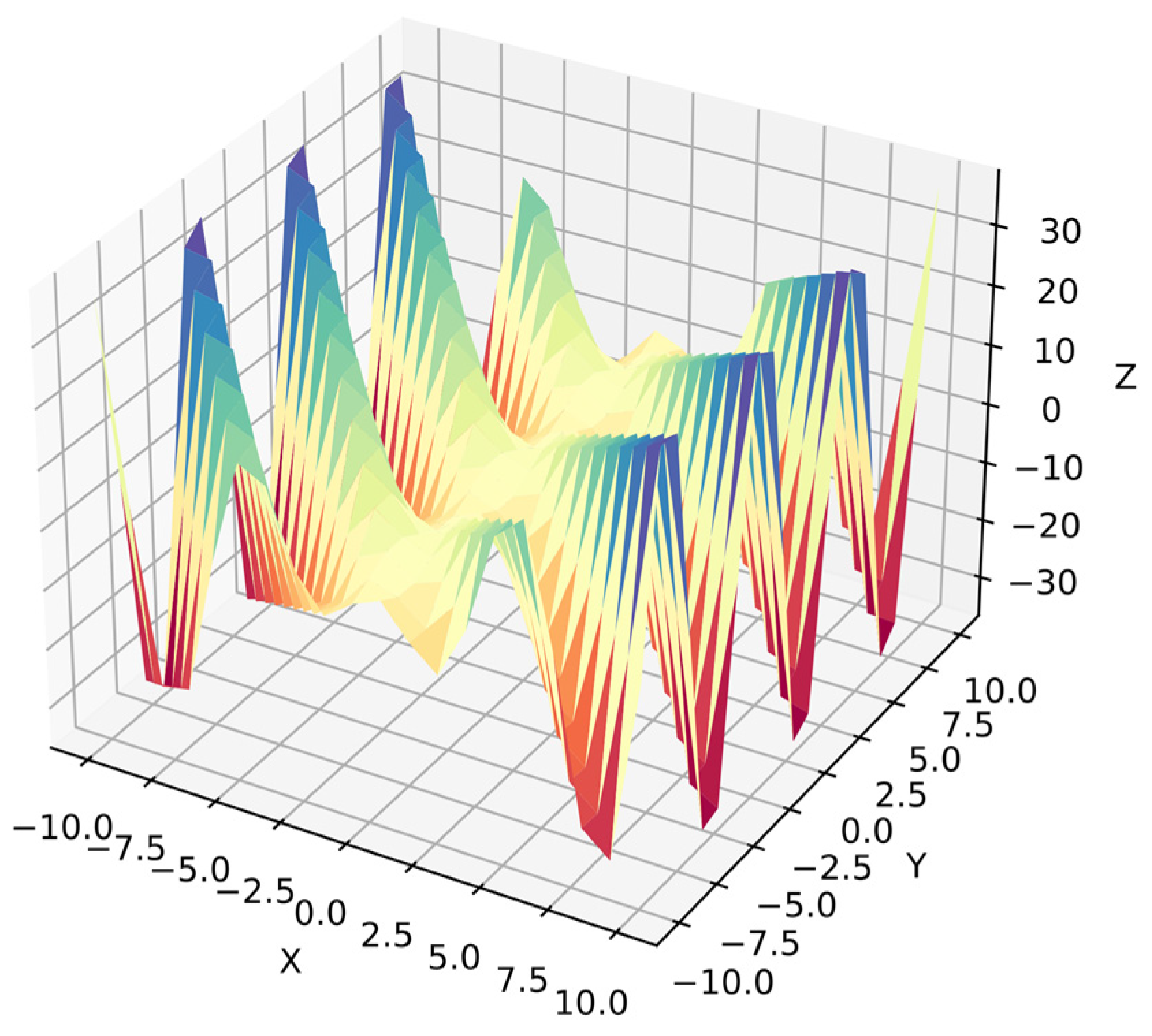


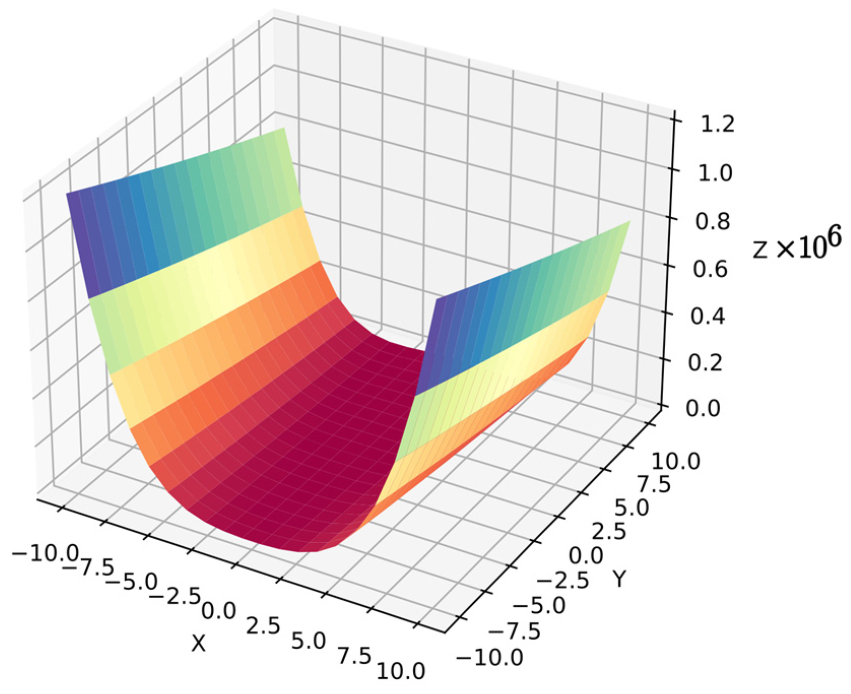

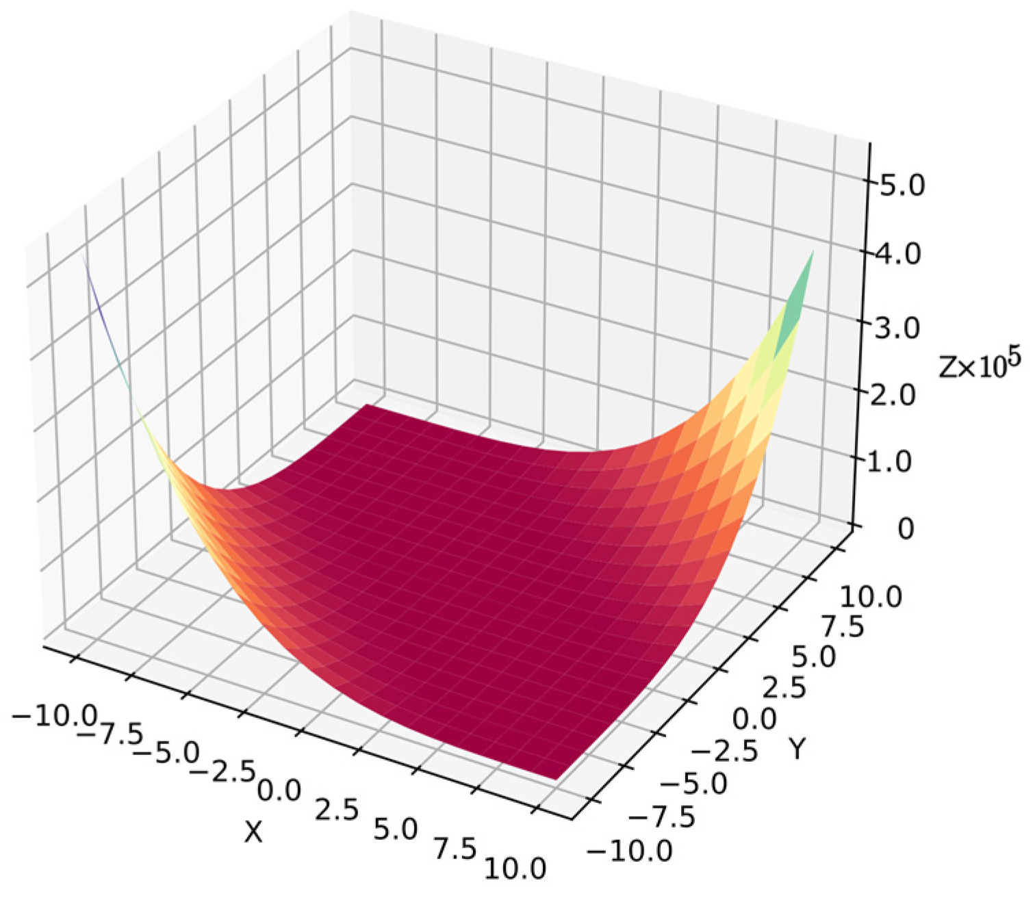
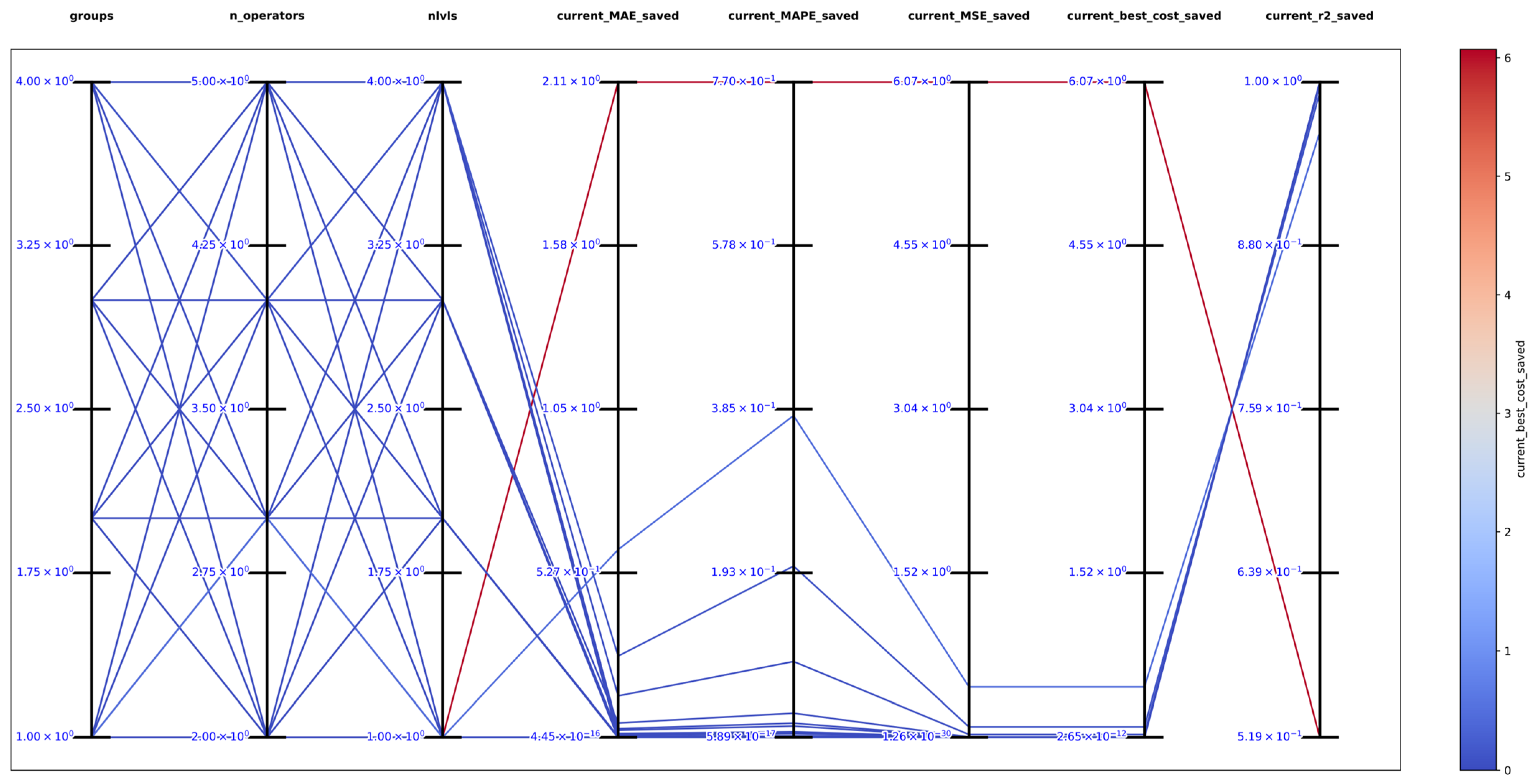

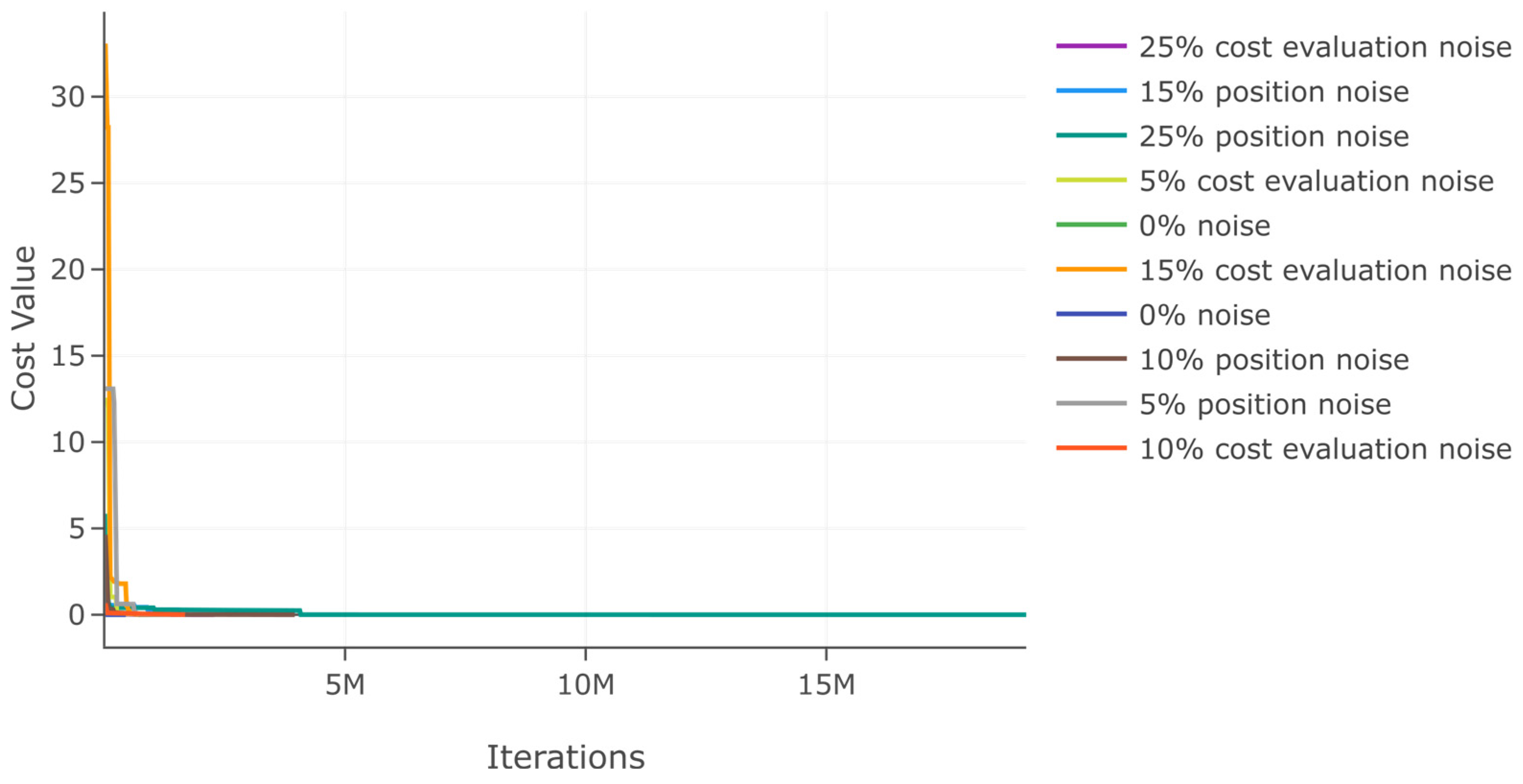
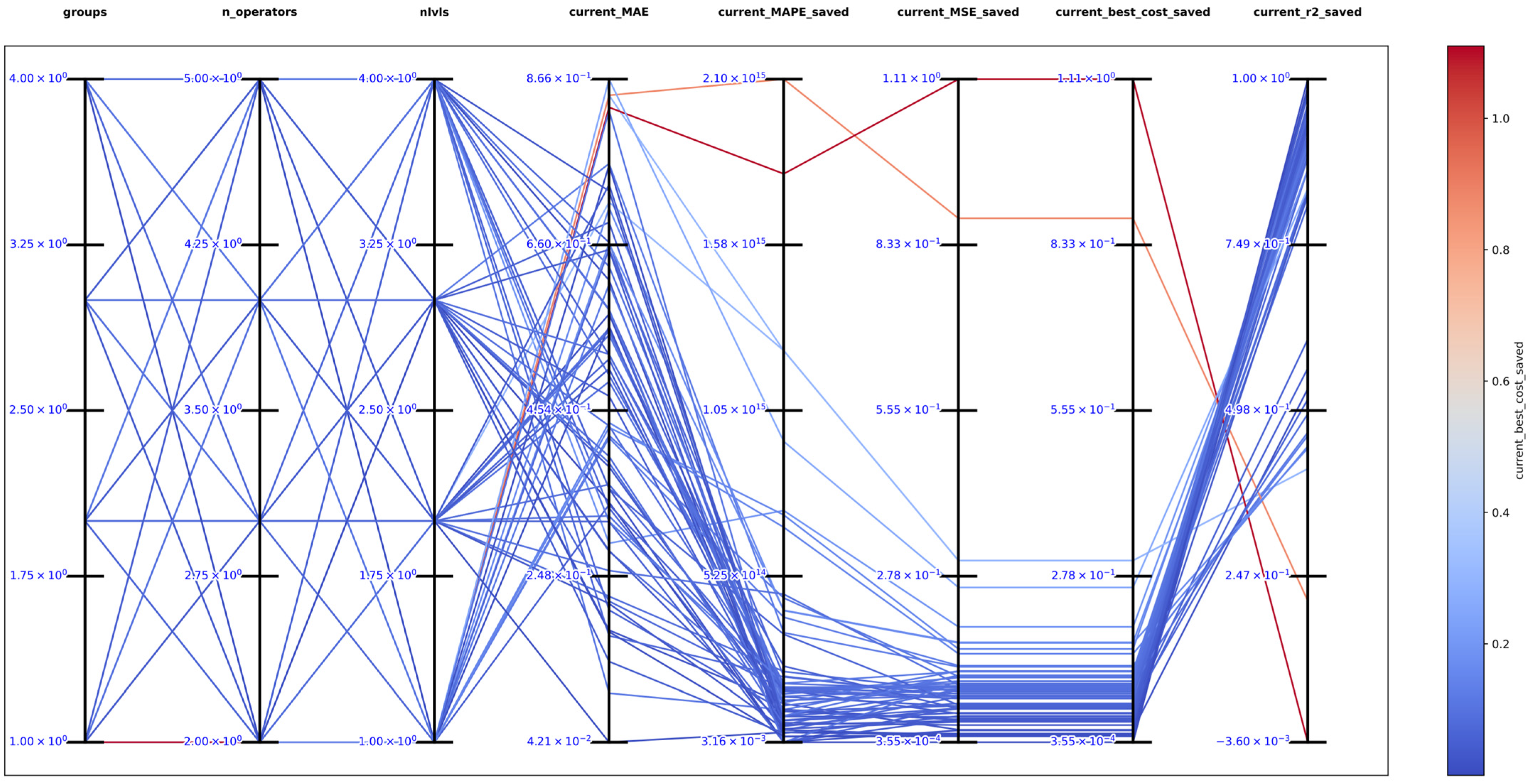
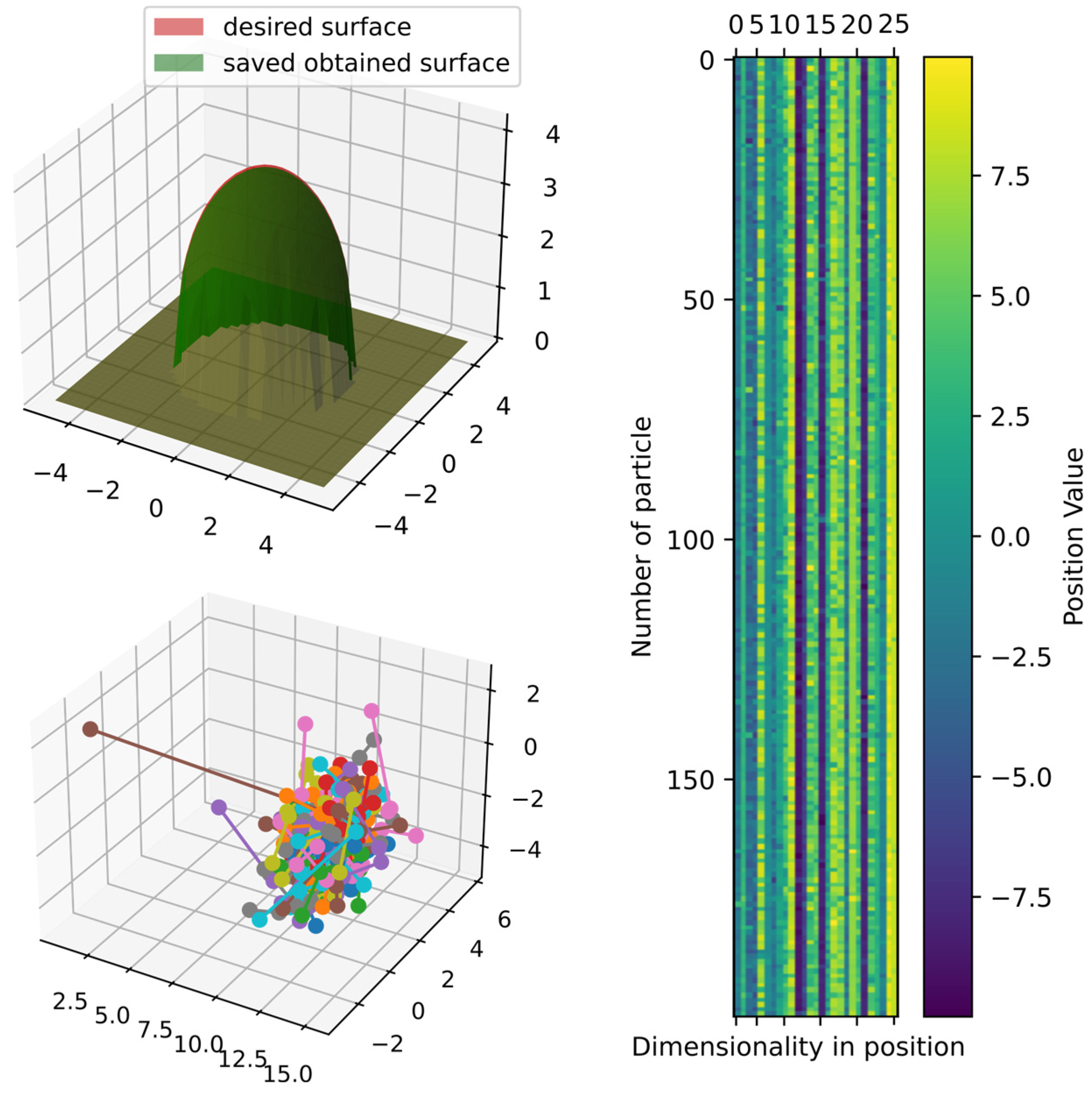
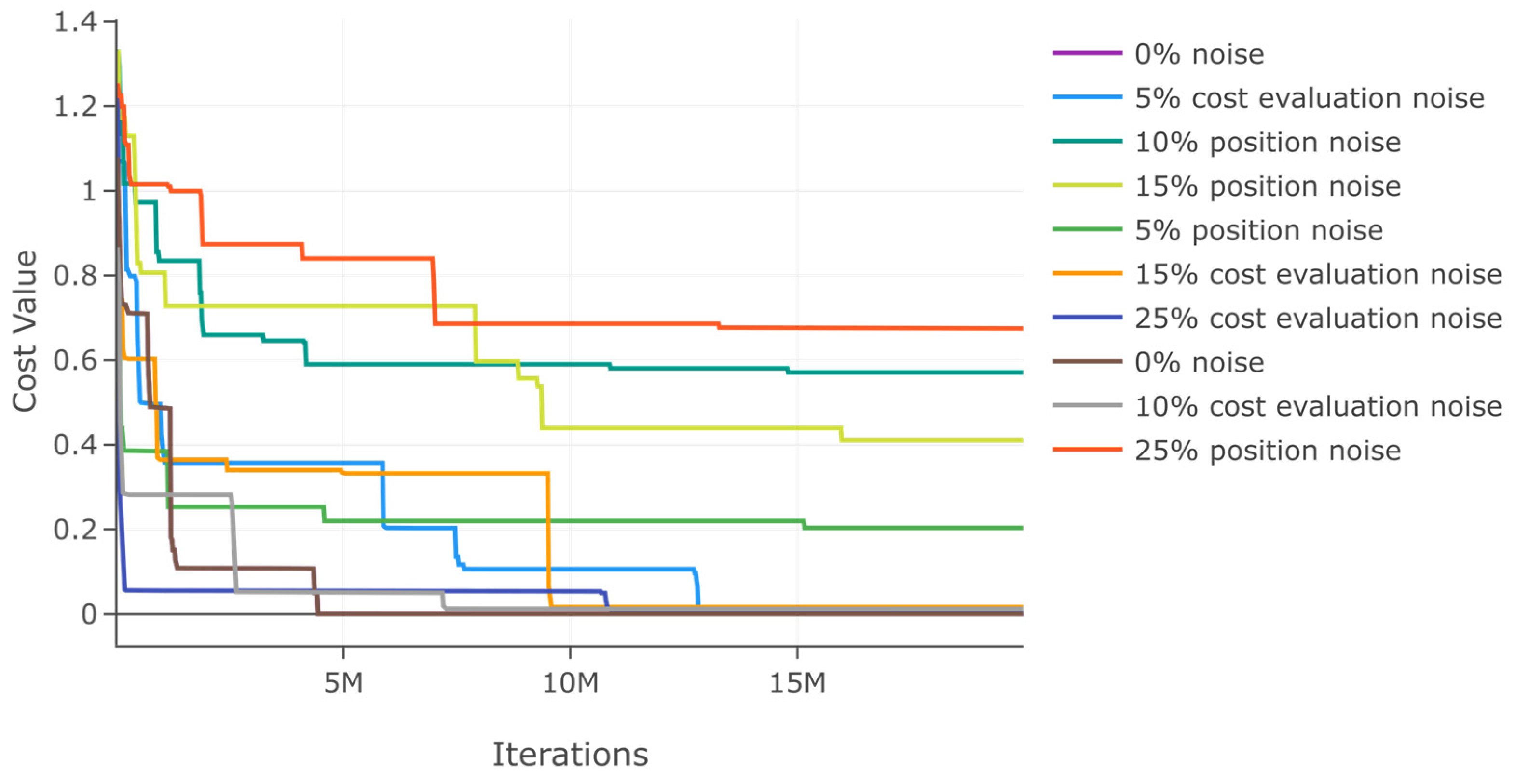
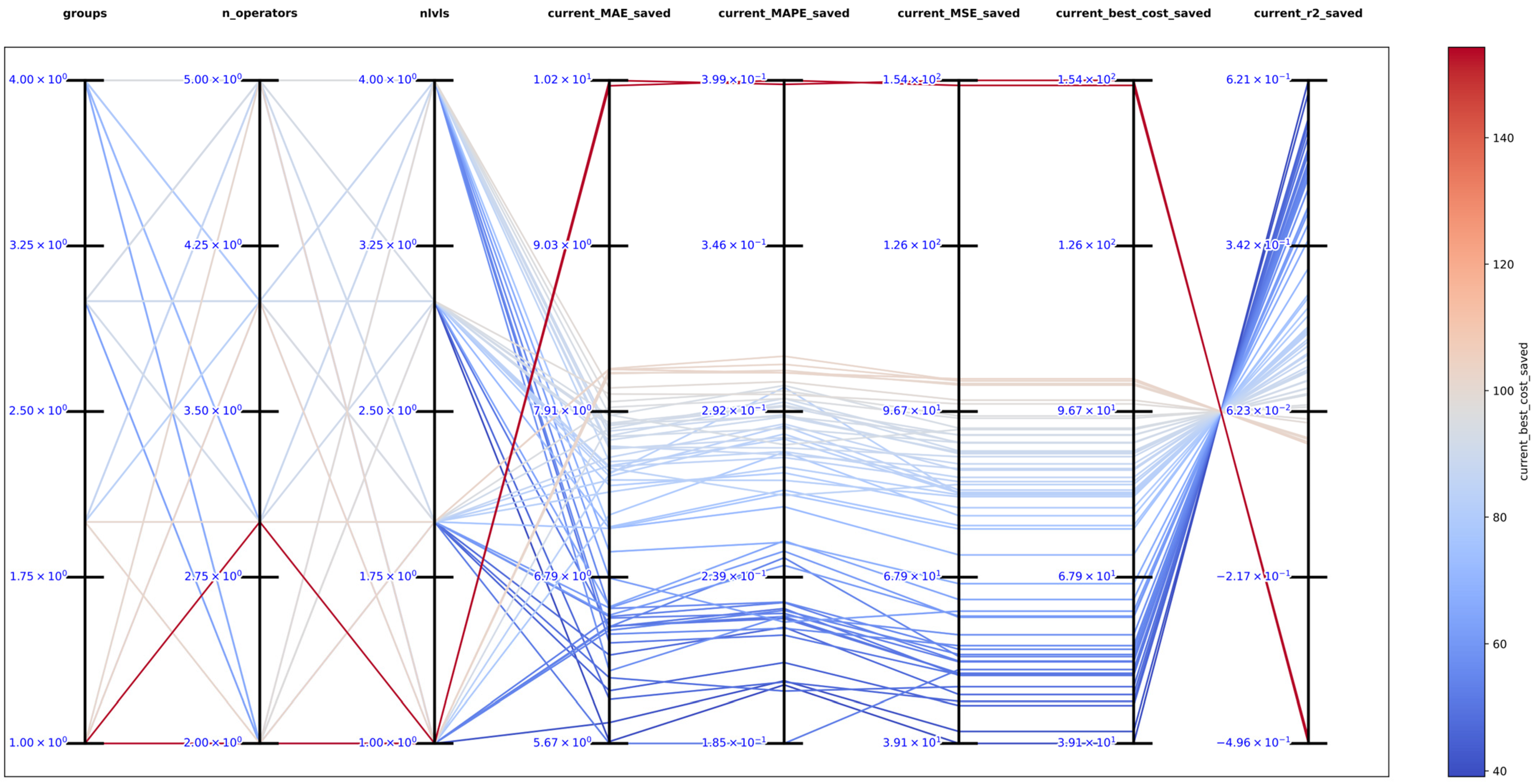
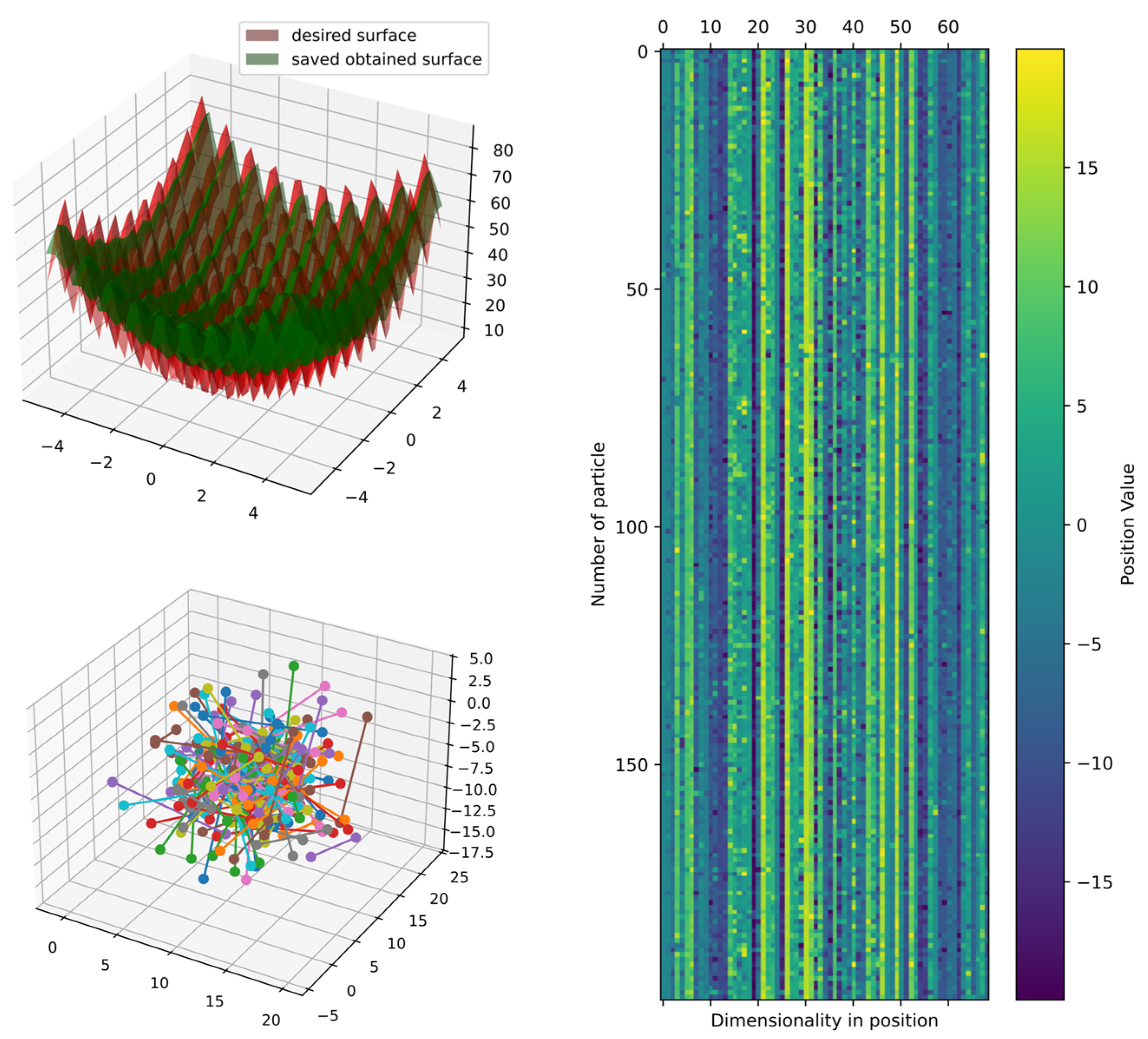
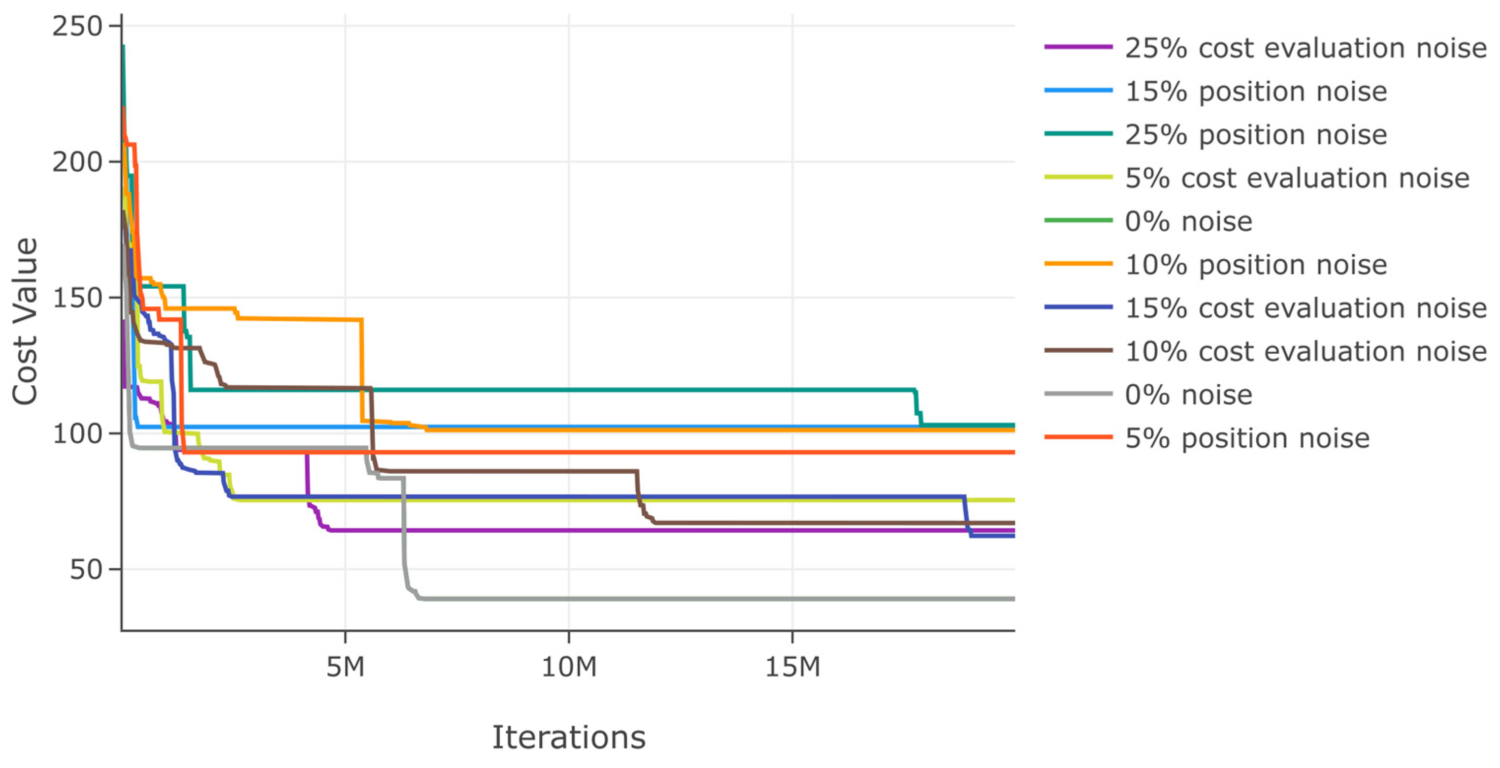
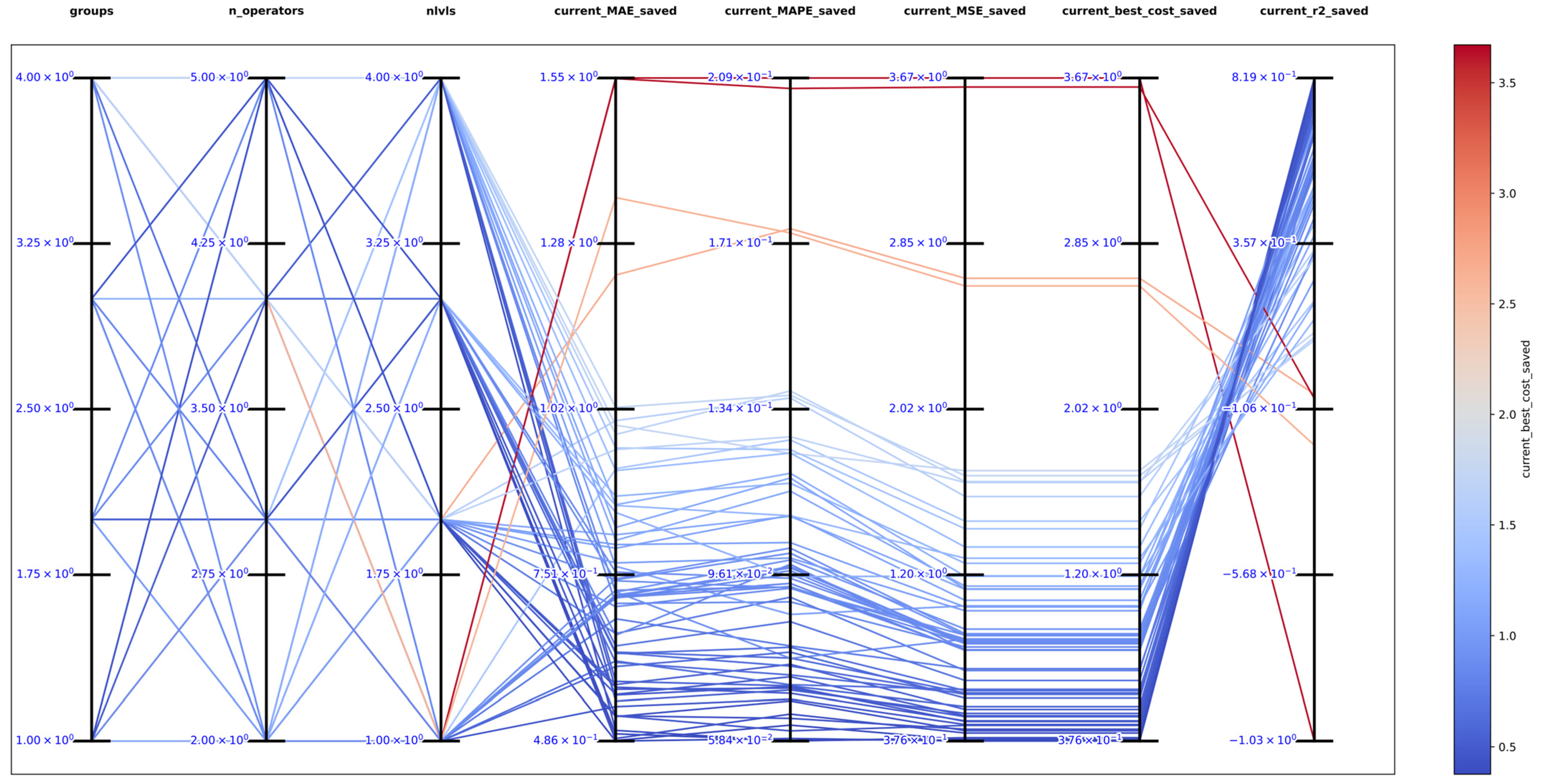
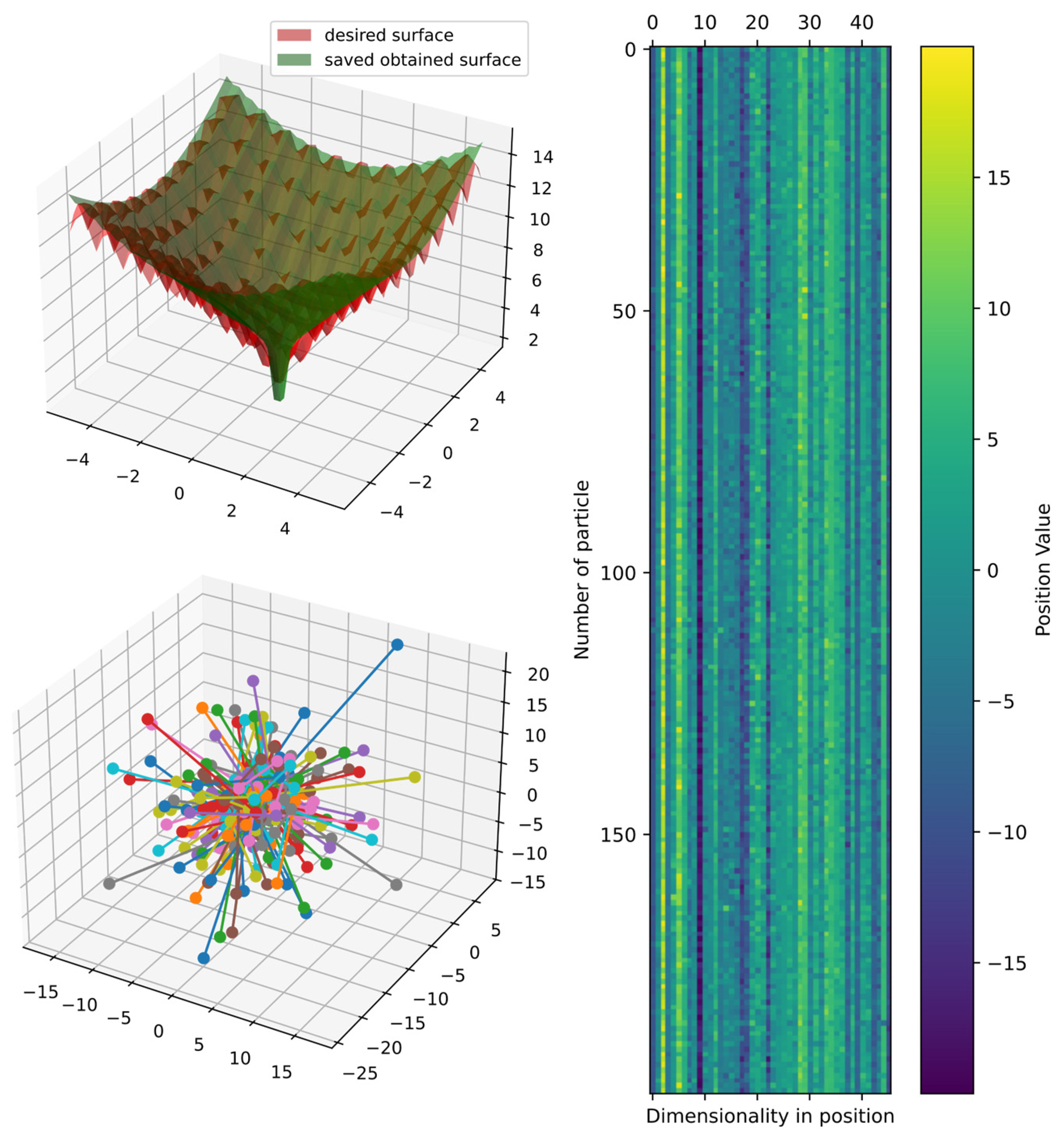
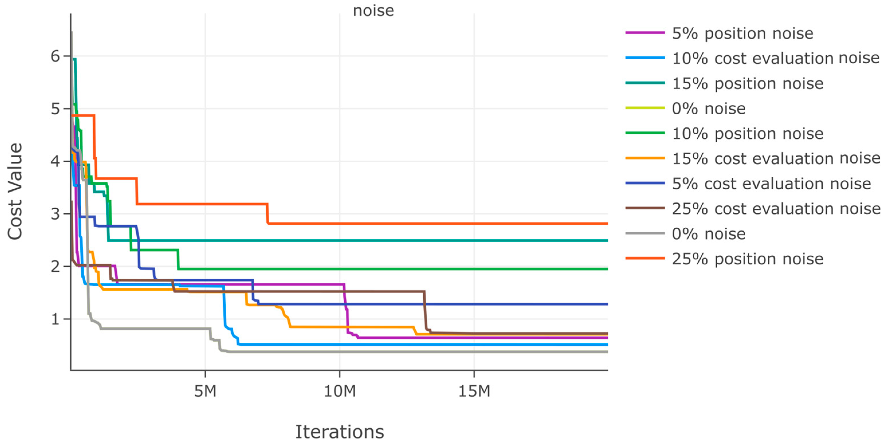
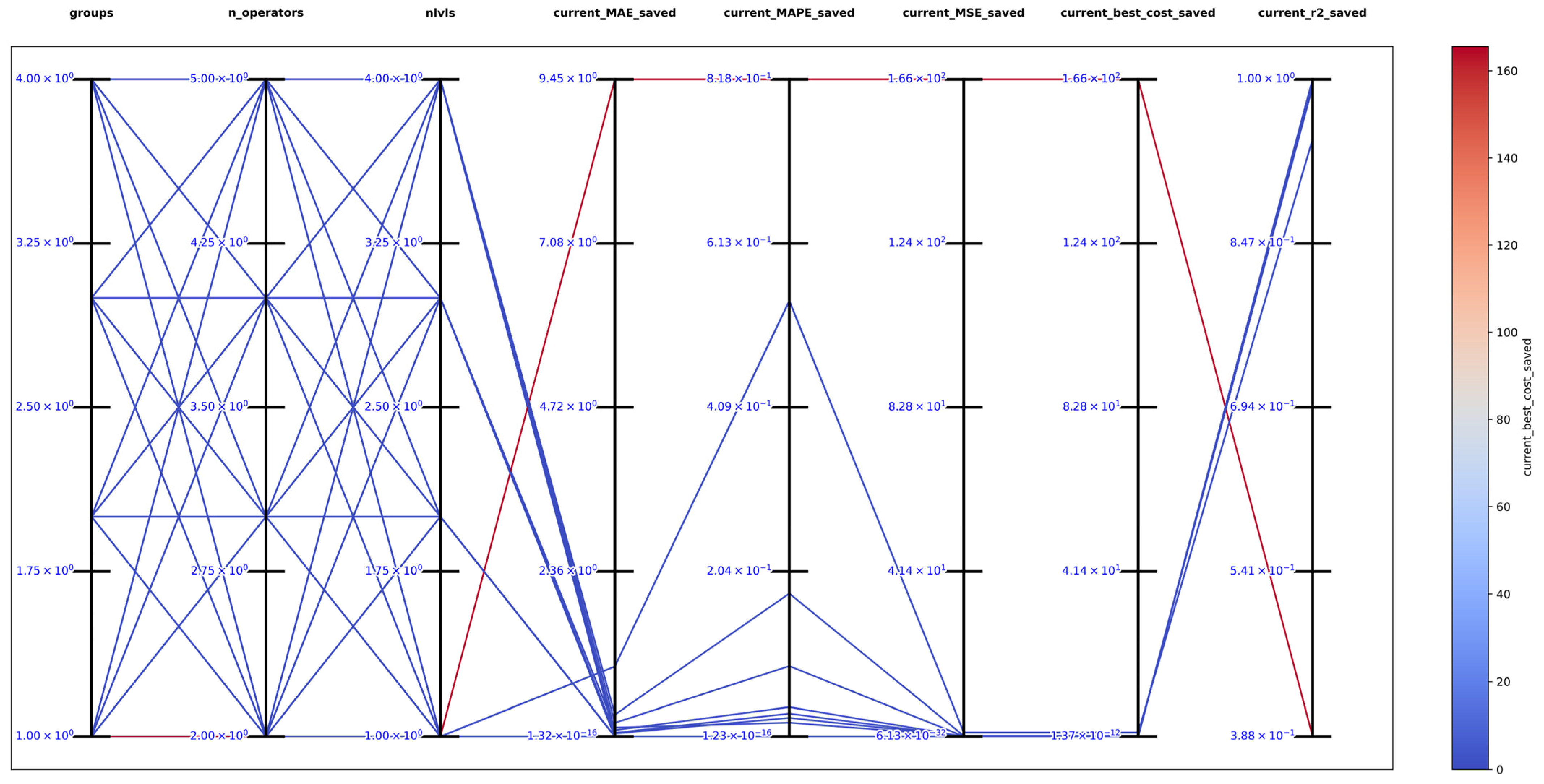

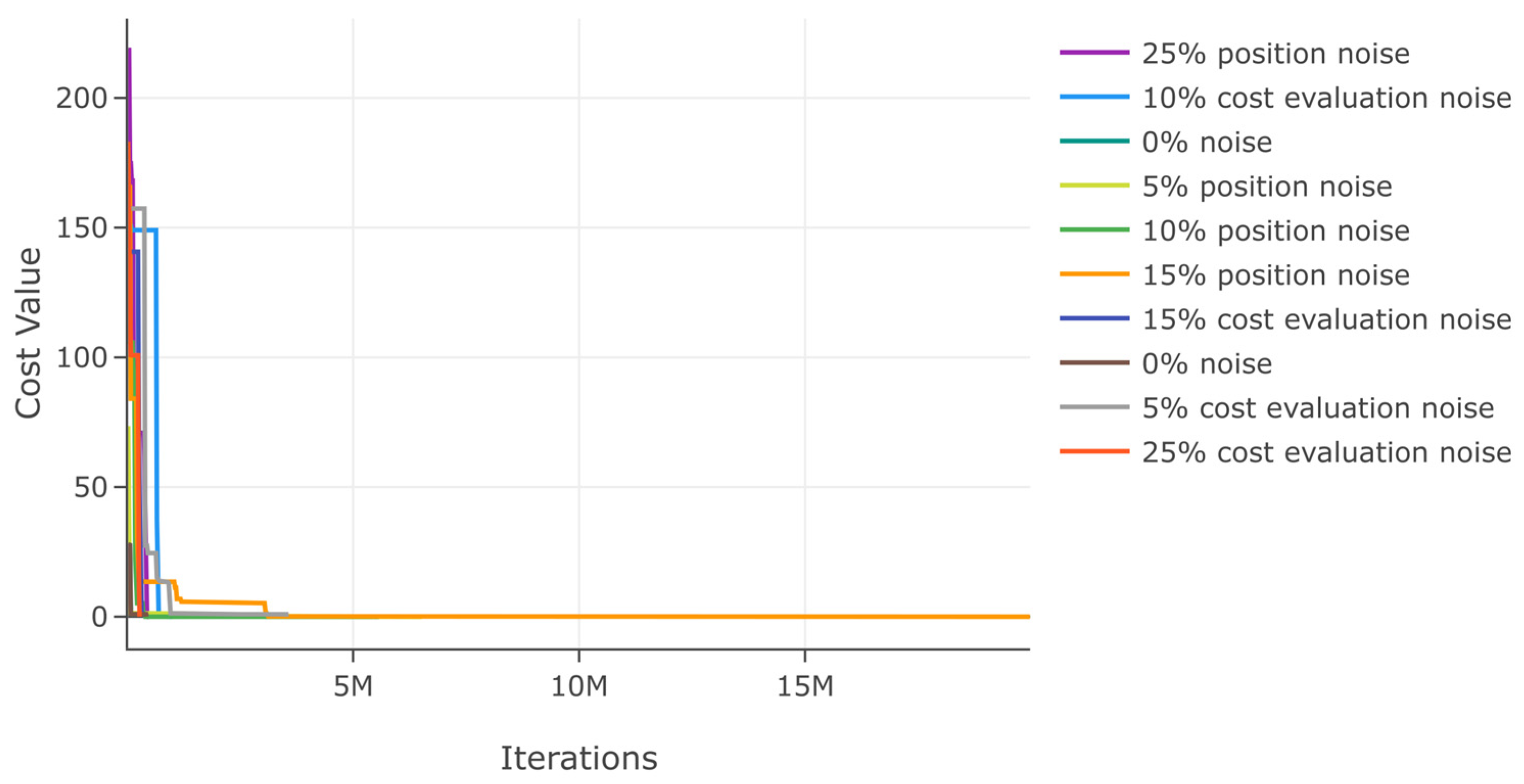
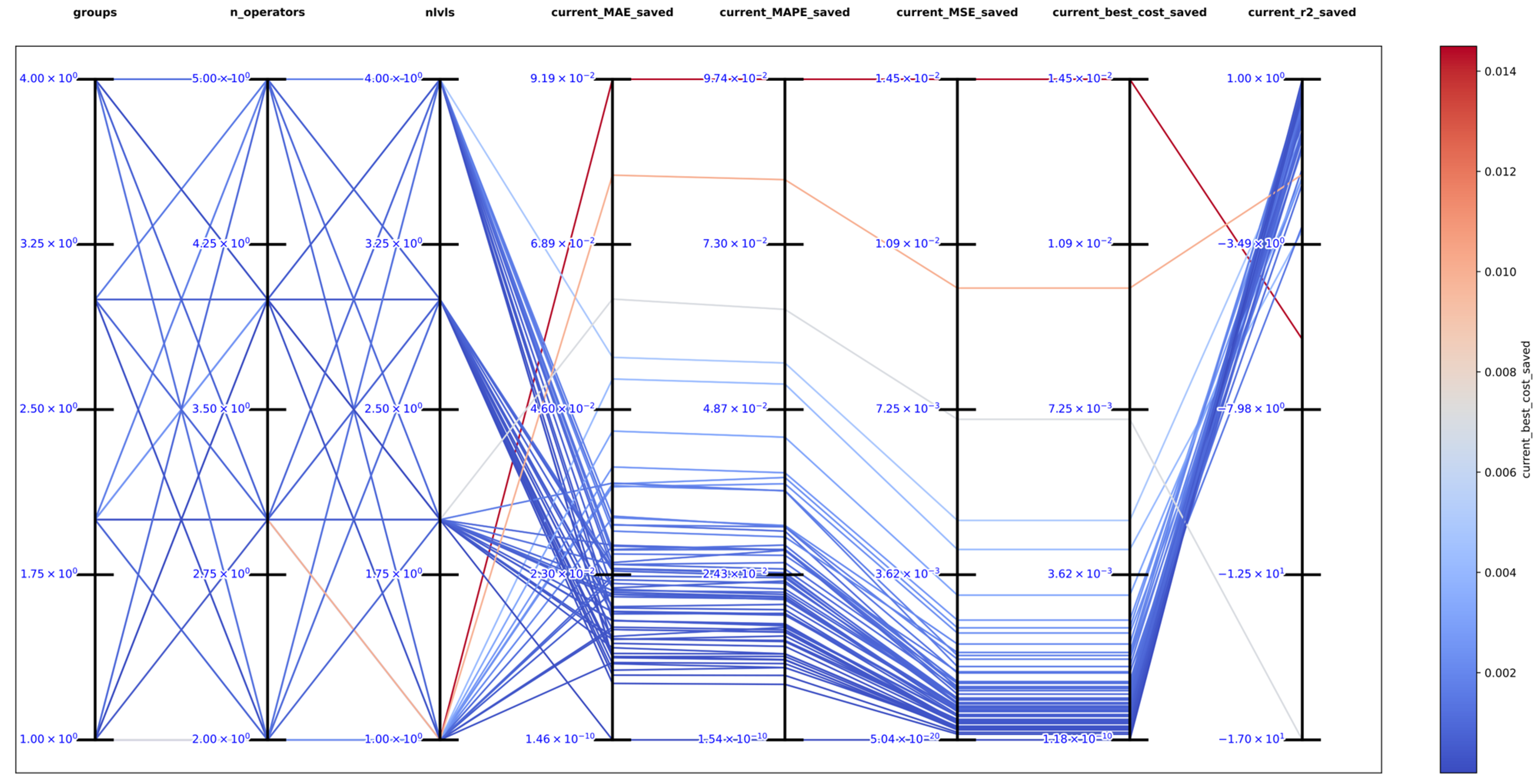
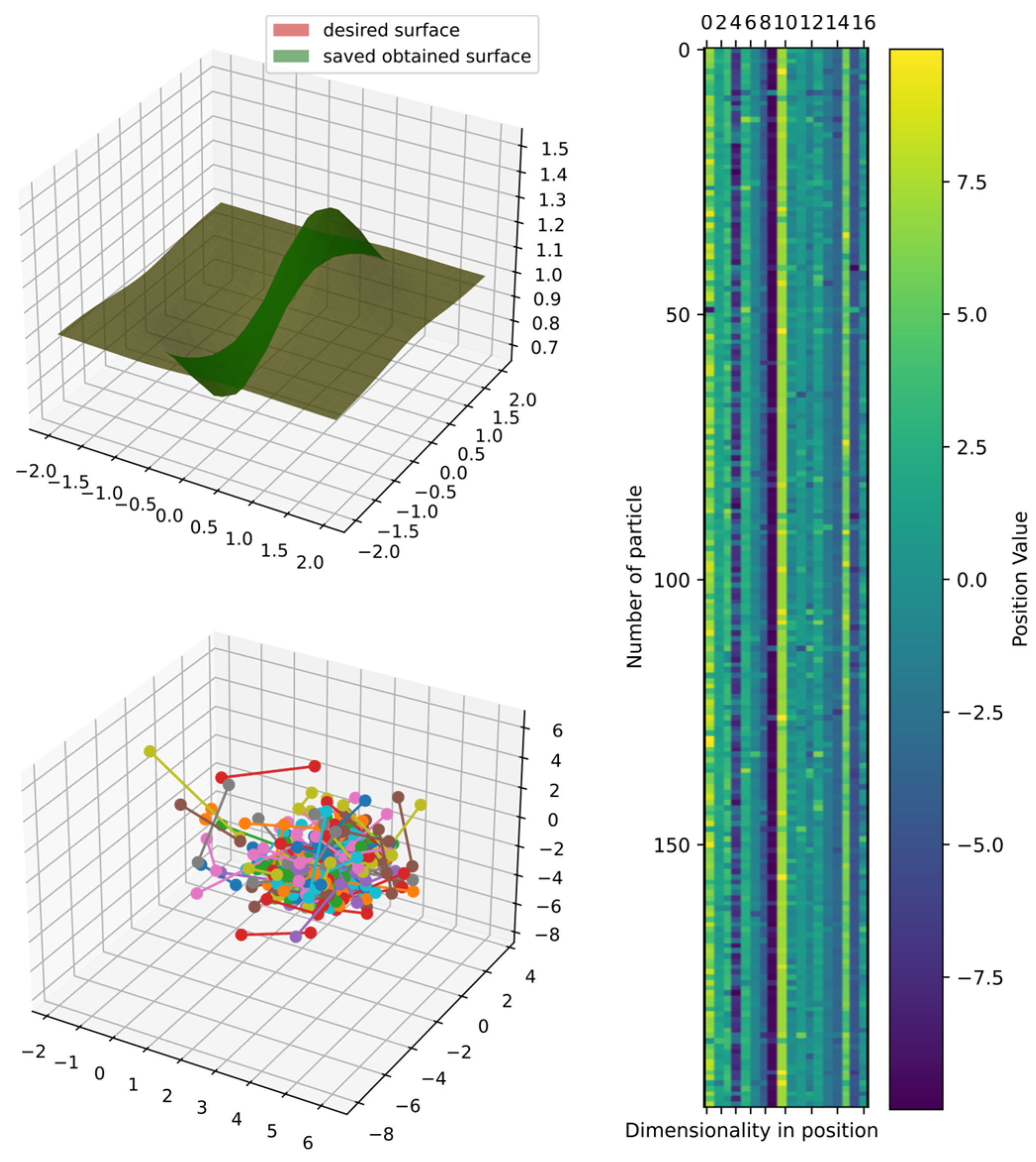
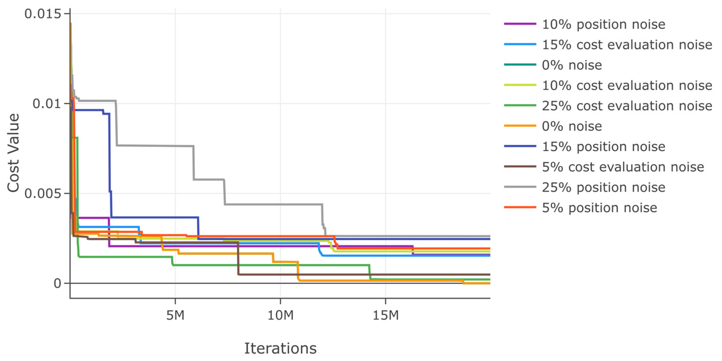
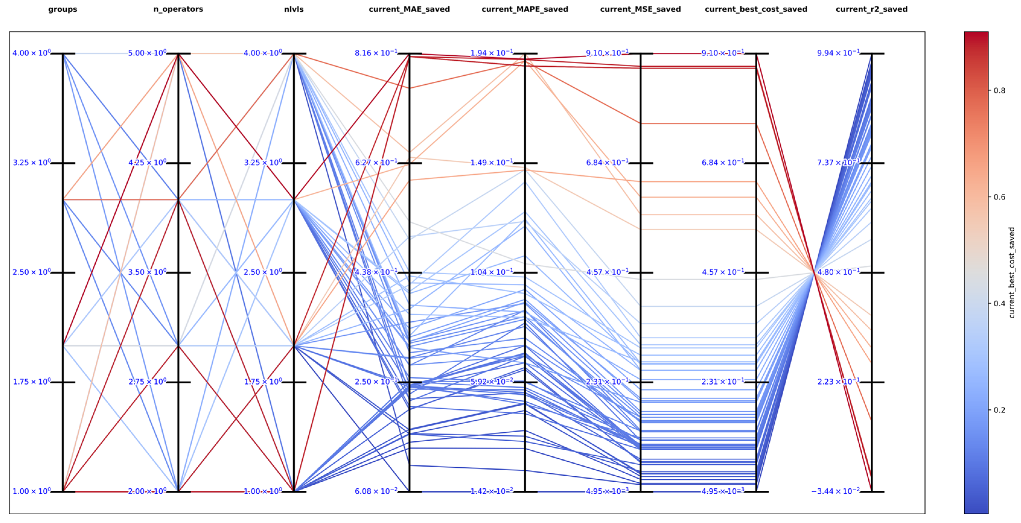
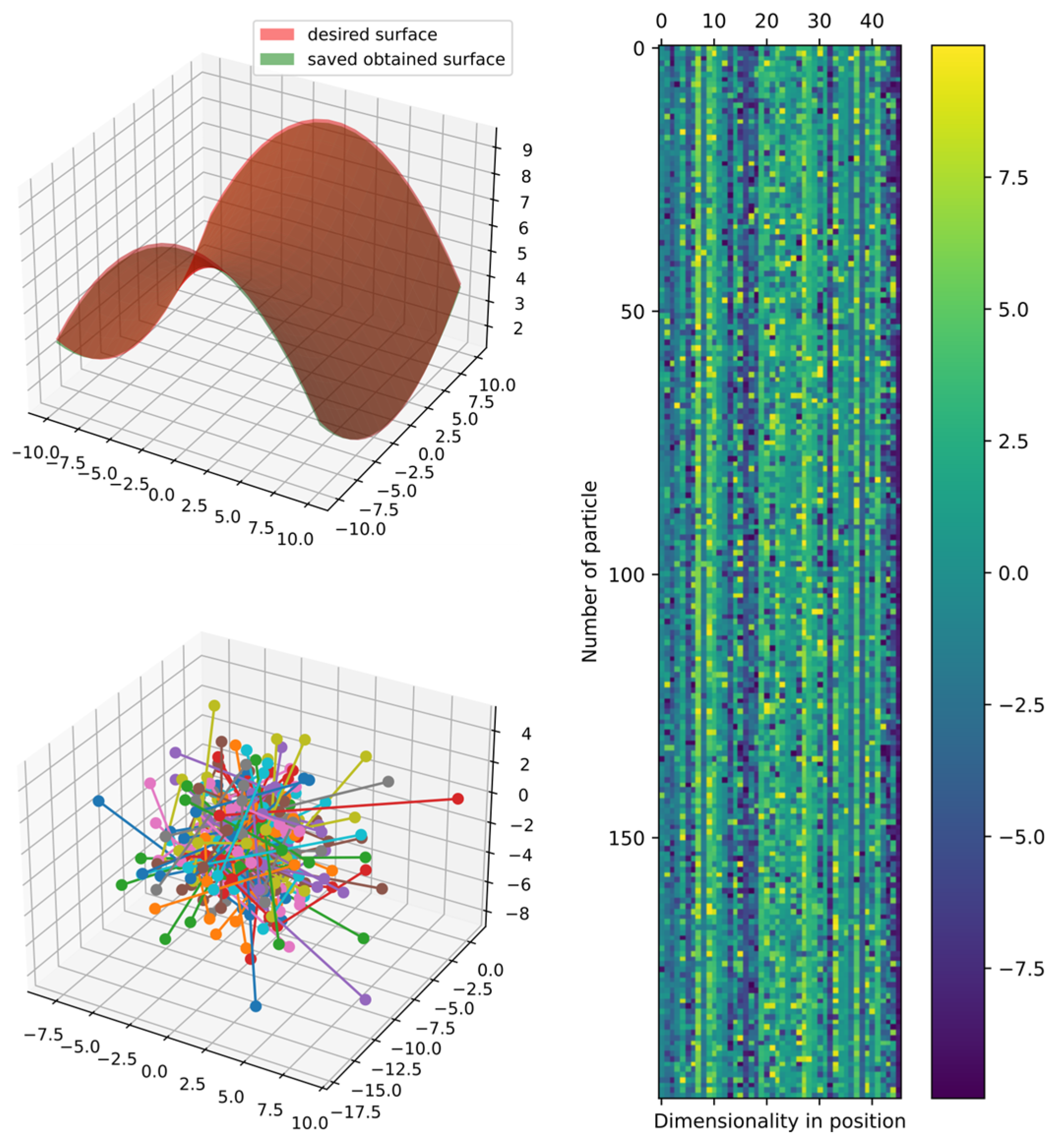
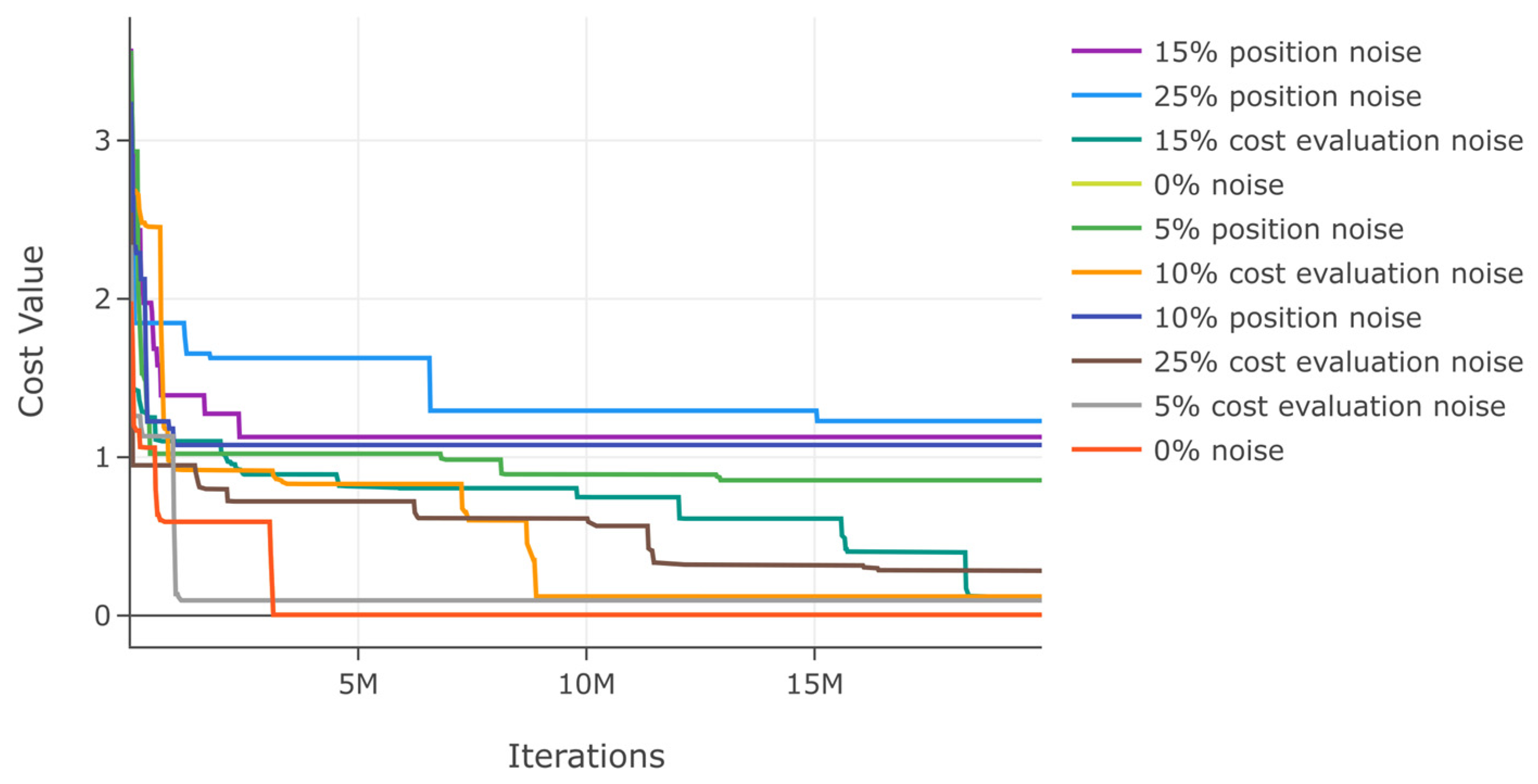
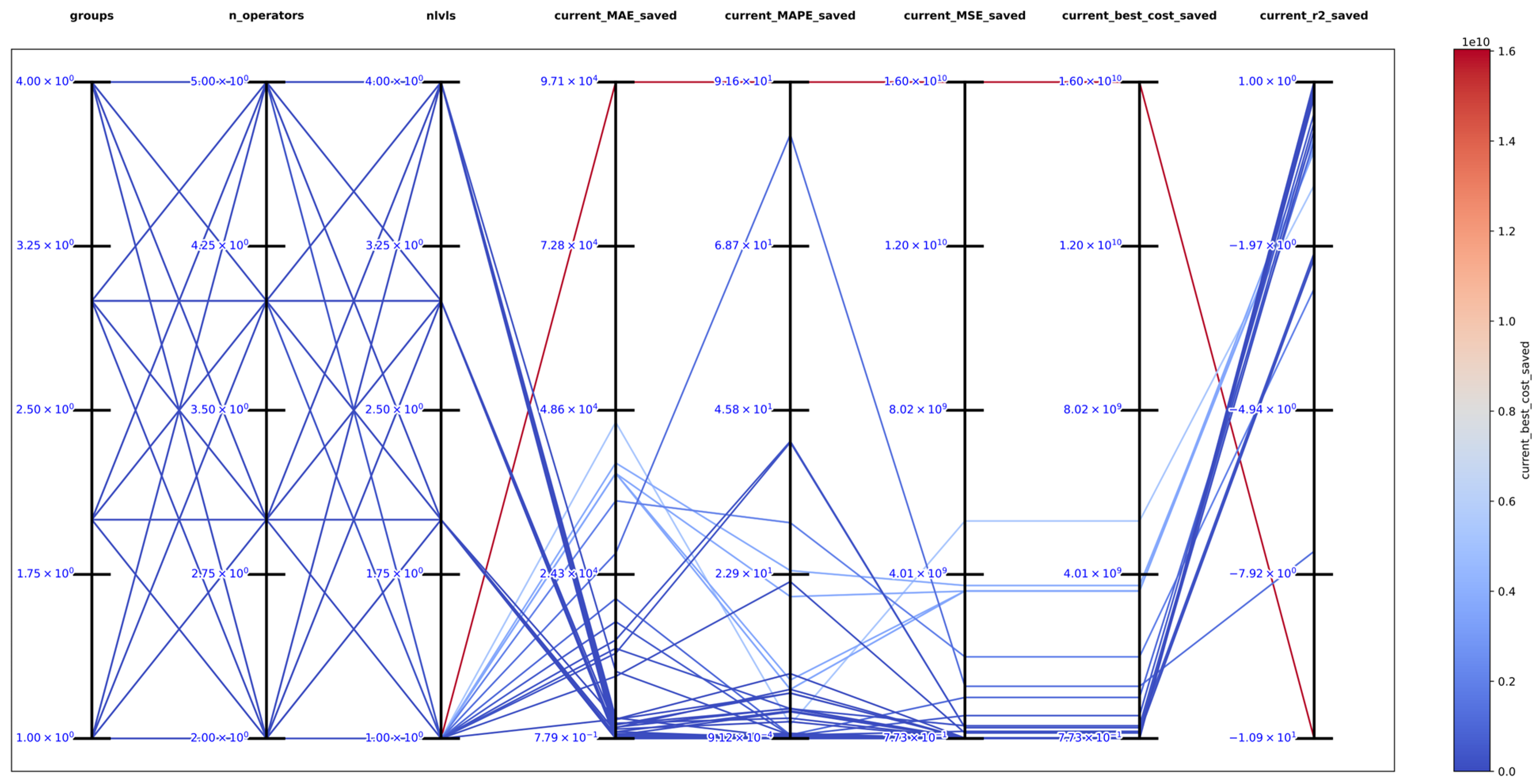
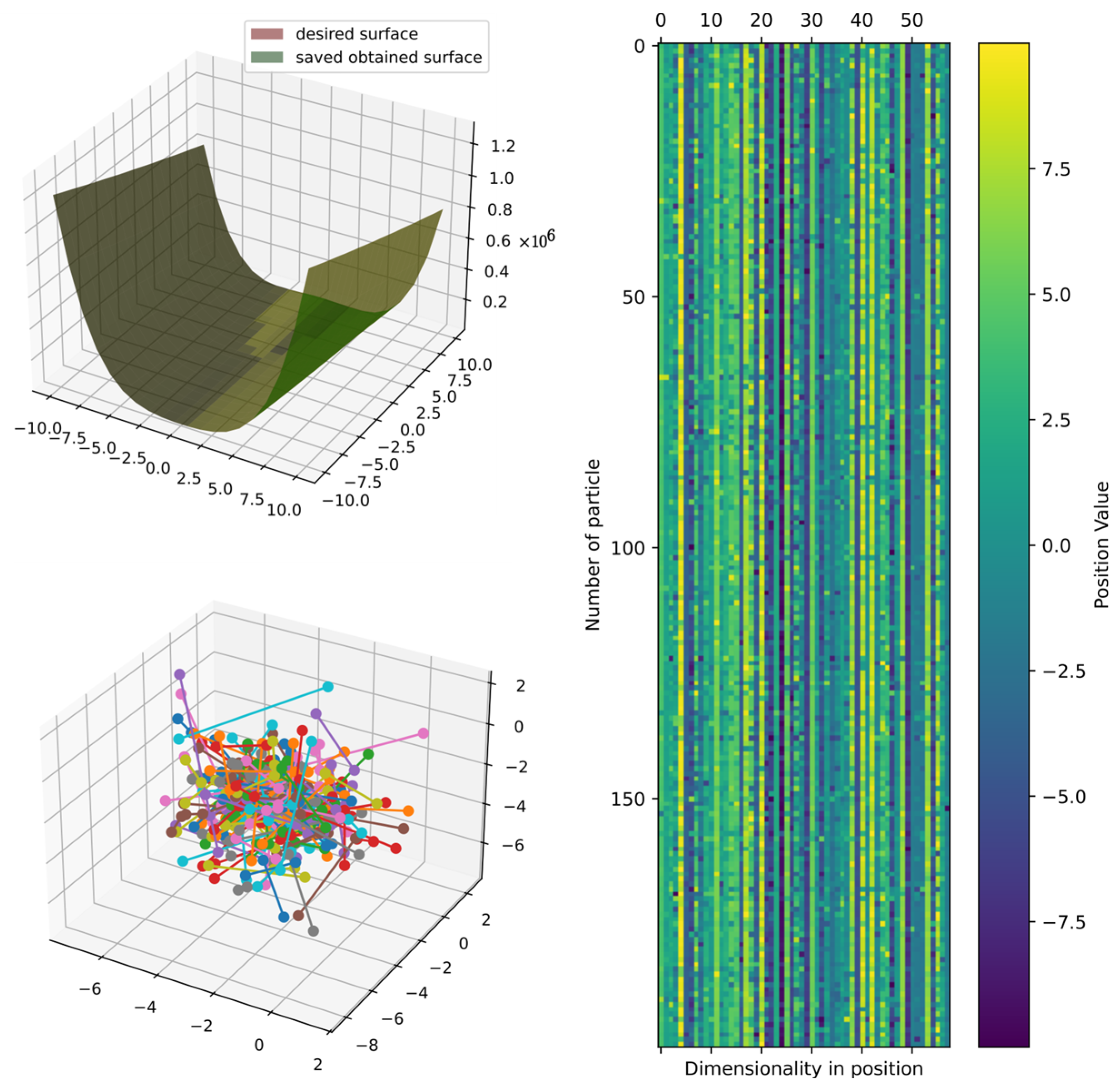
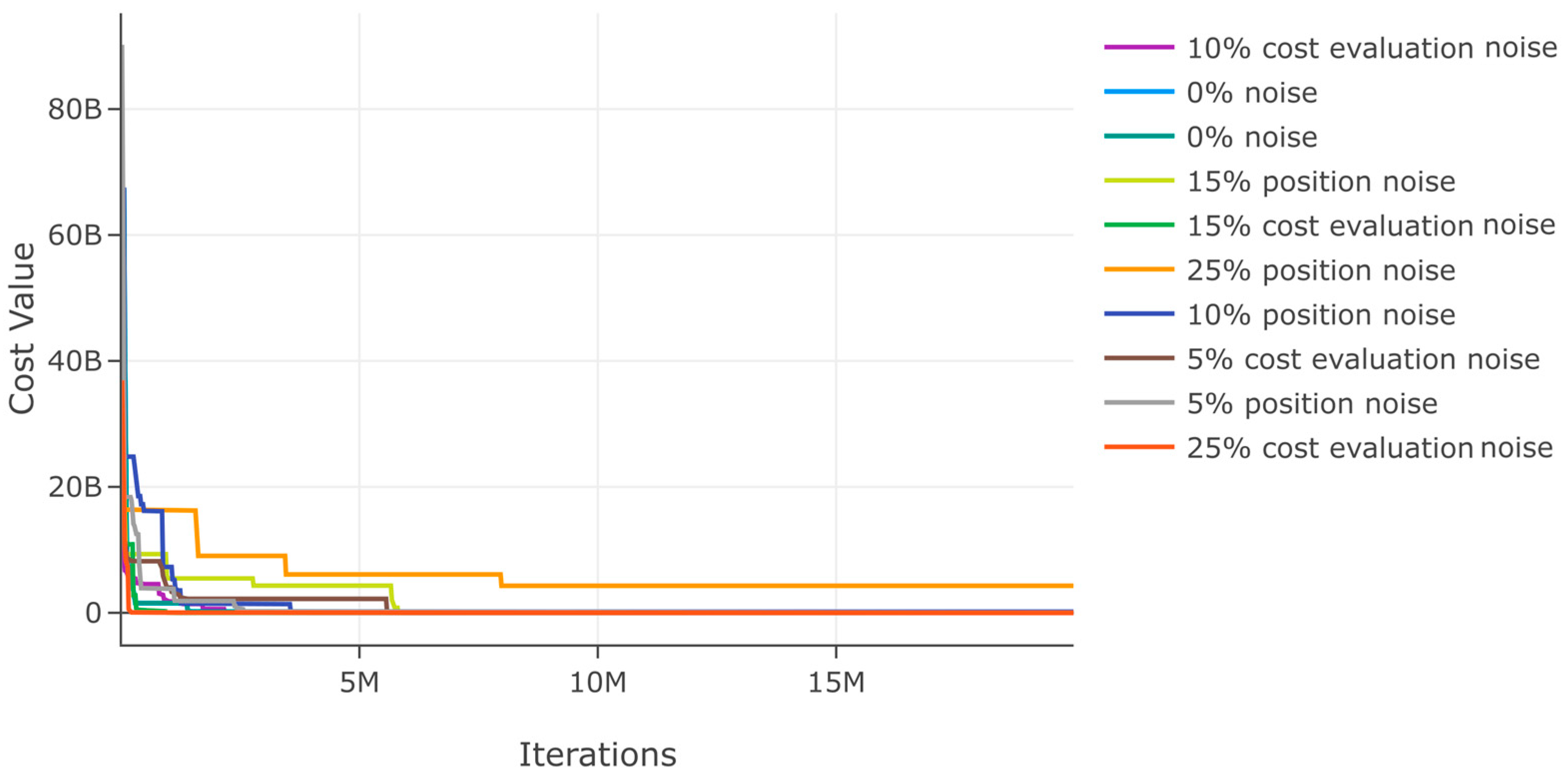


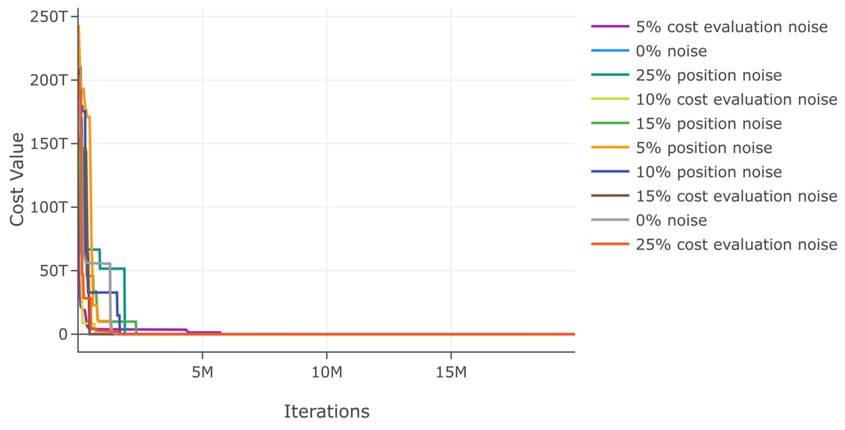
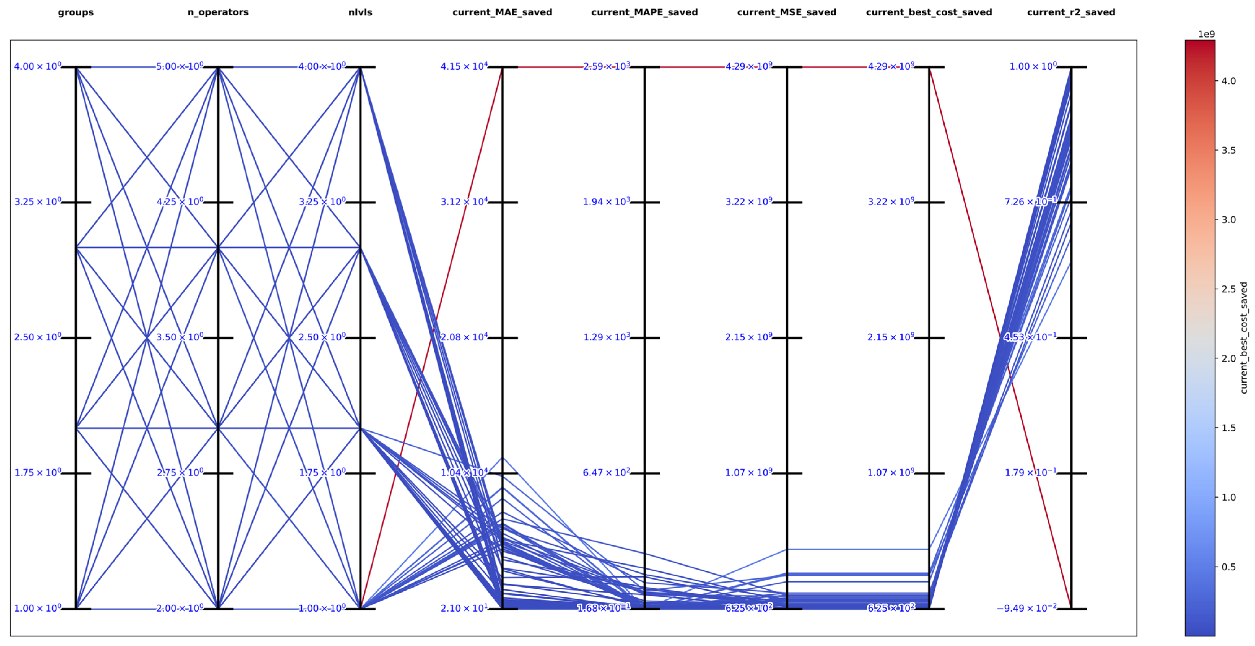
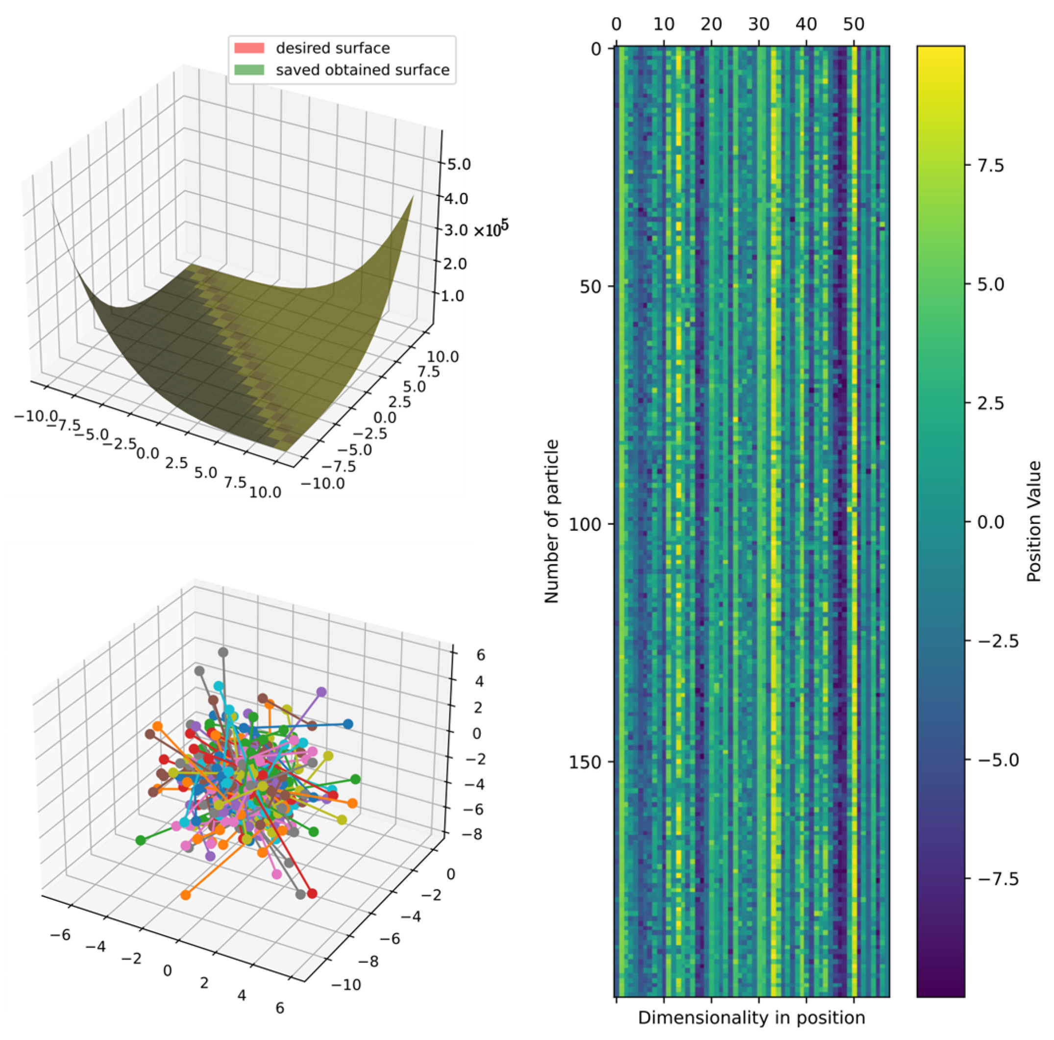
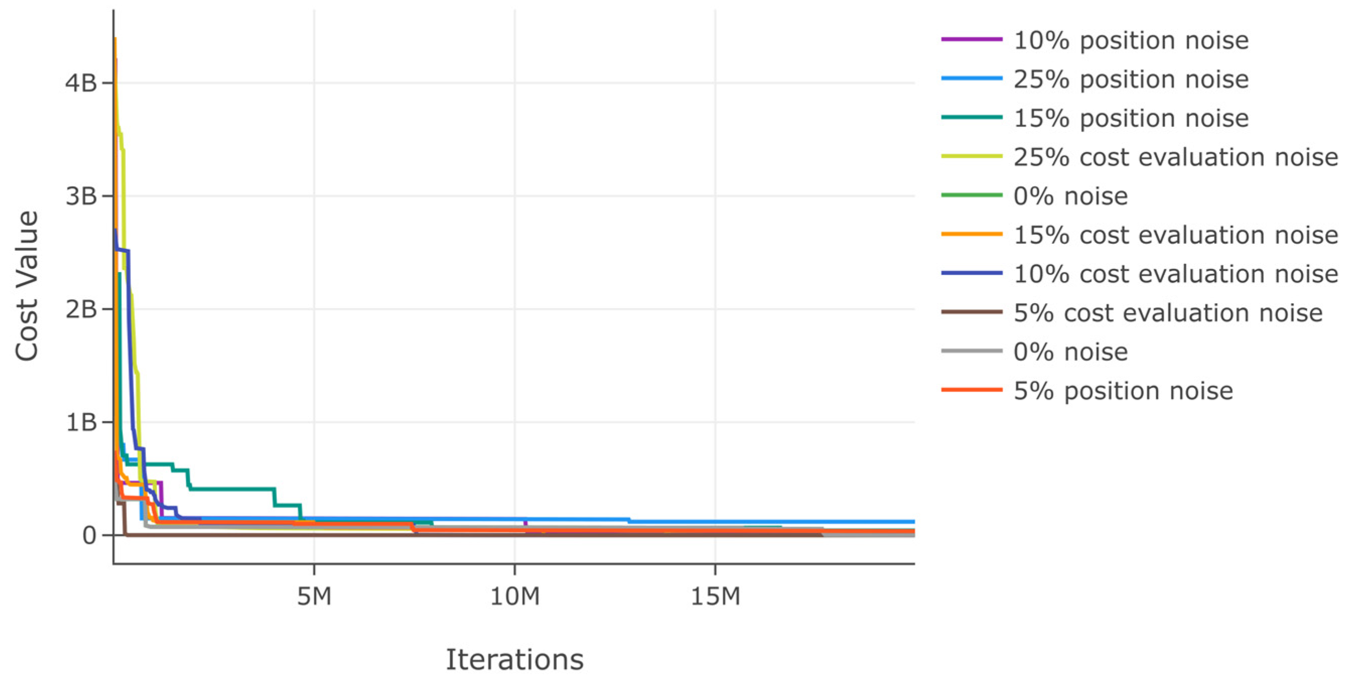
Disclaimer/Publisher’s Note: The statements, opinions and data contained in all publications are solely those of the individual author(s) and contributor(s) and not of MDPI and/or the editor(s). MDPI and/or the editor(s) disclaim responsibility for any injury to people or property resulting from any ideas, methods, instructions or products referred to in the content. |
© 2024 by the authors. Licensee MDPI, Basel, Switzerland. This article is an open access article distributed under the terms and conditions of the Creative Commons Attribution (CC BY) license (https://creativecommons.org/licenses/by/4.0/).