On the Univariate Vector-Valued Rational Interpolation and Recovery Problems

Abstract

In this paper, we consider a novel vector-valued rational interpolation algorithm and its application. Compared to the classic vector-valued rational interpolation algorithm, the proposed algorithm relaxes the constraint that the denominators of components of the interpolation function must be identical. Furthermore, this algorithm can be applied to construct the vector-valued interpolation function component-wise, with the help of the common divisors among the denominators of components. Through experimental comparisons with the classic vector-valued rational interpolation algorithm, it is found that the proposed algorithm exhibits low construction cost, low degree of the interpolation function, and high approximation accuracy.

1. Introduction

Vector-valued rational interpolation, as a classic topic in mathematics, has garnered significant attention due to its extensive applications in various fields, including mechanical vibration, data analysis, automatic control, and image processing, etc. [1,2,3,4,5]. In this paper, we primarily focus on the univariate vector-valued rational interpolation problem. The classical vector-valued rational interpolation can be stated as follows: Given a dataset

$$\{(x_i,{\overrightarrow{V}}_i):x_i\in \mathbb{R},{\overrightarrow{V}}_i=\overrightarrow{V}\left(x_i\right)=(V_1\left(x_i\right),V_2\left(x_i\right),\cdots ,V_s\left(x_i\right))=(v_{i,1},\dots ,v_{i,s})\in {\mathbb{R}}^s,i=1,2,\dots ,n\},$$

where each vector value ${\overrightarrow{V}}_i$ is associated with a distinct point $x_i$. We construct a vector-valued rational function

$$\overrightarrow{R}\left(x\right)={\displaystyle \frac{\overrightarrow{P}\left(x\right)}{Q\left(x\right)}},$$

such that

$$\overrightarrow{R}\left(x_i\right)={\displaystyle \frac{\overrightarrow{P}\left(x_i\right)}{Q\left(x_i\right)}}={\overrightarrow{V}}_i,i=1,2,\dots ,n,$$

where $\overrightarrow{P}\left(x\right)=(p_1\left(x\right),p_2\left(x\right),\cdots ,p_s\left(x\right))$ is an s-dimensional vector of polynomials, and $Q\left(x\right)$ is a real algebraic polynomial.

For a classical univariate vector-valued rational interpolation problem, Graves-Morris [6,7] proposed a Thiele-type algorithm based on the Samelson inverse transformation for vectors. They also proved the characteristic theorem and uniqueness of this kind of vector-valued rational interpolation. Subsequently, Graves-Morris and Jenkins [8] presented a Lagrange determinant algorithm for solving the classical vector-valued rational interpolation problems. Levrie and Bultheel [9] introduced a definition of generalized continued fractions and a Thiele n-fraction algorithm designed for the classical vector-valued rational interpolation. Zhu and Zhu [10] further contributed a recursive algorithm with inheritance properties for this type of interpolation.

Among various methods, the Thiele-type vector-valued rational interpolation algorithm [6] stands out as the most classic and widely used. It is discussed under the assumption of $Q\left(x\right)\mid {\left|\overrightarrow{P}\left(x\right)\right|}^2$. However, examples are found for which the rational interpolation functions constructed with this algorithm do not satisfy this assumption [11]. Therefore, this assumption actually limits the applicability of this algorithm and its uniqueness theorem. Furthermore, this algorithm may encounter a computation stall during the computation of inverted differences. In such cases, adjusting points or perturbing vector components becomes necessary for recalculation. This subsequently leads to an increase in computational complexity.

To make up for this deficiency, we propose a new vector-valued rational interpolation algorithm. Recognizing that vector-valued rational interpolation can be seen as a combination of multiple scalar rational interpolation problems, we construct a vector rational function in the form of

$$\overrightarrow{R}\left(x\right)=\left({\displaystyle \frac{p_1\left(x\right)}{q_1\left(x\right)}},{\displaystyle \frac{p_2\left(x\right)}{q_2\left(x\right)}},\cdots ,{\displaystyle \frac{p_s\left(x\right)}{q_s\left(x\right)}}\right)$$

(1)

to satisfy the interpolation conditions

$$\overrightarrow{R}\left(x_i\right)={\overrightarrow{V}}_i,i=1,2,\dots ,n,$$

where a non-trivial common divisor may exist between $q_i\left(x\right)$ and $q_j\left(x\right)$. This modification can expand the applicability of univariate vector-valued rational interpolation.

Based on the Fitzpatrick algorithm for univariate scalar rational interpolation, this paper develops a corresponding vector-valued version. It fully takes the advantage of common divisors among denominators. This algorithm can not only remove restrictions on the denominators of the interpolation function, but also avoid complicated calculations of inverse differences. When solving problems component-wise, we obtain denominators from the calculated components. These denominators are then used to reduce the degree of subsequent components. This inheritance gives the algorithm significant advantages in solving vector-valued rational function recovery problems and certain applications.

The paper is organized as follows: In Section 2, we provide a detailed introduction to the algorithm established for the univariate vector-valued rational interpolation function in the form of (1). In Section 3, we discuss how to handle vector-valued rational function recovery problem through introducing termination conditions. Finally, the application in solving positive-dimensional polynomial systems is considered.

2. Univariate Vector-Valued Rational Interpolation

In this section, we propose a univariate vector-valued rational interpolation algorithm based on the Fitzpatrick algorithm. The recursive property of the Fitzpatrick algorithm enables us to make full use of the common factors in the denominators of the already computed interpolation components, thereby reducing the degrees of the interpolation results for subsequent components. Before detailing our algorithm, we provide a brief overview of the Fitzpatrick algorithm; more details can be found in [12].

2.1. Fitzpatrick Algorithm for Univariate Scalar Rational Interpolation

Let  $\mathbb{K}$ be a field of characteristic 0. $\mathcal{P}=\mathbb{K}\left[x\right]$ is the univariate polynomial ring over  $\mathbb{K}$. Given a dataset

$$\{(x_i,v_i):x_i\in \mathbb{K},v_i\in \mathbb{K},i=1,2,\dots ,n\},$$

where each value $v_i$ is associated with a distinct point $x_i$. We construct a rational function

$$r\left(x\right)={\displaystyle \frac{a\left(x\right)}{b\left(x\right)}},$$

such that

$$r\left(x_i\right)={\displaystyle \frac{a\left(x_i\right)}{b\left(x_i\right)}}=v_i,i=1,2,\dots ,n,$$

where $a\left(x\right),b\left(x\right)\in \mathcal{P}$ and $b\left(x_i\right)\ne 0$, for $1\le i\le n$. The problem is referred to as the Cauchy-type rational interpolation problem [12].

This problem can be solved with the help of free modules and Gröbner basis methods. Let ${\mathcal{P}}^2$ be a free module with standard basis vectors ${\overrightarrow{e}}_1=(1,0)$ and ${\overrightarrow{e}}_2=(0,1)$. If $\overrightarrow{m}=x^{\alpha }{\overrightarrow{e}}_i$ for $i=1,2$, then $\overrightarrow{m}$ is called a monomial in ${\mathcal{P}}^2$.

Definition 1. 

For the order ${\prec }_{\xi }$ on ${\mathcal{P}}^2$, the following holds:

(1) $(x^i,0){\prec }_{\xi }(x^{i^{\prime }},0)$ if and only if $i<i^{\prime }$ and $(0,x^j){\prec }_{\xi }(0,x^{j^{\prime }})$ if and only if $j<j^{\prime }$;

(2) $(x^i,0){\prec }_{\xi }(0,x^j)$ if and only if $i\le j+\xi$;

where ξ is a given integer.

Fixing a monomial order ${\prec }_{\xi }$ in ${\mathcal{P}}^2$, each $(f,g)\in {\mathcal{P}}^2$ can be expressed as a $\mathbb{K}$-linear combination of monomials:

$$(f,g)=\sum _{i=1}^t{c}_i{\overrightarrow{m}}_i,$$

where $c_i\in \mathbb{K}$, $c_i\ne 0$, and ${\overrightarrow{m}}_1{\succ }_{\xi }{\overrightarrow{m}}_2{\succ }_{\xi }\cdots {\succ }_{\xi }{\overrightarrow{m}}_t$. The leading term of $(f,g)$ is defined as $LT(f,g)=c_1{\overrightarrow{m}}_1$. Additionally, the degree of the rational function $f/g$ is defined as $m_{\xi }(f,g)=max\{\delta f,\delta g+\xi \}$, where $\delta$ denotes the degree of the polynomial.

Let $I_i=⟨x-x_i⟩,i=1,2,\cdots ,n$, be the ideals in $\mathcal{P}$. If there exist  $a\left(x\right),b\left(x\right)\in \mathbb{K}\left[x\right]$ such that

$$a\left(x\right)-b\left(x\right)v_i\equiv 0mod{I}_i,i=1,\dots ,n,$$

then the pair $(a\left(x\right),b\left(x\right))\in {\mathcal{P}}^2$ is called a weak interpolation for the univariate Cauchy-type rational interpolation problem. It is easy to verify that for each positive integer k, the subset

$$M_k=\left\{(a\left(x\right),b\left(x\right))\right|a\left(x\right)-b\left(x\right)v_i\equiv 0mod{I}_i,i=1,\dots ,k\}$$

is a $\mathcal{P}$-submodule. Let $M_0={\mathcal{P}}^2$. Then, we have $M_0\supset M_1\supset \cdots \supset M_n=M$. If a fixed monomial order ${\prec }_{\xi }$ in ${\mathcal{P}}^2$ is given, and it is known that the Gröbner basis of $M_0$ is $\left\{\right(1,0),(0,1\left)\right\}$, then the Gröbner basis of $M_k$ for $k=1,2,\dots ,n$ can be recursively computed from that of $M_0$ with the Fitzpatrick algorithm (Algorithm 1).

Algorithm 1: Fitzpatrick Algorithm [12].

    If the Gröbner basis of M is $\{(f_{n,1}\left(x\right),g_{n,1}\left(x\right)),(f_{n,2}\left(x\right),g_{n,2}\left(x\right))\}$, then every pair $\left(a\right(x),b(x\left)\right)\in M$ can be expressed as

$$(a\left(x\right),b\left(x\right))=c_1(f_{n,1}\left(x\right),g_{n,1}\left(x\right))+c_2(f_{n,2}\left(x\right),g_{n,2}\left(x\right)),$$

where $c_j\in \mathcal{P}$ for $j=1,2$. For appropriate $c_j$ such that $b\left(x_i\right)\ne 0$ for $i=1,2,\dots ,n$,

$${\displaystyle \frac{a\left(x\right)}{b\left(x\right)}}={\displaystyle \frac{c_1{f}_{n,1}\left(x\right)+c_2{f}_{n,2}\left(x\right)}{c_1{g}_{n,1}\left(x\right)+c_2{g}_{n,2}\left(x\right)}}$$

is a general solution to the univariate Cauchy-type rational interpolation problem.

If $g_{n,1}\left(x_i\right)\ne 0$ for all $i=1,2,\dots ,n$, then we can choose $c_1=1$ and $c_2=0$. If there exists an index i such that $g_{n,1}\left(x_i\right)=0$, we can select a polynomial with degree equal to $m_{\xi }(f_{n,2},g_{n,2})-m_{\xi }(f_{n,1},g_{n,1})$ as $c_1$. Additionally, we can choose an arbitrary $c_2\in \mathbb{K}$ with the restriction $(c_1{g}_{n,1}\left(x\right)+c_2{g}_{n,2}\left(x\right)){|}_{x_i}\ne 0$ for all $i=1,2,\dots ,n$. If $c_1$ and $c_2$ are chosen in this manner, the degree $m_{\xi }(a\left(x\right),b\left(x\right))$ can be minimized [12].

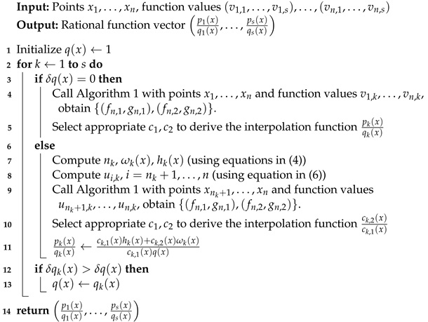
2.2. Fitzpatrick Algorithm for Univariate Vector-Valued Rational Interpolation

In the following, we discuss the univariate vector-valued rational interpolation problem where the denominators of different components share a common divisor, specifically, the vector-valued rational interpolation function in the form of (1).

Firstly, we use classical algorithms, such as the Fitzpatrick algorithm [12], the continued fraction method [13], or methods by solving linear systems of equations [14,15,16], to compute ${\displaystyle \frac{p_1\left(x\right)}{q_1\left(x\right)}}$. Then, computation of ${\displaystyle \frac{p_k\left(x\right)}{q_k\left(x\right)}}$ for $2\le k\le s$ can be conducted as follows. We first select $q_l\left(x\right)$ such that

$$\delta q_l\left(x\right)=\underset{1\le j\le k-1}{max}\left\{\delta q_j\left(x\right)\right\}.$$

(2)

If there are multiple polynomials satisfying (2), we choose the one with the largest index. Assuming that the greatest common divisor of $q_l\left(x\right)$ and $q_k\left(x\right)$ is ${\overline{q}}_k\left(x\right)$, there exist $s_{k,1}\left(x\right)$ and $s_{k,2}\left(x\right)$ such that $q_l\left(x\right)={\overline{q}}_k\left(x\right)·s_{k,1}\left(x\right)$ and $q_k\left(x\right)={\overline{q}}_k\left(x\right)·s_{k,2}\left(x\right)$. Therefore, ${\displaystyle \frac{p_k\left(x\right)}{q_k\left(x\right)}}$ can be expressed as

$${\displaystyle \frac{p_k\left(x\right)}{q_k\left(x\right)}}={\displaystyle \frac{s_{k,1}\left(x\right)p_k\left(x\right)}{q_l\left(x\right)s_{k,2}\left(x\right)}}.$$

Let ${\displaystyle \frac{a_k\left(x\right)}{b_k\left(x\right)}}={\displaystyle \frac{s_{k,1}\left(x\right)p_k\left(x\right)}{s_{k,2}\left(x\right)}}={\displaystyle \frac{p_k\left(x\right)}{q_k\left(x\right)}}·q_l\left(x\right)$. Then, we can establish a new rational interpolation problem:

$${\displaystyle \frac{a_k\left(x\right)}{b_k\left(x\right)}}{|}_{x=x_i}=v_{i,k}{q}_l\left(x_i\right),i=1,2,\dots ,n.$$

(3)

For the interpolation problem (3), we denote its corresponding weak interpolation module by ${\overline{M}}_k=\left\{(\tilde{a}\left(x\right),\tilde{b}\left(x\right))\right|\tilde{a}\left(x\right)-\tilde{b}\left(x\right)v_{i,k}{q}_l\left(x_i\right)\equiv 0mod{I}_i,i=1,2,\dots ,n\}$, where $I_i=⟨x-x_i⟩,i=1,2,\dots ,n$. Further, set

$$n_k=\delta q_l\left(x\right)+1\le n,h_k\left(x\right)=\sum _{i=1}^{n_k}{v}_{i,k}{q}_l\left(x_i\right)\prod _{\begin{array}{c}t=1\\ t\ne i\end{array}}^{n_k}{\displaystyle \frac{x-x_t}{x_i-x_t}},{\omega }_k\left(x\right)=\prod _{t=1}^{n_k}(x-x_t).$$

(4)

It can be easily verified that $\{(h_k\left(x\right),1),({\omega }_k\left(x\right),0)\}$ is a Gröbner basis for the module

$${\overline{M}}_{k,n_k}=\left\{(\overline{a}\left(x\right),\overline{b}\left(x\right))\right|\overline{a}\left(x\right)-\overline{b}\left(x\right)v_{i,k}{q}_l\left(x_i\right)\equiv 0mod{I}_i,i=1,\dots ,n_k\},$$

w.r.t. ${\prec }_{{\xi }_k}$, where ${\xi }_k=\delta h_k\left(x\right)$. Clearly, ${\overline{M}}_k\subset {\overline{M}}_{k,n_k}$, so for each $({\tilde{a}}_k\left(x\right),{\tilde{b}}_k\left(x\right))\in {\overline{M}}_k\subset {\overline{M}}_{k,n_k}$, there exist $c_{k,1}\left(x\right)$, $c_{k,2}\left(x\right)\in \mathbb{K}\left[x\right]$ such that

$$({\tilde{a}}_k\left(x\right),{\tilde{b}}_k\left(x\right))=c_{k,1}\left(x\right)·(h_k\left(x\right),1)+c_{k,2}\left(x\right)·({\omega }_k\left(x\right),0).$$

If $c_{k,1}\left(x\right)\ne 0$, the following expression is meaningful:

$${\displaystyle \frac{{\tilde{a}}_k\left(x\right)}{{\tilde{b}}_k\left(x\right)}}={\displaystyle \frac{c_{k,1}\left(x\right)h_k\left(x\right)+c_{k,2}\left(x\right){\omega }_k\left(x\right)}{c_{k,1}\left(x\right)·1}}.$$

(5)

Noting that $({\tilde{a}}_k\left(x\right),{\tilde{b}}_k\left(x\right))\in {\overline{M}}_k$, we also have

$${\displaystyle \frac{c_{k,1}\left(x_i\right)h_k\left(x_i\right)+c_{k,2}\left(x_i\right){\omega }_k\left(x_i\right)}{c_{k,1}\left(x_i\right)}}={\displaystyle \frac{{\tilde{a}}_k\left(x_i\right)}{{\tilde{b}}_k\left(x_i\right)}}=v_{i,k}{q}_l\left(x_i\right),i=n_k+1,\dots ,n.$$

Hence we can have

$${\displaystyle \frac{c_{k,2}\left(x\right)}{c_{k,1}\left(x\right)}}{|}_{x=x_i}=u_{i,k}={\displaystyle \frac{v_{i,k}{q}_l\left(x_i\right)-h_k\left(x_i\right)}{{\omega }_k\left(x_i\right)}},i=n_k+1,\dots ,n.$$

(6)

This represents a simpler rational interpolation problem. We can use the Fitzpatrick algorithm to solve this interpolation problem (6). Assuming that the solution is ${\displaystyle \frac{{\tilde{c}}_{k,2}\left(x\right)}{{\tilde{c}}_{k,1}\left(x\right)}}$, we substitute ${\tilde{c}}_{k,2}\left(x\right)$ and ${\tilde{c}}_{k,1}\left(x\right)$ into (5) and obtain ${\displaystyle \frac{{\tilde{a}}_k\left(x\right)}{{\tilde{b}}_k\left(x\right)}}$. Therefore,

$${\displaystyle \frac{p_k\left(x_i\right)}{q_k\left(x_i\right)}}={\displaystyle \frac{{\tilde{a}}_k\left(x_i\right)}{{\tilde{b}}_k\left(x_i\right)}}·{\displaystyle \frac{1}{q_l\left(x_i\right)}}={\displaystyle \frac{{\tilde{c}}_{k,1}\left(x_i\right)h_k\left(x_i\right)+{\tilde{c}}_{k,2}\left(x_i\right){\omega }_k\left(x_i\right)}{{\tilde{c}}_{k,1}\left(x_i\right)q_l\left(x_i\right)}}=v_{k,i},i=1,2,\cdots ,n.$$

Thus,

$${\displaystyle \frac{p_k\left(x\right)}{q_k\left(x\right)}}={\displaystyle \frac{{\tilde{c}}_{k,1}\left(x\right)h_k\left(x\right)+{\tilde{c}}_{k,2}\left(x\right){\omega }_k\left(x\right)}{{\tilde{c}}_{k,1}\left(x\right)q_l\left(x\right)}}$$

(7)

is the k-th component of the vector-valued rational interpolation function. Further observation shows that, if $\delta q_l\left(x\right)>0$, the degree of the rational function ${\displaystyle \frac{{\tilde{c}}_{k,2}\left(x\right)}{{\tilde{c}}_{k,1}\left(x\right)}}$ is lower than that of ${\displaystyle \frac{p_k\left(x\right)}{q_k\left(x\right)}}$. This property enables us to obtain a higher-degree rational function ${\displaystyle \frac{p_k\left(x\right)}{q_k\left(x\right)}}$ by computing the lower-degree rational interpolation function ${\displaystyle \frac{{\tilde{c}}_{k,2}\left(x\right)}{{\tilde{c}}_{k,1}\left(x\right)}}$. For specific implementation details, see Algorithm 2.

Remark 1. 

Due to the uncertainty of ${\displaystyle \frac{p_k\left(x\right)}{q_k\left(x\right)}}$, selecting $q_l\left(x\right)$ for maximum degree reduction is challenging. However, once the highest degree $q_l$ is chosen, the degree of the greatest common divisor between $q_k$ and $q_l$ may still be higher than that between $q_k$ and other denominators. From this perspective, this selection may not be optimal, but it remains reasonable.

Next, we compare our algorithm with the classical vector-valued rational interpolation algorithm in two aspects: the degree of the interpolation result and the approximation quality (see Examples 1 and 2). Since the majority of vector-valued rational interpolation algorithms are built upon the theory of the Thiele’s algorithm, i.e., the univariate Thiele vector-valued rational interpolation algorithm [6], we chose to compare our approach with the Thiele’s algorithm. To evaluate the accuracy of the interpolation, we introduce the following error metric: Let the interpolation function be $\overrightarrow{R}\left(x\right)=(r_1\left(x\right),r_2\left(x\right),\cdots ,r_s\left(x\right))$ and the original function be $\overrightarrow{V}\left(x\right)=(v_1\left(x\right),v_2\left(x\right),\cdots ,v_s\left(x\right))$. Then, the error for the k-th component is defined as $e_k\left(x\right)=r_k\left(x\right)-v_k\left(x\right)$. Consequently, the interpolation error vector can be expressed as

$$\overrightarrow{E}\left(x\right)=(e_1\left(x\right),e_2\left(x\right),\cdots ,e_s\left(x\right)).$$

In order to quantify the error further, we define the error bound as follows:

$$\mathrm{ERR}=\underset{1\le k\le s}{max}{E}_k,$$

(8)

where $E_k={max}_{a\le x\le b}\left|e_k\left(x\right)\right|$, for $k=1,2,\cdots ,s$, represents the error bound for the k-th component.

Algorithm 2: Fitzpatrick Algorithm for univariate vector-valued rational interpolation.

Example 1. 

Given the vector function $\left(\sqrt{x},-\sqrt{x^3}\right)$ and its data at the points $x_i$ as shown in Table 1, we seek a rational interpolation function that satisfies the data in the table.

Applying Algorithm 2, we then obtain the interpolation result as follows:

$$\left({\displaystyle \frac{15(x^2+15x+8)}{x^2+85x+274}},-{\displaystyle \frac{15x(x^2+15x+8)}{x^2+85x+274}}\right).$$

In contrast, the Thiele’s algorithm gives the following interpolation result:

$$\begin{array}{cc}\hfill & \left(-{\displaystyle \frac{15(352873x^4-16905050x^3+34618761x^2-9605868280x-8404972384)}{40877x^4-10728710x^3+514391421x^2+25851333460x+243536574152}},\right.\hfill \\ \hfill & \left.{\displaystyle \frac{15(2502965x^4-326370318x^3-6908154195x^2-15842123732x+5081371200)}{40877x^4-10728710x^3+514391421x^2+25851333460x+243536574152}}\right).\hfill \end{array}$$

By (8), the error bound for Algorithm 2 is calculated as $ER{R}_1=0.3044778370\times {10}^{-1}$, and the error bound for Thiele’s algorithm is $ER{R}_2=0.7349562562\times {10}^{-1}$. Furthermore, we present a graphical analysis contrasting the error functions of the results produced by both algorithms for each individual component, with detailed visualizations provided in Figure 1. Obviously, for this problem, Algorithm 2 outperforms the univariate Thiele’s algorithm in both solution degree and computational accuracy.

Table 1. Vector-valued rational interpolation data.

${\mathit{x}}_{\mathit{i}}$	${\mathit{x}}_1=1$	${\mathit{x}}_2=4$	${\mathit{x}}_3=9$	${\mathit{x}}_4=16$	${\mathit{x}}_5=25$
$(v_{i,1},v_{i,2})$	$(1,-1)$	$(2,-8)$	$(3,-27)$	$(4,-64)$	$(5,-125)$

Table 1. Vector-valued rational interpolation data.

${\mathit{x}}_{\mathit{i}}$	${\mathit{x}}_1=1$	${\mathit{x}}_2=4$	${\mathit{x}}_3=9$	${\mathit{x}}_4=16$	${\mathit{x}}_5=25$
$(v_{i,1},v_{i,2})$	$(1,-1)$	$(2,-8)$	$(3,-27)$	$(4,-64)$	$(5,-125)$

Figure 1. Comparison of interpolation result errors between the two algorithms.

Example 2. 

For the vector functions ${\overrightarrow{V}}_i\left(x\right)$ listed in Table 2, we sample the points at the provided knot sequences (denoted as $a:h:b$, which means a row vector starting from a and ending at b with step size h). Subsequently, we apply both Algorithm 2 and the univariate Thiele’s algorithm to calculate the interpolation functions and compare their approximation performance.

Using (8), we determine the error bounds with respect to the results of this problem for both Algorithm 2 and the univariate Thiele’s algorithm. These error bounds are presented in the 2nd and 3rd columns of Table 3, while the degrees of the interpolation functions are listed in the 4th and 5th columns. The data indicate that, in terms of both interpolation errors and function degrees, Algorithm 2 typically exhibits superior performance compared to the univariate Thiele’s algorithm for the current problem.

Table 2. Original functions and points.

i	${\overrightarrow{\mathit{V}}}_{\mathit{i}}\left(\mathit{x}\right)$	Knots
1	$\left({\displaystyle \frac{ln\left(x\right)}{x}},{\displaystyle \frac{e^x}{x}}\right)$	0.4:0.4:2.8
2	$\left({\displaystyle \frac{sin\left(x\right)}{{(x+1)}^2}},{\displaystyle \frac{cos\left(x\right)}{x(x+1)}}\right)$	0.2:0.2:1.4
3	$\left(\sqrt{{\displaystyle \frac{x-1}{{(x+1)}^3}}},\sqrt{{\displaystyle \frac{1}{x{(x+1)}^2}}},\sqrt{{\displaystyle \frac{x-1}{x(x+1)}}}\right)$	2.0:1.0:8.0
4	$\left(xsin\left(x\right),{\displaystyle \frac{cos\left(x\right)}{x}},tan\left(\sqrt{x}\right)\right)$	0.2:0.2:1.4
5	$\left(ln\left(x\right),tan\left(x\right),e^x,cos\left(x\right)\right)$	0.2:0.2:1.4
6	$\left(\sqrt{{\displaystyle \frac{x}{{(x+1)}^2}}},\sqrt{{\displaystyle \frac{x-1}{x^2(x+1)}}},\sqrt{{\displaystyle \frac{1}{x^2+1}}},\sqrt{{\displaystyle \frac{x-1}{x(x+1)}}}\right)$	3.0:1.0:9.0
7	$\left({\displaystyle \frac{ln\left(x\right)}{x+1}},\sqrt{{\displaystyle \frac{x}{x+1}}},sin\left(\sqrt{x}\right),\sqrt[3]{x^2+x},cos\left(\sqrt{x}\right)\right)$	0.2:0.2:1.4
8	$\left({\displaystyle \frac{ln(x-1)}{x^2+1}},e^{\sqrt{x}},\sqrt[3]{x^2+x},ln\left(\sqrt{x}\right),\sqrt{{\displaystyle \frac{x-1}{x^2+1}}}\right)$	2.0:1.0:8.0
9	$\left(x^3+x^2+x,sin\left(\sqrt{x}\right),\sqrt{{\displaystyle \frac{x}{x+1}}},cos\left(\sqrt{x}\right),\sqrt[3]{x^2+x},{\displaystyle \frac{e^x}{x+1}}\right)$	0.2:0.2:1.4
10	$\left({\displaystyle \frac{\sqrt{x}}{x^2+x}},\sqrt{{\displaystyle \frac{x}{x^2-1}}},\sqrt{x^3+1},{\displaystyle \frac{\sqrt{x}}{{(x+1)}^2}},\sqrt{{\displaystyle \frac{x-1}{x^2+x}}},\sqrt{x^2+x}\right)$	2.0:1.0:8.0

Table 2. Original functions and points.

i	${\overrightarrow{\mathit{V}}}_{\mathit{i}}\left(\mathit{x}\right)$	Knots
1	$\left({\displaystyle \frac{ln\left(x\right)}{x}},{\displaystyle \frac{e^x}{x}}\right)$	0.4:0.4:2.8
2	$\left({\displaystyle \frac{sin\left(x\right)}{{(x+1)}^2}},{\displaystyle \frac{cos\left(x\right)}{x(x+1)}}\right)$	0.2:0.2:1.4
3	$\left(\sqrt{{\displaystyle \frac{x-1}{{(x+1)}^3}}},\sqrt{{\displaystyle \frac{1}{x{(x+1)}^2}}},\sqrt{{\displaystyle \frac{x-1}{x(x+1)}}}\right)$	2.0:1.0:8.0
4	$\left(xsin\left(x\right),{\displaystyle \frac{cos\left(x\right)}{x}},tan\left(\sqrt{x}\right)\right)$	0.2:0.2:1.4
5	$\left(ln\left(x\right),tan\left(x\right),e^x,cos\left(x\right)\right)$	0.2:0.2:1.4
6	$\left(\sqrt{{\displaystyle \frac{x}{{(x+1)}^2}}},\sqrt{{\displaystyle \frac{x-1}{x^2(x+1)}}},\sqrt{{\displaystyle \frac{1}{x^2+1}}},\sqrt{{\displaystyle \frac{x-1}{x(x+1)}}}\right)$	3.0:1.0:9.0
7	$\left({\displaystyle \frac{ln\left(x\right)}{x+1}},\sqrt{{\displaystyle \frac{x}{x+1}}},sin\left(\sqrt{x}\right),\sqrt[3]{x^2+x},cos\left(\sqrt{x}\right)\right)$	0.2:0.2:1.4
8	$\left({\displaystyle \frac{ln(x-1)}{x^2+1}},e^{\sqrt{x}},\sqrt[3]{x^2+x},ln\left(\sqrt{x}\right),\sqrt{{\displaystyle \frac{x-1}{x^2+1}}}\right)$	2.0:1.0:8.0
9	$\left(x^3+x^2+x,sin\left(\sqrt{x}\right),\sqrt{{\displaystyle \frac{x}{x+1}}},cos\left(\sqrt{x}\right),\sqrt[3]{x^2+x},{\displaystyle \frac{e^x}{x+1}}\right)$	0.2:0.2:1.4
10	$\left({\displaystyle \frac{\sqrt{x}}{x^2+x}},\sqrt{{\displaystyle \frac{x}{x^2-1}}},\sqrt{x^3+1},{\displaystyle \frac{\sqrt{x}}{{(x+1)}^2}},\sqrt{{\displaystyle \frac{x-1}{x^2+x}}},\sqrt{x^2+x}\right)$	2.0:1.0:8.0

Remark 2. 

The computation of ${max}_{a\le x\le b}|r_k\left(x\right)-v_k\left(x\right)|$ is performed with built-in functions in Maple.

Example 3. 

Given

$$v_k\left(x\right)={\displaystyle \frac{x^{10(k-1)}+1}{x^{10(k-1)}(x^{10}+1)}},k=1,2,\cdots ,5,$$

let ${\overrightarrow{V}}_s\left(x\right)=(v_1\left(x\right),\cdots ,v_s\left(x\right))$, for $s=2,3,4$, and 5, be a set of vector-valued rational functions. We take $n=10,30,50$, and 70, respectively. Subsequently, we apply Algorithm 2 and the univariate Thiele’s algorithm to perform the calculations and record the respective runtime (in seconds) in detail.

For various values of n, the runtime of Algorithm 2 is presented in the 2nd, 4th, 6th, and 8th columns of Table 4, while the runtime of Thiele’s algorithm is shown in the 3rd, 5th, 7th, and 9th columns. It is evident from the data that, for this problem, for the same values of s and n, Algorithm 2 exhibits significantly less runtime than Thiele’s algorithm. Notably, as the number of sampling points, n, increases, the disparity in runtime between the two algorithms becomes increasingly pronounced.

Table 3. Comparison of degrees and errors between two algorithm results.

Function	ERR		Degree
	Algorithm 2	Thiele	Algorithm 2	Thiele
${\overrightarrow{V}}_1\left(x\right)$	$4.583114840\times {10}^{-4}$	$9.696897239\times {10}^{-3}$	$[5/4]$	$[6/6]$
${\overrightarrow{V}}_2\left(x\right)$	$9.327249980\times {10}^{-5}$	$1.280059824\times {10}^{-4}$	$[5/4]$	$[6/6]$
${\overrightarrow{V}}_3\left(x\right)$	$5.492107736\times {10}^{-6}$	$1.238846243\times {10}^{-5}$	$[6/4]$	$[6/6]$
${\overrightarrow{V}}_4\left(x\right)$	$1.804812124\times {10}^{-4}$	$3.450842263\times {10}^{-3}$	$[6/4]$	$[6/6]$
${\overrightarrow{V}}_5\left(x\right)$	$5.785323337\times {10}^{-4}$	$6.187137002\times {10}^{-3}$	$[6/4]$	$[6/6]$
${\overrightarrow{V}}_6\left(x\right)$	$5.620278566\times {10}^{-7}$	$4.105675605\times {10}^{-6}$	$[6/4]$	$[6/6]$
${\overrightarrow{V}}_7\left(x\right)$	$1.487813369\times {10}^{-5}$	$2.560689242\times {10}^{-4}$	$[6/4]$	$[6/6]$
${\overrightarrow{V}}_8\left(x\right)$	$2.229500738\times {10}^{-4}$	$1.057572358\times {10}^{-3}$	$[6/4]$	$[6/6]$
${\overrightarrow{V}}_9\left(x\right)$	$6.480739393\times {10}^{-5}$	$1.951852363\times {10}^{-4}$	$[6/4]$	$[6/6]$
${\overrightarrow{V}}_{10}\left(x\right)$	$4.813018968\times {10}^{-5}$	$3.718845805\times {10}^{-4}$	$[6/4]$	$[6/6]$

Table 3. Comparison of degrees and errors between two algorithm results.

Function	ERR		Degree
	Algorithm 2	Thiele	Algorithm 2	Thiele
${\overrightarrow{V}}_1\left(x\right)$	$4.583114840\times {10}^{-4}$	$9.696897239\times {10}^{-3}$	$[5/4]$	$[6/6]$
${\overrightarrow{V}}_2\left(x\right)$	$9.327249980\times {10}^{-5}$	$1.280059824\times {10}^{-4}$	$[5/4]$	$[6/6]$
${\overrightarrow{V}}_3\left(x\right)$	$5.492107736\times {10}^{-6}$	$1.238846243\times {10}^{-5}$	$[6/4]$	$[6/6]$
${\overrightarrow{V}}_4\left(x\right)$	$1.804812124\times {10}^{-4}$	$3.450842263\times {10}^{-3}$	$[6/4]$	$[6/6]$
${\overrightarrow{V}}_5\left(x\right)$	$5.785323337\times {10}^{-4}$	$6.187137002\times {10}^{-3}$	$[6/4]$	$[6/6]$
${\overrightarrow{V}}_6\left(x\right)$	$5.620278566\times {10}^{-7}$	$4.105675605\times {10}^{-6}$	$[6/4]$	$[6/6]$
${\overrightarrow{V}}_7\left(x\right)$	$1.487813369\times {10}^{-5}$	$2.560689242\times {10}^{-4}$	$[6/4]$	$[6/6]$
${\overrightarrow{V}}_8\left(x\right)$	$2.229500738\times {10}^{-4}$	$1.057572358\times {10}^{-3}$	$[6/4]$	$[6/6]$
${\overrightarrow{V}}_9\left(x\right)$	$6.480739393\times {10}^{-5}$	$1.951852363\times {10}^{-4}$	$[6/4]$	$[6/6]$
${\overrightarrow{V}}_{10}\left(x\right)$	$4.813018968\times {10}^{-5}$	$3.718845805\times {10}^{-4}$	$[6/4]$	$[6/6]$

Table 4. Comparison of runtime between two algorithms.

s	n = 10		n = 30		n = 50		n = 70
	Algorithm 2	Thiele	Algorithm 2	Thiele	Algorithm 2	Thiele	Algorithm 2	Thiele
2	0.015000	0.016000	0.062000	1.265000	0.328000	13.750000	1.578000	95.891000
3	0.016000	0.032000	0.141000	2.422000	1.391000	28.281000	10.640000	196.828000
4	0.031000	0.047000	0.250000	4.078000	4.109000	51.172000	40.469000	318.484000
5	0.032000	0.047000	0.563000	4.968000	7.938000	70.453000	108.813000	432.188000

Table 4. Comparison of runtime between two algorithms.

s	n = 10		n = 30		n = 50		n = 70
	Algorithm 2	Thiele	Algorithm 2	Thiele	Algorithm 2	Thiele	Algorithm 2	Thiele
2	0.015000	0.016000	0.062000	1.265000	0.328000	13.750000	1.578000	95.891000
3	0.016000	0.032000	0.141000	2.422000	1.391000	28.281000	10.640000	196.828000
4	0.031000	0.047000	0.250000	4.078000	4.109000	51.172000	40.469000	318.484000
5	0.032000	0.047000	0.563000	4.968000	7.938000	70.453000	108.813000	432.188000

Remark 3. 

All computations in this paper are performed on a hardware environment equipped with a 64-bit 1.8 GHz Intel Core i7 processor and 8 GB of RAM, Windows 10 Enterprise operating system and Maple 2016.

3. Univariate Vector-Valued Rational Recovery

In this section, we discuss an application of univariate vector-valued rational interpolation, specifically focusing on the problem of recovering univariate vector-valued rational functions. Let $\overrightarrow{V}\left(x\right)=(v_1\left(x\right),v_2\left(x\right),\cdots ,v_s\left(x\right))$ be a univariate vector-valued rational function provided by a black box $B:\mathbb{R}\to {\mathbb{R}}^s$ with an unknown specific form. Once some $x_i\in \mathbb{R}$ is input, the black box outputs the function value $\overrightarrow{V}\left(x_i\right)\in {\mathbb{R}}^s$. Suppose the black box function gives sufficient data

$$\{(x_i,{\overrightarrow{V}}_i):x_i\in \mathbb{R};{\overrightarrow{V}}_i=\overrightarrow{V}\left(x_i\right)=(v_1\left(x_i\right),v_2\left(x_i\right),\cdots ,v_s\left(x_i\right))=(v_{i,1},\dots ,v_{i,s})\in {\mathbb{R}}^s;i=1,2,\dots ,N\},$$

we aim to reconstruct a vector-valued rational function

$$\overrightarrow{R}\left(x\right)=\left({\displaystyle \frac{p_1\left(x\right)}{q_1\left(x\right)}},{\displaystyle \frac{p_2\left(x\right)}{q_2\left(x\right)}},\dots ,{\displaystyle \frac{p_s\left(x\right)}{q_s\left(x\right)}}\right),$$

such that

$$\overrightarrow{R}\left(x_i\right)=\overrightarrow{V}\left(x_i\right),i=1,2,\dots ,N,$$

where for all $1\le i\le s$, $\delta p_i\le l$, $\delta q_i\le m$, and $l+m<N$. In this case, we consider $\overrightarrow{R}\left(x\right)$ to be the function obtained by recovering $\overrightarrow{V}\left(x\right)$.

A common approach to solving this problem involves two procedures: applying a recursive vector-valued rational interpolation algorithm to compute ${\overrightarrow{R}}_k\left(x\right)$ for $k=1,2,\cdots ,N$ and verifying if it equals $\overrightarrow{V}\left(x\right)$ at all data points. However, this handling method suffers from computational redundancy.

To reduce computational redundancy, we propose a novel strategy to deal with the recovery of vector-valued rational functions. Specifically, we sample at two distinct sets of points with the black-box function $\overrightarrow{V}\left(x\right)$: a computation set $J_1=\{x_i:i=1,2,\dots ,t\}$, where t is adjustable; and a validation set $J_2=\{{\tilde{x}}_1,{\tilde{x}}_2\}$, where ${\tilde{x}}_1$ and ${\tilde{x}}_2$ are large prime numbers. On $J_1$, we apply a recursive vector-valued rational interpolation algorithm to compute the k-th component ${\displaystyle \frac{p_{t,k}\left(x\right)}{q_{t,k}\left(x\right)}}$ of the interpolation function. Subsequently, on $J_2$, we verify if ${\displaystyle \frac{p_{t,k}\left(x\right)}{q_{t,k}\left(x\right)}}$ equals $v_k\left(x\right)$. If ${\displaystyle \frac{p_{t,k}\left({\tilde{x}}_i\right)}{q_{t,k}\left({\tilde{x}}_i\right)}}=v_k\left({\tilde{x}}_i\right)$ holds for $i=1,2$, we consider that the k-th component is successfully recovered and proceed to compute the $(k+1)$-th component with the same method. Otherwise, we increase the number of points and continue to compute ${\displaystyle \frac{p_{t+1,k}\left(x\right)}{q_{t+1,k}\left(x\right)}}$ based on ${\displaystyle \frac{p_{t,k}\left(x\right)}{q_{t,k}\left(x\right)}}$. As our algorithm processes each component individually, we can modify Algorithm 2 accordingly to implement this procedure, which yields Algorithm 3, as follows.

Algorithm 3: Fitzpatrick Algorithm for univariate vector-valued rational recovery.

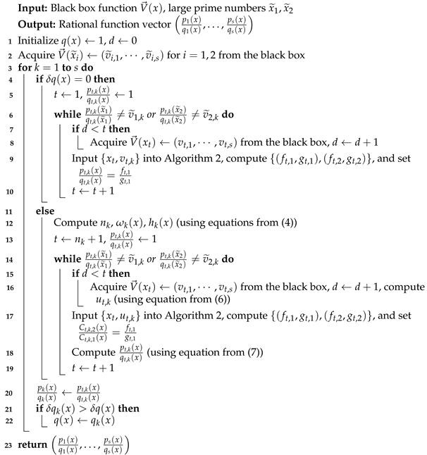
Next, we will select several sets of black box functions to test Algorithm 3. Additionally, we will compare its performance with a vector-valued rational recovery algorithm, which is derived from Thiele’s algorithm together with the termination conditions (referred to as the Thiele-type algorithm).

Example 4. 

Let the black box rational function be $\overrightarrow{V}\left(x\right)=\left({\displaystyle \frac{x+1}{2x^2+2}},-{\displaystyle \frac{x-1}{(x+1)(x^2+1)}}\right)$. We perform rational recovery with Algorithm 3.

(1) Choose two large prime numbers at random. Let ${\tilde{x}}_1=7717$, ${\tilde{x}}_2=7907$, and obtain the function values

$$\overrightarrow{V}\left({\tilde{x}}_1\right)=\left({\displaystyle \frac{3859}{59552090}},-{\displaystyle \frac{1929}{114905757655}}\right),\overrightarrow{V}\left({\tilde{x}}_2\right)=\left({\displaystyle \frac{1977}{31260325}},-{\displaystyle \frac{3953}{247206650100}}\right).$$

(2) Select points $x_t=t,t=1,2,\cdots ,20$, and input the points $x_t$ sequentially into Algorithm 2 for interpolation. For $t=5$, we have ${\displaystyle \frac{p_{5,1}\left(x\right)}{q_{5,1}\left(x\right)}}={\displaystyle \frac{1}{2}}·{\displaystyle \frac{x+1}{x^2+1}}$. One can easily check that ${\displaystyle \frac{p_{5,1}\left({\tilde{x}}_1\right)}{q_{5,1}\left({\tilde{x}}_1\right)}}={\displaystyle \frac{3859}{59552090}}={\tilde{v}}_{1,1}$ and ${\displaystyle \frac{p_{5,1}\left({\tilde{x}}_2\right)}{q_{5,1}\left({\tilde{x}}_2\right)}}={\displaystyle \frac{1977}{31260325}}={\tilde{v}}_{2,1}$, then ${\displaystyle \frac{p_1\left(x\right)}{q_1\left(x\right)}}={\displaystyle \frac{p_{5,1}\left(x\right)}{q_{5,1}\left(x\right)}}={\displaystyle \frac{1}{2}}·{\displaystyle \frac{x+1}{x^2+1}}$ (data used is shown in Table 5).

(3) Let $q\left(x\right)=2x^2+2$, then we obtain $n_2=3$, ${\omega }_2\left(x\right)=(x-1)(x-2)(x-3)$, $h_2\left(x\right)={\displaystyle \frac{1}{6}}{x}^2-{\displaystyle \frac{7}{6}}x+1$.

For $t=4,5,\cdots ,20$, input the points $x_t$ sequentially, calculate $u_{t,2}$, and interpolate ${\displaystyle \frac{{\tilde{c}}_{t,2,2}\left(x\right)}{{\tilde{c}}_{t,2,1}\left(x\right)}}$ with Algorithm 2, then compute ${\displaystyle \frac{p_{t,2}\left(x\right)}{q_{t,2}\left(x\right)}}$. For $t=6$, we have ${\displaystyle \frac{{\tilde{c}}_{6,2,2}\left(x\right)}{{\tilde{c}}_{6,2,1}\left(x\right)}}=-{\displaystyle \frac{1}{6(x+1)}}$, and then compute ${\displaystyle \frac{p_{6,2}\left(x\right)}{q_{6,2}\left(x\right)}}=-{\displaystyle \frac{x-1}{(x+1)(x^2+1)}}$ which satisfies ${\displaystyle \frac{p_{6,2}\left({\tilde{x}}_1\right)}{q_{6,2}\left({\tilde{x}}_1\right)}}=-{\displaystyle \frac{1929}{114905757655}}={\tilde{v}}_{1,2}$ and ${\displaystyle \frac{p_{6,2}\left({\tilde{x}}_2\right)}{q_{6,2}\left({\tilde{x}}_2\right)}}=-{\displaystyle \frac{3953}{247206650100}}={\tilde{v}}_{2,2}$, thus ${\displaystyle \frac{p_2\left(x\right)}{q_2\left(x\right)}}={\displaystyle \frac{p_{6,2}\left(x\right)}{q_{6,2}\left(x\right)}}=-{\displaystyle \frac{x-1}{(x+1)(x^2+1)}}$ (data used are shown in Table 5).

Finally, the rational recovery result is

$$\overrightarrow{R}\left(x\right)=\left({\displaystyle \frac{x+1}{2x^2+2}},-{\displaystyle \frac{x-1}{(x+1)(x^2+1)}}\right).$$

Table 5. Vector-valued rational restoration data.

${\mathit{x}}_{\mathit{i}}$	${\mathit{x}}_1=1$	${\mathit{x}}_2=2$	${\mathit{x}}_3=3$	${\mathit{x}}_4=4$	${\mathit{x}}_5=5$	${\mathit{x}}_6=6$
$\overrightarrow{V}\left(x_i\right)$	$\left({\displaystyle \frac{1}{2}},0\right)$	$\left({\displaystyle \frac{3}{10}},-{\displaystyle \frac{1}{15}}\right)$	$\left({\displaystyle \frac{1}{5}},-{\displaystyle \frac{1}{20}}\right)$	$\left({\displaystyle \frac{5}{34}},-{\displaystyle \frac{3}{85}}\right)$	$\left({\displaystyle \frac{3}{26}},-{\displaystyle \frac{1}{39}}\right)$	$\left({\displaystyle \frac{7}{74}},-{\displaystyle \frac{5}{259}}\right)$

Table 5. Vector-valued rational restoration data.

${\mathit{x}}_{\mathit{i}}$	${\mathit{x}}_1=1$	${\mathit{x}}_2=2$	${\mathit{x}}_3=3$	${\mathit{x}}_4=4$	${\mathit{x}}_5=5$	${\mathit{x}}_6=6$
$\overrightarrow{V}\left(x_i\right)$	$\left({\displaystyle \frac{1}{2}},0\right)$	$\left({\displaystyle \frac{3}{10}},-{\displaystyle \frac{1}{15}}\right)$	$\left({\displaystyle \frac{1}{5}},-{\displaystyle \frac{1}{20}}\right)$	$\left({\displaystyle \frac{5}{34}},-{\displaystyle \frac{3}{85}}\right)$	$\left({\displaystyle \frac{3}{26}},-{\displaystyle \frac{1}{39}}\right)$	$\left({\displaystyle \frac{7}{74}},-{\displaystyle \frac{5}{259}}\right)$

Example 5. 

Given

$$v_k\left(x\right)={\displaystyle \frac{x^{k+1}+1}{(x^k+1)(x^5+x+1)}},k=0,1,2,\cdots ,6,$$

let ${\overrightarrow{V}}_s\left(x\right)=(v_0\left(x\right),\cdots ,v_s\left(x\right))$, for $s=1,2,\cdots ,6$, be a set of black box vector-valued rational functions.

We compute the recovery of rational functions using both Algorithm 3 and the Thiele-type algorithm. First, two large prime numbers, ${\tilde{x}}_1=3167$ and ${\tilde{x}}_2=3319$, are selected and their corresponding function values are obtained. Additionally, points $x_i=i$ for $i=1,2,\cdots ,50$, are selected and input into the algorithms. Table 6 lists the number of points and runtime consumed by Algorithm 3 in the 2nd and 4th columns, respectively. The respective information for the Thiele-type algorithm is presented in the 3rd and 5th columns. As the vector dimension increases, the experimental results show that, in this problem, Algorithm 3 exhibits significant advantages over the Thiele-type algorithm in terms of both runtime and the number of points required.

Table 6. Comparison of points and runtime between the two algorithms.

Function	Number of Points		Runtime (s)
	Algorithm 3	Thiele	Algorithm 3	Thiele
${\overrightarrow{V}}_1\left(x\right)$	11	13	0.015	0.063
${\overrightarrow{V}}_2\left(x\right)$	12	17	0.016	0.219
${\overrightarrow{V}}_3\left(x\right)$	15	21	0.016	0.797
${\overrightarrow{V}}_4\left(x\right)$	18	29	0.016	5.453
${\overrightarrow{V}}_5\left(x\right)$	21	37	0.032	28.125
${\overrightarrow{V}}_6\left(x\right)$	24	45	0.062	115.907

If there are no non-trivial common divisors among the denominators of the components, such as

$$\left({\displaystyle \frac{x+1}{x^2+1}},-{\displaystyle \frac{x^3+x}{x^4+3}},x^2+1,-{\displaystyle \frac{2}{x^6+2x}}\right),$$

Algorithm 3 can still successfully recover these functions. This fully demonstrates the versatility and effectiveness of Algorithm 3, indicating that it is not only applicable to specific cases where the denominators of vector-valued interpolation functions have non-trivial common divisors, but also widely applicable to general vector-valued rational function recovery problems.

Next, we consider the application of the vector-valued rational recovery algorithm in solving positive-dimensional polynomial systems. Let I be a given positive-dimensional ideal, and suppose that a maximally independent set modulo I is $U=(x_1,\cdots ,x_d)$. Let $V=X\setminus U=(x_{d+1},\cdots ,x_n)$. Denote the extension of I over $\mathbb{K}\left(U\right)$ by $I^e$, then $I^e\subset \mathbb{K}\left(U\right)\left[V\right]$ is a 0 dimensional ideal over $\mathbb{K}\left(U\right)\left[V\right]$. According to the reference [17], solving for $I^e$ is the most critical step in solving positive-dimensional polynomial systems. Therefore, we focus on discussing the solution process of $I^e$ here. Let t be the separating element of the extension ideal $I^e\subset \mathbb{K}\left(U\right)\left[V\right]$. According to the RUR (Rational Univariate Representation) method for polynomial systems [18], the solutions of $I^e$ can be represented by a set of univariate polynomials over $\mathbb{K}\left(U\right)$ in terms of T:

$$\{{\chi }_t\left(T\right),G_t(1,T),G_t(x_{d+1},T),\dots ,G_t(x_n,T)\}.$$

That is, the solutions of I can be expressed as

$${\chi }_t\left(T\right)=0,G_t(1,T)\ne 0,x_1=x_1,\dots ,x_d=x_d,x_{d+1}={\displaystyle \frac{G_t(x_{d+1},T)}{G_t(1,T)}},\dots ,x_n={\displaystyle \frac{G_t(x_n,T)}{G_t(1,T)}}.$$

The coefficients of these univariate polynomials are rational functions over $\mathbb{K}\left(U\right)$, which need to be computed. To this end, let $\overrightarrow{R}\left(U\right)$ be the vector composed of all coefficients of these polynomials:

$$\overrightarrow{R}\left(U\right)=\left({\displaystyle \frac{p_1\left(U\right)}{q_1\left(U\right)}},{\displaystyle \frac{p_2\left(U\right)}{q_2\left(U\right)}},\dots ,{\displaystyle \frac{p_s\left(U\right)}{q_s\left(U\right)}}\right).$$

Direct symbolic computations of these rational functions are computationally expensive. To compute these rational functions, we select appropriate points $U_i\in {\mathbb{K}}^d$, and evaluate the generators of I at these points to obtain zero-dimensional ideals $I_{U_i}$. Under certain conditions, t remains to be the separating element of the zero-dimensional ideal $I_{U_i}$. Then, RUR of $I_{U_i}$ is calculated as follows:

$$\{{\chi }_t\left(T\right){|}_{U_i},{\mathfrak{g}}_{t,1}^{U_i}\left(T\right),{\mathfrak{g}}_{t,x_{i_{d+1}}}^{U_i}\left(T\right),\dots ,{\mathfrak{g}}_{t,x_{i_n}}^{U_i}\left(T\right)\}.$$

These are univariate polynomials over $\mathbb{K}$ in terms of T. According to reference [17], under appropriate conditions, ${\mathfrak{g}}_{t,h}^{U_i}\left(T\right)=G_t{(h,T)|}_{U=U_i}$, and if the vector of their coefficients is

$${\overrightarrow{V}}_i=(v_{i,1},\dots ,v_{i,s}),$$

then

$$v_{i,j}={\displaystyle \frac{p_j\left(U_i\right)}{q_j\left(U_i\right)}},j=1,\dots ,s.$$

This is equivalent to obtaining the values of the rational functions ${\displaystyle \frac{p_j\left(U\right)}{q_j\left(U\right)}}$, $j=1,2,\dots ,s$, at the points $U_i$. By applying the previous rational function recovery method, we can obtain ${\displaystyle \frac{p_j\left(U\right)}{q_j\left(U\right)}}$, $j=1,2,\dots ,s$.

In the following examples, we incorporate the vector-valued rational function recovery method into the algorithm described in [17] in order to obtain solutions to polynomial systems.

Example 6. 

Given

$$\begin{array}{cc}\hfill I=& ⟨x_1+x_2+x_3+x_4,x_1{x}_2+x_2{x}_3+x_1{x}_4+x_3{x}_4,\hfill \\ \hfill & x_1{x}_2{x}_3+x_1{x}_2{x}_4+x_1{x}_3{x}_4+x_2{x}_3{x}_4,x_1{x}_2{x}_3{x}_4-1⟩,\hfill \end{array}$$

where I is a positive-dimensional ideal, and the maximally independent set modulo I is $U=\left\{x_1\right\}$, thus $V=\{x_2,x_3,x_4\}$. We first arbitrarily select two large prime numbers, ${\tilde{U}}_1=7433$ and ${\tilde{U}}_2=8011$, to obtain function values. We then choose points $U_i=i$ for $i=1,2,\cdots ,10$, and substitute $x_1=U_i$ into the ideal I to obtain $I_{U_i}$. Taking $t=x_2$ as the separating element, we obtain the RUR of $I_{U_i}$ as follows:

$$\left\{{\chi }_t^{U_i}\left(T\right)=T^2+v_{i,1},{\mathfrak{g}}_{t,1}^{U_i}\left(T\right)=2T,{\mathfrak{g}}_{t,x_2}^{U_i}\left(T\right)=v_{i,2},{\mathfrak{g}}_{t,x_3}^{U_i}\left(T\right)=v_{i,3}T,{\mathfrak{g}}_{t,x_4}^{U_i}\left(T\right)=v_{i,4}\right\},$$

and then extract the coefficients to form the vector

$${\overrightarrow{V}}_i=\left(v_{i,1},v_{i,2},v_{i,3},v_{i,4}\right),$$

which represents the function values at point $U_i$. The relevant data at point $U_i$ are then input into the interpolation algorithm, and ${\tilde{U}}_1$ and ${\tilde{U}}_2$ are used for validation; the data for recovery are presented in Table 7.

The recovered result is

$$\overrightarrow{V}\left(x_1\right)=\left(-{\displaystyle \frac{1}{x_1^2}},{\displaystyle \frac{2}{x_1^2}},-2x_1,-{\displaystyle \frac{2}{x_1^2}}\right).$$

This solution agrees with the one obtained using a different method in reference [19].

Table 7. Coefficient data of RUR of $I_{U_i}$.

i	${\mathit{U}}_{\mathit{i}}$	${\overrightarrow{\mathit{V}}}_{\mathit{i}}$
1	3	$\left(-{\displaystyle \frac{1}{9}},{\displaystyle \frac{2}{9}},-6,-{\displaystyle \frac{2}{9}}\right)$
2	5	$\left(-{\displaystyle \frac{1}{25}},{\displaystyle \frac{2}{25}},-10,-{\displaystyle \frac{2}{25}}\right)$
3	7	$\left(-{\displaystyle \frac{1}{49}},{\displaystyle \frac{2}{49}},-14,-{\displaystyle \frac{2}{49}}\right)$
4	9	$\left(-{\displaystyle \frac{1}{81}},{\displaystyle \frac{2}{81}},-18,-{\displaystyle \frac{2}{81}}\right)$
5	11	$\left(-{\displaystyle \frac{1}{121}},{\displaystyle \frac{2}{121}},-22,-{\displaystyle \frac{2}{121}}\right)$

Table 7. Coefficient data of RUR of $I_{U_i}$.

i	${\mathit{U}}_{\mathit{i}}$	${\overrightarrow{\mathit{V}}}_{\mathit{i}}$
1	3	$\left(-{\displaystyle \frac{1}{9}},{\displaystyle \frac{2}{9}},-6,-{\displaystyle \frac{2}{9}}\right)$
2	5	$\left(-{\displaystyle \frac{1}{25}},{\displaystyle \frac{2}{25}},-10,-{\displaystyle \frac{2}{25}}\right)$
3	7	$\left(-{\displaystyle \frac{1}{49}},{\displaystyle \frac{2}{49}},-14,-{\displaystyle \frac{2}{49}}\right)$
4	9	$\left(-{\displaystyle \frac{1}{81}},{\displaystyle \frac{2}{81}},-18,-{\displaystyle \frac{2}{81}}\right)$
5	11	$\left(-{\displaystyle \frac{1}{121}},{\displaystyle \frac{2}{121}},-22,-{\displaystyle \frac{2}{121}}\right)$

SHEPWM (Selective Harmonic Elimination Pulse Width Modulation) stands as a vital technology in medium- and high-voltage, high-power inverters, characterized not only by low switching losses but also by its ability to achieve linear control of the fundamental voltage to optimize the quality of the output voltage. Harmonic elimination theory allows us to derive a set of trigonometric algebraic equations with N switching angles, known as the SHEPWM equations. In 2004, Chiasson et al. [20] were the first to attempt transforming such trigonometric algebraic equations into a polynomial system for solution. In 2017, Shang et al. [21] further simplified these polynomial systems and proposed a method for solving them with the rational representation theory of positive-dimensional ideals.

Example 7. 

The SHEPWM problem with $N=3$ can be solved by finding the zeros of the ideal

$$\begin{array}{cc}\hfill I:=& ⟨{\displaystyle \frac{1}{5}}{s}_1^5-s_1^3{s}_2-s_1^3+s_1^2{s}_3+s_1{s}_2^2+3s_1{s}_2-s_2{s}_3+s_1-3s_3,\hfill \\ \hfill & {\displaystyle \frac{1}{7}}{s}_1^7-s_1^5{s}_2-s_1^5+s_1^4{s}_3+2s_1^3{s}_2^2+5s_1^3{s}_2-3s_1^2{s}_2{s}_3-s_1{s}_2^3+2s_1^3\hfill \\ \hfill & -5s_1^2{s}_3-5s_1{s}_2^2+s_1{s}_3^2+s_2^2{s}_3-6s_1{s}_2+5s_2{s}_3-s_1+6s_3⟩,\hfill \end{array}$$

where I is a positive-dimensional ideal, and the maximally independent set modulo I is $U=\left\{s_1\right\}$ and $V=\{s_2,s_3\}$. We first select two large prime numbers, ${\tilde{U}}_1=7001$ and ${\tilde{U}}_2=8009$, to obtain function values. Choosing $U_i=i$ for $i=1,\dots ,30$, and taking $t=s_2$ as the separating element, we obtain the RUR of $I_{U_i}$ as follows:

$$\begin{array}{cc}\hfill & \{{\chi }_t^{U_i}\left(T\right)=T^3+v_{i,1}{T}^2+v_{i,2}T+v_{i,3},{\mathfrak{g}}_{t,1}^{U_i}\left(T\right)=3T^2+v_{i,4}T+v_{i,5},\hfill \\ \hfill & {\mathfrak{g}}_{t,s_2}^{U_i}\left(T\right)=v_{i,6}{T}^2+v_{i,7}T+v_{i,8},{\mathfrak{g}}_{t,s_3}^{U_i}\left(T\right)=v_{i,9}{T}^2+v_{i,10}T+v_{i,11}\},\hfill \end{array}$$

all the coefficients form the vector

$${\overrightarrow{V}}_i=\left(v_{i,1},v_{i,2},v_{i,3},v_{i,4},v_{i,5},v_{i,6},v_{i,7},v_{i,8},v_{i,9},v_{i,10},v_{i,11}\right),$$

which represents the function values at point $U_i$. The relevant data at point $U_i$ are then input into the interpolation algorithm, and ${\tilde{U}}_1$ and ${\tilde{U}}_2$ are used for validation. The data used for recovery are provided in Appendix A. The recovered result is

$$\begin{array}{cc}\hfill & \overrightarrow{V}\left(U\right)=(-{\displaystyle \frac{9s_1^6-91s_1^4+280s_1^2-245}{7(s_1^4-5s_1^2+5)}},{\displaystyle \frac{(s_1^3-3)(4s_1^6-49s_1^4+175s_1^2-175)}{7(s_1^4-5s_1^2+5)}},\hfill \\ \hfill & -{\displaystyle \frac{(3s_1^{10}-60s_1^8+440s_1^6-1505s_1^4+2450s_1^2-1575)}{35(s_1^4-5s_1^2+5)}},-{\displaystyle \frac{2(9s_1^6-91s_1^4+280s_1^2-245)}{7(s_1^4-5s_1^2+5)}},\hfill \\ \hfill & {\displaystyle \frac{4s_1^8-61s_1^6+322s_1^4-700s_1^2+525}{7(s_1^4-5s_1^2+5)}},{\displaystyle \frac{9s_1^6-91s_1^4+280s_1^2-245}{7(s_1^4-5s_1^2+5)}},\hfill \\ \hfill & -{\displaystyle \frac{2(4s_1^8-61s_1^6+322s_1^4-700s_1^2+525)}{7(s_1^4-5s_1^2+5)}},{\displaystyle \frac{9s_1^{10}-180s_1^8+1320s_1^6-4515s_1^4+7350s_1^2-4725}{35(s_1^4-5s_1^2+5)}},\hfill \\ \hfill & {\displaystyle \frac{s_1(2s_1^6-35s_1^4+140s_1^2-140)}{7(s_1^4-5s_1^2+5)}},-{\displaystyle \frac{3s_1(3s_1^8-65s_1^6+420s_1^4-1050s_1^2+875)}{35(s_1^4-5s_1^2+5)}},\hfill \\ \hfill & {\displaystyle \frac{s_1(2s_1^{10}-51s_1^8+440s_1^6-1715s_1^4+3150s_1^2-2275)}{35(s_1^4-5s_1^2+5)}}).\hfill \end{array}$$

The solution obtained from this result agrees with the one found using a different method in reference [21].

4. Conclusions

This paper deals with the problems of univariate vector-valued rational interpolation and recovery with common divisors in the denominators. We propose a univariate vector-valued rational interpolation algorithm that takes the advantage of the property of a common divisor.Specifically, it leverages the denominators obtained from prior interpolated components to reduce the degree of interpolation for subsequent ones. By incorporating termination conditions into this algorithm, a vector-valued rational recovery algorithm can be derived. Numerical experiments demonstrate reliable performance of the algorithm in interpolation and recovery, offering advantages over traditional univariate Thiele-type algorithms. Additionally, we explore its application in solving positive-dimensional polynomial systems, confirming its feasibility in practical scenarios. However, when we are confronted with bivariate or multivariate vector-valued rational interpolation problems, the construction of the algorithm encounters greater challenges due to the complexity of interpolation points and function definitions. Future work aims to further investigate solutions for bivariate vector-valued rational interpolation and recovery, specifically targeting these more complex scenarios. In our research, we find in [22] that interpolation calculations can be applied to the solution of differential equations [23]. Consequently, we plan to use our method to solve differential equations in the future. We discover that in [24], the idea of mapping is utilized in the process of solving the problem, and the method we propose in this paper for solving positive-dimensional ideal problems actually establishes a homomorphic image mapping between solutions in zero-dimensional space and positive-dimensional space. This sparks our interest in using mappings to solve problems. Therefore, our next step is to explore the application of this mapping concept in solving different types of problems.

References

- Graves-Morris, P.R.; Beckermann, B. The compass (star) identity for vector-valued rational interpolants. Adv. Comput. Math. 1997, 7, 279–294. [Google Scholar] [CrossRef]
- Wu, B.; Li, Z.; Li, S. The implementation of a vector-valued rational approximate method in structural reanalysis problems. Comput. Methods Appl. Mech. Eng. 2003, 192, 1773–1784. [Google Scholar] [CrossRef]
- Tsekeridou, S.; Cheikh, F.A.; Gabbouj, M.; Pitas, I. Vector rational interpolation schemes for erroneous motion field estimation applied to MPEG-2 error concealment. IEEE Trans. Multimed. 2004, 6, 876–885. [Google Scholar] [CrossRef]
- Hu, G.; Qin, X.; Ji, X.; Wei, G.; Zhang, S. The construction of λμ-B-spline curves and its application to rotational surfaces. Appl. Math. Comput. 2015, 266, 194–211. [Google Scholar] [CrossRef]
- He, L.; Tan, J.; Huo, X.; Xie, C. A novel super-resolution image and video reconstruction approach based on Newton-Thiele’s rational kernel in sparse principal component analysis. Multimed. Tools Appl. 2017, 76, 9463–9483. [Google Scholar] [CrossRef]
- Graves-Morris, P.R. Vector valued rational interpolants I. Numer. Math. 1983, 42, 331–348. [Google Scholar] [CrossRef]
- Graves-Morris, P.R. Vector-valued rational interpolants II. IMA J. Numer. Anal. 1984, 4, 209–224. [Google Scholar] [CrossRef]
- Graves-Morris, P.R.; Jenkins, C.D. Vector-valued rational interpolants III. Constr. Approx. 1986, 2, 263–289. [Google Scholar] [CrossRef]
- Levrie, P.; Bultheel, A. A note on thiele n-fractions. Numer. Algor. 1993, 4, 225–239. [Google Scholar] [CrossRef]
- Zhu, X.; Zhu, G. A recurrence algorithm for vector valued rational interpolation. J. Univ. Sci. Technol. China 2003, 33, 15–25. [Google Scholar] [CrossRef]
- Wang, R.; Zhu, G. Rational Function Approximation and Its Applications; Science Press: Beijing, China, 2004; pp. 117–146. [Google Scholar]
- Fitzpatrick, P. On the scalar rational interpolation problem. Math. Control Signal. Systems 1996, 9, 352–369. [Google Scholar] [CrossRef]
- Jones, W.B.; Thron, W.J. Continued Fractions: Analytic Theory and Applications; Addison-Wesley Pub. Co.: Glenview, IL, USA, 1980. [Google Scholar]
- Kailath, T.; Kung, S.Y.; Morf, M. Displacement ranks of matrices and linear equations. J. Math. Anal. Appl. 1979, 68, 395–407. [Google Scholar] [CrossRef]
- Löwner, K. Über monotone matrixfunktionen. Math. Z. 1934, 38, 177–216. [Google Scholar] [CrossRef]
- Gohberg, I.; Kailath, T.; Olshevsky, V. Fast gaussian elimination with partial pivoting for matrices with displacement structure. Math. Comput. 1995, 64, 1557–1576. [Google Scholar] [CrossRef]
- Tan, C.; Zhang, S. Computation of the rational representation for solutions of high-dimensional systems. Commun. Math. Res. 2010, 26, 119–130. [Google Scholar] [CrossRef]
- Rouillier, F. Solving zero-dimensional systems through the rational univariate representation. Appl. Algebra Eng. Commun. Comput. 1999, 9, 433–461. [Google Scholar] [CrossRef]
- Faugére, J.C. A new efficient algorithm for computing Gröbner basis (F4). J. Pure Appl. Algebra 1999, 139, 61–88. [Google Scholar] [CrossRef]
- Chiasson, J.N.; Tolbert, L.M.; Mckenzie, K.J.; Du, Z. A complete solution to the harmonic elimination problem. IEEE Trans. Power Electron. 2004, 19, 491–499. [Google Scholar] [CrossRef]
- Shang, B.; Zhang, S.; Tan, C.; Xia, P. A simplified rational representation for positive-dimensional polynomial systems and SHEPWM equations solving. J. Syst. Sci. Complex. 2017, 30, 1470–1482. [Google Scholar] [CrossRef]
- Djellab, N.; Boureghda, A. A moving boundary model for oxygen diffusion in a sick cell. Comput. Methods Biomech. Biomed. Eng. 2022, 25, 1402–1408. [Google Scholar] [CrossRef]
- Abbaszadeh, M.; Dehghan, M. A meshless numerical procedure for solving fractional reaction subdiffusion model via a new combination of alternating direction implicit (ADI) approach and interpolating element free Galerkin (EFG) method. Comput. Math. Appl. 2015, 70, 2493–2512. [Google Scholar] [CrossRef]
- Boureghda, A. Solution of an ice melting problem using a fixed domain method with a moving boundary. Bull. Math. Soc. Sci. Math. Roumanie 2019, 62, 341–353. [Google Scholar]
Disclaimer/Publisher’s Note: The statements, opinions and data contained in all publications are solely those of the individual author(s) and contributor(s) and not of MDPI and/or the editor(s). MDPI and/or the editor(s) disclaim responsibility for any injury to people or property resulting from any ideas, methods, instructions or products referred to in the content. |
© 2024 by the authors. Licensee MDPI, Basel, Switzerland. This article is an open access article distributed under the terms and conditions of the Creative Commons Attribution (CC BY) license (https://creativecommons.org/licenses/by/4.0/).