A U-Statistic for Testing the Lack of Dependence in Functional Partially Linear Regression Model

Abstract

The functional partially linear regression model comprises a functional linear part and a non-parametric part. Testing the linear relationship between the response and the functional predictor is of fundamental importance. In cases where functional data cannot be approximated with a few principal components, we develop a second-order U-statistic using a pseudo-estimate for the unknown non-parametric component. Under some regularity conditions, the asymptotic normality of the proposed test statistic is established using the martingale central limit theorem. The proposed test is evaluated for finite sample properties through simulation studies and its application to real data.

1. Introduction

In the past few decades, functional data analysis has been widely developed and applied in various fields, such as medicine, biology, economics, environmetrics, and chemistry (see [1,2,3,4,5]). An important model in functional data analysis is the partial functional linear model, which includes the parametric linear part and the functional linear part. To make the relationships between variables more flexible, the parametric linear part is usually replaced by the non-parametric part. This model is known as the functional partially linear regression model, which has been studied in [6,7,8]. The functional partially linear regression model is formulated as follows:

$$Y=g\left(u\right)+{\int }_0^1\alpha \left(s\right)X\left(s\right)ds+\epsilon ,$$

(1)

where Y is the response variable. $X(·)$ denotes the functional predictor, characterized by its mean function, ${\mu }_0(·)$, and covariance operator, $\mathcal{C}$. The slope function $\alpha (·)$ is an unknown function. $g(·)$ is a general continuous function defined on a compact support $\Omega$. The random error $\epsilon$ has a mean of zero and a finite variance ${\sigma }^2$, and is statistically independent of the predictor $X(·)$. When $g(·)$ is a constant, model (1) reduces to a functional linear model. Refer to [9,10,11] for further details. With $g(·)$ representing the parametric linear component, model (1) is identified as a partially functional linear model, an area explored in [12,13,14].

Hypothesis testing plays a critical role in statistical inference. For testing the linear relationship between the response and the functional predictor in the functional linear model, functional principal component analysis (FPCA) is a major idea in constructing test statistics. See [9,10,15]. Taking into account the flexibility of non-parametric functions, Ref. [6] introduced the functional partially linear model. Refs. [7,8] constructed the estimators of the slope functions based on spline and FPCA respectively. They utilized B-spline for estimating non-parametric components. In the context of predictors with additive measurement error, ref. [16] investigated estimators for the slope function and non-parametric component using FPCA and kernel smoothing methods. Ref. [17] established estimators of the slope function, non-parametric component, and mean of the response variable in the presence of randomly missing responses.

However, testing the relationship between the response variable and functional predictor in the functional partially linear regression model has been rarely considered so far. In this paper, the following hypothesis testing for model (1) will be considered:

$$H_0:\alpha \left(t\right)={\alpha }_0\left(t\right)v.s.H_1:\alpha \left(t\right)\ne {\alpha }_0\left(t\right),$$

(2)

where ${\alpha }_0\left(t\right)$ denotes an assigned function. Here we assume ${\alpha }_0\left(t\right)=0$ without compromising generality. To test (2) within the framework of model (1), a chi-square test was devised by [18]. This test relies on estimators for the nonlinear and slope functions. The underlying assumption is that the functional data can be well-approximated by a small number of principal components.

In particular, we focus on functional data that cannot be approximated with a few principal components, such as the velocity and acceleration of changes in China’s Air Quality Index (AQI). If these changes are represented by some curves, the velocity and acceleration are equivalent to the first and second derivatives of the AQI, respectively. The number of principal components selected by FPCA may approach approximately 30. Only several research studies have considered this data structure in the functional data analysis. Ref. [19] constructed a FLUTE test based on order-four U-statistic for the testing in the functional linear model, which can be computationally very costly. In order to save calculation time, ref. [20] developed a faster test using a order-two U-statistic. Inspired by this, we introduce a non-parametric U-statistic that integrates functional data analysis with the traditional kernel method to test (2).

The structure of the paper is as follows. Section 2 details the development of a new test procedure for the functional partially linear regression model. Section 3 presents the theoretical properties of the proposed test statistic under some regularity conditions. Section 4 includes a simulation study to evaluate the finite sample performance of the proposed test. Section 5 presents the application of the test to spectrometric data. The proofs of the primary theoretical results are presented in Appendix A.

2. Test Statistic

Assume Y and U are random variables taking real values. $X(·)$ is a stochastic process with sample paths in $L^2[0,1]$, which is the set of all square-integrable functions defined on $[0,1]$. Let $⟨·,·⟩$, $\Vert ·\Vert$ represent the inner product and norm in $L^2[0,1]$, respectively. {$(Y_i,X_i(·),U_i),i=1,2,\dots ,n$} constitutes a random sample drawn from model (1),

$$Y_i={\int }_0^1\alpha \left(s\right)X_i\left(s\right)ds+g\left(U_i\right)+{\epsilon }_i,i=1,2,\dots ,n.$$

(3)

For any given $\alpha \left(t\right)\in L^2[0,1]$, we move $\alpha \left(t\right)$ to the left,

$$Y_i-⟨X_i,\alpha ⟩=g\left(U_i\right)+{\epsilon }_i,i=1,2,\dots ,n.$$

(4)

Hence, model (4) simplifies to a classical non-parametric model. A pseudo-estimate for the non-parametric function employing Nadaraya–Watson method, can be formulated as follows:

$$\widehat{g}\left(U_i\right)=\sum _{j\ne i}^n{\displaystyle \frac{K_h(U_j-U_i)(Y_j-⟨X_j,\alpha ⟩)}{{\sum }_{k\ne i}^n{K}_h(U_k-U_i)}},i=1,2,\dots ,n,$$

(5)

where $K_h(·)=K(·/h)/h$ with $K(·)$ being a preselected kernel function. A kernel function maps from the set of real numbers to the set of real numbers. It adheres to the following properties: (i) Non-negativity: the kernel function $K(·)$ must be non-negative. (ii) Normalization: The integral (or sum in the discrete case) of the kernel function over the entire real line must equal 1, which means it can be interpreted as a probability density function. The bandwidth h in (5) is typically selected through data-driven procedures, such as cross-validation techniques. Here, we estimate non-parametric $g\left(U_i\right)$ without the ith sample.

Let

$${\mathbf{W}}_{-i}={(W_{i1},\dots ,W_{i(i-1)},W_{i(i+1)},\dots ,W_{in})}^T,$$

$$⟨{\mathbf{X}}_{-i},\alpha ⟩={(⟨X_1,\alpha ⟩,\dots ,⟨X_{i-1},\alpha ⟩,⟨X_{i+1},\alpha ⟩,\dots ,⟨X_n,\alpha ⟩)}^T,$$

$${\mathbf{Y}}_{-i}={(Y_1,\dots ,Y_{i-1},Y_{i+1},\dots ,Y_n)}^T,{\mathbf{X}}_{-i}={(X_1,\dots ,X_{i-1},X_{i+1},\dots ,X_n)}^T,$$

where $W_{ij}=K_h(U_j-U_i)/{\sum }_{k\ne i}{K}_h(U_k-U_i)$. So the pseudo-estimate (5) of non-parametric function can be reformulated in matrix form as

$$\check{g}\left(U_i\right)={\mathbf{W}}_{-i}^T({\mathbf{Y}}_{-i}-⟨{\mathbf{X}}_{-i},\alpha ⟩).$$

Substituting $\check{g}\left(U_i\right)$ for $g\left(U_i\right)$ in model (3), we have

$${\check{Y}}_i=⟨{\check{X}}_i,\alpha ⟩+{\epsilon }_i,$$

(6)

where ${\check{X}}_i\left(t\right)=X_i\left(t\right)-{\mathbf{W}}_{-i}^T{\mathbf{X}}_{-i}\left(t\right)$, ${\check{Y}}_i=Y_i-{\mathbf{W}}_{-i}^T{\mathbf{Y}}_{-i}$. If we denote ${\mu }_{it}\triangleq \mu (U_i,t)=E\left[X_1\left(t\right)\right|U_i]$, where “≜” stands for “defined as”. Then ${\widehat{\mu }}_{it}={\mathbf{W}}_{-i}^T{\mathbf{X}}_{-i}\left(t\right)$ can be the estimator of the conditional expectation ${\mu }_{it}$ for any $t\in [0,1]$.

Given an arbitrary orthonormal basis ${\left\{{\psi }_j\right\}}_{j=1}^{\infty }$ in $L^2[0,1]$, the functional predictor $X(·)$ and the slope function $\alpha (·)$ admit the following series expansions: Let p represent the number of truncated basis functions, as follows:

$$X_i\left(t\right)=\sum _{j=1}^p{\xi }_{ij}{\psi }_j\left(t\right)+\sum _{j=p+1}^{\infty }{\xi }_{ij}{\psi }_j\left(t\right),\alpha \left(t\right)=\sum _{j=1}^p{\beta }_j{\psi }_j\left(t\right)+\sum _{j=p+1}^{\infty }{\beta }_j{\psi }_j\left(t\right),$$

(7)

where ${\xi }_{ij}=⟨X_i,{\psi }_j⟩$, ${\beta }_j=⟨\alpha ,{\psi }_j⟩$. Let ${\check{\xi }}_{ij}=⟨{\check{X}}_i,{\psi }_j⟩$, then the model (6) can be rewritten as follows:

$${\check{Y}}_i=\sum _{j=1}^{\infty }{\check{\xi }}_{ij}{\beta }_j+{\epsilon }_i=\sum _{j=1}^p{\check{\xi }}_{ij}{\beta }_j+\sum _{j=p+1}^{\infty }{\check{\xi }}_{ij}{\beta }_j+{\epsilon }_i.$$

Denote ${\xi }_i={({\xi }_{i1},{\xi }_{i2},\dots ,{\xi }_{ip})}^T$, which has mean $\mu$ and covariance matrix $\mathsf{\Sigma }$. Let

$${\mathit{\xi }}_{-i}={({\xi }_1,\dots ,{\xi }_{i-1},{\xi }_{i+1},\dots ,{\xi }_n)}^T,{\check{\xi }}_i={({\check{\xi }}_{i1},{\check{\xi }}_{i2},\dots ,{\check{\xi }}_{ip})}^T,$$

$${\check{\mathit{\xi }}}_{-i}={({\check{\xi }}_1,\dots ,{\check{\xi }}_{i-1},{\check{\xi }}_{i+1},\dots ,{\check{\xi }}_n)}^T,\mathit{\beta }={({\beta }_1,{\beta }_2,\dots ,{\beta }_p)}^T.$$

For model (3), the approximation error is defined as follows:

$$e_i={\int }_0^1\alpha \left(s\right)X_i\left(s\right)ds-\sum _{k=1}^p{\xi }_{ik}{\beta }_k.$$

To investigate the influence of the approximation error, we impose the following conditions on the functional predictors and regression function:

(C1) The functional predictors ${\left\{X_i(·)\right\}}_{i=1}^n$ and the regression function $\alpha \left(t\right)$ adhere to the following conditions:

(i) The functional predictors ${\left\{X_i(·)\right\}}_{i=1}^n$ reside within a Sobolev ellipsoid of order two, then there exists a universal constant C, such that ${\sum }_{j=1}^{\infty }{\xi }_{ij}^2{j}^4\le C^2,\mathrm{for}i=1,\dots ,n.$

(ii) The regression function satisfies $\int {\alpha }^2\left(t\right)dt\le D,$ where D is a constant.

By applying the Cauchy–Schwarz inequality, we obtain the following:

$$e_i^2={\left(\sum _{j=p+1}^{\infty }{\xi }_{ij}{\beta }_j\right)}^2\le \sum _{j=p+1}^{\infty }{\xi }_{ij}^2{j}^4\sum _{j=p+1}^{\infty }{j}^{-4}{\alpha }_j^2\le {\displaystyle \frac{C^{2}D}{p^4}}.$$

Then the approximation error can be ignored as $p\to \infty$. Model (6) becomes as follows:

$${\check{Y}}_i=\sum _{j=1}^p{\check{\xi }}_{ij}{\beta }_j+{\epsilon }_i,$$

which is a high-dimensional partial linear model. Since

$$E\parallel (X_i-E\left[X_i\right|U_i])(Y_i-E\left(Y_i\right|U_i)){\parallel }^2$$

(8)

can be an effective measure for assessing the distance between $\alpha (·)$ and zero for test (2). Motivated by [21], we construct the following test statistic by estimating (8).

$$T_{np}={\left(1-{\displaystyle \frac{2}{n}}\right)}^{-2}{\left({\displaystyle \genfrac{}{}{0pt}{}{n}{2}}\right)}^{-1}\sum _{i=2}^n\sum _{j=1}^{i-1}{\Delta }_{ij}\left(\check{X}\right){\Delta }_{ij}\left(\check{Y}\right),$$

(9)

where

$$\begin{array}{cc}\hfill {\Delta }_{ij}\left(\check{X}\right)& =⟨{\check{X}}_i-\overline{\check{X}},{\check{X}}_j-\overline{\check{X}}⟩+{\displaystyle \frac{⟨{\check{X}}_i-{\check{X}}_j,{\check{X}}_i-{\check{X}}_j⟩}{2n}},\hfill \\ \hfill {\Delta }_{ij}\left(\check{Y}\right)& =\left({\check{Y}}_i-\overline{\check{Y}}\right)\left({\check{Y}}_j-\overline{\check{Y}}\right)+{\displaystyle \frac{{\left({\check{Y}}_i-{\check{Y}}_j\right)}^2}{2n}},\hfill \end{array}$$

where $\overline{\check{X}}\left(t\right)$ and $\overline{\check{Y}}$ denote the sample means of ${\check{X}}_i\left(t\right)$ and ${\check{Y}}_i$, respectively. By some calculations, we can obtain $E\left[{\Delta }_{ij}\left(\check{X}\right)\right]=0$, $E\left[{\Delta }_{ij}\left(\check{Y}\right)\right]=0$. The test statistic $T_{np}$ quantifies the discrepancy between $\alpha (·)$ and 0 under the null hypothesis. High values of the test statistic $T_{np}$ suggest evidence in favor of the alternative hypothesis, prompting the rejection of the null hypothesis.

3. Asymptotic Theory

To achieve the asymptotic properties of the proposed test, we first suppose the following conditions based on [19,21]. We denote the following:

$$\mu \left(U_i\right)={({\mu }_1\left(U_i\right),{\mu }_2\left(U_i\right),\dots ,{\mu }_p\left(U_i\right))}^T\triangleq E\left[\xi \right|U_i],$$

$${\mathsf{\Sigma }}_{*}\left(U_i\right)=E\left[{\xi }_i{\xi }_i^T\right|U_i]-\mu \left(U_i\right){\mu }^T\left(U_i\right),{\mathsf{\Sigma }}_{*}=\mathsf{\Sigma }-E\left[\mu \left(U_1\right){\mu }^T\left(U_1\right)\right].$$

A condition on the dimensionality of matrix ${\mathsf{\Sigma }}_{*}$ is stipulated as follows:

(C2) As $n\to \infty$, $p\to \infty$; ${\mathsf{\Sigma }}_{*}>0$, $\mathrm{tr}\left({\mathsf{\Sigma }}_{*}^4\right)=o\left({\mathrm{tr}}^2\left({\mathsf{\Sigma }}_{*}^2\right)\right)$.

(C3) For a constant $m\ge p$, there exists an m-dimensional random vector $Z_i={(Z_{i1},\dots ,Z_{im})}^T$ such that ${\xi }_i=E\left[{\xi }_i\right|U_i]+\mathsf{\Gamma }\left(U_i\right)Z_i$. The vector $Z_i$ is characterized by $E\left(Z_i\right)=0$, $\mathrm{var}\left(Z_i\right)=I_m$, and for any $U_i$, $\mathsf{\Gamma }\left(U_i\right)$ is a $p\times m$ matrix with $\mathsf{\Gamma }\left(U_i\right){\mathsf{\Gamma }}^T\left(U_i\right)={\mathsf{\Sigma }}_{*}\left(U_i\right)$. It is assumed that each random vector $\{Z_i,i=1,\dots ,n\}$ has finite fourth moments and $E\left(Z_{ij}^4\right)=3+\Delta$ for some constant $\Delta$. Moreover, we assume the following:

$$\begin{array}{c}\hfill E\left(Z_{i{j}_1}^{l_1}{Z}_{i{j}_2}^{l_2}\cdots Z_{i{j}_d}^{l_d}\right)=E\left(Z_{i{j}_1}^{l_1}\right)E\left(Z_{i{j}_2}^{l_2}\right)\cdots E\left(Z_{i{j}_d}^{l_d}\right)\end{array}$$

for ${\sum }_{k=1}^d{l}_k\le 4$ and $j_1\ne j_2\ne \cdots \ne j_d$, where d is a positive integer.

(C4) ${\mathit{\beta }}^T{\mathsf{\Sigma }}_{*}\mathit{\beta }=o\left(h^2\right)$, and ${\mathit{\beta }}^T{\mathsf{\Sigma }}_{*}^3\mathit{\beta }=o(\mathrm{tr}\left({\mathsf{\Sigma }}_{*}^2\right)/n)$.

(C5) The error term satisfies $E\left[{\epsilon }^4\right]<+\infty$.

(C6) The random variable U is confined to a compact domain $\Omega$, and its density function f exhibits a continuously differentiable second derivative and bounded away from 0 on its support. The kernel $K(·)$ is a symmetric probability density with compact support and is Lipschitz continuous.

(C7) $E\left({\xi }_1\right|U_1)$ and $g(·)$ are Lipschitz continuous and admit continuous second-order derivatives.

(C8) It is assumed that the sample size n and the smoothing parameter h satisfy the following: $\underset{n\to \infty }{lim}h=0,\underset{n\to \infty }{lim}nh=\infty ,\underset{n\to \infty }{lim}n{h}^4=0$.

(C9) The truncated number p and the sample size n are assumed to satisfy $p=o\left(n^2{h}^2\right)$.

Condition (C2) is widely utilized in high-dimensional data research (see [21,22,23]). Condition (C3) resembles a factor model. To assess local power, we further impose condition (C4) on the coefficient vector $\mathit{\beta }$. In fact, (C4) can serve as the local alternative as its distance measurement between $\mathit{\beta }$ and 0. This local alternative can be also found in [21]. (C5) is the typical assumption for the error term $\epsilon$. Conditions (C6–C8) are very common in non-parametric smoothing. (C9) is a technical condition that is needed to derive the theorems.

In practical applications, the data must satisfy conditions (C1–C3) and (C7). Conditions (C1) and (C7) are generally met for most datasets. (C2) does not specify a relationship between p and n. The matrix’s positive definiteness ensures that the regression coefficients can be identified. $\mathrm{tr}\left({\mathsf{\Sigma }}_{*}^4\right)=o\left({\mathrm{tr}}^2\left({\mathsf{\Sigma }}_{*}^2\right)\right)$ holds if the eigenvalues of ${\mathsf{\Sigma }}_{*}$ are all bounded or the largest eigenvalue is of smaller order than ${(p-b)}^{1/2}{b}^{-1/4}$, where b is the number of unbounded eigenvalues. Condition (C3) essentially assumes that the functional predictor $X_i\left(t\right)$ is based on a latent factor model, where the factor loadings meet the pseudo-independence assumption. If $X\left(t\right)$ is a Gaussian process, it can be expanded as $X\left(t\right)={\sum }_{j=1}^m\sqrt{{\lambda }_j}{N}_j{u}_j\left(t\right)$, with $N_j$ being independent standard normal random variables. This expansion is a special case of (C3) when the $(i,j)$-th element of the transformation matrix $\Gamma$ is $\sqrt{{\lambda }_j}⟨u_j,{\varphi }_i⟩$. These conditions are generally met for most data and do not affect the validity of the proposed test. Many datasets can be regarded as following a Gaussian process, such as changes in gene expression levels, logarithmic returns on financial asset prices, soil moisture, and temperature distribution.

We present the asymptotic theory for the proposed test statistic under the null hypothesis and local alternative (C4) in the subsequent two theorems:

Theorem 1.

Under the assumptions of conditions (C1), (C3–C9), it follows that

$$\begin{array}{cc}\hfill & \left(i\right)E\left(T_{np}\right)={\parallel {\mathcal{C}}^{*}\left(\alpha \right)\parallel }^2+o\left(\sqrt{\mathrm{tr}\left({\mathsf{\Sigma }}_{*}^2\right)}/n\right);\hfill \\ \hfill & \left(ii\right)T_{np}-{\parallel {\mathcal{C}}^{*}\left(\alpha \right)\parallel }^2={\displaystyle \frac{1}{\left(\genfrac{}{}{0pt}{}{n}{2}\right)}}\sum _{i=2}^n\sum _{j=1}^{i-1}⟨X_i-{\mu }_{it},X_j-{\mu }_{jt}⟩{\epsilon }_i{\epsilon }_j+o_p\left(\sqrt{\mathrm{tr}\left({\mathsf{\Sigma }}_{*}^2\right)}/n\right),\hfill \end{array}$$

where ${\mathcal{C}}^{*}\left(\alpha \right)=E\left[⟨X_i-{\mu }_{it},\alpha ⟩(X_i-{\mu }_{it})\right]$. It can be regarded as the covariance operator of a random variable $X_i-{\mu }_{it}$.

Theorem 2.

Assume conditions (C1–C3) and (C5–C9) hold, we then have the following results under either the null hypothesis or the local alternative (C4):

$${\displaystyle \frac{n(T_{np}-\parallel {\mathcal{C}}^{*}\left(\alpha \right){\parallel }^2)}{{\sigma }^2\sqrt{2\mathrm{tr}\left({\mathsf{\Sigma }}_{*}^2\right)}}}\stackrel{D}{⟶}N(0,1),\mathrm{as}n\to \infty ,$$

where $\stackrel{D}{⟶}$ represents convergence in distribution.

Theorem 2 demonstrates that, under the local alternative hypothesis (C4), the proposed test statistic possesses the following asymptotic local power at the nominal significance level $\alpha$:

$$\Psi \left(\mathit{\beta }\right)=\Phi \left(-z_{\alpha }+{\displaystyle \frac{n\parallel {\mathcal{C}}^{*}{\left(\alpha \right)\parallel }^2}{{\sigma }^2\sqrt{2\mathrm{tr}\left({\mathsf{\Sigma }}_{*}^2\right)}}}\right),$$

where $\Phi (·)$ denotes the cumulative distribution function of the standard normal, and $z_{\alpha }$ represents its $(1-\alpha )$th quantile. We define $\eta \left(\alpha \right)={\mathcal{C}}^{*}\left(\alpha \right)/{\sigma }^2\sqrt{2\mathrm{tr}\left({\mathsf{\Sigma }}_{*}^2\right)}$, which represents the signal-to-noise ratio. When the term $\eta \left(\alpha \right)=o(1/n)$, the power converges to $\alpha$, then the power converges to 1 if it has a high order of $1/n$. This implies that the proposed test is consistent. The power performance will be demonstrated through simulations in Section 4.

According to Theorem 2, the proposed test statistic leads to the rejection of $H_0$ at a significance level $\alpha$ when

$$n{T}_{np}\ge \sqrt{2{\widehat{\sigma }}^2\widehat{\mathrm{tr}\left({\mathsf{\Sigma }}_{*}^2\right)}}{z}_{\alpha },$$

where ${\widehat{\sigma }}^2$ and $\widehat{\mathrm{tr}\left({\mathsf{\Sigma }}_{*}^2\right)}{z}_{\alpha }$ serve as consistent estimators for ${\sigma }^2$ and $\mathrm{tr}\left({\mathsf{\Sigma }}_{*}^2\right)$, respectively. We use a similar method as in [24] to estimate the trace. That is,

$$\widehat{\mathrm{tr}\left({\mathsf{\Sigma }}_{*}^2\right)}=Y_{1n}-2Y_{2n}+Y_{3n},$$

where $Y_{1n}={\displaystyle \frac{1}{A_n^2}}{\displaystyle \sum _{i\ne j}}{⟨{\check{X}}_i^T,{\check{X}}_j⟩}^2$, $Y_{2n}={\displaystyle \frac{1}{A_n^3}}{\displaystyle \sum _{i\ne j\ne k}}⟨{\check{X}}_i^T,{\check{X}}_j⟩⟨{\check{X}}_j^T,{\check{X}}_k⟩$, $Y_{2n}={\displaystyle \frac{1}{A_n^4}}{\displaystyle \sum _{i\ne j\ne k\ne l}}⟨{\check{X}}_i^T,{\check{X}}_j⟩⟨{\check{X}}_k,{\check{X}}_l⟩$ with $A_n^m=n!/(n-m)!$. And the simple estimator ${\widehat{\sigma }}^2={(n-1)}^{-1}{\sum }_{i=1}^n{({\check{Y}}_i-\overline{\check{Y}})}^2$ is used, which is consistent under the null hypothesis testing.

4. Simulation

This section evaluates the finite sample performance of the proposed test, including its size and power. The assessment is conducted through a series of simulation studies. Through numerical simulations, we will validate that the distribution of the proposed test statistic under the null hypothesis is consistent with the properties stated in Theorem 1. For each simulation, we create 1000 Monte Carlo samples. The basis expansion and FPCA are conducted using the R package fda.

To mitigate the probability of both Type I and Type II errors in the testing procedure, the sample size must be adequately large. However, to maintain computational efficiency during the numerical simulations, the sample size should not be excessively large. Consequently, the sample size n in this study has been set within a range of 50 to 200. To validate the effectiveness of our proposed test, the parameters are flexibly set.

Here we compare the proposed test $T_{np}$ with the chi-square test $T_n$ constructed by [18]. The cumulative percentage of total variance (CPV) method is used to estimate the number of principal components in $T_n$. Let CPV, explained by the first m empirical functional principal components, be defined as follows:

$$\mathrm{CPV}={\displaystyle \frac{{\sum }_{i=1}^m{\widehat{\lambda }}_i}{{\sum }_{i=1}^p{\widehat{\lambda }}_i}},$$

where ${\left\{{\widehat{\lambda }}_i\right\}}_{i=1}^p$ is the estimate of the eigenvalue of the covariance operator. The smallest value of m for which CPV (m) surpasses the threshold of 95% is selected in this section. We denote p as the number of basis functions used to fit curves. The simulated data are produced according to the following model:

$$Y_i={\int }_0^1\alpha \left(s\right)X_i\left(s\right)ds+g\left(U_i\right)+{\epsilon }_i,i=1,2,\dots ,n.$$

where $g\left(U_i\right)=2U_i$ or $g\left(U_i\right)=2+sin\left(2\pi U_i\right)$, and $\{U_i,i=1,2,\dots ,n\}$ is independently drawn from the uniform distribution on $(0,1)$. To analyze the impact of different error distributions, the following four distributions will be selected: (1) ${\epsilon }_i$∼$N(0,1)$, (2) ${\epsilon }_i$∼$t\left(3\right)/\sqrt{3}$, (3) ${\epsilon }_i$∼$\Gamma (1,1)-1$, (4) ${\epsilon }_i$∼$(\mathrm{lnorm}(0,1)-\sqrt{e})/\sqrt{e(e-1)}$. All results about $g\left(U_i\right)=2U_i$ are presented in Supplementary Materials.

We next report the simulation results for two data structures of the predictor $X\left(t\right)$.

1. The predictor $X\left(t\right)$ is defined as ${\sum }_{j=1}^{50}{\xi }_j{\varphi }_j\left(t\right)$, with ${\xi }_j$ normally distributed with mean 0 and variance ${\lambda }_j=10{\left((j-1/2)\pi \right)}^{-2}$, ${\varphi }_j\left(t\right)=\sqrt{2}(j-1/2)\pi t$ for $j=1,2,\dots ,50$. The slope function $\alpha \left(t\right)$ is given by $c(\sqrt{2}sin(\pi t/2)+3\sqrt{2}sin(3\pi t/2))$, where the coefficient c ranges from 0 to 0.2. $c=0$ corresponds to the null hypothesis. The number of basis functions used to fit curves and the sample size are taken as follows: $p=11,49$, $n=50,100$. Under different error distributions, Table 1 and Table 2 evaluate the empirical size and power of both tests for different non-parametric functions when the nominal level $\alpha$ is $0.05$.

Table 1. When $g\left(u\right)=2u$, the empirical size and power for two tests are evaluated.

$(\mathit{n},\mathit{p})$	c	N(0,1)		t(3)		$\Gamma (1,1)$		lnorm(0,1)
		${\mathit{T}}_{\mathit{n}}$	${\mathit{T}}_{\mathit{np}}$	${\mathit{T}}_{\mathit{n}}$	${\mathit{T}}_{\mathit{np}}$	${\mathit{T}}_{\mathit{n}}$	${\mathit{T}}_{\mathit{np}}$	${\mathit{T}}_{\mathit{n}}$	${\mathit{T}}_{\mathit{np}}$
(50,11)	0.00	0.069	0.060	0.074	0.077	0.071	0.071	0.084	0.053
	0.05	0.097	0.101	0.133	0.102	0.135	0.107	0.148	0.111
	0.10	0.250	0.211	0.292	0.244	0.269	0.225	0.337	0.283
	0.15	0.474	0.383	0.555	0.448	0.494	0.415	0.576	0.470
	0.20	0.713	0.584	0.761	0.631	0.738	0.602	0.755	0.656
(100,11)	0.00	0.049	0.052	0.055	0.052	0.058	0.059	0.049	0.052
	0.05	0.233	0.195	0.275	0.225	0.217	0.195	0.312	0.268
	0.10	0.689	0.603	0.746	0.660	0.715	0.618	0.743	0.652
	0.15	0.961	0.877	0.956	0.913	0.963	0.899	0.931	0.884
	0.20	0.998	0.984	0.986	0.975	0.995	0.975	0.978	0.965
(100,49)	0.00	0.057	0.060	0.050	0.061	0.051	0.049	0.055	0.047
	0.05	0.224	0.203	0.282	0.255	0.236	0.225	0.305	0.288
	0.10	0.741	0.607	0.757	0.665	0.718	0.615	0.747	0.659
	0.15	0.962	0.900	0.947	0.871	0.950	0.884	0.938	0.886
	0.20	0.998	0.981	0.987	0.977	0.997	0.978	0.988	0.969

Table 2. When $g\left(u\right)=2+\sin \left(2\pi u\right)$, the empirical size and power for two tests are evaluated.

$(\mathit{n},\mathit{p})$	c	N(0,1)		t(3)		$\Gamma (1,1)$		lnorm(0,1)
		${\mathit{T}}_{\mathit{n}}$	${\mathit{T}}_{\mathit{np}}$	${\mathit{T}}_{\mathit{n}}$	${\mathit{T}}_{\mathit{np}}$	${\mathit{T}}_{\mathit{n}}$	${\mathit{T}}_{\mathit{np}}$	${\mathit{T}}_{\mathit{n}}$	${\mathit{T}}_{\mathit{np}}$
(50,11)	0.00	0.062	0.064	0.072	0.069	0.071	0.072	0.060	0.054
	0.05	0.087	0.091	0.109	0.096	0.112	0.103	0.117	0.106
	0.10	0.235	0.197	0.250	0.219	0.241	0.208	0.293	0.249
	0.15	0.420	0.359	0.502	0.419	0.449	0.389	0.506	0.449
	0.20	0.658	0.545	0.724	0.605	0.694	0.573	0.735	0.638
(100,11)	0.00	0.062	0.062	0.050	0.046	0.063	0.060	0.054	0.060
	0.05	0.217	0.205	0.239	0.219	0.235	0.208	0.255	0.240
	0.10	0.668	0.568	0.714	0.617	0.696	0.605	0.748	0.644
	0.15	0.946	0.874	0.947	0.883	0.946	0.852	0.927	0.873
	0.20	0.996	0.980	0.993	0.972	1.000	0.979	0.987	0.964
(100,49)	0.00	0.050	0.062	0.056	0.063	0.047	0.067	0.060	0.056
	0.05	0.226	0.216	0.249	0.202	0.209	0.199	0.277	0.256
	0.10	0.674	0.562	0.734	0.611	0.692	0.582	0.733	0.639
	0.15	0.943	0.873	0.943	0.890	0.941	0.855	0.925	0.889
	0.20	0.997	0.976	0.994	0.981	0.998	0.980	0.982	0.955

From Table 1 and Table 2, the following can be seen: (i) The performances of both tests remain consistent across various error distributions and non-parametric functions; (ii) Because $T_{np}$ is intended for functional data beyond the reach of a few principal components, the power of the proposed test is somewhat less than that of $T_n$. (iii) The power of the test increases with the sample size n, but it is not significantly affected by increases in the parameter value p. In fact, for the functional data structure given in Simulation 1, the number of principal components selected is relatively small, regardless of the number of basis functions used to fit the functional data.

2. The functional predictor is constructed using the expansion in (7), with ${\varphi }_k$ representing the Fourier basis function on [0,1] defined as ${\varphi }_1\left(t\right)=1$, ${\varphi }_2\left(t\right)=\sqrt{2}\sin \left(2\pi t\right)$, ${\varphi }_3\left(t\right)=\sqrt{2}\cos \left(2\pi t\right)$, ${\varphi }_4\left(t\right)=\sqrt{2}\sin \left(4\pi t\right)$, ${\varphi }_4\left(t\right)=\sqrt{2}\cos \left(4\pi t\right),\dots$. The first p of the basis functions will be used to generate the prediction function and slope function. Let $X_i\left(t\right)={\sum }_{j=1}^p{\xi }_{ij}{\varphi }_j\left(t\right)$, $\alpha \left(t\right)={\sum }_{j=1}^p{\beta }_j{\varphi }_j\left(t\right)$, where $p=11,49,201,365$, $n=50,100,200$, the coefficient of slope function $\{{\beta }_i=|\beta |/\sqrt{p},i=1,\dots ,p\}$ with ${\left|\beta \right|}^2=c\ast {10}^{-2}$ and c varying from 0 to 1. $c=0$ corresponds to the case in which $H_0$ is true. The coefficients of predictor ${\xi }_{ij}$ follow the moving average model:

$${\xi }_{ij}={\rho }_1{Z}_{ij}+{\rho }_2{Z}_{i(j+2)}+\dots +{\rho }_T{Z}_{i(p+T-1)},$$

where the constant T adjusts the degree of dependence among the elements of the predictor. $\{Z_{ij},Z_{i(j+1)},\dots ,Z_{i(p+T-1)}\}$ are drawn independently from the distribution $N(0,I_{p+T-1})$ with $T=10$. The element at the $(j,k)$ position of the covariance matrix $\mathsf{\Sigma }$ for coefficient vector ${\xi }_i$ is ${\sum }_{l=1}^{T-|j-k|}{\rho }_l{\rho }_{l+|j-k|}I\left\{\right|j-k|<T\},$ where $\{{\rho }_k,k=1,\dots ,T\}$ is independently generated from the uniform distribution $U(0,1)$.

The bandwidth is chosen using cross-validation (CV). At a significance level of $\alpha =0.05$, Table 3 delineates the empirical size and power of the two tests when the function $g(·)$ is linear. Table 4 presents the results for the case where $g(·)$ is a trigonometric function.

Table 3. When $g\left(u\right)=2u$, the empirical size and power for two tests are evaluated.

$(\mathit{n},\mathit{p})$	c	N(0,1)		t(3)		$\Gamma (1,1)$		lnorm(0,1)
		${\mathit{T}}_{\mathit{n}}$	${\mathit{T}}_{\mathit{np}}$	${\mathit{T}}_{\mathit{n}}$	${\mathit{T}}_{\mathit{np}}$	${\mathit{T}}_{\mathit{n}}$	${\mathit{T}}_{\mathit{np}}$	${\mathit{T}}_{\mathit{n}}$	${\mathit{T}}_{\mathit{np}}$
(50,11)	0.00	0.097	0.066	0.088	0.076	0.096	0.074	0.104	0.059
	0.25	0.378	0.454	0.442	0.518	0.389	0.443	0.487	0.572
	0.50	0.589	0.695	0.669	0.749	0.610	0.702	0.725	0.783
	0.75	0.765	0.832	0.811	0.861	0.769	0.847	0.832	0.882
	1.00	0.865	0.917	0.883	0.925	0.867	0.912	0.889	0.922
(100,11)	0.00	0.060	0.067	0.086	0.064	0.072	0.058	0.062	0.049
	0.25	0.511	0.711	0.582	0.738	0.569	0.739	0.618	0.760
	0.50	0.820	0.932	0.857	0.932	0.846	0.922	0.841	0.924
	0.75	0.949	0.984	0.943	0.975	0.935	0.973	0.917	0.967
	1.00	0.982	0.998	0.971	0.986	0.971	0.989	0.958	0.984
(100,49)	0.00	0.245	0.064	0.224	0.058	0.236	0.058	0.202	0.048
	0.25	0.541	0.498	0.570	0.543	0.534	0.501	0.563	0.564
	0.50	0.754	0.771	0.804	0.807	0.767	0.776	0.769	0.798
	0.75	0.884	0.910	0.899	0.936	0.899	0.904	0.879	0.887
	1.00	0.957	0.966	0.949	0.968	0.956	0.964	0.928	0.934

Table 4. When $g\left(u\right)=2+\sin \left(2\pi u\right)$, the empirical size and power for two tests are evaluated.

$(\mathit{n},\mathit{p})$	c	N(0,1)		t(3)		$\Gamma (1,1)$		lnorm(0,1)
		${\mathit{T}}_{\mathit{n}}$	${\mathit{T}}_{\mathit{np}}$	${\mathit{T}}_{\mathit{n}}$	${\mathit{T}}_{\mathit{np}}$	${\mathit{T}}_{\mathit{n}}$	${\mathit{T}}_{\mathit{np}}$	${\mathit{T}}_{\mathit{n}}$	${\mathit{T}}_{\mathit{np}}$
(50,11)	0.00	0.099	0.069	0.087	0.075	0.086	0.063	0.101	0.064
	0.25	0.353	0.420	0.423	0.484	0.383	0.434	0.482	0.538
	0.50	0.574	0.661	0.640	0.714	0.602	0.677	0.695	0.758
	0.75	0.751	0.806	0.783	0.849	0.750	0.814	0.804	0.860
	1.00	0.841	0.893	0.869	0.913	0.842	0.897	0.874	0.913
(100,11)	0,00	0.067	0.058	0.060	0.054	0.065	0.055	0.072	0.059
	0.25	0.486	0.662	0.545	0.713	0.537	0.697	0.591	0.742
	0.50	0.783	0.901	0.819	0.906	0.814	0.907	0.832	0.916
	0.75	0.930	0.983	0.918	0.966	0.930	0.980	0.915	0.955
	1.00	0.976	0.996	0.959	0.983	0.977	0.994	0.954	0.972
(100,49)	0.00	0.236	0.066	0.212	0.066	0.218	0.061	0.243	0.065
	0.25	0.543	0.475	0.540	0.506	0.526	0.480	0.658	0.612
	0.50	0.744	0.745	0.781	0.791	0.747	0.750	0.835	0.815
	0.75	0.885	0.892	0.890	0.911	0.875	0.891	0.913	0.913
	1.00	0.948	0.964	0.937	0.956	0.938	0.955	0.947	0.956

From Table 3 and Table 4, the number of basis functions used for fitting functions has a very important impact on the test. Specifically, (i) Across various error distributions, as p increases, the empirical size of test $T_n$ significantly exceeds the nominal level, whereas our proposed test $T_{np}$ maintains stable performance; (ii) The power of the test increases with the sample size n. Conversely, it decreases as the values of p increase. (iii) The proposed test demonstrates robustness across all scenarios presented in this simulation study. Actually, for the functional data structure given in Simulation 2, selecting too many principal components negates the effectiveness of FPCA-based test statistics. Instead, the proposed test has great advantages (see bold numbers in Table 3 and Table 4).

To more effectively verify the accuracy of the asymptotic theory underlying our proposed test statistic, Table 5 provides the mean and standard deviation (sd) of the test statistic under different scenarios. From Table 5, it is observed that when $c=0$, the mean of our proposed test statistic fluctuates around zero, and the standard deviation fluctuates around one. This aligns with the theoretical expectations. As c increases, the mean of the test statistic moves further away from zero, and the standard deviation moves further away from one, indicating a departure from the null hypothesis.

Table 5. Mean and standard deviations of our proposed test statistics across different scenarios.

$(\mathit{n},\mathit{p})$	c	N(0,1)		t(3)		$\Gamma (1,1)$		lnorm(0,1)
		mean	sd	mean	sd	mean	sd	mean	sd
(50,11)	0.00	−0.0333	0.9374	−0.0061	0.9418	−0.0043	0.9994	−0.0247	0.9825
	0.25	1.7738	2.2073	1.3510	1.9616	1.2082	1.8621	1.6662	2.2812
	0.50	3.3189	2.7381	2.6000	2.5333	2.3050	2.4013	3.1053	3.0144
	0.75	4.7067	3.0726	3.7388	2.9395	3.3175	2.7857	4.3626	3.5327
	1.00	5.9521	3.2898	4.7717	3.2447	4.2325	3.0603	5.4780	3.9246
(100,11)	0.00	−0.0200	0.9308	−0.0064	0.9198	−0.0638	0.9361	−0.0263	0.9369
	0.25	3.7480	3.0049	2.6939	2.5895	2.3069	2.4523	3.0643	3.0377
	0.50	7.0041	3.8159	5.1654	3.4800	4.5174	3.2602	5.7955	4.2112
	0.75	9.8990	4.2990	7.4175	4.1336	6.5733	3.8412	8.2343	5.0734
	1.00	12.5121	4.6155	9.4800	4.6283	8.4585	4.2903	10.4237	5.7426
(100,49)	0.00	−0.0344	0.9647	−0.0853	0.9221	−0.0634	0.9468	−0.0322	0.8838
	0.25	1.3974	1.6203	2.4578	2.0814	2.2854	2.0247	2.7763	2.3084
	0.50	2.6816	2.0302	4.6292	2.7638	4.2755	2.6032	5.0716	3.1856
	0.75	3.8472	2.3259	6.4930	3.2520	6.0145	2.9903	6.9775	3.7744
	1.00	4.9262	2.5550	8.1087	3.5979	7.5483	3.2715	8.6025	4.2086
(100,201)	0.00	−0.0284	0.9996	−0.0464	0.9366	−0.0799	0.9973	−0.1059	0.9523
	0.25	0.5965	1.1769	0.9410	1.2687	0.8517	1.2541	1.0221	1.3276
	0.50	1.1730	1.3154	1.8179	1.5234	1.6749	1.4624	1.9941	1.6616
	0.75	1.7107	1.4365	2.5847	1.7106	2.4135	1.6295	2.8149	1.9165
	1.00	2.2170	1.5368	3.2742	1.8666	3.0751	1.7569	3.5290	2.1234
(200,365)	0.00	−0.1197	0.9914	−0.1129	0.9450	−0.0892	0.9681	−0.1104	0.9420
	0.25	0.8032	1.2129	3.3462	1.8678	3.0628	1.6937	3.3950	1.9900
	0.50	1.6756	1.3740	5.9872	2.3996	5.5453	2.0681	5.9918	2.6471
	0.75	2.4867	1.5036	8.0726	2.7188	7.5441	2.3124	8.0182	3.0317
	1.00	3.2467	1.6108	9.7640	2.9315	9.1963	2.4703	9.6570	3.2855

Furthermore, to verify the asymptotic theory of our proposed test, we consider the case where $(n,p)=(200,365)$. Figure 1 and Figure 2 draw the null distributions and the q-q plots $T_{np}$, corresponding to $g\left(u\right)=2u$ and $g\left(u\right)=2+sin\left(2\pi u\right)$, respectively. The null distributions are represented by the dashed lines, while the solid lines are density function curves of standard normal distributions.

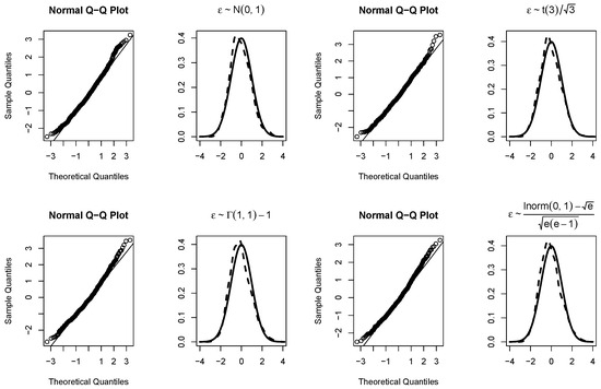
Figure 1. The null distributions and q-q plots of our proposed test when $g\left(u\right)=2u$.

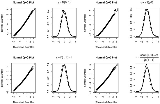
Figure 2. The null distributions and the q-q plots of our proposed test when $g\left(u\right)=2+sin\left(2\pi u\right)$.

For different $n,p$, Figure 3 and Figure 4, respectively, show the empirical power functions of the proposed test statistics. These figures are presented for four different error distribution functions. The function $g(·)$ is linear in Figure 3 and trigonometric in Figure 4. When $(n,p)=(200,201),(100,201),(200,365)$, the empirical power functions of the proposed test are represented by solid lines, dashed lines, and dotted lines, respectively. From Figure 3 and Figure 4, it can be seen that the power increases rapidly as long as c increases slightly. The test’s power is positively related to the sample size n and inversely related to the magnitude of p. The proposed test is stable under different error distributions. These are consistent with the conclusions in Table 3 and Table 4.

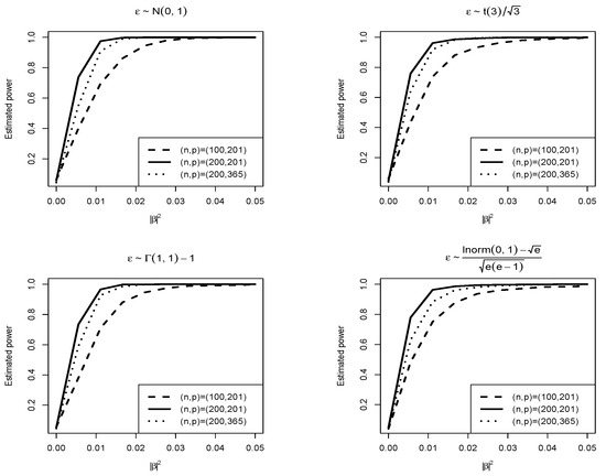
Figure 3. Empirical power functions of our proposed test when $g\left(u\right)=2u$.

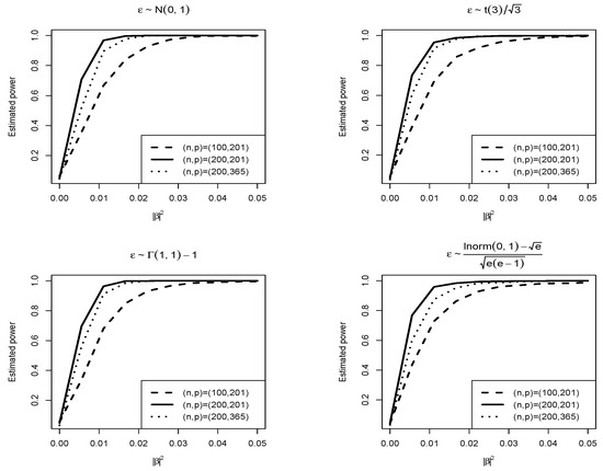
Figure 4. Empirical power functions of our proposed test when $g\left(u\right)=2+sin\left(2\pi u\right)$.

It is worth noting that, theoretically, a kernel function $K(·)$ is sufficient if it satisfies the conditions of symmetry and Lipschitz continuity. In practical applications, however, the choice of kernel function should be based on the characteristics and requirements of the data. For instance, the Epanechnikov kernel is more suitable for bounded data, while the Gaussian kernel is better suited for data with long tails. In this simulation study, according to the given data setting, the Epanechnikov kernel was chosen. To compare the effects of the two kernels, we replaced the Epanechnikov kernel used to generate Figure 4 with a Gaussian kernel to produce Figure 5. From Figure 4 and Figure 5, it can be observed that the impact of the two kernels on the test is relatively minor.

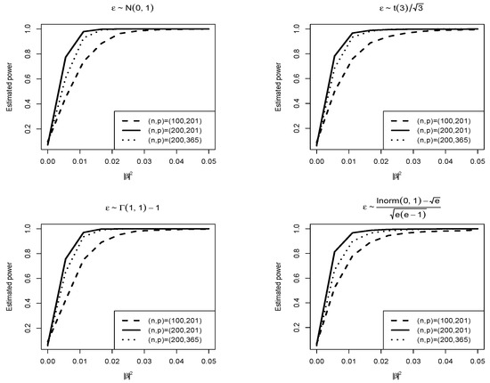
Figure 5. Empirical power functions of our proposed test with the Gaussian kernel when $g\left(u\right)=2+sin\left(2\pi u\right)$.

The numerical simulations show that our proposed test performs well for the data types. However, with larger sample sizes, the numerical simulations in this paper require considerable computational time, which is a limitation of the proposed test statistic. Additionally, its performance on the datasets that violate the assumptions (C1–C3) and (C7), such as when the real data are not in a Sobolev ellipsoid of order two, remains to be seen.

5. Application

This section applies the proposed test to the spectral data, which has been described and analyzed in the literature (see [25,26]). This dataset can be obtained on the following platforms: http://lib.stat.cmu.edu/datasets/tecator (accessed on 16 July 2024). Each meat sample is characterized by a 100-channel spectrum of absorbance, along with the moisture (water), fat, and protein contents. The absorbance is calculated as the negative logarithm base 10 of the transmittance, as measured by the spectrometer. The three contents, measured in percent, are determined by analytic chemistry. The dataset comprises 240 samples, partitioned into 5 subsets for the validation of models and extrapolation studies. In this section, we utilize a total of 215 samples, which include both training and test samples drawn from the 5 subsets. The spectral measurement data consist of curves, represented by $X_i(·)$, corresponding to absorbance values recorded at 100 equally spaced wavelengths from 850 nm to 1050 nm. Let $Y_i$ represent the fat content as the response variable, $Z_i$ represent the protein content, and $U_i$ represent the moisture content. Similar to [27], the following two models will be used to assume the relationship between them:

$$Y_i={\int }_{850}^{1050}\alpha \left(t\right)X_i\left(t\right)dt+g\left(Z_i\right)+{\epsilon }_i,$$

(10)

$$Y_i={\int }_{850}^{1050}\alpha \left(t\right)X_i\left(t\right)dt+g\left(U_i\right)+{\epsilon }_i.$$

(11)

The present investigation primarily focuses on the test in models (10) and (11): $\alpha \left(t\right)=0$. The number of basis functions used for fitting function curves p is selected as 129. Figure 6 shows the estimation of slope function $\alpha \left(t\right)$ in models (10) and (11).

Figure 6. (a) The estimator of the slope function in model (10); (b) the estimator of the slope function in model (11).

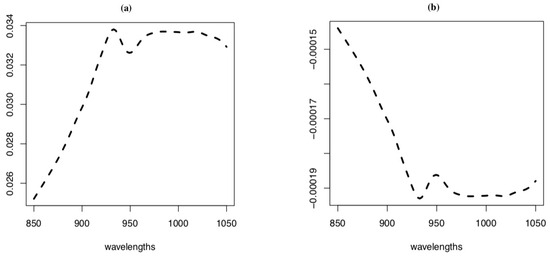
The calculation results are as follows: (i) For model (10), the value of the statistic is $T_{np}=31.186$; p-value is 0. (ii) For model (11), the value of the statistic is $T_{np}=-0.867$; p-values are 0.386. From this, we can see that the model test (10) is significant, while the model test (11) is not significant. This result can also be reflected in Figure 6. It is obvious that the estimated value of $\alpha \left(t\right)$ on the right side of Figure 6 is much smaller than that on the left side.

6. Conclusions

To test (2), this paper first provides a pseudo-estimate of the non-parametric function $g\left(u\right)$ using kernel methods with a fixed coefficient function $\beta \left(t\right)$. The pseudo-estimate is then substituted into the model, converting the original model into a linear one. This allows for the construction of the second-order U-test statistic employed in this paper, utilizing the corresponding testing methods from functional linear models. The proposed test does not require estimating the covariance operator of the predictor function. It follows a normal distribution asymptotically under both a null hypothesis and a local alternative. Moreover, numerical simulations show that our proposed test performs better than the test constructed in [18] when functional data cannot be approximated by a few principal components. Finally, the real data are applied to our proposed test to verify its feasibility.

Additionally, the proposed test is adaptable to cases where the response variable is functional, which is a focus for our upcoming research. In the real world, the proposed test requires real data to meet some technical conditions (C1–C3, C7). When data fail to satisfy these conditions, the viability of the test presented in this paper requires further investigation. Therefore, future work may focus on broadening the test’s applicability. The calculation of the statistics in numerical simulations requires optimization for efficiency.

References

- Crainiceanu, C.M.; Staicu, A.M.; Di, C.Z. Generalized multilevel functional regression. J. Am. Stat. Assoc. 2009, 104, 1550–1561. [Google Scholar] [CrossRef] [PubMed]
- Wang, J.; Zhou, F.; Li, C.; Yin, N.; Liu, H.; Zhuang, B.; Huang, Q.; Wen, Y. Gene Association Analysis of Quantitative Trait Based on Functional Linear Regression Model with Local Sparse Estimator. Genes 2023, 14, 834. [Google Scholar] [CrossRef] [PubMed]
- Kokoszka, P.; Miao, H.; Zhang, X. Functional dynamic factor model for intraday price curves. J. Financ. Econom. 2014, 13, 456–477. [Google Scholar] [CrossRef]
- Rigueira, X.; Araújo, M.; Martínez, J.; García-Nieto, P.J.; Ocarranza, I. Functional Data Analysis for the Detection of Outliers and Study of the Effects of the COVID-19 Pandemic on Air Quality: A Case Study in Gijón, Spain. Mathematics 2022, 10, 2374. [Google Scholar] [CrossRef]
- Yao, F.; Müller, H.G. Functional quadratic regression. Biometrika 2010, 97, 49–64. [Google Scholar] [CrossRef]
- Lian, H. Functional partial linear model. J. Nonparametr. Stat. 2011, 23, 115–128. [Google Scholar] [CrossRef]
- Zhou, J.; Chen, M. Spline estimators for semi-functional linear model. Stat. Probab. Lett. 2012, 82, 505–513. [Google Scholar] [CrossRef]
- Tang, Q. Estimation for semi-functional linear regression. Statistics 2015, 49, 1262–1278. [Google Scholar]
- Zhang, Y.; Wu, Y. Robust hypothesis testing in functional linear models. J. Stat. Comput. Simul. 2023, 93, 2563–2581. [Google Scholar] [CrossRef]
- Kokoszka, P.; Maslova, I.; Sojka, J.; Zhu, L. Testing for lack of dependence in the functional linear model. Can. J. Stat. 2008, 36, 207–222. [Google Scholar] [CrossRef]
- James, G.M.; Wang, J.; Zhu, J. Functional linear regression that’s interpretable. Ann. Stat. 2009, 37, 2083–2108. [Google Scholar] [CrossRef]
- Shin, H. Partial functional linear regression. J. Stat. Plan. Inference 2009, 139, 3405–3418. [Google Scholar] [CrossRef]
- Yu, P.; Zhang, Z.; Du, J. A test of linearity in partial functional linear regression. Metrika 2016, 79, 953–969. [Google Scholar] [CrossRef]
- Hu, H.; Zhang, R.; Yu, Z.; Lian, H.; Liu, Y. Estimation and testing for partially functional linear errors-in-variables models. J. Multivar. Anal. 2019, 170, 296–314. [Google Scholar]
- Smaga, Ł. General linear hypothesis testing in functional response model. Commun. Stat.-Theory Methods 2019, 50, 5068–5083. [Google Scholar]
- Zhu, H.; Zhang, R.; Li, H. Estimation on semi-functional linear errors-in-variables models. Commun. Stat.-Theory Methods 2019, 48, 4380–4393. [Google Scholar] [CrossRef]
- Zhou, J.; Peng, Q. Estimation for functional partial linear models with missing responses. Stat. Probab. Lett. 2020, 156, 108598. [Google Scholar] [CrossRef]
- Zhao, F.; Zhang, B. Testing linearity in functional partially linear models. Acta Math. Appl. Sin. Engl. Ser. 2024, 40, 875–886. [Google Scholar] [CrossRef]
- Hu, W.; Lin, N.; Zhang, B. Nonparametric testing of lack of dependence in functional linear models. PLoS ONE 2020, 15, e0234094. [Google Scholar] [CrossRef]
- Zhao, F.; Lin, N.; Hu, W.; Zhang, B. A faster U-statistic for testing independence in the functional linear models. J. Stat. Plan. Inference 2022, 217, 188–203. [Google Scholar] [CrossRef]
- Zhao, F.; Lin, N.; Zhang, B. A new test for high-dimensional regression coefficients in partially linear models. Can. J. Stat. 2023, 51, 5–18. [Google Scholar] [CrossRef]
- Cui, H.; Guo, W.; Zhong, W. Test for high-dimensional regression coefficients using refitted cross-validation variance estimation. Ann. Stat. 2018, 46, 958–988. [Google Scholar] [CrossRef]
- Zhong, P.; Chen, S. Tests for high-dimensional regression coefficients with factorial designs. J. Am. Stat. Assoc. 2011, 106, 260–274. [Google Scholar] [CrossRef]
- Chen, S.; Zhang, L.; Zhong, P. Tests for high-dimensional covariance matrices. J. Am. Stat. Assoc. 2010, 105, 810–819. [Google Scholar] [CrossRef]
- Ferraty, F.; Vieu, P. Nonparametric Functional Data Analysis: Theory and Practice; Springer: New York, NY, USA, 2006. [Google Scholar]
- Shang, H.L. Bayesian bandwidth estimation for a semi-functional partial linear regression model with unknown error density. Comput. Stat. 2014, 29, 829–848. [Google Scholar] [CrossRef]
- Yu, P.; Zhang, Z.; Du, J. Estimation in functional partial linear composite quantile regression model. Chin. J. Appl. Probab. Stat. 2017, 33, 170–190. [Google Scholar]
Disclaimer/Publisher’s Note: The statements, opinions and data contained in all publications are solely those of the individual author(s) and contributor(s) and not of MDPI and/or the editor(s). MDPI and/or the editor(s) disclaim responsibility for any injury to people or property resulting from any ideas, methods, instructions or products referred to in the content. |
© 2024 by the authors. Licensee MDPI, Basel, Switzerland. This article is an open access article distributed under the terms and conditions of the Creative Commons Attribution (CC BY) license (https://creativecommons.org/licenses/by/4.0/).